Scientific Investigations Report 2005–5215
U.S. GEOLOGICAL SURVEY
Scientific Investigations Report 2005–5215
Four transects were modeled to estimate seepage along the 3 river-mile reach of the Boise River (fig. 1). Each transect was represented by a two-dimensional VS2DI model. Due to data input limitations with VS2DI, five similar versions of the model were created for each transect, one for each month of the modeling period: April through August 2003. The ending conditions for the first model were copied into the following month’s model as initial conditions. The transfer of a model’s ending conditions to the following model’s initial conditions continued for the remaining model periods (modeling procedure is explained in detail under specific sections below).
Three categories of field data were collected for input into the modeling software to estimate ground- and stream-water seepage: (1) hydraulic conductivity of the subsurface sediments via slug tests, (2) monthly ground-water head and stream stage values, and (3) temperature measured at various depths and locations throughout the transect. These data were measured in various piezometers installed at each of the four transects.
As many as seven piezometers were installed at each of the four transects along the lower Boise River near Parma. One piezometer was installed in the center of the stream, one near each bank in the stream, one on each bank, and another installed a short distance from each bank of the stream (fig. 2). The piezometers were installed to a depth of 5.5 ft below the deepest part of the stream within each transect, and they were then surveyed to verify installation to the correct depth. Piezometers range in length from 8 to 16 ft, with buried lengths from 6 to 15 ft. The near bank and bank piezometers labeled B, C, E, and F in figure 2 were constructed of 1.25 inch diameter steel pipe with the bottom of the pipe pinched off to form a drive point. Above the drive point, the steel pipe was punched with holes on four opposite sides along a 6-inch length to allow water flow in and out of the piezometer. The other three piezometers labeled A, D, and G in figure 2 were created similarly, but from 0.75-inch diameter steel pipe. Each piezometer was developed after installation by pumping several bore volumes of water out of the piezometer.
It was possible to install all seven piezometers only at transect two; however, piezometer D in transect 2 was destroyed by high water flows early in the study period. Several attempts were made to install piezometer G at transect 1, but these attempts failed because of pipe breakage from a possible old roadbed in the subsurface. Piezometer D in transect 1 was destroyed in August. The river at transect 3 was too deep to install a center stream piezometer (D), and lack of access at transect 4 prevented the installation of piezometer G in that transect. Data loss because of the missing piezometers was limited to water-level measurements; compensations were made in the seepage modeling.
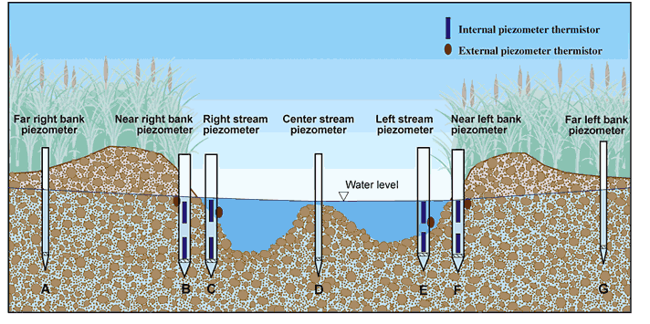
Figure 2. Schematic of piezometer installation, viewing the stream cross-section upstream.
Slug tests were conducted in the near-bank piezometers (piezometers B, C, E, and F) to estimate saturated hydraulic conductivity of the near-surface fluvial sediments. The slug test estimate of saturated hydraulic conductivity actually represents a small volumetric area around the perforated section of the piezometer The same method was used to perform all of the slug tests. Water levels for each slug test were measured with an In-situ mini-troll pressure transducer placed just above the perforated section of the piezometer. The pressure transducer has a 30-lb/in2 (equivalent to a 69-foot change in water level) range with an accuracy of ±0.02 percent full scale. The water level in the piezometer was measured with a calibrated electric tape, and was then programmed into the mini-troll. During the slug test, water levels were measured by the mini-troll every 0.50 second and were downloaded to a computer for analysis following the slug test.
To simulate an instantaneous injection of water, a bucket of water was used to fill the piezometer. Average time to fill the piezometer with water was approximately 1–3 seconds. The computer software AQTESOLV (Duffield, 2000) was used to analyze the slug tests. AQTESOLV provides three different slug-test solutions for unconfined aquifers: the Hvorslev (1951), Bouwer-Rice (1976), and KGS (Hyder and others, 1994). All three tests were used to analyze the slug-test data. Manual adjustments were made after automatic curve fits by AQTESOLV. The KGS model is more appropriate for sediments with high hydraulic conductivities similar to those found in most of the study area. Multiple tests were conducted on each piezometer to narrow variability with the slug-test analysis. The slug-test results are listed in table 1, with the piezometer name denoted by the transect number and piezometer letter. For example, piezometer E of transect 3 is labeled T3E. Slug-test estimates of saturated hydraulic conductivity ranged from less than 1 to 360 ft/d.
[Method of analyses: Bouwer-Rice (1976); Hvorslev (1951); KGS, Hyder and others (1994). Abbreviations: ft/d, foot per day]
| Piezometer | Test No. |
Saturated hydraulic conductivity (ft/d) |
Method of analysis |
|---|---|---|---|
| T1B | 1 | 121 | Bouwer-Rice |
| 2 | 68 | Bouwer-Rice | |
| 3 | 70 | Bouwer-Rice | |
| 1 | 124 | Hvorslev | |
| 2 | 77 | Hvorslev | |
| 3 | 79 | Hvorslev | |
| 1 | 63 | KGS | |
| 2 | 70 | KGS | |
| 3 | 68 | KGS | |
| T1C | 1 | 70 | Bouwer-Rice |
| 2 | 66 | Bouwer-Rice | |
| 3 | 70 | Bouwer-Rice | |
| 1 | 80 | Hvorslev | |
| 2 | 76 | Hvorslev | |
| 3 | 81 | Hvorslev | |
| 1 | 72 | KGS | |
| 2 | 71 | KGS | |
| 3 | 81 | KGS | |
| T1E | 1 | 139 | Bouwer-Rice |
| 2 | 128 | Bouwer-Rice | |
| 3 | 134 | Bouwer-Rice | |
| 4 | 134 | Bouwer-Rice | |
| 5 | 130 | Bouwer-Rice | |
| 1 | 159 | Hvorslev | |
| 2 | 152 | Hvorslev | |
| 3 | 159 | Hvorslev | |
| 4 | 159 | Hvorslev | |
| 5 | 154 | Hvorslev | |
| 1 | 142 | KGS | |
| 2 | 130 | KGS | |
| 3 | 145 | KGS | |
| 4 | 142 | KGS | |
| 5 | 146 | KGS | |
| T1F | 1 | 4 | Bouwer-Rice |
| 2 | 1 | Bouwer-Rice | |
| 1 | 4 | Hvorslev | |
| 2 | 1 | Hvorslev | |
| 1 | 4 | KGS | |
| 2 | 2 | KGS | |
| T2B | 1 | 128 | Bouwer-Rice |
| 2 | 142 | Bouwer-Rice | |
| 3 | 148 | Bouwer-Rice | |
| 4 | 124 | Bouwer-Rice | |
| 1 | 146 | Hvorslev | |
| 2 | 171 | Hvorslev | |
| 3 | 169 | Hvorslev | |
| 4 | 150 | Hvorslev | |
| 1 | 117 | KGS | |
| 2 | 113 | KGS | |
| 3 | 114 | KGS | |
| 4 | 111 | KGS | |
| T2C | 1 | 95 | Bouwer-Rice |
| 2 | 97 | Bouwer-Rice | |
| 3 | 95 | Bouwer-Rice | |
| 4 | 93 | Bouwer-Rice | |
| 1 | 120 | Hvorslev | |
| 2 | 118 | Hvorslev | |
| 3 | 114 | Hvorslev | |
| 4 | 112 | Hvorslev | |
| 1 | 93 | KGS | |
| 2 | 93 | KGS | |
| 3 | 95 | KGS | |
| 4 | 95 | KGS | |
| T2E | 1 | 42 | Bouwer-Rice |
| 2 | 44 | Bouwer-Rice | |
| 3 | 46 | Bouwer-Rice | |
| 4 | 48 | Bouwer-Rice | |
| 1 | 50 | Hvorslev | |
| 2 | 53 | Hvorslev | |
| 3 | 54 | Hvorslev | |
| 4 | 55 | Hvorslev | |
| 1 | 45 | KGS | |
| 2 | 48 | KGS | |
| 3 | 48 | KGS | |
| 4 | 51 | KGS | |
| T2F | 1 | 293 | Bouwer-Rice |
| 2 | 295 | Bouwer-Rice | |
| 3 | 310 | Bouwer-Rice | |
| 4 | 285 | Bouwer-Rice | |
| 1 | 342 | Hvorslev | |
| 2 | 343 | Hvorslev | |
| 3 | 362 | Hvorslev | |
| 4 | 332 | Hvorslev | |
| 1 | 238 | KGS | |
| 2 | 237 | KGS | |
| 3 | 251 | KGS | |
| 4 | 228 | KGS |
| Piezometer | Test No. |
Saturated hydraulic conductivity (ft/d) |
Method of analysis |
|---|---|---|---|
| T3B | 1 | 61 | Bouwer-Rice |
| 2 | 66 | Bouwer-Rice | |
| 1 | 71 | Hvorslev | |
| 2 | 78 | Hvorslev | |
| 1 | 60 | KGS | |
| 2 | 66 | KGS | |
| T3C | 1 | 46 | Bouwer-Rice |
| 2 | 45 | Bouwer-Rice | |
| 3 | 44 | Bouwer-Rice | |
| 4 | 44 | Bouwer-Rice | |
| 1 | 54 | Hvorslev | |
| 2 | 52 | Hvorslev | |
| 3 | 52 | Hvorslev | |
| 4 | 51 | Hvorslev | |
| 1 | 48 | KGS | |
| 2 | 46 | KGS | |
| 3 | 47 | KGS | |
| 4 | 45 | KGS | |
| T3E | 1 | 185 | Bouwer-Rice |
| 2 | 197 | Bouwer-Rice | |
| 3 | 195 | Bouwer-Rice | |
| 4 | 193 | Bouwer-Rice | |
| 1 | 225 | Hvorslev | |
| 2 | 219 | Hvorslev | |
| 3 | 226 | Hvorslev | |
| 4 | 225 | Hvorslev | |
| 1 | 175 | KGS | |
| 2 | 151 | KGS | |
| 3 | 148 | KGS | |
| 4 | 159 | KGS | |
| T3F | 1 | 222 | Bouwer-Rice |
| 2 | 235 | Bouwer-Rice | |
| 3 | 231 | Bouwer-Rice | |
| 4 | 229 | Bouwer-Rice | |
| 1 | 248 | Hvorslev | |
| 2 | 275 | Hvorslev | |
| 3 | 259 | Hvorslev | |
| 4 | 257 | Hvorslev | |
| 1 | 164 | KGS | |
| 2 | 155 | KGS | |
| 3 | 146 | KGS | |
| 4 | 168 | KGS | |
| T4B | 1 | 8 | Bouwer-Rice |
| 2 | 3 | Bouwer-Rice | |
| 3 | 5 | Bouwer-Rice | |
| 1 | 10 | Hvorslev | |
| 2 | 3 | Hvorslev | |
| 3 | 5 | Hvorslev | |
| 1 | 9 | KGS | |
| 2 | 4 | KGS | |
| 3 | 4 | KGS | |
| T4C | 1 | 0 | Bouwer-Rice |
| 2 | 0 | Bouwer-Rice | |
| 1 | 1 | Hvorslev | |
| 2 | 0 | Hvorslev | |
| 1 | 1 | KGS | |
| 2 | 0 | KGS | |
| T4E | 1 | 167 | Bouwer-Rice |
| 2 | 179 | Bouwer-Rice | |
| 3 | 177 | Bouwer-Rice | |
| 4 | 172 | Bouwer-Rice | |
| 5 | 178 | Bouwer-Rice | |
| 1 | 192 | Hvorslev | |
| 2 | 207 | Hvorslev | |
| 3 | 204 | Hvorslev | |
| 4 | 198 | Hvorslev | |
| 5 | 206 | Hvorslev | |
| 1 | 149 | KGS | |
| 2 | 128 | KGS | |
| 3 | 158 | KGS | |
| 4 | 145 | KGS | |
| T4F | 1 | 46 | Bouwer-Rice |
| 2 | 54 | Bouwer-Rice | |
| 3 | 62 | Bouwer-Rice | |
| 4 | 64 | Bouwer-Rice | |
| 1 | 53 | Hvorslev | |
| 2 | 63 | Hvorslev | |
| 3 | 72 | Hvorslev | |
| 4 | 73 | Hvorslev | |
| 1 | 47 | KGS | |
| 2 | 53 | KGS | |
| 3 | 61 | KGS | |
| 4 | 63 | KGS |
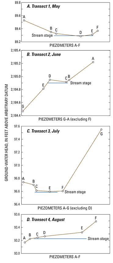
Monthly ground-water head measurements were conducted in all piezometers at each transect during the study period. Stream stage was measured at the same time as the ground-water head measurements by using a stilling well near a piezometer at each transect. Because each transect is located below a straight stretch of the river, stage mounding was not a concern. With the piezometers at each transect installed to the same depth, ground-water head measurements provide information on the horizontal hydraulic gradient. Comparisons between the ground-water head measurements and stream stage determines the relation between the two (gaining or losing stream) because the river and aquifer are in direct communication.
Elevations of the piezometers at transects 1, 3, and 4 were established using an arbitrary datum because only relative differences between the head and stage measurements were required. A known elevation datum was located near transect 2 so the head and stage values are based on actual elevations.
The ground water and river are hydraulically connected in this area throughout the season as indicated in figures 3A‑D. Head measurements in piezometers in the stream are very close to the stream stage, whereas head values in distant piezometers have a greater range than the stream stage. Transects 1, 3, and 4 were gaining streams, with varying vertical hydraulic gradients throughout the study period (figs. 3A, 3C, and 3D). Transect 2 was a losing stream during April, and then became a flow-through reach for the remainder of the study period. Transect 2 showed a hydraulic gradient from the east to the west, or from piezometer A to G (fig. 3C). Transect 4 also has an increasing horizontal gradient from the south to the north, or from piezometer F to A (fig. 3D).
The near-bank piezometers (B, C, E, and F) were each equipped with two continuous recording temperature thermistors installed at 1 and 5 ft from the bottom of the piezometers (fig. 2). One additional thermistor was either attached to the outside of the piezometer at the bottom of the stream for the instream piezometers, or was buried several inches below the bank surface for the piezometers installed on the banks. The external piezometer thermistor (StowAway TidbiT Temp Logger) and the internal piezometer thermistor (Optic StowAway Temp) are both made by the Onset Computer Corporation, Pocasset, Massachusetts. They measure temperature to within ± 0.4°C and record temperature within a range of -0.5° to 37°C. The thermistors were set to record temperature at hourly intervals from March 19, 2003 until retrieved on October 31, 2003. The temperature data for the upper interior thermistor in piezometer E of transect 1 could not be retrieved due to a malfunctioning thermistor. The temperature data were used primarily for the VS2DI modeling.
For more information about USGS activities in Idaho, visit the USGS Idaho Water Science Center home page .

![]() U.S. Department of the Interior |
U.S. Geological Survey
U.S. Department of the Interior |
U.S. Geological Survey
Persistent URL: https://pubs.water.usgs.gov/sir
Page Contact Information: Publications Team
Page Last Modified:
