Scientific Investigations Report 2008–5093
U.S. GEOLOGICAL SURVEY
Scientific Investigations Report 2008–5093
The primary objective of numerical modeling was to simulate the effects of changing river discharges and lake stages in the Dudley reach on velocities, bed shear stress, erosion and deposition, and sediment mobility. Successful models can be used to estimate water-surface elevations, flow depths, velocities, shear stresses, erosion, deposition, and sediment transport for flows of varying magnitudes and stages.
The HEC-6 computer model, version 4.2, (U.S. Army Corps of Engineers, 1993) was used to construct a sediment-transport model of the Coeur d’Alene River. Sediment-transport processes were not simulated in most previous modeling studies of this reach, and the streambed was assumed to be stable (fixed bed). However, in this study, sediment-transport processes were simulated because the model was developed to include a movable streambed. The modeled reach extended from Enaville on the NF to Springston, about 1.5 mi upstream of the Coeur d’Alene River inlet to the lake—an actual flow distance of 35.0 mi. The actual flow distance on the SF is 1.6 mi; therefore, the total model length is 36.6 mi.
HEC-6 is a computer program that analyzes 1D, gradually varied, steady flow in open channels with movable boundaries due to scour and deposition (U.S. Army Corps of Engineers, 1993). In areas where flow velocity is changing rapidly, the gradually varied flow assumption requires the use of closely-spaced cross sections. The HEC-6 model uses the standard step method (Chow, 1959) to determine changes in water-surface elevations from one cross section to the next by balancing total energy head at the sections. This 1D model assumes that energy is uniform in a cross section. This assumption is only valid at locations where flow is parallel to the main channel or where vertical velocities are not significant. The simulated channel does not account for debris because the model assumes unobstructed flow. Also HEC-6 cannot simulate flows through bridges or culverts because the program does not include equations to simulate these features.
HEC-6 allows for simultaneous erosion and deposition to occur depending on the competency of the stream to transport suspended sediment and bedload. However, HEC-6 does not allow bank erosion or lateral channel migration. This model can simulate the transport of sediment from upstream sources, transport of bed and suspended loads, and the effects of an armored surface layer on flow. The model can simulate transport of sediment sizes as large as 2,048 mm and includes 11 predefined sediment transport equations. The model also can simulate the transport of silt and clay. The model first calculates the water-surface elevation at each cross section using the standard step method. The potential sediment transport rate at each cross section, combined with the flow, determines the suspended sediment volume in each reach. If this volume exceeds the transport capacity of the reach, deposition occurs in the reach. If the volume is less than the transport capacity of the reach, scouring occurs. After each time step, the model updates the channel geometry in each section of the reach to account for the effects of scour and deposition. Finally, the flow value from the next time step is read and a new water-surface elevation is calculated using the updated channel geometries. This procedure is repeated until the model completes all specified time steps. The number of time steps is based on trial-and-error simulations to determine when changes in streambed elevations are minimal between one time step and the next. Sediment-transport calculations are performed by grain-size class, allowing the model to simulate hydraulic sorting and to control the rate of erosion and redeposition of sediment during the simulation period.
The HEC-6 model requires the user to select a sediment-transport equation. Eleven transport functions are available in the HEC-6 model. These equations were developed under different flow, hydraulic, and sediment conditions. Some of these equations are used for sandbed streams, gravelbed streams, or both; small streams, large streams, or both; and some are used to simulate bedload, suspended load, or both (total load). Stream-discharge equations based on stream-power concepts are more accurate than those based on other concepts, such as the shear-stress approach of Kalinske (1947) and Meyer-Peter and Müller (1948), the probabilistic approach of Einstein (1950), and the regression-equation approach of Rottner (1959), as described in Yang and Huang (2001) and Gomez and Church (1989). The Coeur d’Alene River study reach, required a sediment-discharge equation capable of computing the total load, consisting of sediment particles ranging in size from very-fine sands to cobbles. The Ackers and White (1973) equation fulfilled the transport equation requirement for the HEC-6 simulations. In a paper about accuracies of transport equations, Yang and Huang (2001) indicated the Ackers and White (1973) equation was accurate for a wide range of stream power and sediments sizes. Muskatirovic (2005) also showed that the Ackers and White (1973) equation fit measured data more closely than other equations for streams in the Salmon River Basin. This leads to the conclusion that use of a stream power type equation is a reasonable approach.
Model input consists of data describing cross sections, incoming sediment transport loads, distribution of streambed sediments, boundary conditions (discharge and stage), and time steps. The HEC-6 User’s Manual (U.S. Army Corps of Engineers, 1993) provides complete explanations of model input and shows examples of model inputs. An example of HEC-6 model input for calendar year 1999 is presented in appendix C.
The 234 cross sections used in the model included 62 that were surveyed in the field, 161 that were quantified using bathymetry and LIDAR data, and 11 that were interpolated from two adjacent surveyed sections. A series of maps in appendix A show the locations of cross sections. The field-surveyed cross sections are located in the braided reach, and cross-section data were collected using GPS and echo-sounder equipment, electronic total station, and (or) transit. Of the field-surveyed cross sections, four were used from the FourPt model (Woods and Beckwith, 1997) (cross sections 160.859, 161.705, 161.873, and 162.081) and three from the MIKE11 model (Borden and others, 2004) (cross sections 164.137, 167.004, and 167.676). The 161 cross sections developed from bathymetry and LIDAR data are located in the meander reach.
Seven bridges cross the river in the study reach—five roadway-highway and two bike trail. Three of the bridges (Highway 3 bridge near River Mile 150, Highway I-90 bridge, and old Highway I-90 bridge) have piers in the river. The ratio of bridge-pier area to flow area for these bridges was less than 5 percent; thus, the piers probably do not significantly constrict the river’s discharge through the bridge. HEC-6 does not allow for the simulation of bridges because the program does not include equations to simulate these features. Discharge measurements around these bridges during high flows would help determine if the configuration of these bridges and piers effect flow. However, cross sections at or near the bridges were used in the model.
Eleven interpolated cross sections (162.506, 162.599, 162.692, 162.948, 165.685, 165.719, 166.157, 166.255, 166.353, 166.543, and 166.636) were generated at various locations along the braided reach by interpolating data from two adjacent cross sections to minimize flow conveyance changes between the surveyed cross sections, thus, maintaining computational stability. For example, cross section 166.543 was interpolated from upstream cross section 166.729 and downstream cross section 166.451. Interpolation was computed by weighting the data from the two cross sections by the distance from the interpolated cross section. Interpolated cross section 166.543 was one-third of the distance from downstream section 166.451 and two-thirds of the distance from upstream section 166.729. This interpolation was done using a feature in the HEC-RAS model (Brunner, 2002a, 2002b; Warner and others, 2002). Interpolated cross sections improve model convergence and the solution used to determine the water surface.
The model used actual flow distances between cross sections, not the distance from subtracting river-mile designators for cross sections. Average difference in the study reach between actual flow and river-mile designator distances is about 35 ft. Using actual flow distances gives a better estimate of friction losses than using the more arbitrary river-mile designator distances. For example, the actual flow distance between cross sections 136.025 and 136.226 is 1,338.9 ft. Based on river-mile designators, the distance is 1,061.3 ft, a difference of 277.6 ft.
Flow in the study reach is subcritical. Therefore, the model requires discharge data at the upstream boundaries (cross section 168.713 on the NF and cross section 1.580 on the SF), and water-surface elevation at the downstream boundary (cross section 134.636). Discharge at the upstream boundary on the NF (cross section 168.713) was based on discharge data from the Enaville gaging stations (12413000). Discharge at the upstream boundary on the SF (cross section 1.580) was based on discharge data from the Pinehurst gaging station (12413470). Also discharge was added to cross section 166.729 near Kingston to account for additional discharge from intervening drainages and ground-water gains and losses between the NF and SF and the Cataldo gaging stations. Water-surface elevation at the downstream boundary (cross section 134.636) was based on adding stage data from the Harrison gaging station (12413860) and the NAVD 88 datum.
Calibration is the process of adjusting model parameters within reasonable limits to obtain the best fit of model simulation results to measured data. The process is to repeatedly adjust a parameter, run the model, and inspect the differences between model simulation results and measured data with the objective of minimizing the differences.
For this model, calibration consisted of comparing the difference between simulated and measured water-surface elevations at Rose Lake (12413810), Cataldo (12413500), Enaville (12413000), and Pinehurst (12413470) gaging stations (fig. 2). Four historical stage-discharge conditions in 1996 and 1997 were identified where discharge and water-surface elevation remained steady through the study reach at least for several days. During this period, high river discharges occurred and the Rose Lake gaging station was operational. Discharge on the main stem of the Coeur d’Alene River was based on daily mean discharge from the Cataldo gaging station. On the main stem just downstream of the confluence of the NF and SF at cross section 167.676, discharges from both river forks were added. Also on the main stem, discharge was added or subtracted to cross section 166.729 near Kingston to account for differences in discharge between the NF plus SF and the Cataldo gaging station. Discharges for the NF and SF were based on the Enaville and Pinehurst gaging stations, respectively, for the same period as the Cataldo gaging station. Water-surface elevations at gaging stations were calculated by adding the daily mean stage to the NAVD 88 datum and were calculated for the same period as discharges. In the model, Manning’s n values (roughness coefficient) were used as a calibration parameter. Model calibration was considered acceptable when the difference between simulated and measured water-surface elevations for each calibration condition was within ±0.15 ft.
Results from the water-surface elevation calibrations are shown in table 4. Differences in water-surface elevations ranged from -0.11 to 0.09 ft. Only Manning’s n values of the streambed were adjusted during this process because no field-determined n values were available. Adjustments were made equally to cross sections in each reach. Six reaches were defined, with the longest consisting of the entire meander reach (RM 134.6 to RM 159.8). The NF and SF also were defined as one reach. Figure 13 shows the final n values for the four reaches on the main stem. The n values for the NF ranged from 0.034 to 0.050, and SF ranged from 0.025 to 0.041. The n values in all six reaches decreased as discharges increased. No adjustments were made to the n values for the banks, which ranged from 0.029 in the meander reach to 0.045 in the NF and SF.
River discharge and stage data for calendar year 1999 also were simulated as a check on the reasonableness of sediment transport prior to attempting management simulations because no sediment-transport parameters were available to adjust in the HEC-6 model. Calendar year 1999 was selected because suspended-sediment samples were taken during that year and flow did not overtop banks and (or) levees. River discharges on the main stem were based on daily mean discharges at the Cataldo gaging station (12413500). River discharges for the NF and SF were based on the Enaville and Pinehurst gaging stations, respectively, for 1999. Water-surface elevations at the Harrison gaging station were calculated by adding the daily mean stage for 1999 to the NAVD 88 datum. The incoming total sediment discharges (QT) from the Enaville and Pinehurst gaging stations were estimated from QT curves shown in figure 12. A time step of 0.1 day was used requiring 3,650 iterations to complete the simulation for calendar year 1999.
Simulated HEC-6 sediment discharges for calendar year 1999 for sand transport (particle size equal to and greater than 0.00625 mm) are shown in figure 14. Measured and simulated sand transport were compared at the Rose Lake and Harrison gaging stations. Only sand transport was considered because sand particles are heavy enough to be deposited on the streambed, whereas clay and silt particles (considered the “wash load”) have low settling velocities and thus are transported in suspension with few of these size classes deposited on the streambed. Generally, simulated and measured sand discharges agreed with one another (fig. 14). Additional sediment samples at Rose Lake and Harrison and other areas in the study reach are needed—especially at higher river discharges—and would enhance existing datasets and allow the extension of sediment rating curves. Additional sampling also would help to improve model accuracy, especially during higher discharges when most transport occurs.
The calibrated model was verified as capable of simulating water-surface elevations and also was reasonable in simulating sand sediment discharge. Therefore, it can be used to test management alternatives such as dredging the streambed. The model can simulate changes in water-surface elevations, sediment transport, and streambed elevations (erosion and deposition) resulting from various alternatives. The HEC-6 model provides a dredging option to remove sediments from the streambed. Sediment transport, aggradation, and (or) degradation in the modeled reach are important factors, especially for determining substrate quantity.
For this study, four management alternatives were simulated. The configuration of the streambed in the model for all four management alternatives was altered in the Dudley reach to simulate dredging of the river channel. In management alternatives 3 and 4, the incoming total sediment discharge from the SF was decreased by one-half. Stage and discharge data for calendar year 2000 were used in alternatives 1 and 3 because river discharge probably did not overtop banks and (or) levees in the Dudley reach, and one large single peak (mean daily discharge of 26,100 ft3/s) was measured, which represents about a 4-year flood. The 4-year flood has a 25 percent chance of occurring in a given year. Stage and discharge data for calendar year 1997 were used in alternatives 2 and 4 because flows probably stayed within the confines of the channel in the Dudley reach, and several large peak flows were measured. The peak flows in 1997 were similar in magnitude to the single peak in 2000.
River discharges on the main stem were based on daily mean discharge at the Cataldo gaging station. Discharges on the NF and SF were based on the daily mean discharge at the Enaville and Pinehurst gaging stations, respectively, and water-surface elevations at Harrison gaging station were calculated by adding the daily mean stage to the NAVD 88 datum. On the main stem just downstream of the confluence of the NF and SF at cross section 167.676, discharges from both forks were added. Also on the main stem, daily mean discharge was added or subtracted near Kingston (cross section 166.729) to account for differences in daily mean discharge between the NF plus SF and the Cataldo gaging station. All simulations ran for one year using a time step of 0.1 day. An additional day was simulated in 2000 because it was a leap year.
For management alternative 1, river discharge and stage data from calendar year 2000 were used in the simulation. The incoming total sediment discharges from the NF and SF were determined from the total sediment discharge curves (fig. 12) for the respective river discharges. Before the simulation began, the configuration of the streambed in the model was altered at seven cross sections (156.135, 156.213, 156.286, 156.351, 156.399, 156.454, and 156.504) in the Dudley reach to simulate dredging of the river channel. These changes resulted in about 296,000 yd3 of streambed sediments being removed based on excavating about 20 ft of material over a 2,400 ft reach that averaged 175 ft in width. River discharge and model simulation results for sediment discharge for calendar year 2000 at cross section 156.504 (the upstream most cross section in the dredged reach) are shown in figure 15. Large amounts of sediment were transported on relatively few days in calendar year 2000 (fig. 15A). Model simulation results for April 15 showed that about 9,000 tons of sediment discharge were transported downstream of cross section 156.504. The peak flow of 26,100 ft3/s also occurred on this day and represents about a 4-year flood.
Also, model simulation results showed that about 6,530 yd3 of sediment were deposited in the dredged reach for 2000 (fig. 16), which represents 2.2 percent of the dredged sediments removed before the start of simulation. Thus for the long-term, it would take about 45 years to fill up the dredged reach to its original volume, assuming river conditions similar to 2000 occurred each year over that period. By the end of the simulation, the average increase in the streambed elevation in the Dudley reach was about 0.5 ft. The greatest increase in streambed elevation was about 1 ft at the upstream end of the dredged reach (fig. 16).
Because the 1D model does not simulate flow and sediment transport process on the floodplain, it is not clear how much erosion, deposition, and (or) sediment transport would occur in the channel due to flow that overtop banks. The flow that overtops banks along the Coeur d’Alene River probably is greater than the channel-forming discharge (bankfull flow) because of human influences, such as levees, along the river. Because no field data are available to determine bankfull flow along the Coeur d’Alene River, bankfull flow was estimated from flood frequency and was estimated to be the 2-year flood (18,900 ft3/s). Leopold (1994) indicated that bankfull flow usually ranges between the 1.5- and 2.5-year floods.
For alternative 2, the channel configuration was altered the same as in alternative 1 to simulate dredging. This alternative used river discharges and stages from calendar year 1997 because several large peak flows occurred during the year and flows and river discharge probably did not overtop banks and (or) levees in the Dudley reach. In addition, twice as many days of consecutive flow equaled and (or) exceeded bankfull flow (18,900 ft3/s) in 1997 than in 2000. The total flow volume in 1997 was 3 times greater than in 2000. The total flow volume for river discharges that equaled and (or) exceeded bankfull flow in 1997 was 2.3 times greater than in 2000. Nine days of flow exceeded bankfull flow in 1997 (fig. 15B). The highest daily mean flow in 1997 (25,300 ft3/s) (fig. 15B) was not as high as in 2000 (26,100 ft3/s) (fig. 15A). Model simulation results showed that the highest sediment discharge (about 12,000 ton/d on March 20) did not occur simultaneously with the highest peak flow of the year, but one day before the 4th highest peak flow. On the day of the highest peak flow (April 28), the simulated sediment discharge was ranked 7th out of 365 days. Model simulation results showed that about 12,300 yd3 of sediment were deposited in the dredged reach for the year (fig. 16), which was twice as much that was deposited in 2000. This value represents 4.2 percent of the total volume that was removed before the start of simulation in the dredged reach. Therefore, it would take about 24 years to fill up the dredged reach to its original volume assuming river conditions similar to 2000 occurred each year over that period. The thickness of deposition at the end of the simulation averaged about 1 ft in the dredged reach with the thickest of about 2.5 ft (fig. 16).
Management alternative 3 applied the same river discharge, stages, and incoming total sediment discharge, and streambed elevation as those in alternative 1, except that the incoming total sediment discharge from the SF was decreased by one-half. Model simulation results for this alternative were similar to those for alternative 1 (2000) in the Dudley reach, dredged, and downstream reaches. The decreased incoming total sediment discharge had no effect on the streambed in the Dudley, dredged, or downstream reaches. The distance of the river between the SF and Dudley reach probably is long enough for the sediment supply, transport capacity, and channel geometry to be balanced for the given discharge and stage conditions before reaching Dudley.
Alternative 4 was simulated using the same river discharges, stages, and incoming total sediment discharges, and streambed elevation as in alternative 2 (1997) except that the incoming total sediment discharge from the SF was decreased by one-half, as in alternative 3. Model simulation results for this alternative were similar to alternative 2 for the Dudley reach. Again, the decreased incoming total sediment discharge from the SF had no effect on model simulation results in the Dudley, dredged, and downstream reaches.
A computer model can be a useful tool for predicting water-surface and streambed elevations and sediment transport response to changes in the riverine system. However, the accuracy that a model can project water-surface and streambed elevations, and sediment transport is directly related to the accuracy and adequacy of the input data used to calibrate the model. The model limitations must be taken into account when using the model for projections.
The HEC-6 model contains many simplifying assumptions about the riverine system. Most important are the approximations of 1D flow, gradually varied flow, steady flow, movable streambed, and sediment transport. These simplifications might cause the model to calculate water-surface and streambed elevations and sediment transport with discharges greater than or less than experienced in actual study reach conditions. Overall, HEC-6 successfully calculated water-surface and streambed elevations and sediment transport in the Coeur d’Alene River. However, HEC-6 was not designed to account for uneven velocities in a cross section (especially in curved sections), uneven water-surface elevation in a cross section, or uneven erosion and deposition and sediment transport in a cross section. Also, HEC-6 does not provide the option to simulate infiltration losses and (or) gains in the channel.
The HEC-6 model cannot adequately simulate flow and sediment transport processes on the floodplain. Extreme events such as the 1996 flood that inundated the entire valley (channel and floodplains) cannot be simulated with this model and the effects are unknown. Also, the life expectancy of dredging from extreme events or bank overtopping flows is unknown. Only flows that stayed within the confines of the channel can be simulated with the HEC-6 model.
How velocity and sediment transport are distributed throughout the study reach evokes many questions that a 1D model like HEC-6 cannot answer. Applying multi-dimensional models that would simulate river discharge and sediment transport more precisely could refine velocity, bed shear stress, and sediment transport of the Coeur d’Alene River.
HEC-6 can simulate the transport of sediment sizes of 0.0625 mm (0.0025 in.) (very fine sand) and greater. The model can account for silt and clay particles less than 0.0325 mm (0.0013 in). However, shear threshold rates for clay and silt deposition and erosion were not available for the lower Coeur d’Alene River. These rates are site-dependent and may vary by orders of magnitude from one site to another; therefore, the results obtained from the model may not be reliable. Field measurements in the study reach are needed to determine actual shear threshold rates.
The particle size distribution of the streambed was limited to a few samples. Many more samples are needed throughout the study reach to characterize the streambed adequately. For the gravelbed reach, samples are needed of the armored layer and underneath the armor layer using specialized approaches for collecting samples with armored-surface layers as described in Berenbrock and Bennett (2005).
Suspended-sediment and bedload data were used to determine total sediment discharge at selected sites in the model. Since Clark and Woods’ (2001) study, no bedload samples have been collected, and their bedload curves were used without modification. The bedload curve for Rose Lake gaging station was based only on three samples (Clark and Woods, 2001, fig. 17), and at the Harrison gaging station, no bedload sediments have been collected by the sampler even at a discharge of 25,500 ft3/s. Thus, an assumption of zero bedload was made at the Harrison gaging station, which is unrealistic especially during higher discharges. Additional sediment samples at Rose Lake and Harrison gaging stations and at other areas in the study reach are needed and would enhance the existing dataset and allow for the extension of sediment rating curves. Additional sampling would help improve model accuracy especially during higher discharges when most transport occurs.
Two-dimensional (2D) models are able to simulate uneven water-surface elevations, varying velocities, and flows in more than one direction in a cross section. These models can also simulate the flow curvature in bends or eddies, whereas, flow curvature is lost in 1D models. Two-dimensional models also can provide better-defined velocities and hydraulic and bed shear stresses than 1D models. Therefore, the FASTMECH model, a 2D model, was used to simulate flow and hydraulic conditions for the Coeur d’Alene River in and around Dudley, Idaho.
FASTMECH is a computer program that analyzes 2D steady flow in channels and floodplains with a fixed bed. FASTMECH is a steady-state model using a structured curvilinear grid, based on the 2D, vertically averaged, shallow water equations (McDonald and others, 2001; Nelson and others, 2003; Simões and McDonald, 2004; and McDonald and others, 2006). The model also calculates the vertical distribution of the primary and secondary velocities about the vertically average velocity. These data help calculate the shear stress near the bed (τb). Vertical velocity distributions were estimated rather than computed from the shallow water equations; nevertheless, they add a partial dimensionality to the model. Thus, the FASTMECH model is designated as a two and one-half dimensional (2.5D) model.
The FASTMECH implementation encompassed the channel between RM 154 to RM 159 (fig. 17), a distance of 5.3 mi. The streambed in this model was assumed to be fixed and sediment-transport processes were not simulated. Nevertheless, bed and critical shear stress can be used for estimating sediment mobility, a surrogate of potential deposition and erosion. FASTMECH was recently applied to an 11-mi reach of the Kootenai River near Bonners Ferry with several sharp bends and split flow around an island (Barton and others, 2005). The model successfully simulated measured water-surface elevations and cross-stream velocities especially in bends. FASTMECH also has successfully simulated other rivers and floodplains (Conaway and Moran, 2004; Kenney, 2005; and Kinzel and others, 2005).
FASTMECH assumes flow is steady and incompressible. It also assumes flow is hydrostatic (neglecting vertical accelerations), and turbulence is treated adequately by relating Reynolds stresses to shear using an isotropic eddy viscosity (Nelson and others, 2003). Another FASTMECH assumption is that flow is unobstructed and free of debris in the channel and floodplain. The model uses only the International System (SI) of units. The SI system uses the metric system and meter of length, kilogram of mass, and second of time as its fundamental units.
FASTMECH was the first model incorporated into the Multi-Dimensional Surface Water Modeling System (MD_SWMS) (McDonald and others, 2001; and Simões and McDonald, 2004). MD_SWMS is a graphical user interface for pre- and post-processing application for computational models of surface-water hydraulics. MD_SWMS can be used to build, edit, and run models and view model inputs and results. The interface and additional information are accessible at http://wwwbrr.cr.usgs.gov/projects/SW_Math_mod/OpModels/MD_SWMS/index.htm.
The model grid used in FASTMECH is a curvilinear orthogonal coordinate system with a user-defined centerline. The grid centerline approximates the mean flow streamline in the modeling reach (Nelson and others, 2003) that was defined interactively in MD_SWMS. The computational grid used to model the Coeur d’Alene River was 8,452 m (27,730 ft or 5.3 mi) long with 3,371 nodes in the streamwise direction. The width was 350 m (1,148.3 ft) with 141 nodes in the cross-stream direction. This formed an approximately 2.5 × 2.5 m (8.2 × 8.2 ft) grid (fig. 17). Nodes are located at the corners of each grid, and 475,311 nodes form the computational grid.
A module in MD_SWMS was used to map bathymetry and LIDAR data to each node or coordinates of the model grid through a “nearest-neighbor” method. Bathymetry for each node was interpolated by a search bin that covered a predefined downstream length and cross-stream width. By choosing the length and width of the search bin judiciously, the user can tune the interpolation to treat situations where slopes in the cross-stream direction are steeper than slopes in the streamwise direction as frequently observed in alluvial rivers. Node interpolation includes all bathymetry and LIDAR data points in a search bin. If the search bin contains no data, the length and width of the search bin is doubled until at least one or more data points are found. Elevations of points in the search bin are weighted by distance from the node and averaged to obtain a value for each node of the grid. This approach works well where channel banks are nearly parallel to the grid as was the case for the modeled reach.
The FASTMECH model requires specific input parameters for each simulation. At the upstream boundary, the model requires river discharge. Discharge at the upstream boundary was based on discharge data from only the Cataldo gaging station (12413500). Flows from intervening drainages between the Cataldo gaging station and upstream model boundary are small compared to the river discharge in the main stem and were considered negligible in the model. Water-surface elevations at the downstream boundary were based on results from the HEC-6 model in a fixed-bed mode (see section on “HEC-6 Implementation” for more information on the HEC-6 model). Downstream water-surface elevations in the HEC-6 model were based on adding stage data from the Rose Lake gaging station (12413810) and the NAVD 88 datum. Boundary conditions for the calibration simulations are presented in table 5.
Calibration for a 2.5D model is similar to the calibration for a 1D model. A graphical and statistical model-calibration module contained in MD_SWMS allows for calibration with measured water-surface elevations and (or) velocities. To calibrate FASTECH, the drag coefficient was adjusted iteratively until simulated water-surface elevations matched measured water-surface elevations at selected sites. Physically, this process ensures the roughness used in the model accurately simulates head losses in the channel. Because measured values of water-surface elevations and velocities were not available, water-surface elevation values from FASTMECH were compared to HEC-6 at each cross section in the 5.3-mi modeled reach. No measured velocities were available for the calibration simulations, and thus, no additional adjustments were made to the drag coefficient because of velocity. For these calibrations, the model was run for 3,000 iterations, sufficient to achieve computational stability. Model calibration was considered acceptable when the difference between FASTMECH and HEC-6 water-surface elevations for each cross section was within the ±0.15 ft limit.
FASTMECH was calibrated to five historical discharge and water-surface elevation conditions (table 5). Selection of historical conditions for model calibration was based on two criteria. The first criterion was availability of water-surface elevation data at the Rose Lake gaging station (12413810). Second, because FASTMECH is a steady-state model, the historical discharge and water-surface elevation should be stable in the modeled reach for a minimum of 24 hours so river conditions approximate steady flow. Calibrated water-surface elevations at the downstream boundary ranged from about 2,130 ft to about 2,139.4 ft, and river discharges used in the calibration ranged from 10,500 to 28,900 ft3/s (table 5).
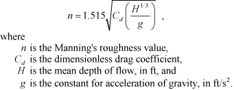
Each node was assigned an initial drag coefficient based on the roughness coefficient (Manning’s n) from the HEC-6 model. An equivalent Manning’s n value to the drag coefficient can be calculated using a depth scale from the following equation:
 (1)
(1)
The following example shows how using equation 1 estimated the initial drag coefficient. The fourth calibration simulation was used for this example, with a river discharge of 22,860 ft3/s and a daily mean water-surface elevation at the Rose Lake gaging station (12413810) of 2,139.43 ft (table 5). The HEC-6 model was simulated in a fixed-bed mode with these conditions. From the graph in figure 13, a Manning’s n coefficient for a river discharge of 22,860 ft3/s in the 2.5D modeled reach was interpolated to be 0.0224 for the streambed. From HEC-6 results, mean depth for the 2.5D modeled reach was 20.6 ft. Therefore, using equation 1, Cd was computed to be 0.0026. An initial Cd was computed for each calibration simulation and applied uniformly throughout the modeled reach.
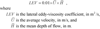
FASTMECH also incorporates a lateral eddy viscosity to represent lateral momentum exchange due to turbulence or other variability not generated at the bed (Nelson and others, 2003). The following equation can be used to compute the initial lateral eddy viscosity:
 (2)
(2)
Continuing with the previous example, the mean depth (![]() ) of flow is 20.6 ft. From HEC-6 results, average velocity for the modeled reach was 2.6 ft/s. The computed LEV value for this example is 0.16 m2/s. An initial LEV was computed for each calibration simulation and applied uniformly throughout the modeled reach.
) of flow is 20.6 ft. From HEC-6 results, average velocity for the modeled reach was 2.6 ft/s. The computed LEV value for this example is 0.16 m2/s. An initial LEV was computed for each calibration simulation and applied uniformly throughout the modeled reach.
Instead of measured water-surface elevation data, calibration simulations used water-surface elevation data derived from comparison of FASTMECH (simulated) and HEC-6 results. Comparisons between models were made at cross sections and at the center river node for the FASTMECH model. Differences in water-surface elevation between FASTMECH and HEC-6 were less than 0.15 ft, except at cross section 158.634 in simulation 5 (0.18 ft). Calibration results are shown in table 6 and figure 18. The mean absolute difference (MAD) error was small for all simulations. Water-surface elevations from FASTMECH and HEC-6 compared favorably (fig. 18). Along the middle part of the 2.5D reach from RM 156.5 to RM 158.5, water-surface elevations in FASTMECH were slightly less than elevations in HEC-6.Differences also were greater at lower discharges. Only drag coefficients (Cd) were adjusted during calibration.
Calibrated Cd values for each simulation are shown in table 6. The calibrated value in simulation 4 was slightly higher than the initial value and greater than all other simulations probably because the influence of backwater was greater due to the high lake stage. Water-surface elevation at the downstream boundary of the 2.5D model was about 2 ft higher in simulation 4 than in simulation 5, which had a greater river discharge (table 5). Table 6 also shows calibrated LEV values for each calibration simulation. The calibrated value in simulation 4 was lower than the initial value. This was true for all calibration simulations.
Results from the calibration simulations also included depth, velocity, bed shear stress, and sediment mobility. Each respective simulation used boundary conditions listed in table 5 with each respective simulation.
Simulated flow depths for river discharges of 10,500, 14,000, 17,300, 22,860, and 28,900 ft3/s are shown in figure 19. Usually depths increased as river discharge increased except for simulation 4 where the high lake levels in Coeur d’Alene Lake caused high water-surface elevations in the river due to backwater conditions. Water-surface elevation at the downstream boundary was about 2 ft higher in simulation 4 than in simulation 5 (table 5). However, river discharge in simulation 5 was about 6,000 ft3/s greater than in simulation 4. Simulated water-surface elevations throughout the modeled reach were higher in simulation 4 than in simulation 5. Therefore, flow depths were greater in simulation 4 than in simulation 5. The reach from RM 157.0 to RM 157.7 was the shallowest in all simulations (fig. 19), and the average simulated depth along the thalweg ranged from 16 ft in simulation 1 to 25.6 ft in simulation 4. The deepest point of the modeled reach occurred near RM 158.3 near a riverbed, and depths ranged from 43 ft in simulation 1 to 53 ft in simulation 4. In the dredged reach between cross sections 156.066 and 156.563, average depth along the thalweg ranged from 21 ft in simulation 1 to about 31 ft in simulation 4 (fig. 19).
Simulated flow velocities for river discharges of 10,500, 14,000, 17,300, 22,860, and 28,900 ft3/s are shown in figure 20. Simulated velocities increased as river discharges increased. Average simulated velocities along the thalweg ranged from about 3 ft/s in simulation 1 to 5.3 ft/s in simulation 5; maximum simulated velocities ranged from 3.9 ft/s in simulation 1 to about 7 ft/s in simulation 5. Velocities in simulation 4 were similar to velocities in simulation 3 because of the substantial backwater conditions in simulation 4 resulting from the high lake levels. In all simulations, the highest velocities occurred in the reach between RM 157.0 to RM 157.7 where flow depth is shallowest. In this reach, average velocity along the thalweg ranged from 3.5 ft/s in simulation 1 to about 6 ft/s in simulation 5. At the deepest point of the modeled reach (near RM 158.3), average simulated velocity ranged from 4 ft/s in simulation 1 to about 6 ft/s in simulation 5. In the dredged reach, from cross section 156.066 to section 156.563, average velocity along the thalweg was 2.75 ft/s in simulation 1 and 5 ft/s in simulation 5.
Velocity also can be described by magnitude and direction (vectors), whereas, velocity as described above was expressed only by magnitude (speed). Vectors usually are drawn as arrows pointing in the direction of flow with arrow color and (or) size depicting the speed of flow. Vectors of velocity are helpful in depicting the flow direction especially in reverse flows. Figure 21 shows velocity vectors of the dredged reach near Dudley. In the modeled reach, the vectors are nearly parallel except near banks and in and around river bends. The vectors also show that the highest velocities are near the center of the river probably aligned with the thalweg except in and around river bends. The maximum velocity at cross section 156.213 was 5.8 ft/s and average velocity was 3.5 ft/s, a decrease of 40 percent (fig. 21). On average, maximum velocities at cross sections shown in figure 21 (cross sections 156.135, 156.213, 156.286, 156.351, and 156.399) were about 60 percent greater than average velocity.
FASTMECH simulated several reverse flows (back-eddies). Several back-eddies occurred in a bend in the river near cross section 158.259 with a river discharge of 28,900 ft3/s (fig. 22). A large back-eddy near the left bank was about 120 ft wide and about 500 ft long and encompassed about one-third of the river width. Flow depth in the center of the eddy at cross section 158.259 was about 45 ft. Average flow depth throughout the eddy was about 22 ft. FASTMECH also simulated two other back-eddies on the right bank (fig. 22) . These back-eddies were much smaller in size and flow depths were much shallower. Other simulated back‑eddies in the modeled reach were much smaller than the large back-eddy at RM 158.3. No back-eddies were simulated by the model in the dredged reach (fig. 21). Back-eddies usually trap sediment and debris because of swirling or circular flows and slow velocities. If the velocities are slow enough, the sediments settle out.
In contrast to the multidimensional (FASTMECH) model, the 1D model (HEC-6) did not show or simulate eddies—even though a large eddy near cross section 158.259 occupies about one-third of the river (fig. 22). This deficiency illustrates why a 1D model is not appropriate for this reach. In 1D space, variables can have only one value. For example, a 1D hydraulic model can have only one value for each variable (velocity, water-surface elevation, shear stress, etc.) at a cross section. Rivers with eddies and other complex flow features cannot be expressed adequately in 1D space; therefore, multi-dimensional models are needed to simulate the river more precisely as shown in figure 22.
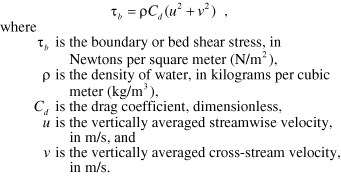
Shearing forces associated with river discharge, known as shear stress, determine the capability of a river to move material. Noncohesive sediment movement occurs when the boundary threshold is exceeded (Julien, 2002). The threshold is referred to as the critical shear stress. FASTMECH calculates boundary or bed shear stress as:
Simulated bed shear stress for river discharges of 10,500, 14,000, 17,300, 22,860, and 28,900 ft3/s are shown in figure 23. Simulated bed shear stress increased as river discharge increased. Average simulated bed shear stress ranged from 1.1 N/m2 in simulation 1 to 3.3 N/m2 in simulation 5. The maximum stress ranged from 3.3 N/m2 in simulation 1 to 10 N/m2 in simulation 5 with the highest stresses usually occurring in the river bend near RM 158. In the reach with the highest velocities and shallowest flow depths (RM 157.0 to RM 157.7), average stress along the thalweg ranged from 2.4 N/m2 in simulation 1 to 7.6 N/m2 in simulation 5. At the deepest point of the modeled reach (near RM 158.3), bed shear stress ranged from 3.2 N/m2 in simulation 1 to about 8 N/m2 in simulation 5. In the dredged reach, average stress along the thalweg ranged from 1.6 N/m2 in simulation 1 to 5.3 N/m2 in simulation 5, an increase greater than 200 percent.
The model-simulated bed shear stress also was used to assess sediment mobility over the five calibration simulations. River discharges for these simulations ranged from 10,500 to 28,900 ft3/s. Sediment mobility for a given particle size occurs when the boundary or bed shear stress (τb) exceeds the critical shear stress (τc), in other words τb > τc. This determines only whether a given particle size is potentially mobile. Sediment mobility provides an indication whether sediment movement (transport) occurs. However, bed erosion and deposition also depends on sediment supply. Sediment mobility is computed from flow depth and bed shear stress.
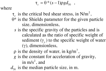
The following equation was used to determine critical shear stress for particle motion:
The Shields diagram provided the Shields parameter θ* for each particle size. Table 7 shows critical shear stresses and Shields parameter for the particle-size classifications of table 3. For example, critical shear stress for medium sand ranged from 0.194 to 0.27 N/m2.
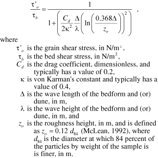
In sandbed channels where bedforms are present, such as the meander reach of the Coeur d’Alene River, total bed shear stress can be comprised of many components (McLean, 1992). Thus, for determining only the shear that is acting on the particles or grain, partitioning bed shear stress (τb) is necessary. Grain shear stress is the resistance due to sediment grains on the streambed and is responsible for the movement of sediment. The following equation was used to determine grain shear stress from total shear stress (Smith and McLean, 1977; and Nelson and others, 1993; Bennett, 1995, equation 9):
This analysis determines whether or not a given grain size is mobile, but does not calculate potential for erosion or deposition, which is determined by the divergence or convergence in the sediment transport rate, and is not addressed in this analysis.
Grain shear stress is determined in equation 5 by using dune height and length for a related river discharge. Because dune heights and lengths were not measured during the study, bathymetric data were used to determine if dunes existed in the 2D modeled reach. The only well-formed and continuous bedforms in the modeled reach were located near the downstream end of the modeled reach between RM 154 to RM 154.5. These dunes extended longitudinally and transversely (across) in the channel. Dune heights and lengths in this reach averaged 1.1 and 63 ft, respectively. Dunes of partial extent (ill-formed) also occurred in other areas of the model reach. Bedform geometry is dependent on the flow and sediment characteristics and sediment transport rate, and measurements of bedform geometry at different river discharges would help improve the accuracy of grain shear stress and sediment mobility potential.
Therefore, the average height and length of dunes from the bathymetry data near the downstream end of the modeled reach were used to determined grain shear stress and sediment mobility in the Dudley reach. Bed shear stress in the Dudley reach averaged 5.7 N/ m2 in simulation 5 (river discharge of 28,900 ft3/s). From equation 5, grain shear stress is calculated to be 3.5 N/m2 which corresponds to the largest particle size of 5.1 mm that can be mobilized. Because of the uncertainty in dune characteristics, grain shear stress was calculated for a range of dune heights and lengths—0.5 times (decreasing), 1.0 times, and 1.5 times (increasing). If the dune height was not 1.1 ft, but was 1.65 ft (1.5 times) (1.1 ft × 1.5 = 1.65 ft), grain shear stress would be 2.8 N/m2 and the largest mobilized particle would correspond to 4.1 mm; similarly, if only dune length was increased 1.5 times to 94.5 ft (63 ft × 1.5 = 94.5 ft), grain shear stress would be 4.0 N/m2 and largest mobilized particle would correspond to 5.7 mm. Because of the uncertainty in dune characteristics, grain shear stress was calculated for a range of dune heights and lengths—0.5 times (decreasing), 1.0 times, and 1.5 times (increasing). Table 8 shows grain shear stress, corresponding largest mobilized particle, and associated particle classification name for 0.5, 1.0, and 1.5 times dune height and (or) dune length for simulation 5 (river discharge, 28,900 ft3/s) based on an average bed shear stress of 5.7 N/m2 in the Dudley reach. Changes in grain shear stress were less than 3 times from one to another (table 8). If no bedforms existed in the Dudley reach, grain shear stress would be equivalent to the bed shear stress (5.7 N/m2) and the largest mobilized particle would correspond to 8 mm. Appendix D provides grain shear stress, largest mobilized particle, and particle classification for simulations 1 through 5. In simulations 1 through 5, areas of greater sediment mobility occurred near the thalweg where bed shear stresses (fig. 23) were greater; areas of lower sediment mobility occurred near the banks and back-eddies where bed shear stress were lower.
Several factors constrain the ability of the FASTMECH model to simulate water-surface elevations, velocities, bed shear stresses, and sediment mobility: (1) accuracy and detail of channel and bank geometry, (2) characterization of water-surface elevations and velocities, (3) characterization of bedform geometry, (4) potential errors incurred by applying a steady-state model to unsteady flow conditions, and (5) the 2D flow approximations.
FASTMECH was calibrated to the results from a 1D model, which limits the accuracy potential of the 2.5D model to that of a 1D model. The existing model calibration and any future model calibrations would benefit from the acquisition of actual water-surface elevations and velocities throughout the modeled reach for several river discharges to improve the accuracy of the model simulation results. Velocity conditions at the upstream model boundary profoundly affect flow for roughly the upper 0.5 mi of the model. Additional discharge measurements at several river discharges could help to determine the velocity distribution across the upstream boundary. Measurements of the bedform for a range of river discharges are needed to enhance estimates of grain shear stress and sediment mobility potential. Collection of particle-size distribution data along the streambed and banks also could enhance future model calibrations. This information would help to improve the accuracy of the modeled results especially for bed shear stress and sediment mobility potential, and thereby using the full potential of the 2.5D model.
A calibrated, transient, hydrodynamic model could provide a more thorough understanding of velocities, bed shear stresses, and channel evolution. Steady-state models, such as the one presented here, are unable to evaluate the effects of changing flow and lake-level conditions on bed sediment mobility. To better understand channel evolution, a transient-state, 2D sediment transport model would be beneficial. Also, this model is limited to river discharges contained within the banks and those flood flows that overtop the banks and spread onto the floodplain would have to be addressed by a multi-dimensional floodplain model with sediment transport capability.

![]() U.S. Department of the Interior | U.S. Geological Survey
U.S. Department of the Interior | U.S. Geological Survey
URL: http://pubs.usgs.gov/sir/2008/5093
Page Contact Information: Publications Team
Page Last Modified: Thursday, 10-Jan-2013 18:49:16 EST