Scientific Investigations Report 2010–5008
MethodsData SourcesData used for the regression models were obtained from four primary sources. Continuous streamflow data were obtained from stream-gaging stations (table 1) operated by USGS or the Oregon Water Resources Department (OWRD). Continuous data for field parameters (specific conductance and turbidity) were obtained from monitors operated by USGS at each site (table 1) for the study period or longer, although the monitors were removed at some sites during high flow in winter. Water-quality data for sampled constituents such as TSS, nutrients, and E. coli bacteria were obtained from autosamplers deployed during the study period (appendix A)and from historical datasets maintained by USGS (2001–07) and Clean Water Services (2001–04). USGS data primarily were available for the Fanno Creek at Durham Road site and were collected for various purposes; most high-flow water-quality data available for the Fanno Creek site were from the USGS historical database. Analyses included nutrients, suspended sediment, trace and major elements, and dissolved pesticides; however, only suspended sediment and TP were used for this report. Microbiological sampling, including E. coli bacteria, generally was not done by USGS during this period. Clean Water Services collects water-quality samples at least monthly at each of the study sites, and sometimes weekly, as part of its ambient monitoring program; however, high-flow periods are not specifically targeted and typically are under-represented in the Clean Water Services database. Clean Water Services sample analyses routinely include TSS, nutrients, and E. coli bacteria, among others. For the Dairy Creek site, Clean Water Services ambient monitoring data are the only available historical data, and are primarily from monthly samples. In addition, the available explanatory data are limited at this site because the continuous monitor was not deployed during winter until 2004–05. Finally, under certain conditions, streamflow at Dairy Creek can be affected by backwater from the Tualatin River, a situation that might invalidate any correlations established for unhindered flow conditions. MonitorsContinuous water-quality monitors were operated according to standard USGS protocols (Wagner and others, 2006). All monitors were the same, a YSI Environmental model 6920 multiparameter sonde equipped with probes to measure water temperature, specific conductance, turbidity, pH, and dissolved oxygen. Turbidity probes were YSI model 6026 probes, with the data reported in Formazin Nephelometric Units, or FNU (Anderson, 2004). Deployed monitors were cleaned and calibrated regularly, typically at 2-week intervals, and corrections due to cleaning and calibration were recorded. Data from the monitors were loaded into the USGS database and corrected to account for the effects of biofouling and sensor calibration drift according to procedures outlined by Wagner and others (2006). Each monitor was deployed in a 6-in. diameter PVC pipe mounted vertically on a steel post midstream at a height of approximately 6 in. to 1 ft above the streambed, with a locking cap for protection. The PVC pipe was perforated generously at the bottom to allow free circulation of stream water around the probes. Data were collected hourly. Periodically, and at a range of streamflows, the cross-sectional variation of monitor parameters was examined by making instantaneous measurements in a transect with a calibrated multiparameter instrument, and comparing the results to those logged by the monitor. The observed cross-sectional variability never exceeded the allowed calibration tolerances of the instruments; therefore, it was not necessary to adjust the monitor data to account for observed cross-sectional variations. Values for field parameters used in the regressions (specific conductance and turbidity) were obtained from the USGS continuous monitors rather than the Clean Water Services database when possible, for two reasons. Primarily, for making predictions of water-quality constituents during unsampled periods, the monitor data (and stream gages) are the only available source of independent variables. Therefore, the data used for constructing regressions should be collected in the same manner and be as internally consistent as the data used for making predictions. Secondly, turbidity data are known to be highly dependent on the optical configuration of the probe and potentially even the instrument model used (Anderson, 2004); therefore, consistency in long-term data collection methods is a critical factor when using turbidity as a surrogate for other parameters. For these reasons, the USGS has used the same models of turbidity probes throughout the monitoring network in the Tualatin River basin since their installation. Clean Water Services field data are from similar instruments, but calibration techniques and data management (especially policies on shifting data according to calibration errors) are different from those used by USGS. Furthermore, the Clean Water Services laboratory uses a bench top meter to measure turbidity, which is likely to produce different results than the USGS monitors because of critical methodological differences (Anderson, 2004). Nonetheless, for some periods, particularly at the Dairy Creek site where the USGS monitor was removed each winter during 2002–04, data from the continuous monitors were unavailable and Clean Water Services data were occasionally used to calibrate the regression models. For purposes unrelated to this study, the monitoring site in Fanno Creek was moved in 2003 from Durham City Park (fig. 2, site 1a) about 0.25 mi upstream to Durham Road (fig. 2; site 1b). Monitor and autosampler data were from the Durham City Park site until January 10, 2003, and from the Durham Road site thereafter. The potential influence of moving this station on development and interpretation of the regression models is discussed in the “Relations Between Continuous Monitor Data and Selected Water-Quality Constituents” section. Streamflow was continuously recorded at some sites (see table 1), either by USGS (Rantz and others, 1982) or by OWRD, according to standard USGS methods. The Dairy Creek site at Highway 8, which is about 2 mi from its junction with the Tualatin River, is susceptible to backwater from the Tualatin River during high flows in winter. Oregon Water Resources Department (ORWD) considers the stage-discharge rating at this site to be unreliable at a stage greater than about 10 ft (D. Hedin, Oregon Water Resources Department, written commun., July 2008), although the rating may be reliable at stages as high as 15–16 ft when flows in the Tualatin River are not high. OWRD does not provide streamflow records for stages greater than 10 ft at this site. At the non-target sites Rock Creek and Beaverton Creek, which were ungaged, streamflow records at the monitor site were reconstructed by simple summation and routing of upstream, recorded discharges. Travel times from upstream sites were estimated by examining streamflow data at upstream sites combined with monitor data (especially turbidity and specific conductance) during storms to determine the timing of discharge peaks. The difference in timing of the peaks was used to linearly adjust upstream discharges to represent flow at the downstream sites. Attempting to simulate the discharge record during storms at the Beaverton and Rock Creek sites in this manner (that is, without a more extensive hydrologic modeling approach) exposed difficulties in the use of discharge as an independent variable for developing predictive regression models at ungaged sites, contributing to these sites’ consideration as non-target rather than target sites. AutosamplersAutosamplers were operated as temporary installations for the duration of each storm or sampling event. Autosamplers used were ISCO, Inc., Model 6712 portable samplers, equipped with level sensors. Samplers were placed in a secure, level position on the streambank adjacent to the continuous monitors. Where possible, the samplers were housed in portable, locking fiberglass enclosures. Each sampler included a peristaltic pump to draw water from the stream through 3/8-in. inner-diameter vinyl tubing. Together with a communications cable from the water-quality monitor, this tubing was anchored to concrete blocks along the streambed. The intake tubing was positioned following USGS guidelines as summarized by G.D. Glysson, U.S. Geological Survey, written commun., 2009, and shown in table 2, except for items 3–5, which could not be determined with available resources for the study sites. The mouth of the vinyl tubing was secured to the perforated section of the monitor casing, oriented along the direction of flow and pointing downstream, an orientation that has been shown to minimize adverse sampling effects for pumping samplers (Winterstein, 1986). Because of pumping constraints, efforts were made to minimize the length of tubing between the monitor and the autosampler, typically 12 to 25 ft, with resultant vertical heads between 2 and 10 ft. Complete elimination of dips in the tubing that might trap heavy sediment particles was not possible; however, an effort was made to minimize the dips in the tubing. Each autosampler was configured with a carousel holding twenty-four 1-L polyethylene bottles. Prior to each deployment, the vinyl tubing and polyethylene bottles were cleaned with hot tap water and phosphorus-free detergent and thoroughly rinsed with deionized water. Upon deployment, the middle of the carousel in the autosampler was loaded with ice. Once deployed, samplers were visited at least once daily to check on the operation of the monitor and the sampler, and to change sample bottles, batteries, or ice, as necessary. The water-quality monitor and a separate water-level sensor were interfaced with the autosampler’s programmable computer. The ISCO water-level sensor used a pressure gage to sense the back pressure on air bubbled slowly through a small diameter tubing, the mouth of which was anchored to a fixed position in the stream. The water-level sensors proved to be unreliable and ultimately were used only for qualitative purposes to verify the timing of the streamflow peak rather than as a trigger for sampling or for depth data that could be used for correlations. Therefore, the autosamplers were programmed to use only turbidity data from the continuous monitor and were interrogated at 5-minute intervals, to trigger the sampling. Turbidity was considered the most reliable indicator that the stream was responding to a storm; an increase in turbidity of 10–15 FNU typically was used as the threshold for beginning sampling. Once triggered, the samplers were programmed to collect samples hourly, with a maximum of 24 bottles, and to record the monitor data and the time when each sample was collected. Prior to collecting each sample, the autosampler purged the vinyl sample tubing with air to remove any residual water and sediment, then performed three complete stream-water rinses of the line between the stream-end of the tubing and the liquid detector at the peristaltic pump head. Upon successful sample collection, the numbered bottles were retrieved and transported on ice to the Clean Water Services water-quality laboratory. The position of each bottle in the carousel was recorded, and the sampling data (timing of sample collection, water level, and water‑quality data from the continuous monitor) were downloaded from the autosampler. Autosampler data from this study are reported in appendix A. Autosampler Quality AssuranceSeveral issues potentially affecting the quality of data from autosampler-collected samples were identified and investigated at the beginning of the study. These included possible cross-contamination of samples from the vinyl autosampler tubing, which could not be washed between individual samples, and the degree to which samples collected by the autosampler at a point in the stream were comparable to those collected by standard USGS depth- and width-integrating and ultra-clean sampling protocols (Horowitz and others, 1994; Edwards and Glysson, 1999; G.D. Glysson, U.S. Geological Survey, written commun., 2009) . Cross-contamination initially was assessed in the laboratory by manually directing the sampler to collect a sequence of samples (three replicates each) from vats containing the following materials:
The resuspended mixture of tap water and soil (step 2 above) could not be uniformly mixed; therefore, results were not expected to be precise for analyses affected by particulates in water, such as TP. The point of using the soil mixture was to evaluate the extent of carryover of particulates to the subsequent deionized water samples. Samples from this series of tests were analyzed for nutrients (whole and filtered water) and chloride (filtered). For the synthetic standard samples, these tests also functioned as an evaluation of accuracy and precision in the sampling‑analysis process. The results of this series of tests generally were good and indicated that carryover of contamination from sample to sample using autosamplers with appropriately cleaned and maintained equipment was minimal, and could not be distinguished from background laboratory contamination levels (table 3). A low level of contamination of blank water by soluble reactive phosphorus was detected in laboratory blank samples shown in table 3 (test 1, 0.009 mg/L as P) and in two of three initial blank tests through the autosamplers (test 4, 0.007 mg/L as P). Only one sample indicated a small carryover of suspended material, as measured by total Kjeldahl nitrogen (TKN), a low concentration (test 6, 0.055 mg/L as N) just above the detection limit, in the first blank deionized water replicate following the soil mixtures. Considering that environmental concentrations of nutrients in storm runoff in the study streams were expected to be approximately 5–10 times higher than any contamination level detected in these tests, it was determined that neither contamination nor carryover was a major problem from the autosampler configuration. For the most part, results from the synthetic standard samples were within expected ranges. However, TKN concentrations in the low- and high-level synthetic standard samples (tests 2 and 3) seemed to be biased low by about 25 to 50 percent and the TP concentration in the high-level synthetic standard (Test 3) was almost 20 percent lower than expected. The synthetic standard tests were not repeated for this study, but they are repeated monthly as part of an ongoing quality‑assurance program between the USGS and Clean Water Services. For 2002–03, TKN analysis of synthetic standard and spiked river water samples by Clean Water Services consistently had recoveries of 90–100 percent compared to expected values, indicating that the low recoveries for TKN shown in table 3 were anomalous. For TP, recoveries from the USGS-Clean Water Services Quality Assurance program during 2002–03 tended to be lower than for TKN, about 80–90 percent, but also were relatively consistent. For field deployments of autosamplers, the determination of cross-section coefficients (also known as a box coefficient) is used to evaluate how point concentrations derived from an autosampler compare to depth- and width-integrated samples from across the range of streamflow conditions at the site (G.D. Glysson, U.S. Geological Survey, written commun., 2009). The coefficients also can be used to make corrections to autosampler data, if necessary. The box coefficient is calculated as the Ci/Cp, where Ci is a concentration derived from depth- and width-integrated sampling techniques, and Cp is the concentration from a pumping sampler. If the cross-section coefficient is near 1 for a given hydrologic condition, then no adjustment in concentrations is advised. Box coefficients and carryover through autosampling were assessed at base flow in Fanno Creek through a comparison of replicate stream-water samples collected using the autosampler, with samples collected using depth- and width-integrating techniques according to USGS protocols (table 4). An additional comparison was completed at Dairy Creek during mid-winter storm sampling. Some minor variations were observed in the determinations of autosampler box coefficients, but these were within analytical uncertainty. For example, the calculated box coefficient for TSS at Fanno Creek is 0.75; however, upon closer examination this primarily may be a result of laboratory variability. The triplicate cross-sectional samples (taken as aliquots from a churn splitter from a single depth- and width-integrated sampling) had moderate variation in the reported laboratory TSS concentrations (standard deviation 2.5), resulting in a median total TSS of 3 mg/L, whereas the replicate autosampler values were identical at a similar concentration (4 mg/L). E. coli bacteria counts showed the largest variability and the lowest box coefficient; however, bacteria counts also are known for their variability using current techniques and the differences shown here are not of concern at the low levels observed. Similarly, results of autosampler and equal width increment samples at Dairy Creek during a storm sampling in November 2003 were within 8 percent for all constituents and are indistinguishable from analytical variability. Adjustment of autosampler data by the box coefficient is not warranted by data in table 4 or by comparison with laboratory analytical uncertainty. However, additional comparisons at higher discharge (and higher suspended sediment concentrations) still are warranted to verify these findings under varying conditions and at different sampling sites. To further evaluate carryover, the streambed was stirred to suspend sediments upstream of the autosampler intake, and samples were collected from within that plume and after the plume had passed or settled (approximately 15 minutes), as turbidity at the monitor returned to its baseline value. As expected, samples from the period when the streambed was being disturbed (sequence numbers 8–10, table 4) showed a high degree of variability, which is not a concern because the disturbance was essentially random. More importantly, after settling samples for all constituents (sequence numbers 11–13, table 4) were not much different from those prior to the disturbance of the streambed. Clean Water Services LaboratoryAutosampler-derived water samples were analyzed by Clean Water Services at their water-quality laboratory in Hillsboro, Oregon. Samples were delivered immediately after retrieval from the autosamplers and subsampled for the indicated constituents (table 5). The analyzed constituents consisted of nutrients, suspended solids, bacteria, and chloride, several of which are regulated by the TMDL (Oregon Department of Environmental Quality, 2001). E. coli bacteria were analyzed immediately upon sample delivery to the Clean Water Services laboratory. Analyses for total and dissolved nutrients and TSS were started within 1–3 days of sample delivery, well within allowable holding times. Analytical methods and reporting limits are indicated in table 5. Laboratory Quality AssuranceThe Clean Water Services water-quality laboratory has a rigorous internal quality-assurance program. The laboratory also participates in the USGS national Standard Reference Sample (SRS) program, a national interlaboratory comparison study (see http://bqs.usgs.gov/srs/). Results from many years of participation in the SRS program have shown that the Clean Water Services laboratory consistently produces results that are sufficiently accurate for the parameters in this and other studies (bacteria are not included in the SRS). During 2002–05, Clean Water Services laboratory results for TP samples across a broad range of nominal concentrations (0.085–1.35 mg/L) were biased low by about -2 to -8 percent in 13 of 17 samples, and biased high by about 0 to 5 percent in 4 samples. Likewise, results from the TKN samples were biased low by about -1.5 to -16 percent in 8 of 10 samples, and biased slightly high (as much as 2.5 percent) in the remainder. Furthermore, the Clean Water Services laboratory methods and protocols have been reviewed by the USGS Branch of Quality Systems and were determined to be suitable. The Clean Water Services laboratory also participates in an annual Tualatin River basin Interlaboratory Comparison Study, which includes all laboratories that routinely analyze water samples for government agencies in the Tualatin River basin. On the basis of standard samples from both the Oregon Water Science Center (ORWSC) and national programs, TP data from Clean Water Services used in this study most likely were biased slightly low, but generally were consistent. The data, therefore, were unadjusted and considered adequate for the purposes of the study. When data from USGS and Clean Water Services laboratories are used together, any potential differences are reflected in the statistical uncertainty for the individual correlations. Ultimately, TKN was not included in the regression analysis, and any potential bias therefore was not relevant to the results of the study. Field methods in use by Clean Water Services are similar to those used by USGS, including the collection of samples using depth- and width-integrating techniques and the use of churn splitters for subsampling; therefore, the respective laboratory methods are the most likely sources of any differences between the two datasets. Previous studies (Horowitz and others, 1994; Gray and others, 2000) have demonstrated that analysis of total suspended solids (TSS), the analytical technique used by Clean Water Services and many other agencies, is often biased low compared to the analysis for suspended sediment concentration (SSC), as practiced by USGS. The difference in results between the methods is primarily attributed to subsampling; specifically, the SSC method includes measurement of sediment in the entire sample, but the TSS method measures sediment amounts in a subsample removed from the original sample bottle. The subsampling process can underestimate sediment concentrations, especially if sand concentrations are high or flocculation occurs, because these particles settle quickly in a sample bottle, and obtaining a representative subsample is difficult (Gray and others, 2000). No data are available for direct comparison of SSC and TSS in the USGS and Clean Water Services databases, respectively. For this report, the TSS and SSC data were combined without adjustment, and the variability introduced by the two methods is therefore incorporated into the regression results. Data AggregationThe intent of this report is to use the available datasets for model development and calibration, and to compare the most promising model forms and their resulting coefficients, to determine the likelihood that suitable predictive models can be used to understand transport and loading of the indicated constituents (TSS, TP, E. coli bacteria) at the Fanno and Dairy Creek sites. The data were aggregated into data scenarios, to evaluate (1) model calibration using the autosampler-only dataset, and model validation using available Clean Water Services data; (2) model calibration with the autosampler data plus the available historical USGS data, and model validation with Clean Water Services data; and (3) a combined dataset using data from all sources for calibration, while retaining independent data for model validation. Details of these scenarios for Fanno Creek at Durham are shown in table 6 and figure 3. During the model construction process, if the input variables identified as contributing the most information remained similar regardless of the scenario used, and likewise if the regression coefficient values remained moderately consistent for a given predicted variable regardless of scenario, then it could be concluded that the models were relatively robust and could be used reliably until additional data are collected that can be used to refine those models. On the other hand, if the use of different datasets resulted in widely varying model forms and coefficients, or goodness‑of‑fit diagnostic statistics that differ greatly, then additional and targeted data most likely are needed prior to development of useful models. All independent variables (specific conductance and turbidity data plus streamflow or stage) were consistently taken from the same data sources for all scenarios and model runs. Data from continuous monitors came from USGS, and streamflow or stage data came from USGS for Fanno Creek and from OWRD for Dairy Creek at Highway 8. Duration curves are commonly used in hydrologic studies to document the range of conditions measured at a site during an indicated period, including the frequency and magnitude of certain conditions. These curves depict cumulative distributions of all measurements during the study period, and show the percentage of time during the study period that specific values for the constituent were equaled or exceeded. Although typically used for discharge records, duration curves have increasingly been constructed for water quality constituents for which high density data can be collected, including continuous monitoring data such as those collected in this study (Rasmussen and others, 2008). Duration curves (fig. 3) for selected continuous parameters used in the regressions provide information about the relative magnitude of the parameter values during sampling, compared to the full range measured at the site during the study period. For example, if a given turbidity associated with a particular sample was exceeded only 5 percent of the time during the study period, then that measurement represents a relatively high turbidity; however, if the turbidity of a sample was exceeded 50 percent of the time or more often, then that sample represents average or low-flow conditions, respectively. During the early phases of model development, it was determined that exclusive use of the autosampler-derived data (Scenario 1) to construct predictive statistical models was flawed because of correlation issues. The regression process assumes that input data points are truly independent; however, data collected over a single hydrograph are not completely independent of one another. For example, as streamflow increases during a storm, samples collected sequentially are more likely to be similar to each other than samples collected during different storms or under completely different sampling conditions. This serial correlation is a problem when using the Scenario 1 (autosampler-only) dataset for model building purposes. Methods to account for serial correlation are available, such as introducing a lag in the data to reduce the interdependence of individual samples (Helsel and Hirsch, 1992); however, these methods were not used in this study because it was recognized that, whether or not a lag was introduced to account for serial correlation, the Scenario 1 datasets would be insufficient for regression modeling because the range of stream conditions encompassed by the autosampler deployments was limited (fig. 3A). As an example, the peak discharge sampled by the autosamplers at Fanno Creek was about 134 ft3/s (table 6); although discharges during the study period were as much as 780 ft3/s (fig. 3) and historical high flows occasionally have been greater than 1,000 ft3/s. For the purposes of simplicity and to focus on the larger study objectives, serial correlation was therefore ignored in the analysis of Scenario 1 and 2; instead, the Scenario 3 dataset was created to avoid serial correlation (see below). When appropriate, the potential influence of serial correlation on model development based on Scenario 1 and Scenario 2 is discussed. In Scenario 2, Fanno Creek autosampler data are augmented with additional data collected by the USGS for water years 2001-07 (table 6 and fig. 3B); validation is done with Clean Water Services data as in Scenario 1. Scenario 2 provides an example of one relatively simple method to aggregate data when multiple sources are available. Serial correlation between autosampler-derived data remains an issue in Scenario 2, although the influence of serial correlation on the outcome is reduced by the additional data. USGS data were collected for various purposes, including routine monitoring (USGS National Water-Quality Assessment Program, http://water.usgs.gov/nawqa/) and other, more targeted studies (McCarthy, 2000; Anderson and Rounds, 2003), and are stored in the USGS National Water Information System (NWIS) database (http://nwis.waterdata.usgs.gov/or/nwis/qwdata). The USGS and Clean Water Services routine monitoring designs do not target specific flow conditions, and the resulting dataset is primarily composed of base-flow (non-storm) samples during all months; high-flow samples are present only when storm events coincided with scheduled sampling events. At least one USGS study (Anderson and Rounds, 2003) did focus on high-flow and runoff conditions, thus providing several samples at discharges greater than those sampled by the deployed autosamplers. Additionally, occasional USGS and Clean Water Services samples were collected prior to 2002 at higher discharges, but continuous monitors were not deployed at the time so the results could not be used for this study. Scenario 3 was created specifically to minimize the stated problems in the Scenario 1 and 2 datasets. To avoid the serial correlation bias, Scenario 3 used only the autosampler data collected during peak flow in each individual storm sampled (that is, one sample per storm); to minimize base-flow bias, a subset of the routine Clean Water Services ambient monitoring data was used with selected high-flow data from the USGS and Clean Water Services historical datasets. From the routine Clean Water Services data, only the first data point in each month was included, which reduced the number of base-flow samples but still represented seasonal patterns; sometimes these samples represented moderate storm runoff, although most samples were collected at relatively low flows. For high flow, any samples that were potentially representative of storm response were desired; thus, high flow was determined as any data point with an associated discharge greater than the 25th percentile value for that month, as defined from monthly flow‑duration statistics computed from the NWIS database for the period of record at Fanno Creek near Durham (USGS stream-gaging station 14206950), October 2000–September 2007. This strategy allowed Scenario 3 to capture summer and spring storm responses while minimizing samples corresponding to low flows. Because of the paucity of high-flow samples, most available samples were used for calibration; however, a few were retained for validation (fig. 3C). For Scenario 1, the highest discharges sampled for model calibration were exceeded about 10 percent of the time from water year 2001 to 2007 (fig. 3). The Scenario 1 validation dataset (in black) has three samples at slightly higher discharges (exceeded about 7–9 percent of the time). By far the bulk of the samples were at discharges exceeded about 10–70 percent of the time, during base-flow to moderate storm runoff. The addition of data from USGS in Scenario 2, and re-aggregation to use a broad range of the samples from Clean Water Services’ database in Scenario 3, added successively greater numbers of samples from higher discharges, or those exceeded less than 1 to about 10 percent of the time. However, even in Scenario 3 only a few of these higher flow samples were available, and some were needed for model validation, whereas in each scenario large numbers of samples were collected during relatively low-flow conditions, when the respective discharges were frequently exceeded. Any potential contamination detected during the autosampler quality-assurance tests (table 3) was well below most of the sample concentrations included in the aggregated datasets. For example, although soluble reactive phosphorus was detected in blank water at 0.007–0.009 mg/L, the minimum TP concentrations in Scenarios 1, 2, and 3 were 0.08 mg/L, and the medians ranged from 0.13 to 0.15 mg/L (table 6). Maximum ambient concentrations for model calibration were as much as 0.47 mg/L. Even if contamination at less than 0.01 mg/L is pervasive, its effect on the model formulation is likely small. For the site at Dairy Creek near Highway 8, data were similarly aggregated into scenarios; however, no historical, independent data from USGS were available, so only two scenarios were evaluated. These and other differences in the input data are described in the section on Dairy Creek model results. Duration curves for samples used in the Dairy Creek analysis are not shown because the Dairy Creek data aggregation process was less complex than for Fanno Creek, and potential problems with backwater effects on discharge would complicate the construction of duration curves. Dairy Creek at Highway 8 is sampled routinely by Clean Water Services but not by USGS, with the exception of the autosampler deployments in autumn 2003. For that reason, the available data for calibration and validation of regression models from 2002 to 2004 are more limited than at Fanno Creek (table 7). Scenario 1 was derived in the same way as for Fanno Creek, using the autosampler data for calibration and Clean Water Services data for validation. However, for calibration, Scenario 2 used the Clean Water Services samples at high stage, the first routine Clean Water Services samples from each month, and the peak discharge samples collected from the two autosamplers during autumn storms. Validation data for Scenario 2 used the remaining Clean Water Services monitoring data combined with the autosampler data from times other than peak discharge. This formulation of Scenario 2 datasets differs from Scenario 2 used for Fanno Creek (table 6), where USGS data along with the autosampler data were used for calibration in Scenario 2. Furthermore, no Scenario 3 dataset was warranted for Dairy Creek. Having minimized the potential serial correlation and base-flow bias problems, the Scenario 3 dataset from Fanno Creek is presumed the most likely to produce robust regression models. This dataset includes high-flow data from USGS, monthly and high-flow data from Clean Water Services, and the peak discharge samples collected by the autosamplers. Two major limitations in the compilation of data, however, result from using historical data rather than data collected specifically for this study. First, few samples were collected during storm and high-flow conditions, which not only reduces the size and range of the available dataset for model calibration but also the available data for model validation. Second, for the purposes of this exercise, laboratory data from all sources were compiled together. Regression ModelsSeveral methods were used to evaluate potential regression models, with the intent that any models described herein are examples of the types of models that could be useful for predictive purposes, even if they currently lack sufficient data for either calibration or validation purposes. The functional form of the models is
If initial correlation attempts look promising, then the results are given in tables for a specified parameter that show model coefficients and regression statistics for regression equations of the form:
The dependent variables (y) are the predicted concentrations of water-quality constituents from laboratory analysis, such as TSS, TP, or E. coli bacteria, and the independent or explanatory variables are the continuously measured data such as streamflow, stage, specific conductance, or turbidity. Residual plots were generated during the regression process (SAS Institute, 1989) to help determine the degree of homoscedasticity (homogeneity in the variance) and identify outliers in the datasets. Log transformation, which sometimes allows more robust regression predictions, was performed on independent and dependent variables and these transformed variables were evaluated for utility in making predictions. Log transformation can provide better homoscedasticity and result in more symmetric datasets with normal residuals (Gray and others, 2000). When regression models are developed with data that violate assumptions of normality and homoscedasticity, the models are less likely to apply over the range of expected conditions for the site, and large prediction errors may occur. Rasmussen and others (2009) recommend log transformations for development of estimated suspended sediment concentrations and loads as a function of continuous turbidity and (or) discharge data, and this approach has been used with success for suspended sediment and other selected variables in streams in Kansas (Rasmussen and others, 2008), Oregon (Uhrich and Bragg, 2003; Anderson, 2007), and Florida (Lietz and Debiak, 2005). Some constituents may be affected by seasonal considerations that explicitly need to be included in the regression modeling. For example, nutrient concentrations in surface waters might be partially dependent on water temperature and its effects on biological processes, riparian plant growth and its ability to reduce erosion, or even the amount of daylight hours and its effects on algal production. Similarly, bacterial growth in streams (E. coli bacteria, in this study) is generally considered tightly coupled with water temperature, among other factors. Even TSS could have a seasonal component if factors such as the effect of riparian vegetation on erosion or seasonal rainfall patterns are important. Although the continuously measured parameters used in this study (discharge, turbidity, specific conductance) inherently incorporate these seasonal fluctuations, seasonality was also explored in the regression modeling with sine and cosine transformations of the sample date. The following two terms were evaluated as additional explanatory variables:
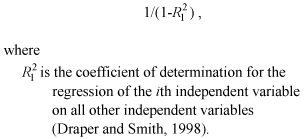
These two terms must be used together to capture and express an annual periodic cycle with an unknown phase offset. Using only the sine or cosine term without the offset is less likely to capture a periodic signal in the data. However, the sine and cosine terms also could cause an interaction with the other independent variables; therefore, the model building is done with and without the sine and cosine terms, and the presence of such interactions is then detected using an F-test (Helsel and Hirsch, 1992; R. Hirsch, U.S. Geological Survey, written commun., December 2008). Sine and cosine terms were tested in regression models for TSS, TP, and E. coli bacteria for the data scenarios that are presumed the most robust input calibration data at the respective sites; that is, Scenario 3 for Fanno Creek and Scenario 2 for Dairy Creek. Data used in this study were initially examined graphically for patterns between potential explanatory variables and the dependent variables. Some patterns that were observed included the presence of bimodal distributions or possible outliers that might affect regressions among the constituents, and correlations (either positive or negative) that might be indicative of predictive signals. Because of their potentially large effect on the regression statistics, outliers were defined as any data points lying more than three times the interquartile range beyond the 25th and 75th percentile values for a particular constituent (Lewis, 1996; Uhrich and Bragg, 2003; Lietz and Debiak, 2005; Rasmussen and others, 2008), and investigated for possible data coding problems, field or laboratory irregularities, or other documented issues that might explain their abnormality. If documented problems could not be corrected, the data were excluded from regression calculations, whereas the data were retained if all available information confirmed the sample integrity. Model building was initially performed with backward, stepwise, linear regressions (Helsel and Hirsch, 1992; SAS Institute, 1989), with an alpha value of 0.05, using either the original or log-transformed data, whichever provided the best fit. When stepwise-regression selected independent variables that were surrogates for each other (for example, untransformed and log-transformed versions of the same variable, or stage and streamflow), one variable was removed and the stepwise process was repeated. However, stepwise regression algorithms tend to continue adding explanatory variables until the coefficient of determination (R2) is maximized, whether or not the added variables actually provide useful information, and can create models that are overfitted (Burnham and Anderson, 2002). Therefore, the initial stepwise regressions were used only as a starting point to evaluate additional model forms using reduced sets of explanatory variables. Subsequent iterations were performed to minimize Mallow’s Cp (SAS Institute, 1989; Draper and Smith, 1998), and used the adjusted-R2, which penalizes additional variables, as a model selection scheme. This process was similar to a “Best-Subsets” regression (Draper and Smith, 1998), although less formal. One challenge when using stepwise regression or other algorithms to select the best correlation was exploring the use of variables in their native units and log transformed forms. Although one might want to evaluate native and transformed variables, inclusion of the forms together introduces opportunities for significant cross correlation or multicollinearity; software programs that automatically perform such algorithms are usually incapable of distinguishing between variables that are truly independent and those that are transformed versions of another variable. The process of model selection by necessity, therefore, was iterative and ultimately was reduced to using log-transformed dependent variables to minimize the possibility that the resulting predicted values would be negative, while evaluating native and transformed versions of the independent variables using the methods discussed previously. Interactions between independent variables, such as occurs if one variable is dependent on another, can reduce the reliability of correlation coefficients (Draper and Smith, 1998), and can contribute to overfitting of regression models (SAS Institute, 1989). The net result tends to be an increase in the standard errors of the independent variables, an effect that is minimized with increased observations. One measure of multicollinearity is the Variance Inflation Factor (VIF), which measures the degree to which the variance of the coefficient of determination for a particular variable is increased because of interdependence between that variable and others in a particular model. The VIF is calculated as
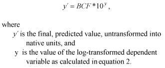
The value of the VIFs are dependent solely on the interactions of the independent variables with each other. Thus, VIFs for a set of independent variables can vary according to datasets used, or in this study, according to scenarios. Likewise, the same dataset may be used in regressions for different dependent variables, and the VIFs would be identical for each identical grouping of independent variables; regressions with only one variable have no interactions and, therefore, no VIF is applicable. The acceptable magnitude of a VIF is dependent on the objectives of a specific study. Several rules-of-thumb for VIFs are sometimes given, and tend to range from greater than 0.2 to less than 10 (Helsel and Hirsch; SAS Institute), but variables with VIFs exceeding these levels may still be useful in a model if they have a low p value. Alternately, a critical value for a maximum acceptable VIF (referred to hereafter as VIFcrit) for an equation can be calculated by substituting the overall coefficient of determination of the model (R2, or in this study, adjusted-R2) for When log-transformed dependent variables are included in regression models, a transformation bias can be introduced when the results are converted back to native units for making predictions. In these cases, a bias correction factor, or BCF (Helsel and Hirsch, 1992) is necessary; the BCF is multiplied by the value of the predicted dependent variable after the BCF is transformed back into native units by taking the antilog. That is,
Duan’s BCF is the average of the residuals of the dependent variable in the regression dataset; when the dependent variable was log transformed, the antilog of the residual was taken before averaging to determine the BCF. Likewise, when log-transformation was used for prediction, the lower and upper 95 percent prediction interval values (SAS Institute, 1989; Helsel and Hirsch, 1992) also were converted to native units with the antilog, and these were corrected using the same BCF as the predicted dependent variables. For the Fanno Creek and Dairy Creek sites, predicted hourly concentrations and their 95 percent prediction intervals were computed for selected water-quality constituents using regression models, and using the indicated hourly monitor and streamflow records as independent variables. Predictions were evaluated against the available validation data (tables 6 and 7) by interpolating the hourly predictions to the time of the validation samples, and then comparing the resulting values to the validation samples using a series of goodness-of-fit statistics (table 8). This validation exercise for the regression models provides an independent measure of the quality of the predictions for the dependent variables and could assist in the decision about which model is the most robust. Not all goodness-of-fit metrics in table 8 are shown in subsequent tables of model results, due to space constraints, but all were used in evaluation of model performance. The available input datasets and resulting regression models were not adequate for making predictions for the non-target sites (table 1), and only the preferred model forms, without the supporting regression coefficients, are presented to provide an indication of the most important independent variables to consider for monitoring. Where regression results seem to provide a reasonable starting point for future modeling, several model forms are shown along with their respective coefficients, diagnostic statistics, and selected goodness-of-fit statistics. Diagnostic statistics include the adjusted-R2 and the root mean square error (RMSE) of the regression. The RMSE assesses the typical error between predicted and observed values. As the root mean square is equal to the square of the mean plus the square of the standard deviation, then if the mean error is zero (no bias), the RMSE is equal to the standard deviation of the errors. The Nash-Sutcliffe Coefficient (Nash and Sutcliffe, 1970), otherwise known as the Coefficient of Model-Fit Efficiency, is one of the goodness-of-fit statistics computed for these models and commonly is used for assessing the accuracy of hydrologic models. Imbalance in the model residuals is assessed by examining the number of negative and positive differences between a model’s predicted results and the comparable laboratory values; a sign test can be used to estimate the likelihood that the residuals were random in the positive or negative directions. Results using several models illustrate the potential explanatory variables and transformations of variables that could be used and the effects of using different input datasets. More detailed regression, neural network, or autoregressive models could be built and would be useful for comparison. This study, however, is meant to be a proof of concept rather than a definitive model building exercise. Simple multiple linear regressions should be sufficient to determine whether adequate information is present in the monitor data to predict TP, TSS, and E. coli bacteria in Fanno and Dairy Creeks. |
First posted June 18, 2010 For additional information contact: Part or all of this report is presented in Portable Document Format (PDF); the latest version of Adobe Reader or similar software is required to view it. Download the latest version of Adobe Reader, free of charge. |

![]() U.S. Department of the Interior | U.S. Geological Survey
U.S. Department of the Interior | U.S. Geological Survey
URL: http://
pubsdata.usgs.gov
/pubs/sir/2010/5008/section3.html
Page Contact Information: Contact USGS
Page Last Modified:
Thursday, 10-Jan-2013 19:11:32 EST

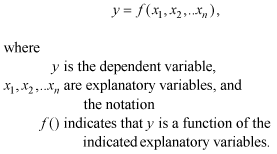 (1)
(1)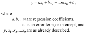 (2)
(2)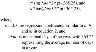
 (3)
(3) (4)
(4)