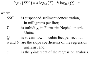
Data Analysis


Suspended sediment, turbidity, and streamflow data from the two Johnson Creek stations were compiled and screened for errors. Several regression models were created for each station and evaluated using diagnostic linear regression statistics. When necessary to provide a complete record, missing data were estimated. The resulting data sets and regression models were used to calculate SSL for water years 2007–10.


Model Data Set


The data used in the regression analyses were compiled from the SSC values of the physical samples and the continuous streamflow and turbidity data at each station. For the Gresham station, 15-min recorded streamflow and turbidity values were averaged during the period when each suspended-sediment sample was collected. In a similar manner, streamflow and turbidity were averaged using the 30-min recorded data for the Milwaukie station.


The suspended-sediment samples were screened for outliers using the methods outlined in Helsel and Hirsch (2002) and Rasmussen and others (2009). Scatter plots of turbidity compared with SSC identified four samples (two from each station) collected on January 31 and March 13, 2008, as potential outliers. Subsequent inspection revealed a laboratory error, and these samples were eliminated from further analysis. Samples also were evaluated for the percentage of suspended sediment finer than 62 µm, which ranged from 88 to 98 percent at Gresham (appendix A), and 81 to 96 percent at Milwaukie (appendix B). An outlier in the percentage of suspended sediment finer than 62 µm might suggest problems with the sample. No samples were removed based on this criterion, and all remaining samples for each station were used in the two regression analyses.


Regression Model Evaluation


Seven linear regression models were evaluated for each station (table 2). Model 6 was selected for use at both stations based on a comparison of diagnostic linear regression statistics and the evaluation of the linear regression model residuals. The two equations selected and the upper and lower model standard percent error (MSPE) are shown in table 3. MSPE is the root-mean squared error expressed as a percentage (Rasmussen and others, 2009). The relation between measured and computed SSC values using model 6 is shown in figure 3. The two stations show similar degrees of fit, and indicate no evident bias for the range of SSC values. A full review of the regression model selection process is available in appendix C.


Estimation of Missing or Erroneous Data


Computation of annual SSL requires complete SSC and streamflow records, in regular time increments. Because streamflow and turbidity were used to calculate SSC, a time series of SSL could not be computed for periods missing streamflow or turbidity data. Turbidity time series for the Gresham and Milwaukie stations were incomplete in all 
4 water years because of sensor fouling or maintenance issues. Gaps in the streamflow records were less common and typically resulted from freezing conditions or instrumentation issues.


Two methods were considered for estimating SSC values during periods of missing streamflow or turbidity data: 
(1) SSC values were estimated directly by performing regressions of SSC against whichever time series were available at the two stations, and (2) streamflow and turbidity values were regressed using the same independent variables. These estimated streamflow or turbidity values then were used to estimate SSC values. Both methods benefit from the high correlations between streamflow and turbidity and between turbidity values at the two stations.


To test the effectiveness of both methods, three periods with complete data sets of streamflow and turbidity were selected—one during a high peak, one during a moderate peak, and one during summer low flow. Turbidity values were assumed to be missing for part of all three periods, and SSC values were estimated using both methods. These estimated SSC values then were compared against the SSC values computed using the equations from table 3, which are considered true values for the purpose of this experiment. The method of estimating SSC values directly tended to underestimate SSC during periods of high flow and overestimate SSC during periods of low flow. Both methods displayed problems with timing during peaks, as turbidity values tend to peak prior to streamflow or SSC values. The second method of estimating streamflow and turbidity was selected based on its relatively higher degree of accuracy. Estimated values of streamflow and turbidity are not saved in NWIS, but are available from the authors upon request.


Missing Turbidity Values


Missing turbidity values were estimated using linear regression analysis and a simple smoothing algorithm. For each missing period, a regression analysis was performed using streamflow and turbidity data from a relatively narrow time frame before and after the missing period. When needed and available, a multiple linear regression was performed using streamflow data from the station with missing data and turbidity values from the other gaging station. For example, no valid turbidity data were recorded at the Gresham station during October 24–26, 2007, due to fouling of the probe. A multiple linear regression model was developed relating the turbidity values at the Gresham station for October 9–23 and October 27–November 13, 2007, to the Gresham streamflow and Milwaukie turbidity values for those same dates. The adjusted coefficient of determination (Adj R²) value of this particular model was 0.71, reflecting the large range in flow and turbidity values and the noise inherent in the turbidity record. Over the 4-year period of this study, this method was used to estimate 35 and 16 percent of the turbidity values at the Gresham and Milwaukie stations, respectively.


The need for continuous turbidity data was most important during autumn and winter, when most suspended sediment was being transported. During summer, warm temperatures and low flow in the stream caused persistent biological fouling of the in situ turbidity probes. Consequently, the probes were removed during the summers of 2009 (Gresham station) and 2010 (Gresham and Milwaukie stations), and re-installed in autumn of those same calendar years. As a result, no turbidity data were recorded at either station during the unexpected June 2010 high streamflow. To estimate turbidity during this period, the regression models were developed using longer time-series variables, encompassing streamflow ranges equal to the high streamflow. The turbidity values estimated during the late spring to early autumn periods account for more than 80 percent of the total number of turbidity values estimated. 


Missing Streamflow Values


Streamflow records were nearly complete for both stations. The Gresham and Milwaukie stations were missing 0.9 and 0.2 percent of streamflow values, respectively. Additionally, 90 percent of missing streamflow data occurred during summer, when streamflow typically varies little and is easiest to estimate. Incomplete streamflow time series commonly were the result of equipment malfunction or routine maintenance. Missing streamflow records were estimated by creating regression models with streamflow records from the other gaging station, and using a simple linear smoothing algorithm. The time series of the downstream station (Milwaukie) was shifted 4 hours to account for time of travel between the two stations, based on an evaluation of which time lag provided the largest coefficient of determination between the two stations. Regression models for streamflow estimation proved to be more accurate than for turbidity estimation, with adjusted R² values ranging from 0.96 to near 1.0.


The final time series of streamflow and turbidity at the Gresham and Milwaukie stations are shown in figures 4 and 5, respectively. Estimated streamflow data were not included in figures 4 and 5 because data were insufficient and do not show clearly. There is a slight lag between turbidity and streamflow, but the overall shapes of the hydrographs typically are similar.


Computation of Suspended-Sediment Concentration


As described in the section “Data Analysis,” regression models were developed to compute continuous SSC time series for each station using the discrete SSC, streamflow, and turbidity data associated with each suspended-sediment sample. The selected regression model equation form was:


(1)


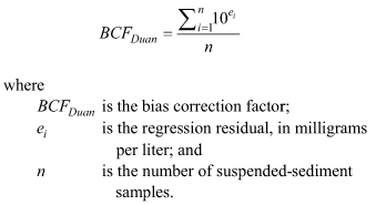
The continuous time series of streamflow and turbidity for each station were input into the equations in table 3 to produce a time series of SSC values for water years 2007–10. The transformation of the resulting SSC values from log to arithmetic space results in a bias of the data (Helsel and Hirsch, 2002). This bias can be reduced by multiplying each SSC value by a bias correction factor (BCF), also known as a “smearing estimator.” The Duan BCF (Duan, 1983) was computed as follows:


(2)


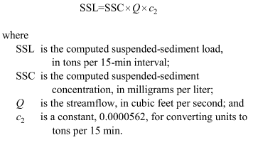
BCF values used are listed in table 3.


Computation of Suspended-Sediment Discharge and Load


The annual SSL was computed for each station for water years 2007–10. For the Gresham station, computed 15-min SSC, in milligrams per liter, and corresponding streamflow values, in cubic feet per second, were used to calculate SSL, in tons per 15 min using the following equation:


(3)


Similarly, SSL was computed for the Milwaukie station in tons per 30 min using the following equation:


(4)


The daily SSL was computed by summing the 96 or 48 computed 15- or 30-min SSL values per day for Gresham and Milwaukie stations, respectively. The monthly and annual SSL were computed by summing the appropriate daily SSL values. Daily totals of SSL are termed “daily values.” The individual 15- or 30-min values for the Gresham and Milwaukie stations are termed “unit values.”


First posted October 3, 2012