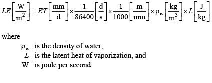
Methods of Study


Evapotranspiration (ET) of water is an important component of the hydrologic cycle. Globally, ET is equal to precipitation (P), and over land, ET is about 62 percent of P (Brutsaert, 1982, table 1.1), larger than any other terrestrial hydrologic component. The importance of ET is underscored by recognizing that once water evaporates into the atmosphere, it is no longer available for human consumption until it returns to the surface as P, which led to the adoption of the term consumptive use as a synonym for ET. Although the ratio ET:P decreases in humid climates (generally reducing the importance of ET there), ET:P approaches unity as aridity increases, making ET extremely important in semiarid and arid parts of the world.


The word evapotranspiration was coined in the 1930s to combine the processes of evaporation and transpiration into a single term (Brutsaert, 1982). Whereas evaporation is the phase change of liquid water to water vapor, transpiration is evaporation that specifically occurs within the substomatal cavities of vegetation. Plants withdraw soil water and nutrients from the root zone and transport them up through the plant stems to the leaves, where the nutrients are used by plant tissues and the water evaporates through microscopic holes in the leaves called stomata. Current usage of ET refers to the sum of evaporation from open water, wet plant and mineral surfaces (such as shortly after rainfall), sublimation from snow and ice, and transpiration. In this report, ET refers to water loss from vegetated sites to the atmosphere, and evaporation (E) is reserved for water loss from extensive open-water sites to the atmosphere. Both ET and E can be expressed in a variety of units. In this report, daily and biweekly totals are expressed in millimeters per day (where millimeters is depth of liquid water per unit area of land surface); these basic units are aggregated into meters per year to describe annual evaporative losses.


Evaporation of water consumes a relatively large amount of energy, known as the latent heat of vaporization of water, L. Consequently, ET is a substantial component of the energy balance of the Earth’s surface, as well as the hydrologic balance. As liquid water vaporizes at the surface, it carries energy into the atmosphere, which is released at some later time when the vapor re-condenses into liquid. 


The rate of energy used to sustain a given ET rate is known as the latent-heat flux (LE) and is equal to:


     (1a)


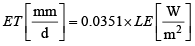
Both ρ_w and L are very weak functions of temperature, and they are roughly constant over the range of temperatures encountered in this study. Therefore equation 1a can be rewritten approximately as:


     (1b)


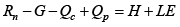
Energy Balance of a Vegetated or Open‑Water Surface


Virtually all of the energy arriving at the Earth’s surface originates from the sun (Kiehl and Trenberth, 1997). On a global, annual average basis, solar (short-wave) radiation arriving at the top of the atmosphere is 342 watts per square meter (W m^-2), and is reduced to 198 W m^-2 at the Earth’s surface. On average, 168 W m^-2of the solar radiation arriving at the surface is absorbed, and 30 W m^-2 is reflected, giving an average reflectivity (a, also known as albedo) of 0.15. Some of the solar radiation arriving at the top of the atmosphere is reflected to space (77 W m^-2) or absorbed by the atmosphere (67 W m^-2). Atmospheric absorption occurs primarily by clouds, water vapor, dust, trace gases, and aerosols. The absorbed energy heats the atmosphere, which in turn emits long-wave (infrared) radiation, some of which arrives at the surface. The surface either reflects or absorbs this long-wave radiation, and also emits its own long-wave radiation. The processes of reflection, absorption, emission, and transmission of long-wave radiation between the surface and atmosphere are complex, but on average, the net long-wave exchange is 66 W m^-2 from the surface upward to the atmosphere.


At the Earth’s surface, the algebraic sum of incoming solar radiation (positive), reflected solar radiation (negative), incoming long-wave radiation (positive), and outgoing long-wave radiation (negative) constitutes net radiation, R_n. On average, R_n is (198 minus 66, or) 102 W m^-2 (Kiehl and Trenberth, 1997) and drives all of the other (nonradiative) energy exchanges at the surface. A schematic of the typical daytime energy balance of a vegetated surface is shown in fig. 2A. The surface typically warms during the day in response to the input of energy from R_n. Some of that energy moves into the subsurface by conduction, known as the soil heat flux, G. 


The portion that warms the vegetation biomass is canopy storage, Q_c. On most days, absorbed radiation warms the vegetation and soil surfaces above the temperature of the overlying air, giving rise to turbulent transfer of heat into the air, known as sensible-heat flux, H. Water evaporating from the surface carries with it the latent-heat flux, LE, another turbulent flux from the surface to the air. Global annual average values of H and LE are 24 and 78 W m^-2, respectively. Finally, the excess heat content of precipitation above the surface temperature produces a typically small flux, the heat of precipitation, Q_p. Adopting the sign convention shown in figure 2A, the surface energy-balance equation can be written as:


     (2)


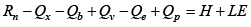
The left side of equation 2 is called the available energy (AE), and the right side is the turbulent flux (TF). In many settings, Q_c and Q_p are minor terms, leaving R_n, G, H and LE as the four main components of the energy balance. In this study, Q_c and Q_p were determined to be negligible and are not included in the calculations.


At night, solar radiation terms become zero and outgoing long-wave radiation typically exceeds incoming radiation, causing R_n to become negative. Usually, the surface cools faster than the overlying air due to this long-wave emission, creating a temperature inversion in the air, leading to a sign change in H and a downward flux of sensible heat. Typically, the surface is also cooler than the subsurface soils, and G similarly changes sign. Outgoing night-time G is comparable to incoming daytime G, and long-term values of G approach zero. Most plants close stomata at night, shutting off transpiration, and due to the lack of available energy and colder temperatures, evaporation from soil also approaches zero, resulting in a surface LE that approaches zero at night. If the surface cools below the dew-point, water vapor in the air deposits as dew (or frost when the surface is below freezing) and LE becomes slightly negative.


The dynamic changes in the major fluxes between day and night result in typical 24-hour time series of flux resembling sinusoidal waves, with maxima near solar noon and minima near midnight. Daily average amplitudes and means are greatest in summer and least in winter. In addition, substantial variability about the average patterns occurs, caused by changes in the amount of cloud cover, green vegetation, water availability, wind speed, and atmospheric properties.


The surface energy balance shown in figure 2A is a one‑dimensional, vertical model, written for a specific, uniform surface of interest. Energy balances can vary substantially from one surface type to another. Because the turbulent fluxes are measured at some height above the plant canopy, the assumption is made that they are equal to the values at the surface, corrected for any change in heat or vapor storage between the canopy and the sensor. This assumption is valid if the horizontal extent of the uniform surface of interest in the upwind direction (the fetch) is sufficiently large that the air passing by the turbulent flux sensors has equilibrated to the surface of interest. Consequently, turbulent flux sensors typically are deployed in the midst of a large expanse of a uniform surface type. Tests are available to evaluate the adequacy of the fetch (Schuepp and others, 1990; Stannard, 1997) and are used in this study.


Compared to the energy balance of a land surface, the balance of an open-water surface is complicated by the subsurface transfer of heat in three dimensions as the bulk liquid water mixes in response to wind, density gradients, inflows, and outflows. In addition, solar radiation typically penetrates the water column to some depth, further complicating the subsurface energy exchange. To avoid the problems of measuring the near subsurface energy input, the entire water body is taken as a control volume, and energy fluxes into and out of that volume (rather than a surface) are conceptualized and measured (fig. 2B). The fluxes of R_n, H, LE, and Q_p are analogous to those occurring over land. The flux of heat energy exchanged between the surface and subsurface (the equivalent of G on land) is recast as a change in heat stored in the water body, Q_x, measured by changes in temperature profiles through the water column (Anderson, 1954; Sturrock and others, 1992). If the water body is relatively shallow, heat exchange also may occur between the water and the lake bottom sediments, designated as Q_b. Water bodies also are often connected to streams and groundwater, which can add or remove heat to or from the water body through advection, designated as Q_v. Finally, heat can be added or removed to or from the water body by the evaporating water, depending on whether that water is cooler or warmer, respectively, than the mean water-body temperature. Designated as Q_e, this small flux also occurs over land but is seldom evaluated there because the temperature of the evaporating water usually is not known. The resulting energy balance of a water body can be written as (Anderson, 1954):


     (3)


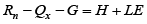
The diurnal behavior of energy-balance fluxes is quite different over water than over land, primarily because (1) solar radiation partially penetrates the surface, (2) the thermal inertia of water is much greater than that of land, and (3) water availability at the water surface is always 100 percent. These factors combine to create a daytime balance where heating of the water surface from R_n occurs more slowly than heating of the land (or vegetation) surface, moderating surface temperature compared to temperature over land. Usually the overlying air heats more quickly than the water surface, resulting in a temperature inversion and a downward (negative) H during the day. Rather than being partially converted into a positive H as over land, R_n (aided by a downward H) drives a large value of Q_x by storing heat at depth in the water column, and the residual energy is partitioned into LE. At night, the air cools faster than the water surface, and H becomes positive. Even though R_n is negative, heat comes back out of storage from the water column (Q_x > -R_n), driving both a positive LE and a positive H. Daytime Q_x over water is a large fraction of R_n, whereas G + Q_c usually is a small fraction of R_n over a densely vegetated canopy on land. The 24-hour wave-like behavior of H over water is about 12 hours out of phase with H over land, and magnitudes are much smaller. The 24-hour behavior of LE over water is less wave-like, tending toward a more constant (positive) value fluctuating about the 24-hour mean.


The two wetland sites of the current study exhibit energy‑balance characteristics of both the vegetated land surface and the water body described in the previous several paragraphs. Between midsummer and midwinter, standing water is not present at the sites, and the surface behaves purely as a vegetated land surface. From midwinter to midsummer, water depth at the sites typically increases to as much as about 0.8 m, is maintained at that level for about 2 months, and then recedes back to zero. During this period, diurnal energy flux patterns are intermediate between those of a vegetated land surface and an open-water body, depending on vegetation status and water depth. The energy balance of a wetland surface with standing water contains elements of equations 2 and 3, and can be written:


     (4)


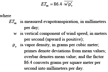
At times when standing water is present, the dense vegetation canopy effectively inhibits significant lateral exchange of energy in the water column, and therefore Q_v is assumed to be zero. At times when standing water is not present, Q_x and Q_v are both zero.


Eddy-Covariance Measurements of Latent- and Sensible-Heat Flux


Turbulent exchange of energy and mass in the lowest layer of the atmosphere, the atmospheric boundary layer (ABL), occurs through eddy diffusion (Brutsaert, 1982, p. 52–56). Above a flat, level surface, the mean air movement is commonly recognized as being horizontal and is quantified as wind speed. However, superimposed on the mean wind are random turbulent upward and downward motions, resulting in instantaneous wind vectors with non-zero vertical components. The interplay between air viscosity, geostrophic wind (wind at upper levels of the atmosphere caused by regional pressure differences), surface heating, and surface roughness creates an ABL where air motions tend to aggregate into blobs or eddies which span a wide range of sizes, from centimeters to kilometers. Within an eddy, movements are highly correlated and can be quite distinct from those in nearby eddies. Similarly, concentrations of admixtures (for example, the heat, water vapor, or carbon dioxide content) may vary from eddy to eddy. Vertical transport of eddy admixtures results from the vertical components of eddy motions, a process similar to molecular diffusion but on a much larger scale. As an eddy moves upward or downward, it carries the admixtures along with it, giving rise to vertical turbulent flux. Above an extensive uniform surface, the net vertical transport of an admixture is equal to the algebraic sum of the transport contributions from all eddies (or a statistically significant sample thereof) passing over the surface. Thus, over an evaporating surface, upward-moving eddies contain, on average, more water vapor than downward-moving eddies. If certain criteria are met, the flux of an admixture can be measured through a high-speed bookkeeping of vertical eddy motion and admixture concentration, known as eddy covariance (EC). In the case of water vapor, the EC equation takes the form (Dyer, 1961):


     (5)


The quantity is the covariance of w and ρ_v. Similarly, the equation for sensible heat is:


     (6)


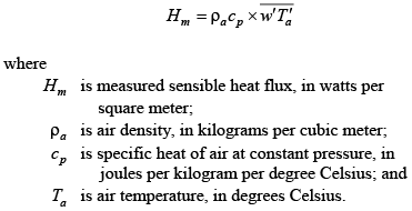
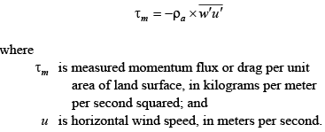
Typically, means are computed over 20 to 60-minute periods, and deviations from means are measured 5 to 20 times per second.


In addition to turbulent flux of heat and mass between the surface and atmosphere, a turbulent flux of horizontal momentum also occurs from the atmosphere to the surface. Horizontal wind speed is zero at the surface and increases with height above the surface—a wind-speed profile that indicates greater momentum at height, decreasing to zero momentum at the surface. This gradient implies a flux of horizontal momentum from the upper atmosphere downward to the surface, also recognized as a drag force exerted on the surface by the air. The transfer of momentum downward occurs through eddy diffusion and can be expressed as:


     (7)


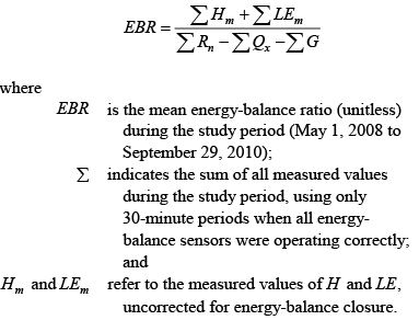
Usually, τ_m is measured concurrently with ET_m and H_m because it is needed to calculate corrections to those fluxes.


The Energy-Balance Closure Problem


The surface energy balance illustrated in figure 2A and quantified in equation 2 accounts for all significant energy fluxes to and from a surface that are currently recognized (Wilson and others, 2002). Commercially available instrumentation provides measurements of each term in equation 2 separately. If all measurements are accurate and all significant fluxes appear in equation 2, then the left side of the equation, the available energy (AE), should be equal to the right side, the turbulent flux (TF), within the limits of measurement accuracy. This concept is commonly called energy-balance closure. Graphical and statistical comparison of AE with TF frequently is used to identify problems associated with sensor inaccuracies and malfunctions, sensor deployment, insufficient fetch, or complex terrain. Due to random components of some errors, measurement accuracy usually increases as the accumulated time interval of continuous measurements increases. In addition, some errors may be systematically linked to time of day or year, but are largely self-compensating when the measurement interval is a full day, a number of full days, or a full year. Consequently, energy-balance closure usually is evaluated over longer time periods, preferably a year or multiple years.


Comparisons of long-term AE with TF from many studies display a chronic mismatch between the two. The ratio of TF to AE generally ranges from about 0.6 to 1.0, it most frequently is around 0.7 to 0.8 (Twine and others, 2000; Wilson and others, 2002; Foken, 2008). In the past, undermeasurement of TF (Dugas and others, 1991; Twine and others, 2000; Gash and Dolman, 2003) or overmeasurement of R_n (Campbell, 1980; Halldin and Lindroth, 1992; Bossong and others, 2003), both presumably caused by instrumental performance or deployment, have been suggested as reasons for the mismatch. Soil-heat flux and storage terms are not suspect because long-term measured values approach zero, consistent with principles of environmental physics. Recently, Foken (2008) argued that current instrumentation and field practices are now sufficiently accurate that they can no longer account for the lack of closure. Rather, Foken proposed that land-surface scales of heterogeneity on the order of 1 to 10 km may generate large-scale eddies that contribute to turbulent flux in a fashion that is unlikely or impossible to be fully measured using the EC method. Foken argues that the time of passage of these very large eddies may be too long for typical averaging periods (which are 30 minutes to 1 hour; longer averaging periods violate the stationarity principle) to capture. Further, he suggests that the large eddies cluster near substantial changes in land-surface type (the very locations that are avoided as measurement sites if the goal is to obtain a clear, unambiguous flux signal from a surface of interest), inducing undetected horizontal flux advection over the central areas of homogenous land-surface patches, where sensors typically are deployed. Large-scale (~5 km) scintillometer measurements of turbulent flux and large eddy simulation modeling results support these ideas, both indicating adequate energy-balance closure when applied to horizontal scales of several kilometers encompassing changes in land-surface type (Foken, 2008). Although a proven remedy for ordinary EC data collection is not offered, Foken suggests as a first guess closing the energy balance by adjusting both H and LE, maintaining the ratio between them (H/LE = β, the Bowen ratio). This method has also been used commonly in the past (Barr and others, 1998; Blanken and others, 1998; Twine and others, 2000) when energy-balance closure was not obtained. Although Foken’s (2008) ideas are promising, the scientific community is still undecided on the answer to the energy‑balance closure problem.


In this report, measured H and LE are corrected using the energy-balance closure principle. A single value of the energy‑balance ratio is computed as:


     (8)


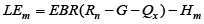
First, gap-filling and standard corrections (described in Eddy‑Covariance Data Processing) are applied to the 30-minute H and LE data. Then the resulting H_m and LE_m values are divided by EBR to obtain final 30-minute values that produce long-term energy-balance closure. The use of a single, mean value of EBR, rather than multiple values calculated over shorter periods, is discussed in Energy‑Balance Closure and Trends. The EBR values at both EC sites are reported in Energy-Balance Closure and Trends, allowing the reader to compute H_m and LE_m (or ET_m) if desired. Applying this EBR correction to the measured wetland EC fluxes facilitates direct comparison with measured open-water evaporation, which is based on the concept of full energy-balance closure.


Eddy-Covariance Sensors and Data Collection


The EC method requires fast-response sensors to adequately measure the rapid fluctuations in wind-speed components, air temperature, and vapor density caused by movement of the smallest eddies that contribute to the turbulent flux of momentum, heat, and water vapor. Two specialized sensors developed for eddy-covariance measurements by Campbell Scientific were used in the present study. A 3-axis sonic anemometer (Model CSAT3) measured wind vectors along three measurement paths, all at 60 degrees (°) from vertical, and at 120° from each other in the horizontal plane (fig. 3). The sensor was leveled in the field by means of a sensitive bubble level. Software in the CSAT3 converted the measured vectors into 3 orthogonal vectors aligned with the sensor’s major axes (one vertical and two horizontal). The CSAT3 measured the wind vectors by sending ultrasonic signals between transducer pairs (fig. 3), measuring the travel time, and using the Doppler effect to compute the wind speed. The two orthogonal horizontal vectors were used to compute the resultant horizontal vector (u) appearing in equation 7. The CSAT3 also measured sonic air temperature, T_s, using the dependence of the speed of sound on temperature. This sonic air temperature is slightly different than true air temperature, T_a, and requires a small correction to obtain the covariance (eq. 6), described in Eddy‑Covariance Data Processing. A krypton hygrometer (Model KH20) was deployed adjacent to the CSAT3 to sense vapor density fluctuations (fig. 3). The source tube emits a krypton radiation signal through a window, along the short (1 cm) measurement path, and through another window to the receiver tube. Because the radiation is absorbed by water vapor, the signal strength received is inversely proportional to the vapor density in the measurement path, providing a virtually instantaneous measure of .


The EC sensors were deployed from a galvanized steel tripod and were oriented to minimize interference upwind of the measuring paths during wind flow from the prevailing directions. The tripod was installed immediately adjacent to a platform structure that supported all of the other sensors and hardware and provided a working surface during installation and site visits (fig. 4). Isolation of the tripod from the platform prevented disturbing the EC sensors while researchers were moving about on the platform during site visits. The platform and tripod required special modifications to obtain adequate support from the spongy peat soil underlain by gyttja. Slow settling of the structures into the peat could affect sensor levels unacceptably, and penetration into the semiliquid gyttja below could topple the entire station. Large wooden feet made from 2 by 10-inch treated lumber were attached to the bottom of the tripod legs—and to the platform legs with additional sections of leg protruding below the feet to puncture the peat layer and anchor the platform (fig. 5). This design was sufficient to prevent any noticeable differential settling of the structures, thereby maintaining sensors level within acceptable limits between site visits. The EC sensors were set at heights of 3.61 m and 3.76 m above land surface at the bulrush and mixed sites, respectively. At both sites, the KH20 measurement path was located 10 cm from the midpoint of the CSAT3 measurement paths (fig. 3).


The response times of the CSAT3 and KH20 sensors are nearly instantaneous, ensuring that rapid sampling of their outputs accurately tracks the random variations in wind, temperature, and vapor density. All 5 EC variables (three orthogonal wind vectors, sonic air temperature, and vapor density) were sampled at 10 hertz (Hz), using a Campbell Scientific CR1000 data logger. The 10 Hz data were temporarily stored in the data logger during each 30-minute period. These data were then used by the logger to compute means and standard deviations of each variable and all (10) of the possible covariances between variables (using block averaging) at the end of each period. In addition, a time stamp (year, month, day of month, hour, minute), preliminary flux values, wind direction, data-logger temperature, system battery voltage, and sensor diagnostics were recorded at the end of each period. Data were sent automatically via cell phone modem to the USGS Water Science Center in Portland, Oreg., daily. At each site, power was supplied from a single 40 W solar panel, with storage initially provided by a 100 ampere‑hour deep cycle flooded battery (fig. 4). Subsequently a second battery was added at each site after night-time low-power problems occurred at the mixed site.


Eddy-Covariance Data Processing


Although the EC method is the most direct measurement of turbulent fluxes between the surface and atmosphere currently available, the apparent simplicity of equations 5 through 7 is slightly complicated by the need for minor corrections arising from limitations of the method and sensors. The following commonly used corrections were applied to EC data in the present study.


First, the use of in equations 5 through 7 is predicated on the assumption that mean wind flow past the sensors is horizontal (that is,  = 0). Over surfaces with uneven topography, vegetation, or heating, 30-minute mean wind vectors may not be horizontal, and the 30-minute mean vertical component may change depending on wind speed, wind direction, and solar heating. Although land surface at both EC sites was very flat and level, disturbances to the vegetation occurred from station installation and from wind gusts that lodged patches of bulrush and cattail, creating depressions in the canopy in the vicinity of the stations. Coordinate rotation was, therefore, performed to correct the three covariances in equations 5 through 7 (Tanner and Thurtell, 1969). This correction requires computing second‑order moments and may increase or decrease the calculated flux, depending on the vertical direction of the rotation. Rotations were made based on the 30-minute mean wind vector, rather than using the long-term planar fit method (Paw U and others, 2000), which is more appropriate when the land surface or the sonic anemometer is not level.


Second, above even a flat, level surface, a more subtle effect contributes to a nonzero when H ≠ 0, caused by the inverse relation between air temperature (T_a) and density (ρ_a) at constant pressure. For example, if H > 0, rising eddies are warmer and, therefore, less dense than sinking eddies. Because the vertical flux of dry air over a horizontal surface is zero, a small (upward) > 0 occurs to maintain conservation of mass (Webb and others, 1980), and the converse occurs ( < 0) when H < 0. A correction to the measured (eq. 5) was made to remove the effect of 
 ≠ 0 following Webb and others (1980). This correction increases ET when H > 0 (usually daytime) and decreases ET when H < 0 (usually nighttime), generally producing a net increase in daily ET.


Third, a small correction to the measured covariance in equation 5 is needed because the krypton radiation emitted by the KH20 source tube is slightly attenuated by oxygen, and oxygen density is proportional to total air density. At constant pressure, warmer eddies are less dense, creating a small error in the measured when H ≠ 0. Following Tanner and Greene (1989), a correction proportional to H was made to the measured , to remove this artifact.


Fourth, the sonic air temperature, T_s, is slightly different than true air temperature, T_a, because T_s is affected by the water vapor content of the air. Following Schotanus and others (1983), a small correction proportional to LE was made to convert to . Because the second, third, and fourth corrections are interdependent, these corrections were iterated until convergence was obtained.


Fifth, frequency response corrections (Massman, 2000) were made to compensate for the inability of the EC method to record flux contributions from the largest and smallest eddies under certain conditions. The largest eddies contributing to flux may require longer than 30 min to pass by the sensors in low wind speeds (less than about 0.5 m/s). However, averaging periods longer than 30 min begin to violate the stationarity principle and are generally not used. At the other extreme, contributions to flux from the smallest eddies (about 10 cm) may not be fully recorded due to sensor geometry such as path-length averaging and sensor separation. These corrections apply to H, LE, and τ and the corrections to each flux depend on the magnitudes of the other fluxes, so these corrections also were iterated until convergence was obtained.


The calibration factor of the KH20 varies slightly with ambient vapor density, ρ_v. The manufacturer supplies the calibration curve data points, and the slopes of least squares linear regression fits to the data in the high and low ρ_v ranges. The manufacturer suggests using one or the other slope as the calibration factor, depending on ambient ρ_v. This approach creates unnecessary discontinuities at the transition and small errors in computed ET. We improved upon the piecewise linear approach by fitting a cubic polynomial to the calibration data (r ² > 0.999) and using a more exact calibration factor for each 30-minute period, equal to the slope of the cubic curve (a quadratic function of ρ_v).


Fully processed 30-minute ET and related data are aggregated into longer period averages and totals for presentation, seasonal analysis, comparison with other work, and computation of crop coefficients. Depending on the application, periods of 1 day, 2 weeks, a growing season, or 1 year are used as averaging periods.


Gap-Filling Missing or Bad Eddy-Covariance Data


The EC sensors can malfunction when their measurement paths or surfaces are obstructed by water droplets, water films, snow, ice, particulates, leaves, insects, webs, avian fecal matter, or other solids or liquids that interfere with the transmission or reception of the sensor signals. By far, the most common interference during this study occurred from precipitation, and it affected primarily the KH20 hygrometer. The CSAT3 sonic anemometer also was affected at times by the presence of liquid or solid water, but much less frequently than the KH20 hygrometer. Once the measurement paths and surfaces of either sensor are sufficiently free of water and other foreign matter, correct sensor operation and data collection resume.


Periods of invalid data were identified by graphing the four energy-balance fluxes, precipitation, air temperature, vapor density, the KH20 voltage signal, horizontal wind speed, and momentum flux for periods of a week and searching for anomalous patterns in H, LE, and τ. Anomalous patterns in H and LE (extended periods of zero flux, spikes, noise) were identified based on energy-balance principles. Periods of suspect data were then graphed on an expanded time scale (1 or 2 days per graph) to identify invalid data by 30-minute intervals. In almost all cases, reasons for invalid flux data were identified by inspection of the auxiliary data from the same period. For example, recorded precipitation, a sudden decrease in the KH20 voltage signal without a corresponding increase in vapor density, and relative humidity near 100 percent, were commonly noted during invalid flux data collection and strongly suggested that water interfered with one or both EC sensors.


Based on the close inspection of flux and auxiliary data, flags were added to data records to indicate: (1) invalid data, (2) which fluxes were affected, and (3) the appropriate gap-filling method to use. By inspection, it was found that the status of H and τ (operational or invalid) were identical, requiring only a single flag to indicate the status of both fluxes. Gap-filling was accomplished through linear interpolation or through energy-balance modeling. Linear interpolation was used when the gap was sufficiently short (≤ 2 hours) or the auxiliary data suggested that the missing flux varied approximately linearly between the last valid data point before the gap and the first valid data point after recovery. During the growing season, this second condition typically was restricted to periods of 8 hours or less because the diurnal cycle typically imposes a curvature in energy-balance fluxes during longer periods. During winter, periods as long as 18 hours were interpolated if the data indicated low sunlight (overcast), cold temperature, and precipitation—a winter storm. This practice is reasonable because with little diurnal variation in available energy, little resulting diurnal variation in turbulent flux occurs, creating extended periods when H and LE are small and relatively constant. Energy-balance modeling was required to gap-fill LE data only, because all gaps in H and τ were sufficiently short to gap-fill using linear interpolation. Energy‑balance gap-filling of LE incorporated the concepts embodied in equations 4 and 8, and took the form:


     (9)


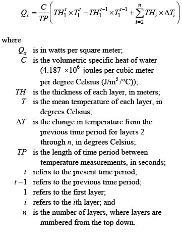
This method estimates LE using the energy-balance closure principle (eq. 4), modified by the observation that the long‑term ratio of measured turbulent flux to available energy (that is, the EBR) usually is less than one (eq. 8).


Periods of missing data occurred at the mixed vegetation site, caused by inadequate battery storage during June 14–25, 2008, and by cell-phone malfunction during July 30–August 12, 2009. The first incident was a series of 13 night‑time gaps, separated by daytime periods of successful data collection when adequate power was supplied directly from the solar panel. The second gap was a 13.1-day period of no data collection. During the low battery power gaps, both EC and meteorological data were missing, whereas during the cell-phone gap, only EC data were missing. Because the two EC sites are of similar land cover and are separated by only 5.8 km, energy fluxes and most weather conditions are very highly correlated at the two locations. Periods of missing data at the mixed site were, therefore, gap-filled using simple linear regression against the equivalent data collected at the bulrush site. The linear relations were established using periods immediately before and after each gap, when data collection at both sites was successful. The periods before and after the gap were each about one-half the length of the gap, or longer. In the case of the recurring night-time gaps, round-the-clock data collected before the first occurrence of low power and after the problem was remedied were used to create robust regressions (exploiting the full diurnal range in flux), even though only night-time periods were gap-filled.


Meteorological, Energy-Balance, and Biophysical Measurements at 
Eddy-Covariance Sites


Meteorological and Energy-Balance Sensors and Data Collection


In addition to basic EC data collection, sensors were deployed at both EC sites to measure meteorological and energy-balance variables: (1) to help identify times when EC sensors were inoperative due to environmental moisture (rain, snow, ice) or other interference; (2) to gap-fill compromised EC data during these times; (3) to evaluate the degree of energy-balance closure; (4) to associate ET and energy‑balance results with environmental conditions; and (5) to evaluate the fetch at the EC sites. Variables measured were net radiation, soil-heat flux, wind speed, wind direction, soil water content, rainfall, air temperature, relative humidity, and water temperature at various depths (when standing water was present). Sensor make and model, measurement height, scan interval, and summary statistics are presented in table 1.


The summary interval for all sensors except the water‑temperature sensors was 30 min. The summary interval for the water temperature sensors was 15 min. The CNR1 net radiometer consisted of four separate sensors to measure incoming solar, reflected solar, incoming long-wave and outgoing long-wave radiation. The rainfall gage was a nonheated tipping bucket and, therefore, did not accurately record snowfall. Small snowfall amounts were recorded upon melting, but they were diminished slightly by any sublimation in the interim. Large snowfall amounts could overtop the gage and be substantially undermeasured. Because the rainfall data were used primarily to determine times when the EC sensors were affected by water, these limitations in the snowfall record were relatively unimportant. The Vaisalla HMP45C temperature-humidity probe and the RM Young 03001 wind speed and direction sensors were deployed to measure wind, temperature, and humidity data even though the EC sensors (CSAT3 and KH20) nominally measure these variables because: (1) gaps exist in the EC data record caused by precipitation or other interference; and (2) the KH20 hygrometer accurately senses rapid deviations from mean ρ_vonly—it does not accurately sense mean ρ_v. The standard, non-EC sensors provided a continuous and accurate record used in troubleshooting and computing small corrections to EC data.


Meteorological and Energy-Balance Data Processing


Saturated vapor pressure (e_s, kPa) was computed from measured air temperature (T_a) using the algorithm of Lowe (1977). This is the maximum amount of water vapor the air can hold, and it increases with increasing temperature. Actual vapor pressure (e, kPa) was computed from e_s and measured relative humidity (RH, percent) as: . Vapor density (ρ_v, g/m³) is the mass of water vapor per unit volume of air and was computed from e using the ideal gas law: where M_w is the molar weight of water (18.0153 g/mol), R is the universal gas constant (0.0083145 kPa (m³/mol)/K), and T_k is air temperature in kelvin.


Mean atmospheric pressure (P, kPa) was calculated using the atmospheric scale height equation: where P₀ is mean atmospheric pressure at sea level (101.33 kPa), z is site altitude (m), and 8434.4 is the scale height of the atmosphere (m). Air density (ρ_a, g/m³) was calculated as the sum of dry air density (ρ_d, g/m³) and vapor density (ρ_v): where and M_d is the molar weight of dry air (28.97 g/mol). Specific humidity (q, g H₂O/g air) is the mass of water vapor per unit mass of air, and was calculated as . Specific heat of air at constant pressure, c_p (in joules per kilogram per degree Celsius), was calculated as the weighted average of the specific heats of dry air (c_pd) and water vapor (c_pv) at constant pressure: (Brutsaert, 1982, p. 43). Quadratic expressions were fit to tabulated data given for c_pd and c_pv(Garratt, 1992, p. 285; Engineering Toolbox, 2011), which vary slightly as a function of temperature.


Wind speed measured with a cup anemometer and wind direction measured with a vane at 1 Hz were processed using data-logger software to compute mean wind speed (U_cup) and mean wind direction (WD) each half hour. Each 1-second U_cup and WD were combined to produce a wind vector, and the 1-second wind vectors were added in vector fashion to compute the resulting half-hour summaries.


Soil-heat flux, G, was measured directly using a soil‑heat flux plate (HFT3, table 1) buried at about 2 cm beneath the soil surface. Any change in energy storage in the soil above the plate was assumed to be negligible. The plates were not buried at the beginning of the study due to the depth of standing water at that time. Scheduled site visits did not correspond to the cessation of standing water, so the plates were buried during the next visit after cessation. This late installation created a period of about 25 days in mid-2008 when G was unmeasured. Later data indicated that when water depth exceeded about 20 cm, G ≈ 0. A model of G was created to fill in the missing data during 2008 when water depth was less than 20 cm. G was modeled as a linear combination of current and past R_n and T_a, using data from times of similar water depth during 2009 when the plate was operational. Candidate past values of R_n and T_a included 30-minute data from the previous 7 half-hours, and the mean from the past 24 hours. Multiple linear stepwise regression was used to select the subset of variables at each site that were significantly related to G. Root-mean-squared errors (RMSE) of the two models were 8.7 and 2.1 W/m² at the bulrush and mixed sites, respectively. Coefficients of determination (r ²) were 0.78 and 0.94, respectively.


When standing water was present, change in energy stored in the water column, Q_x, was calculated from temperatures measured at various depths in the water column. Temperature sensors were located at nominal heights of 0.01, 0.27, and 0.52 m above the soil surface, and (floating) at the water surface (table 1). These sensors divided the water column into layers and the change in heat content of each layer was computed. The value of Q_x was computed as the sum of the change in heat stored in each of the layers:


     (10)


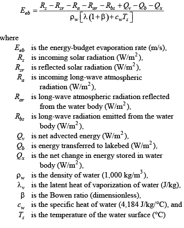
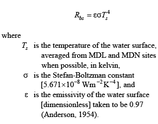
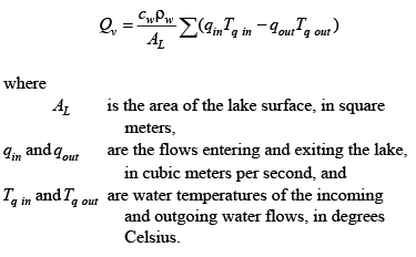
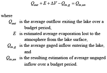
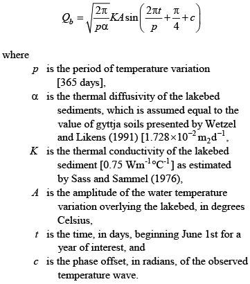
Each layer is bounded by temperature sensors at the top and bottom of the layer, and the mean temperature of the layer is set equal to the mean of the upper and lower sensors. This formula accounts for a change in thickness of the top layer caused by a change in lake level during the time period and assumes lower layers are constant thickness. As water level varied and fixed sensors became exposed or submerged, the value of n changed accordingly. This formula was applied to time periods of 30 min.


Gaps in the Q_x record occurred for two reasons: (1) the sensors were not deployed early enough each year to record the onset of inundation by the rising water; and (2) at times the floating sensor would become entangled in vegetation as the water level receded, causing the sensor to be suspended in air, invalidating the measurement. Models of each of the four water temperatures were devised for gap-filling, using data from periods when measurements were valid. These models are linear combinations of lagged air temperature, sensor depth, and vegetation height above water surface. Air temperature was lagged using a recursive filter, whose coefficients also depended on sensor depth. Because of small variations from year to year in actual sensor height above land surface and vegetation shading patterns, a separate model was calibrated for each sensor-year combination. The RMSE of the temperature models ranges from 0.47 to 1.47°C, averaging 1.00°C, and the adjusted r ² ranges from 0.872 to 0.984, averaging 0.938. Due to the extreme sensitivity of Q_x to small changes in temperature, coupled with the random intermittent heating of the sensors from the solar beam penetrating gaps in the vegetation canopy, both computed and modeled Q_x were quite noisy on a 30-minute time step, but they displayed reasonable daily patterns. Therefore a seven-point running mean was used as the final best estimate of both measured and modeled Q_x. The RMSE of the Q_x models varies from 45.1 to 100.1 W/m², averaging 74.6 W/m², and the r ² ranges from 0.580 to 0.826, averaging 0.739. Although these RMSE values appear to be large at first glance, Q_x typically ranged from about -300 W/m² at night to about 400 W/m² in late morning in summer—a range of about 700 W/m², or about 10 times the mean RMSE. The main purpose of measuring and modeling Q_x on a 30-minute basis (since long-term Q_x approaches zero by definition) is for estimating missing or bad LE data using the energy-balance equation (eq. 9). The Q_x models used here are considered to be adequate for this purpose.


Biophysical Measurements and Observations


During site visits, various measurements and observations were made to characterize slowly changing variables. Mean canopy height, mean height of the dead vegetation stalk layer, and mean water depth were measured at 6 to 10 locations at each site. Vegetation height between site visits was estimated using linear interpolation. Observations of greenness (whether the canopy was live or dormant) were made to determine the potential for transpiration to occur. Many photographs were taken during each visit to substantiate the observations and measurements.


Lake stage is measured daily by the USGS at the Rocky Point station (11505800; fig. 1) and was used to determine daily water depth at each site. The land surface altitude at each site was calculated by subtracting the observed mean water depth from the lake stage during each of the nine site visits when standing water was present. Each depth observation was the mean of six to eight measurements near the platform. Site altitudes were determined to be 1,261.88 m (4,140.02 ft) and 1,262.03 m (4,140.52 ft), with standard deviations of 3.3 cm and 4.6 cm (n = 9) at the bulrush and mixed sites, respectively.


Bowen-Ratio Energy Balance (BREB) Measurements at Open-Water Sites


Evaporation is one of the largest components of the budget of Upper Klamath Lake (Hubbard, 1970). Past efforts to determine the evaporative flux have largely relied on evaporation pan data (Hubbard, 1970; Kann and Walker, 1999) or modeling approaches based on meteorological inputs (for example, Hostetler, 2009). Prior to the current study, the only effort to measure evaporation from Upper Klamath Lake is the work of Janssen (2005), who used an energy-budget approach similar to that employed in this study. The energy budget method provides an indirect measurement of evaporation as represented by the latent-heat flux. The energy budget method is based on the conservation of energy and the ability to measure or calculate all major energy inflows to and outflows from the lake except for the latent- and sensible-heat fluxes. By then measuring the ratio of sensible- to latent-heat flux (the Bowen ratio), the latent-heat flux and evaporation rate can be computed.


Bowen-Ratio Energy-Balance Method


The Bowen-ratio energy balance (BREB) method described by Anderson (1954) was used to calculate evaporation from Upper Klamath Lake for biweekly budget periods May through October, 2008 through 2010 (table 2). Full-year measurements were not possible because the floating instrumentation platforms were removed from the lake during winter months. The instrumentation platforms in the lake were deployed for water quality and hydrodynamic studies (Wood and others, 2006; Wood and Gartner, 2010). The two floating platforms are referred to as the midlake (MDL) site near the middle of the lake and the midlake north (MDN) site near the middle of the northern section of the lake (fig. 1). Meteorological instrumentation at the EC stations, described in Meteorological and Energy-Balance Sensors and Data Collection, was used for supplementary data collection and gap-filling. Data used for this study collected at the MDL and MDN sites include water temperature at the surface, 1 m below the surface, and 1 m above the lake bottom; and air temperature and relative humidity at approximately 2 m above the water surface. Because no relative humidity data were available at the MDN site during 2008, evaporation rates were only calculated at the MDL site that year. However, evaporation rates at the MDL and MDN sites were both calculated in 2009 and 2010.


The energy-budget evaporation rate is determined using the following equation (from Winter and others, 2003) which can be derived from equation 3 and describes the evaporation rate as a function of components of the lake energy budget that can be measured or calculated:


     (11)


Discussions of equation 11 can be found in Anderson (1954), Sturrock and other (1992), Winter and others (2003), and Janssen (2005). Outgoing long-wave radiation is the sum of R_ar and R_bs. The first five terms in the numerator of equation 11 constitute net radiation, R_n. Other than E_eb, all terms of equation 11 are known, or can be measured or calculated. Measurements and calculations involving radiation terms, advected energy, energy transferred to lakebed, and Bowen ratios are described in the following sections.


Radiation Terms


Energy budget studies commonly employ upward facing radiometers to measure incoming long- and short‑wave radiation, and calculate reflected and emitted radiation (Winter and others, 2003). This study employed a net radiometer deployed over water to measure both incoming and reflected short- and long-wave radiation. For stability, the net radiometer was anchored to the lake bottom using a tripod near the lake margin. The site was selected with southern exposure to the lake to ensure reflected radiation was from the water surface only. Conditions at the site are considered reasonably representative of the whole lake. The instrument was operational July through October in 2008 and 2009 (instruments were removed from the lake during winter due to ice), hence there are substantial gaps in the measurement record.


During periods when data from the over-water net radiometer were not available, incoming radiation data from the two radiometers deployed on the eddy-covariance platforms were used. Although incoming radiation is comparable at all the sites, the reflected radiation is considerably different because the eddy-covariance sites were over a vegetated landscape. Because of this, calculated values of reflected solar radiation were used during periods of missing record. Reflected shortwave solar radiation R_sr is calculated as:


(12)


where α is the albedo (reflectivity) of water dependent upon the solar zenith angle (φ) at the approximate center of the lake (Janssen, 2005; Oke, 1987; Lee, 1980). Solar zenith angles are estimated by equations which were adapted from a publicly accessible National Oceanic and Atmospheric Administration spreadsheet. The equation for the albedo of a smooth water surface as presented in Janssen (2005) is:


(13)


where α₀, c, and b are constants. These constants were determined by nonlinear regression using estimated albedos, calculated as , from the 2008 and 2009 incoming and reflected solar radiation data at the over-water net radiation site as the regressor and corresponding solar zenith angles at the approximate center of the lake, as the regressand. Substituting albedos calculated from equation 13 into equation 12 results in half-hour reflected shortwave radiation values for open water.


Reflected long-wave radiation, R_ar, is calculated as 3 percent of the measured incoming long-wave radiation (Anderson, 1954; Sturrock and others, 1992; Janssen, 2005). Long-wave radiation emitted from the water body, R_bs, is calculated using the Stefan-Boltzmann Law for gray-body radiation (Jannsen, 2005; Dingman, 2002):


     (14)


Net Advected Energy


Net advected energy, Q_v, for a budget period is calculated as the total energy exiting the lake through streamflow out of the lake subtracted from the total energy entering the lake through streamflow into the lake, precipitation, and groundwater flow into the lake (Anderson, 1954):


     (15)


The area of the lake is determined in the same manner as Janssen (2005) using the Bureau of Reclamation 1974 Upper Klamath Lake stage-area curve (fig. 6). Areas were determined from this curve using stage data from U.S. Geological Survey lake stage gage 11507001. Stage at this station is calculated as a daily weighted mean of lake elevations from three gages in order to offset seiche effects (Janssen, 2005). Daily mean lake stage data for Upper Klamath Lake are reported to the nearest 0.01 ft while the stage-area curve is incremented by 0.1 ft. Hence, interpolation was used to determine areas for stages falling between points on the curve, to reduce rounding errors.


Sources of uncertainty in calculating advected energy entering the lake are the lack of flow and temperature data for many of the smaller streams feeding the lake. The rate and temperature of groundwater discharge to the lake is also poorly quantified. During this study, the only measured inflow to the lake was that of the Williamson River, which accounts for about half the total inflow.


Temperature data were collected for the Williamson and Wood Rivers, and Sevenmile Canal near their outlets into the lake. During low flow conditions, temperature probes periodically were exposed to air resulting in several gaps in the records. Regression techniques, using these same streams as regressors (independent or explanatory variables) and regressands (dependent or response variables) in turn, were used to gap-fill missing portions of records (table 3). This was possible since the majority of time the probes of the three streams were not out of the water at the same time. Linear interpolation was used to gap-fill the few parts of records in which regressions could not be used.


To account for the ungaged flow into the lake, an approach was developed which centered on a simple mathematical model of the lake’s water budget. For this approach, we subtract the gaged inflow from estimates of the total outflow considering estimated evaporation and measured changes in lake volume to estimate the ungaged inflow for budget periods as shown in equation 16:


     (16)


For this equation, the Jensen-Haise method described in Rosenberry and others (2007, table 1) is used to estimate evaporative rates, and these rates multiplied by lake surface area from the stage-area curve produce volumetric estimates of evaporation for a budget period. Changes in lake volume for a budget period are derived directly from the Bureau of Reclamation stage-volume curve.


With the ungaged inflow now estimated for budget periods, equation 15 requires a means to partition these flows to the various ungaged components that contribute to the lake. This is accomplished using the detailed water budget of Hubbard (1970) which includes measurements of inflow from all significant sources during a 3-year period from 1995 through 1997. Using Hubbard’s monthly values, mean monthly coefficients were calculated for the discharge of ungaged components to the lake. Coefficients for budget periods were then determined using weighted averages of mean monthly coefficients and the number of days of a particular month in a time period. Finally, the ungaged inflow of a budget period was multiplied by a stream’s budget period coefficient to yield that portion of the flow contributed to the lake by the stream. Sevenmile Creek temperatures were assigned to all ungaged components except groundwater, which was estimated at a constant temperature of 10°C for all budget periods.


Energy entering the lake by precipitation was based on Bureau of Reclamation precipitation gages and air temperature sensors at the AGKO and KFLO AgriMet sites, just to the north and south of the lake respectively. As with a previous study of the lake, the temperatures of precipitation at the two stations were assumed equal to the air temperatures at the AgriMet sites (Janssen, 2005). Temperatures and precipitation from the two stations were averaged in an attempt to represent mean conditions across the lake.


Advected energy exiting the lake is calculated based on the discharge of Link River, diversions through the A-Canal, and the temperature recorded at the Link River gage. The temperature of water diverted into the A-Canal is assumed equal to that of Link River.


Energy Transferred to Lakebed


Daily Q_b is calculated by parameterization of heat flow and temperatures of water overlying the lakebed (Janssen, 2005; Pearce and Gold, 1959):


     (17)


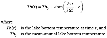
Amplitude (A) and phase (c) are estimated by means of a four‑parameter sine wave of the form:


     (18)


This is fitted by means of sinusoidal regression to the lake bottom temperature (fig. 7), based on the average of the temperatures measured 1 m above the lake bottom at water‑quality stations MDN, EPT, SET, and MDT (fig. 1; T.M. Wood, U.S. Geological Survey, unpub. data). Janssen (2005) found no statistical difference between daily lake bottom temperatures and corresponding Link River temperatures. Therefore, if no records were available from any of the water-quality stations for a day or period of days, daily mean temperatures at the Link River were used.


Changes in Energy Stored in the Lake


Changes in energy stored in the Upper Klamath Lake were estimated using the same well-mixed lake assumption that Janssen (2005) used for his study. This assumption is based on the findings of Wood and others (2006), who demonstrated that Upper Klamath Lake does not develop a strong thermocline due to its shallow depth. When thermal stability does develop, it typically disappears in less than a day (Wood and others, 2006). The following equation is used to estimate the changes in stored energy:


     (19)


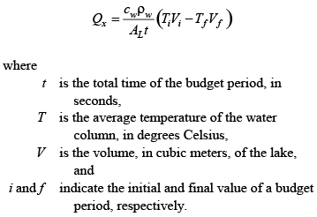
Temperature data collected at the five temperature stations on the lake (fig. 1) 1 m below the water surface and 1 m above the lake bottom were used to calculate an average water column temperature at that location. Average water column temperatures for a particular day were then averaged to estimate the mean temperature of the lake. Lake stage data from USGS gage 11507001 and storage volume, interpolated to nearest 0.01 ft (fig. 1), were used for calculations in equation 19. Dead storage of 2.61×10⁸ m³ (211,300 acre-ft; from the station description for the above referenced gage) was added to the active storage term to yield total lake volume.


Bowen Ratio


The Bowen ratio (β in the denominator of equation 11) is the ratio of sensible heat to latent heat. It is calculated (Bowen, 1926; Sturrock and others, 1992) as:


     (20)


The psychometric constant is a function of the specific heat of air c_a [1.00416 J kg^-1 °C], atmospheric pressure P [kPa] and the latent heat of vaporization λ_v (Janssen, 2005; Dingman, 2002):


     (21)


The latent heat of vaporization [J kg^-1] is a function of surface temperature and can be approximated by (Janssen, 2005; Dingman, 2002):


     (22)


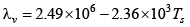
Atmospheric pressure was estimated by (Janssen, 2005; Shuttleworth, 1993):


     (23)


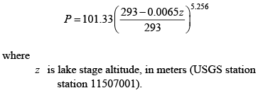
Vapor pressure of the air is estimated as:


     (24)


where RH is the relative humidity [dimensionless] and the rest of the right-hand side is the saturated vapor pressure of the air [kPa] which is a function of air temperature (Janssen, 2005; Dingman, 2002). Similarly, the vapor pressure at the water surface can be calculated as:


     (25)


As can be seen from equations 24 and 25, the vapor pressure at the surface is saturated and a function of water surface temperature.


One Bowen-ratio value was calculated for each 2-week energy budget period using air and water surface temperatures and vapor pressures (eq. 20) averaged over the period.


Determination of Reference Evapotranspiration and Crop Coefficients


Potential evapotranspiration (ET_p) is the ET that occurs from an extensive land or water surface under a given set of meteorological conditions when the surface is well supplied with water. In the most general interpretation, the concept applies to a wide range of land-surface types, from dense rainforests to bare soil. Because vegetation type, density, and vigor have a strong effect on the resulting ET_p, the need gradually arose for a more specific quantity—one that assumes a standard vegetation type and density, growing vigorously, and therefore depends only on weather conditions. Penman (1948) suggested dense grass cover as the reference vegetation, although other crops (and open water) have been suggested over the years. Computation of ET_p for a specific reference crop led to the adoption of the notation ET_r to refer to potential ET from a reference crop. During the late 20th century, the Food and Agricultural Organization (FAO) of the United Nations took the lead in standardizing the computation of ET_r, most recently through the work of Allen and others (1998), who presented the Penman-Monteith equation in a user-friendly form, for use with a 12-cm tall, dense grass reference crop. Using this methodology, ET for other well‑watered crops is computed as the product of ET_r and a crop coefficient, K_c, which varies based on growth stage of the crop:


     (26)


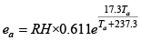
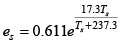
Subsequently, the American Society of Civil Engineers modified the FAO equation to also accommodate alfalfa as a reference crop (Allen and others, 2005). The Bureau of Reclamation maintains a network of weather stations in the Pacific Northwest region states that can be used to calculate ET and crop ET using the Allen and others (2005) alfalfa (tall crop) equation. Daily values of ET and crop ET are posted on the Bureau of Reclamation Web site (http://www.usbr.gov/pn/agrimet/h2ouse.html) in near real time, for use by irrigators and others.


In the current study, we divide measured values of ET from the two wetland sites by posted values of tall crop ET_r calculated from nearby weather station data to compute daily and biweekly values of K_c. Daily values of ET_r are obtained from the Agency Lake (AGKO) weather station, located about 7.1 km northeast of the bulrush site. When daily values of ET_r are equal to 0, K_c is infinite, and we arbitrarily set K_c to a value of 6. Daily values of ET and ET_r are aggregated into biweekly values to compute biweekly values of K_c. To investigate relations between K_c and precipitation, daily values of precipitation were retrieved from the Klamath Falls (KFLO) weather station, located about 44 km southeast of the bulrush site, in Klamath Falls, Oregon. This station deploys a weighing precipitation gage, which measures snowfall more reliably than the unheated tipping bucket gage at the (closer) AGKO station. Growing-season ET data from alfalfa and pasture also were retrieved from the KFLO station for comparison with measured wetland ET. These ET values were not available from the AGKO station Web site.


First posted March 4, 2013