Scientific Investigations Report 2014–5054
Groundwater-Management StrategiesManaging the limited water resources of the upper Klamath Basin is a multi-faceted problem where the consumptive uses of agriculture and instream needs of aquatic wildlife must be balanced. In 2001, actions intended to protect habitat for endangered fishes resulted in the curtailment of surface-water deliveries to the Project. In the years since, Endangered Species Act biological opinions have required the Bureau of Reclamation (Reclamation) to maintain specified levels in Upper Klamath Lake to protect habitat for Lost River and shortnose suckers while simultaneously providing flows in the Klamath River downstream of Iron Gate Dam to maintain habitat for coho salmon. This shift in water-management priorities resulted in substantial reductions in surface-water diversions to the Project in 2001 and 2010, and increases the likelihood of Project water shortages in the future. In response to changing water-management priorities, stakeholders in the basin developed the KBRA, a framework for water-resources management designed to restore aquatic habitat and provide reliable water supplies for irrigation (Klamath Basin Restoration Agreement, 2010). Although the KBRA provides for predictable surface-water diversions to the Project, those water supplies will be diminished in dry years, with irrigation-diversion deficits as much as about 100,000 acre-ft in the driest years. Surface water will not be able to meet Project irrigation demands in every year and groundwater is a potential alternative irrigation supply (Klamath Basin Restoration Agreement, 2010). Groundwater Use in the Upper Klamath BasinGroundwater use in the upper Klamath Basin is primarily for agriculture and public supply. Prior to 2001, the estimated groundwater withdrawals in the basin totaled about 160,000 acre-ft, with about 10,000 acre-ft pumped for public supply and about 150,000 acre-ft pumped for irrigation (Gannett and others, 2007). Irrigation withdrawals in the area of the Project totaled about 29,000 acre-ft or 19 percent of the total irrigation withdrawals in the basin. Since 2001, groundwater use in the upper Klamath Basin has increased considerably, mostly due to programs funded by Reclamation and KWAPA and designed to supplement the reduced surface-water supplies for the Project. The volumes of groundwater purchased by these programs are summarized in figure 2. During 2001–07, Reclamation’s Groundwater Acquisition and Pilot Water Bank programs annually pumped as much as 66,000 acre-ft to supplement the reduced surface-water diversions to the Project. This represents a maximum of 45 percent increase in basin-wide irrigation withdrawals when compared to pre-2001 pumping amounts. In 2010, Project supplemental groundwater pumping was funded by the KWAPA Water Users Mitigation Program and totaled about 101,000 acre-ft, a 67 percent increase in pre-2001 irrigation withdrawals, and roughly a four-fold increase in Project-area irrigation pumping (MBK Engineers and others, 2012a; Gall, 2011; Klamath Water Users Association, 2011). Pumping amounts shown in figure 2 represent only the amounts purchased by Reclamation and KWAPA. The total annual amounts of groundwater pumped from 2001 to 2004 to supplement Project water supplies were as much as 33,000 acre-ft higher than the amounts shown in figure 2 (McFarland and others, 2005; Gannett and others, 2007). Increased supplemental pumping for the Project during 2001–07 resulted in water-level declines of 10–15 ft over much of the Project, and hydrographs indicate water levels reached a new equilibrium with the regional groundwater system. The sharp increase in pumping in 2010, however, caused some of the largest seasonal water-level declines and lowest water levels on record, with persistent declines of 3–7 ft in some areas compared to pre-2010 groundwater levels (Gall, 2011). The effects of Project groundwater pumping are not limited to Project water users. The effects can potentially extend off-Project to surface-water features and off-Project irrigation, domestic, and municipal wells. In 2010 and 2011, KWAPA funded the Domestic and Municipal Well Mitigation Program to improve domestic and municipal supply wells adversely affected by on-Project pumping. Financial assistance was provided to well owners for the purpose of lowering pumps, deepening existing wells, and drilling new wells (Gall, 2011; Klamath Water Users Association, 2011). Hypothetical Groundwater Demand under the Klamath Basin Restoration AgreementWater use by the Project varies primarily as a function of climate, with increased irrigation demand in dry years. For this study, alternative groundwater-management strategies were simulated for 1970–2004, a 35-year management period that includes multiple wet and dry periods. The groundwater demand of the Project was defined as the difference between the demand for irrigation and the amount of surface water available for diversion to the Project. One method for estimating irrigation demand is to define the demand based on historical irrigation diversions. Prior to 2001, annual irrigation diversions from Upper Klamath Lake ranged from about 310,000 to about 430,000 acre-ft, with the highest diversions occurring during the extended drought period from 1987 to 1994 (McFarland and others, 2005; MBK Engineers and others, 2012b). Since 2001, however, Endangered Species Act restrictions have limited surface-water diversions in dry years. As a result, surface-water deliveries to the Project in 2001, 2003, and 2004 did not represent actual Project irrigation demand. Moreover, historical irrigation diversions may not reflect changes to Project operations, such as changes to cropping patterns and irrigation practices. An alternative method for estimating irrigation demand during 1970–2004 is based on Reclamation’s Klamath-Project simulation model, which estimates irrigation demand within the Project based on present-day cropping patterns, irrigation needs, and historical hydrologic conditions (MBK Engineers and others, 2012b). The approach taken in this study was to estimate the Project annual irrigation demand for each year during 1970–2004 as the larger of the historical irrigation diversion and the simulated irrigation demand. This approach also was used by KWAPA to develop the on-Project Plan, a water-use plan for the Project that is an integral component of the KBRA (Klamath Basin Restoration Agreement, 2010, section 15). In contrast to irrigation demand, the diversions allowed under the KBRA will be smallest during dry years when inflows to Upper Klamath Lake tend to be smaller than average. The diversions allowed under the KBRA Phase-1 allotment schedule are calculated as a function of projected inflows to Upper Klamath Lake during the April–October irrigation season and vary from 330,000 acre-ft in low-inflow years to 385,000 acre-ft in high-inflow years (Klamath Basin Restoration Agreement, 2010, appendix E-1). This relation of increasing Project irrigation demand with decreasing KBRA surface-water allotment creates a scenario in which the highest groundwater demand is expected in the driest years. This relation is shown in figure 3A, which shows the estimated irrigation demand with the hypothetical diversions that would be allowed under the KBRA. The differences between surface-water demands and the diversion amounts allowed under the KBRA define the hypothetical groundwater demand function that is included as constraints in the groundwater-management model. The hypothetical Project groundwater demand is shown in figure 3B and ranges from zero for years in which the calculated KBRA surface-water allotment equals or exceeds the predicted irrigation demand to about 102,000 acre-ft in the drought year of 1991. The 35-year groundwater-demand schedule has 22 years with non-zero groundwater demand. Of those 22 years, 6 years have demands less than 20,000 acre-ft, 8 years have demands of 20,000–60,000 acre-ft, and 8 years have groundwater demands that exceed 60,000 acre-ft (fig. 3B). The extended drought period from 1987 to 1994 includes 6 of the 8 years with groundwater demand greater than 60,000 acre-ft. The groundwater demand schedule shown in figure 3B assumes that irrigation-demand deficits under the Klamath Basin Restoration Agreement will be met, to the extent possible, using groundwater. The KBRA proposes additional measures to improve water supplies and reduce irrigation demand, such as demand management, efficiency measures, new surface-water storage, and land and water acquisitions. Since 2001, however, Reclamation and KWAPA have relied primarily on a combination of groundwater pumping to supplement surface-water supplies and demand management (in the form of temporary land idling) to reduce irrigation demand. In 2010, KWAPA purchased approximately 101,000 acre-ft of groundwater at an average cost of about 25 dollars per acre-foot. At the same time, KWAPA accepted bids to idle approximately 36,000 acres of farmland within the Project at an estimated cost of about 85 dollars per acre-foot of reduced irrigation-water demand (Klamath Water Users Association, 2011). The cost difference suggests that groundwater substitution will be an important means to bridge the periods of reduced surface-water diversions foreseen under the KBRA. Groundwater is expected to be an important supplemental water supply for Project irrigators. If the marked increase in pumping since 2001 is sustained, a new state of dynamic equilibrium eventually will be reached, with unknown effects to groundwater and surface-water resources throughout the basin. As a result, groundwater users and resource-management agencies in the upper Klamath Basin need methods to identify groundwater-management strategies that meet the double goals of increased groundwater production and resource protection. Simulation-Optimization ModelGroundwater-development alternatives for the upper Klamath Basin were evaluated with the aid of a coupled simulation and optimization groundwater-management model. The simulation model described in Gannett and others (2012) was used to estimate the spatial and temporal distribution of pumping related drawdowns; the effects of pumping on streams, springs, and lakes critical to aquatic wildlife; and the effects on agricultural drains that provide irrigation water to farmers in the Project and also are a source of water for national wildlife refuges within the Project boundaries. The simulation model was coupled with an optimization algorithm to form a groundwater-management model that was used to identify solutions for improving groundwater use in the Project. The groundwater-management model provides a tool for efficiently processing and ranking groundwater-management alternatives and identifying solutions that best meet the goals of water users and resource-management agencies. Literature reviews of simulation-optimization research are available in Gorelick (1983), Yeh (1992), Wagner (1995), and Ahlfeld and Mulligan (2000). Example applications of the simulation-optimization approach that include groundwater–surface-water interactions include Barlow and Dickerman (2001), DeSimone and others (2002), Granato and Barlow (2004), and Gannett and others (2012). A groundwater-management model for the upper Klamath Basin was developed and tested in a previous study (Gannett and others, 2012). In that study, the goal was to determine the maximum annual pumping amount that could be sustained over a 20-year period; the optimal groundwater-pumping strategies were identified using a dynamic steady-state groundwater-simulation model that was based on average historical climate conditions. The simulation model used in that study did not include off-Project supplemental pumping and the simulation-optimization model did not explicitly account for the Project groundwater demand as foreseen under the KBRA. This report describes the development and application of an enhanced groundwater-management model that incorporates variable hydrologic conditions from the recent historical record. The simulation model used in this study also incorporates time-varying background supplemental pumping that accounts for increased groundwater withdrawal by off-Project irrigators during drought periods. Finally, a groundwater-demand function (fig. 3B) derived from the KBRA surface-water-allotment formula is incorporated in the groundwater-management model to account for the Project time-varying groundwater needs. Potential Adverse Effects of Groundwater DevelopmentThe fundamental goal of the enhanced upper Klamath Basin groundwater-management model is to determine the spatial and temporal distribution of pumping that, to the extent possible, meets the hypothetical Project groundwater demand (fig. 3B) while avoiding adverse effects to groundwater and surface-water resources. These effects include the link between groundwater pumping and groundwater discharge that supports aquatic habitat, the effect of increased pumping on water levels throughout the Project and adjacent areas, and the effect of groundwater withdrawal on irrigation return flows that are essential to Project operations. Groundwater discharge provides a substantial proportion of streamflow in the upper Klamath Basin and is particularly important during the April–October irrigation season when precipitation is low and there are competing agriculture and ecological water demands. The KBRA provides measures for defining and limiting the adverse effects of groundwater pumping on streams and springs in the basin. The KBRA defines adverse effects as a 6 percent or greater reduction in groundwater discharge to springs associated with Upper Klamath Lake, the Wood River and its tributaries, Spring Creek and the lower Williamson River, and the Klamath River and its tributaries (fig. 1). The KBRA further defines the measure of pumping related effects on surface-water resources to include only the effects resulting from groundwater use within the Project. That is, all off-Project pumping in the basin is considered part of the baseline conditions against which the effects of on-Project pumping will be measured (Klamath Basin Restoration Agreement, 2010, section 15). The groundwater-management model also must consider the effects of groundwater development on existing groundwater users. The OWRD controls new groundwater appropriations and can regulate pumping to protect senior water-right holders (Oregon Water Resources Department, 2011). Since 2000, OWRD has been applying water-level-decline limits to new groundwater-right permits in the upper Klamath Basin. The permit conditions constrain drawdown at various time scales. Seasonal drawdown constraints limit the water-level declines that develop during the irrigation season, year-to-year drawdown constraints limit the drawdown remaining at the beginning of the irrigation season because of the previous year withdrawal, and long-term drawdown constraints limit the water-level declines that accumulate over a 10-year period. Groundwater development currently (2013) is not regulated in the California part of the upper Klamath Basin; therefore, initial applications of the groundwater-management model apply OWRD drawdown limits in the Oregon and California parts of the model. Sensitivity analysis is used to test the effect of alternative drawdown limits. Finally, the groundwater-management model must evaluate the reductions in groundwater discharge to the Project drain system caused by groundwater pumping. Studies of groundwater use within irrigated agricultural areas in the western United States have shown that substantial amounts of pumped groundwater can originate as irrigation water that is captured by pumping wells (Reilly and others, 2008). In the Project, irrigation return flows are recirculated through the drain system and can be a significant water supply for downslope irrigators. Irrigation return flows also are used to maintain permanent and seasonal wetlands in the Tule Lake and Lower Klamath National Wildlife Refuges (Burt and Freeman, 2003; Risley and Gannett, 2006). Any groundwater discharge diverted from the drain system by pumping will reduce the amount of water available for irrigation and delivery to the refuges. The groundwater-management model is designed to evaluate and limit the effects of groundwater pumping on the Project drain system. The analyses described in this report were limited by the lack of information available to define the Project demand for irrigation return flows. Therefore, the groundwater-management model was solved for a varied set of drain flow-reduction limits to provide information on the sensitivity of management-model results. Formulation and Solution of the Groundwater-Management Model, 1970–2004The groundwater-simulation model described in Gannett and others (2012) was coupled with an optimization algorithm to identify solutions that improve groundwater production for the Klamath Project. The manageable components of the optimization model are the time-varying pumping rates at 117 wells distributed throughout the Project (fig. 4A). Constraint equations set limits on drawdowns at various time scales, reductions in groundwater discharge that support aquatic habitat, reductions in groundwater discharge to the Project drain system, annual groundwater-pumping goals, and the maximum pumping rate at each well. The optimization problem is formulated as a linear programming problem: Maximize subject to:
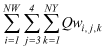
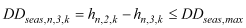
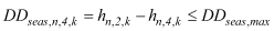
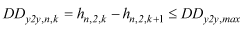
where: Qwi,j,k is the pumping rate at managed well i in quarter j of water year k; NY is the number of years in the management horizon and equals 35; NW is the number of decision wells and equals 35 (note that well aggregation is used to reduce the number of decision variables); i is the well number; j is the water year quarter, 1–4, with water year quarters 3 and 4 comprising the April to October irrigation season; k is the year, with k=1 corresponding to water year 1970; DDseas,n,3,k is the seasonal drawdown at constraint location n at the end of quarter 3 (mid-point of irrigation season) in water year k; hn,2,k is the head at control location n at the end of quarter 2 (beginning of irrigation season) in water year k; hn,3,k is the head at control location n at the end of quarter 3 (mid-point of irrigation season) in water year k; DDseas,max is the upper bound on seasonal drawdown; DDseas,n,4,k is the seasonal drawdown at constraint location n at the end of quarter 4 (end of irrigation season) in water year k; hn,4,k is the head at control location n at the end of quarter 4 (end of irrigation season) in water year k; DDy2y,n,k is the year-to-year drawdown at constraint location n in water year k; DDy2y,max is the upper bound on year-to-year drawdown; DD10yr,n,k is the decadal drawdown at constraint location n in water year k; DD10yr,max is the upper bound on decadal drawdown; hn,min is the lower bound on head at control location n; QSRn,j,k is the reduction in groundwater discharge to stream reach n in quarter j of water year k; qsrn,j,k,base is the groundwater discharge to stream reach n in quarter j of water year k for baseline conditions with no Project pumping; qsrn,j,k,man is the groundwater discharge to stream reach n in quarter j of water year k for managed conditions with optimized Project pumping; QSRn,j,k,max is the maximum allowable reduction in groundwater discharge to stream reach n in quarter j of water year k, QLRj,k is the reduction in groundwater discharge to Upper Klamath Lake in quarter j of water year k; qlrj,k,base is the groundwater discharge to Upper Klamath Lake in quarter j of water year k for baseline conditions with no Project pumping; qlrn,j,k,man is the groundwater discharge to Upper Klamath Lake in quarter j of water year k for managed conditions with optimized Project pumping; QLRj,k,max is the maximum allowable reduction in groundwater discharge to Upper Klamath Lake in quarter j of water year k, QDRj,k is the reduction in groundwater discharge to Project drains in quarter j of water year k; qdrj,k,base is the groundwater discharge to Project drains in quarter j of water year k for baseline conditions with no Project pumping; qdrj,k,man is the groundwater discharge to Project drains in quarter j of water year k for managed conditions with optimized Project pumping; QDRj,k,max is the maximum allowable reduction in groundwater discharge to Project drains in quarter j of water year k; QDEMk is the groundwater demand for water year k, defined as the quarterly pumping rates that are needed to meet the annual groundwater demand shown in figure 3B. The values of QDEMk are determined by dividing the annual groundwater demand (in acre-ft) by 181; nsr is the number of stream reaches with groundwater discharge constraints and equals 34. Qwi,max is the maximum withdrawal rate for decision well i; and ndd is the number of drawdown constraint locations and equals 337.
The objective function (equation 1) sums the quarterly pumping at each managed well during water-year (the 12-month period from October 1, for any given year, through September 30 of the following year) quarters 3 and 4, which comprise the irrigation season, for each year of the 35-year management period. The managed wells used in the optimization model are shown in figure 4A and represent the wells used in Reclamation’s Groundwater Acquisition and Pilot Water Bank programs and KWAPA’s Water Users Mitigation Program. The optimization model calculates the pumping rates for the 117 managed wells shown in figure 4A; all other wells in the model are considered to be background stresses that contribute to the total stress acting on the groundwater system, but do not change from one simulation to the next. In this study, aggregated pumping rates are used to define the decision variables of the groundwater-management model. Each decision variable, Qwi,j,k, was defined as a subset of the managed wells shown in figure 4A and represents the aggregated quarterly withdrawal from a localized area of the Project. For each aggregated decision variable, the optimization model determines a single value that is distributed among the wells comprising that decision variable and that is apportioned according to the pumping capacity for each well. The analyses described in this report include 35 aggregated decision wells formed by the 117 individual wells shown in figure 4A; the number of individual wells in each aggregated well group ranges from one to six, with an average of about three wells per group. The groundwater-management model calculates 3rd and 4th quarter pumping rates (in units of cubic feet per second) for the 35 aggregated decision wells in each of the 22 years with non-zero groundwater demand, for 1,540 decision variables. Multiplying the quarterly groundwater-pumping rates by 181 defines the volume of groundwater pumped in units of acre-feet. Pumping volumes are used to describe the results of the groundwater-management model in the remainder of the report. Well aggregation reduces the number of decision variables in the optimization model, which reduces the computational effort required to solve each optimization problem. The well-aggregation method, however, also reduces the flexibility of the management solution by limiting the manner in which well rates within an aggregated well group can vary relative to each other. The effect of well aggregation is a suboptimal solution when compared to the solution obtained without aggregation. The amount by which the well-aggregation method underestimates the optimal pumping can be determined only by solving the non-aggregated optimization model, which will be different for every formulation of the optimization problem. An example of simulation-optimization modeling with well aggregation is available in Barlow and others (1996). Equations 2–11 define the constraints of the optimization model; that is, the measures used to define the success or failure of alternative groundwater-management plans. Groundwater withdrawal can have short- and long-term effects on water levels. The optimization model includes constraints on drawdown at 337 control locations shown in figure 4B. Drawdown controls were applied at the 117 model cells that contain managed wells along with 220 model cells that contain off-Project pumping wells within 6 mi (12 model cells) of a managed well. Four types of drawdown constraints were applied at each control location: (1) seasonal drawdown constraints (equations 2 and 3) were defined to limit the lowering of water levels during the irrigation season, (2) year-to-year drawdown constraints (equation 4) were defined to limit the residual drawdown remaining at the beginning of the irrigation season because of the previous year withdrawal, (3) a drawdown constraint (equation 5) was included to limit the long-term drawdown simulated over a decade, and (4) a constraint was included to impose a maximum drawdown by defining the minimum allowable head at each location (equation 6). The seasonal, year-to-year, and decadal drawdown limits, DDseas,max, DDy2y,max, and DD10yr,max, were set to 25, 3, and 25 ft, respectively, in the base-case optimization model, as required by Oregon water law (Oregon Water Resources Department, 2011). At each drawdown constraint location, the minimum allowable head, hn,min, was set to 25 ft below the simulated 2001 pre-irrigation-season water level. A sensitivity analysis was done to assess the effect of varying the seasonal, year-to-year, and 10-year drawdown limits. The groundwater-management model included two seasonal drawdown constraints at each drawdown-control site in each year of the model, for a total of 23,590 seasonal drawdown constraints; 34 year-to-year drawdown constraints at each control site, for a total of 11,458 year-to-year drawdown constraints; 25 10-year drawdown constraints at each control site, for a total of 8,425 10-year drawdown constraints; and 35 minimum head constraints at each control site, for a total of 11,795 minimum head constraints. Year-to-year and 10-year drawdown constraints do not extend beyond 2004; therefore, effects of pumping that occurred after 2004 were not evaluated in the groundwater-management model. Groundwater withdrawal is accompanied by declines in water levels that interact with surface water at various temporal and spatial scales, potentially causing reductions in groundwater discharge to streams, lakes, and drains. Constraints on the reduced groundwater discharge to streams (equation 7) required the reduction to be less than or equal to a specified maximum at the end of each of the 140 simulated water-year quarters for 34 stream reaches (fig. 4B), for a total of 4,760 groundwater discharge constraints for streams. A similar set of quarterly discharge constraints (equation 8) is defined to limit reductions in groundwater discharge to Upper Klamath Lake, for a total of 140 groundwater discharge constraints for Upper Klamath Lake. The limits to the constraints controlling groundwater discharge to streams and Upper Klamath Lake, QSRn,j,k,max and QLRj,k,max, were set to 6 percent of the simulated baseline groundwater discharge, as specified in the KBRA, and were fixed in all model runs. Additional constraints were defined to limit the reduction in groundwater discharge to the Project drain system (equation 9), for a total of 140 groundwater-discharge constraints for drains. The limit on the reduction in groundwater discharge to drains, QDRj,k,max, was initially set to 20 percent of the simulated baseline groundwater discharge. The effect of the drain-discharge limit in equation 9 was tested using sensitivity analysis. Demand constraints (equation 10) were included to limit total pumping in each year with supplemental groundwater demand, for a total of 22 groundwater-demand constraints. Constraint limits, QDEMk, were defined using the hypothetical groundwater demand shown in figure 3B. Finally, capacity constraints (equation 11) define the maximum withdrawal rate for each aggregated decision well, Qwi,max. Capacity limits were defined for each well included in an aggregated well group and summed to define the constraint limit for that aggregated decision variable. Pumping capacities at individual wells were determined from water-well reports obtained from the states or pump information obtained from the KWAPA. The groundwater-management model includes 1,540 capacity constraints, one for each of the decision variables. The coupled simulation and optimization groundwater-management model represented by equations 1–11 includes 1,540 decision variables and 61,870 constraints. The groundwater management model was solved using the method of sequential linear programming (Ahlfeld and Mulligan, 2000), which accounts for the nonlinearities associated with head-dependent boundaries used to model streams, lakes, drains, and evapotranspiration surfaces in the upper Klamath Basin groundwater-simulation model. Sequential linear programming solves a series of linear-programming problems, each formulated using the response matrix technique (Gorelick and others, 1993; Ahlfeld and Mulligan, 2000). The optimization model was solved in each iteration of the sequential linear programming method using the optimization software package, LINDO® (LINDO Systems Inc., 2005). The sequential solution process is continued until the optimization solution reaches convergence. The primary convergence criterion used in this study is based on the objective function value (equation 1), and requires that the change in this value from iteration l to iteration l+1 be less than 0.1 percent. A discussion of the response-matrix approach and sequential linear programming, and their application to the upper Klamath Basin groundwater model is available in Gannett and others (2012). Detailed developments of the response-matrix technique can be found in Gorelick and others (1993) and Ahlfeld and Mulligan (2000). Example applications of the sequential linear programming approach are available in Danskin and Gorelick (1985), Danskin and Freckleton (1989), Nishikawa (1998), Reichard and others (2003), Ahlfeld and Baro-Montes (2008), and Gannett and others (2012). Variations of Groundwater Levels Under Background ConditionsGroundwater systems are dynamic, with groundwater recharge, groundwater discharge, and groundwater levels varying in response to external stresses. The largest external stresses affecting groundwater in the upper Klamath Basin are drought cycles and groundwater pumping (Gannett and others, 2007, 2012). Drought cycles cause variations in groundwater recharge, which are manifest as fluctuations in water levels and groundwater discharge to springs and streams. Pumping also affects water levels and groundwater discharge, with the greatest effects observed near the pumping stress. The groundwater-management model developed for this study limits short- and long-term variations in water levels through the drawdown constraints defined by equations 2–6. Unlike the groundwater-discharge constraints (equations 7–9), which limit the relative changes in groundwater discharge caused by on-Project pumping, the drawdown constraints limit the absolute changes in water levels and do not distinguish between changes caused by on-Project pumping and changes caused by background pumping or climate. Because of this, drawdown constraints can be violated (that is, the constraint is not met) solely in response to background pumping conditions and climate cycles. Violations under background conditions can occur in areas where (1) actual conditions are close to, or actually exceed, drawdown limits; (2) the simulated response to an external stress is larger than the true response; or (3) there are errors in the estimates of background pumping. A pre-optimization groundwater-modeling analysis was done to identify the extent of drawdown-constraint violations caused by background pumping and climate. The simulation model was run with the on-Project pumping set to zero to identify the locations and times at which drawdown constraints are violated under background conditions. The groundwater-management model includes 337 drawdown-control sites with 55,268 drawdown constraints; the pre-optimization groundwater-modeling analysis identified 48 locations with 1,050 background constraint violations. The locations of the drawdown constraints violated under background conditions are shown in figure 4B. Most drawdown constraints are located on the margins of the managed area. Twenty-five constraint locations with background violations are located along the western margin among the drawdown-control locations north of the Klamath River and in the western part of the Lower Klamath Lake region; 15 constraint locations are in the upper Lost River region. Of the remaining eight locations, two are in the Klamath Valley region and six are in the northern Tule Lake region. Five of the 48 locations with background violations are at drawdown-control sites that are co-located with managed wells. Of the 1,050 violated drawdown limits, 764 are seasonal drawdown-constraint violations, 245 are year-to-year drawdown-constraint violations, and 41 are 10-year drawdown-constraint violations. There are no violations of the minimum-head constraint (equation 6). The groundwater-management model was modified to account for these background constraint violations and allow solution of the optimization model defined by equations 1–11. For each of the 1,050 location and time couplets with a drawdown-constraint violation, the drawdown limit was modified. The drawdown limit (DDseas,max, DDy2y,max, or DD10yr,max) was revised to be the simulated background groundwater-elevation change plus an exceedance tolerance of 0.2 ft. The exceedance tolerance was constant across all 48 sites with background violations and all drawdown-constraint types. Alternative values of the exceedance tolerance, ranging up to 0.5 ft, also were tested, with no significant changes in the results of the groundwater-management model. Evaluation of Selected AlternativesBase-Case AnalysisThe base-case optimization model uses the groundwater-management model described in this report. The goal of the base-case analysis is to determine the ability of the groundwater system to reduce or eliminate annual surface-water deficits of the Project foreseen under the KBRA, and to identify the spatial and temporal pattern of pumping that best meets that goal. Subsequent analyses will explore the sensitivity to several factors—restrictiveness of drawdown constraints, drain-discharge constraint limits, additional pumping capacity, and targeted reduction of background pumping. Table 1 summarizes the alternative analyses described in this report. The results of the base-case optimization model are summarized in figures 5–7 and table 2. The optimization model yields individual rates for each decision well shown in figure 4A; however, it is the spatial and temporal patterns of pumping that are useful for practical implementation of a groundwater-management strategy. The withdrawals calculated by the optimization model indicate the following:
The groundwater-management model includes constraints to control the effects to groundwater and surface-water resources within and outside the Project. With the spatial and temporal patterns of withdrawal summarized in table 2 and figure 5, the binding constraints (those constraints calculated to be at their limits) were associated with seasonal, year-to-year, and 10-year drawdowns (equations 2–5). Of the 677 binding constraints that occurred during the entire 35-year management period, 576 are associated with seasonal drawdowns (264 are binding in the 3rd quarter and 312 are binding in the 4th quarter), 98 are associated with year-to-year drawdowns, and 3 are associated with 10-year drawdowns. The locations and the frequency of occurrence of the binding drawdown constraints are summarized in figure 7. Binding seasonal drawdown constraints that occur in the 3rd quarter are at 30 locations shown in figure 7A, with all 30 binding constraint sites co-located with managed wells. The wells with frequently binding constraints occur primarily in the southern Tule Lake, northern Tule Lake, and Klamath Valley regions where the highest pumping volumes occur. Similarly, for the 4th quarter seasonal drawdown constraints, 36 of the 41 binding drawdown sites are in model cells with managed wells; the locations with the highest frequency of binding constraints occurred in the Klamath Valley and northern Tule Lake regions (fig. 7B). For the year-to-year drawdown constraints, binding constraints occurred at 36 locations, with 30 co-located with managed wells; the locations of the frequently binding constraints are in the Klamath Valley, northern Tule Lake, and southern Tule Lake regions (fig. 7C). The binding 10-year drawdown constraints (not shown in figure 7) are north of the Klamath River at two background (non-managed) well sites. The binding drawdown constraints summarized in figure 7 include constraints that are violated in response to background pumping and climate cycles. The groundwater-management model includes 1,050 drawdown constraints that were modified to account for violations under background conditions (fig. 4B). Of the 677 binding drawdown constraints in the base-case analysis, 33 occurred in the set of modified constraints associated with violations under background conditions. The subset of 33 constraints (29 seasonal, 1 year-to-year, and three 10-year drawdown constraints) is located at 7 drawdown locations, of which 3 are co-located with managed wells. The spatial and temporal distribution of these 33 constraints indicates they have varying effects on the results of the groundwater-management model. Eighteen of the 33 binding constraints occur in years when the groundwater-management model calculation meets supplemental irrigation demand. The remaining 15 binding constraints occur in years with unmet groundwater demand and are co-located with 3 decision wells. Thirteen constraints are co-located with a decision well in the northern Tule Lake region that has an aggregated pumping capacity of approximately 4,100 acre-ft; pumping volumes calculated by the groundwater-management model for this decision well are less than 400 acre-ft. One constraint is co-located with a decision well in the Klamath Valley region that has an aggregated pumping capacity of approximately 6,800 acre-ft; pumping volumes calculated by the groundwater-management model for this decision well have a maximum of approximately 1,100 acre-ft. The final constraint is co-located with a decision well in the Klamath River well group that has an aggregated pumping capacity of approximately 1,900 acre-ft; pumping volumes calculated by the groundwater-management model for this decision well have a maximum of approximately 900 acre-ft. The below-capacity pumping volumes calculated for these three decision wells occur throughout the management period, including years when the drawdown constraints are not binding under background conditions. Fluctuations in groundwater levels due to background pumping and climate were observed to varying degrees at all drawdown-control sites, and constraint violations due to background conditions were expected. In the base-case groundwater-management analysis, the constraint violations under background conditions potentially affect maximum rates at a small number of individual wells. Because the groundwater-management model includes 117 wells distributed over a large geographic region, the effect of these violations on the overall management-model results is small. Future analyses of groundwater management in the upper Klamath Basin should consider regulatory controls that might affect groundwater development in areas where drawdown constraints are violated under background conditions. Evaluation of Sensitivity to Less Restrictive Drawdown Constraints in CaliforniaThe State of California provides three basic methods for managing groundwater resources: (1) court adjudication, (2) local government ordinances, and (3) management by local agencies under authority granted by State statutes (California Department of Water Resources, 2003). Presently (2013) these controls are not applied to groundwater development in the California part of the upper Klamath Basin. As a result, alternative values for drawdown limits in the California part of the Project may be considered in future groundwater planning. The first sensitivity analysis tests the effect of less restrictive seasonal and year-to-year drawdown constraints in the California part of the Project, as summarized in table 1. The base-case optimization model constrains seasonal drawdown (25 ft), year-to-year drawdown (3 ft), and decadal drawdown (25 ft) according to limits assigned by the OWRD. In this two-part sensitivity analysis, the drawdown limits for seasonal-drawdown constraints (equations 2 and 3) and year-to-year drawdown constraints (equation 4) are first changed to 37.5 and 4.5 ft, respectively, at all drawdown-control locations in the California part of the model (scenario DD_1 in table 1). A second formulation of the groundwater-management model changes the constraints to 50 ft for seasonal drawdown and 6 ft for year-to-year drawdown (scenario DD_2 in table 1). For both analyses, the decadal drawdown limit remains at the base-case value of 25 ft; all other aspects of the groundwater-management model also remain the same as in the base-case analysis. Applying less restrictive seasonal and year-to-year drawdown limits while maintaining the long-term drawdown limit at the base-case value of 25 ft will allow for concentrated pumping in years with greater groundwater demand while limiting the long-term effects of sustained groundwater withdrawal. The drawdown limits used in these analyses were selected for illustration purposes. Relaxing the drawdown limits allows for substantially increased pumping in years when groundwater demand was not met in the base-case analysis. Quarterly groundwater withdrawals by pumping region are given in tables 3 and 4, and the trade-off between total annual groundwater withdrawal and drawdown limits is shown in figure 8. For both scenarios with less restrictive drawdown constraints, groundwater withdrawals met demand in 1977, 1987, and 1988, which had deficits of roughly 11,000 , 15,000, and 12,000 acre-ft, respectively, in the base-case analysis. For drawdown scenario DD_2, demand also was met in 2001, which has a deficit of roughly 13,000 acre-ft in the base-case analysis. The annual withdrawals calculated by the model increased by as much as about 22,000 acre-ft when the seasonal and year-to-year drawdown limits were 37.5 and 4.5 ft, respectively, and increased by as much as about 31,000 acre-ft when the limits were increased to 50 and 6 ft. The average groundwater withdrawal in years with unmet groundwater demand was about 70,000 acre-ft in drawdown scenario DD_1 and 76,000 acre-ft in drawdown scenario DD_2 (compared to an average withdrawal of about 54,000 acre-ft in the base-case analysis). In drawdown scenario DD_1, annual groundwater withdrawals calculated by the optimization model meet groundwater demand in 17 of 22 years; in scenario DD_2, calculated withdrawals meet demand in 18 of 22 years. The effects of varying the drawdown-constraint limits occur primarily in the pumping amounts calculated for the southern Tule Lake, northern Tule Lake, and Klamath Valley well groups, which have the highest annual withdrawals in the base-case analysis. The pumping amounts calculated for these well groups display the highest sensitivity to changes in the formulation of the groundwater-management model for all scenarios tested in this study; therefore, the discussion in the remainder of the report will emphasize the changes to calculated withdrawals for these three regions that result from changes in the formulation of the groundwater-management model. The annual groundwater withdrawals for southern Tule Lake, northern Tule Lake, and Klamath Valley well groups for the base-case and less restrictive drawdown analyses are shown in figure 9. The pumping volumes shown in figure 9 are for the years with unmet groundwater demand in the base-case optimization model (fig. 5 and table 2). The largest changes in groundwater withdrawals occur in the southern Tule Lake well group (fig. 9A), which is entirely in the California part of the basin. In drawdown scenario DD_1, the calculated withdrawals from the southern Tule Lake wells reach a maximum of about 40,000 acre-ft (compare to the base-case analysis, which had a maximum withdrawal at southern Tule Lake wells of 28,000 acre-ft). In scenario DD_2, the calculated withdrawals at the southern Tule Lake wells reach a maximum of about 52,000 acre-ft. There also is an increase in the maximum annual withdrawals from the northern Tule Lake wells (fig. 9B), which provide a maximum of about 20,000 acre-feet in drawdown scenario DD_1 and 19,000 acre-ft in scenario DD_2, as compared to a maximum of 14,000 acre-ft in the base-case analysis. However, during the entire management period, the volumes pumped from the northern Tule Lake wells are reduced in some years when compared to the base-case optimization results. For example, in scenario DD_2, there are substantial reductions in groundwater withdrawals from the northern Tule Lake wells in 1977, 1987, and 1988, when compared to the base-case analysis. This occurs because the less restrictive drawdown constraints allow groundwater demand for these years to be satisfied through increased withdrawals at the southern Tule Lake wells. As a result, groundwater withdrawal at the northern Tule Lake wells can be reduced. In contrast to the base-case analysis, the drain-discharge constraint (equation 9) is binding in the scenarios DD_1 and DD_2. As a result, the increased withdrawals are accompanied in some years by reduced withdrawals from the Klamath Valley region of the model, as shown in figure 9C. This trade-off is required to balance the increased pumping from the California part of the model and the associated effects on groundwater discharge to the Project drain system. In scenario DD_1, the drain-discharge constraint becomes binding at the end of 1991 and again at the end of 1992; and in scenario DD_2, the constraint is binding in 1990, 1991, 1992, and 1994. The effects of the binding drain-discharge constraints are apparent in the annual pumping amounts for 1991 and 1992. To maintain a feasible solution while maximizing total pumping amounts across all managed wells, withdrawals from the Klamath Valley well group are reduced by as much as about 6,000 acre-ft (scenario DD_1) and 9,000 acre-ft (scenario DD_2), when compared to the base-case results. The binding drain-discharge constraints likely also affect the amounts pumped in the northern Tule Lake region; the optimized annual withdrawals for these wells are reduced in 1990, 1991, and 1992 when the drawdown constraints are changed from scenario DD_1 to scenario DD_2 (fig. 9B). The introduction of binding drain-discharge constraints is accompanied by a reduction in the number of binding drawdown constraints. In the base-case analysis, there are 677 binding drawdown constraints across the entire management period. In scenario DD_1, there are 648 binding drawdown constraints (533 seasonal, 111 year-to-year, and four 10-year) and in scenario DD_2, there are 477 binding drawdown constraints (398 seasonal, 77 year-to-year, and two 10-year). The reduction in the number of binding drawdown constraints occurs because of the reduced pumping in the northern Tule Lake and Klamath Valley regions. Compared with the base-case analysis, the proportion of binding drawdown constraints is higher in the southern Tule Lake region where the largest increases in pumping occur. The groundwater-management model described in this report maximizes total pumping across the entire network of Project wells and does not include groundwater-demand constraints for the different regions of the Project. For the analysis with less restrictive drawdown constraints, the increased pumping volumes calculated by the groundwater-management model occur in the downslope region of the Project, primarily in the southern Tule Lake well group. Because of the Project infrastructure, groundwater withdrawals from the southern Tule Lake wells can be applied only to irrigate lands in the southern Tule Lake or Lower Klamath Lake regions, or delivered to wetlands in the Lower Klamath National Wildlife Refuge. Future analyses of groundwater management for the Project should consider additional constraints to align the geographic distribution of groundwater pumping with water demand. Evaluation of Sensitivity to More Restrictive Drawdown ConstraintsAn alternative to the evaluation of less restrictive seasonal and year-to-year drawdown limits in the California part of the model could include evaluation of the spatial and temporal distribution of pumping under more restrictive limitations on drawdown. The second sensitivity analysis tests the effect of imposing more restrictive seasonal, year-to-year, and 10-year drawdown limits throughout the Project and adjacent areas, as summarized in table 1. The base-case optimization model constrains seasonal, year-to-year, and 10-year drawdowns to be no greater than 25, 3, and 25 ft, respectively. In this sensitivity analysis, the drawdown limits for seasonal, year-to-year, and 10-year drawdowns are reduced to 20, 2, and 20 ft, respectively, at all drawdown-control sites (this scenario is denoted DD_3 in table 1). As in the analysis of less restrictive drawdown limits in the California part of the model, the revised drawdown limits were selected for illustration purposes. The groundwater-management model calculated substantial reductions in groundwater withdrawals for the case with more restrictive drawdown limits. Quarterly groundwater withdrawals by pumping region are summarized in table 5 and annual groundwater withdrawals are shown in figure 10. In the base-case analysis, maximum annual withdrawal is about 60,000 acre-ft and the average annual withdrawal in years with unmet groundwater demand is about 54,000 acre-ft. With the more restrictive drawdown limits, the maximum annual withdrawal is about 43,000 acre-ft and the average withdrawal in years with unmet demand is about 33,000 acre-ft. In addition to the overall reduction in annual withdrawals, there also is a reduction in the number of years in which groundwater demand is satisfied. In the base-case analysis, groundwater demand is met in 14 of the 22 years with non-zero demand and the maximum unmet groundwater demand is about 45,000 acre-ft; with more restrictive drawdown constraints, groundwater demand is met in only 9 of 22 years and the maximum amount of unmet groundwater demand is about 69,000 acre-ft. Substantial reductions in groundwater withdrawal occur in the southern Tule Lake, northern Tule Lake, and Klamath Valley well groups when the drawdown-constraint limits are more restrictive. The annual pumping volumes for these well groups for the base-case and drawdown scenario DD_3 are shown in figure 11. The pumping volumes shown in figure 11 are for the years with unmet groundwater demand in the base-case analysis (fig. 5 and table 2). The effect of more restrictive drawdown limits is reduced annual pumping in all years (fig. 11). The reduction in annual withdrawal from the southern Tule Lake wells is as much as about 13,000 acre-ft (fig. 11A), the reduction in annual withdrawal from the northern Tule Lake wells is as much as about 9,000 acre-ft (fig. 11B), and the reduction in annual withdrawal from the Klamath Valley wells is as much as about 11,000 acre-ft (fig. 11C). The application of more restrictive drawdown limits is accompanied by a change in the number of binding drawdown constraints in the groundwater-management model. In the base-case analysis, there are 677 binding drawdown constraints across the entire management period. When the drawdown limits are reduced, the number of binding drawdown constraints increases to 738, with the increase associated primarily with 4th quarter seasonal drawdown constraints and year-to-year drawdown constraints. Evaluation of Sensitivity to Changes in the Drain Constraint LimitThe third sensitivity analysis tests the effect of changing the limit on reductions in groundwater discharge to the Project system of drains. Studies by Burt and Freeman (2003) and Risley and Gannett (2006) highlighted the importance of irrigation return flows to the operation of the Project, which has about 700 mi of drains that collect return flows that can then be recycled for irrigation in downslope areas of the Project or routed to wetlands in the Lower Klamath and Tule Lake National Wildlife Refuges. Irrigation return flows are a substantial, although not quantified, water supply for some downslope irrigation districts and the re-use of return flows significantly increases the Project-wide irrigation efficiency (Burt and Freeman, 2003). The Project infrastructure does not provide detailed measurements of the spatial and temporal patterns of drain discharge; therefore, data are not available to accurately characterize the demand for irrigation return flows or the allowable reduction in drain discharge caused by increased supplemental groundwater pumping. As a result, the limit of the drain-discharge constraint (equation 9), QDRj,k,max, is uncertain and the evaluation of the effect of different constraint values on the optimal solution is important because changing QDRj,k,max could substantially change the amount and distribution of pumping. A sensitivity analysis was performed to test the effect of changing the limit on reductions in groundwater discharge to the Project system of drains, as summarized in table 1. In the base-case analysis, the allowable reduction in groundwater discharge to drains, QDRj,k,max, was set to 20 percent of the baseline discharge and was not limiting. Because the drains constraint was not limiting, applying a less restrictive drain constraint (that is, increasing the value of QDRj,k,maxin equation 9) will not affect the solution of the groundwater-management model; however, making the constraint more restrictive (that is, reducing the value of QDRj,k,max in equation 9) will eventually cause a reduction in total pumping. The goal of this two-part sensitivity analysis was to determine the change in pumping volume and distribution associated with a more restrictive drains-discharge constraint. In the first analysis, the drains-discharge constraint limit, QDRj,k,max, was reduced to 10 percent (this scenario is denoted Drain_10 in table 1). A second analysis further reduced the constraint limit to 5 percent (this scenario is denoted Drain_05 in table 1). The groundwater-management model calculated substantial reductions in groundwater withdrawals for both analyses. Quarterly groundwater withdrawals by pumping region are summarized in tables 6 and 7, and the trade-off between total annual groundwater pumping and allowable drainflow reduction is summarized in figures 12 and 13. In the base-case analysis, with QDRj,k,max defined based on an allowable reduction of 20 percent, the maximum annual withdrawal is about 60,000 acre-ft and the average annual withdrawal during years with unmet groundwater demand is about 54,000 acre-ft. When the drains constraint limit is set to 10 percent, the maximum annual withdrawal is about 55,000 acre-ft (fig. 12 and table 6) and the average annual withdrawal for years with unmet demand is about 42,000 acre-ft (fig. 13). When the constraint limit is further reduced to 5 percent, the maximum annual withdrawal is about 36,000 acre-ft (fig. 12 and table 7) and the average annual withdrawal for years with unmet demand is about 25,000 acre-ft (fig. 13). In addition to the overall reduced annual withdrawals associated with the more restrictive drain-discharge-constraint limits, the number of years when the groundwater demand can be met with the current configuration of wells also is reduced. In the base-case analysis, groundwater demand is met in 14 of the 22 years with non-zero demand and the maximum unmet groundwater demand is about 45,000 acre-ft. When the drains constraint limit is set to 10 percent, groundwater demand is met in 13 of 22 years and the maximum groundwater deficit is about 67,000 acre-ft; when the constraint limit is set to 5 percent, groundwater demand is met in 7 of 22 years and the maximum groundwater deficit is about 82,000 acre-ft. The trade-offs between calculated annual withdrawal and the drain-constraint limit for the southern Tule Lake, northern Tule Lake, and Klamath Valley well groups (for the years with unmet groundwater demand in the base-case analysis) are shown in figure 14. The trade-offs summarized in figure 14 indicate that the largest reductions in groundwater withdrawal, in comparison to the base-case analysis, occur in the southern Tule lake well group. These wells generally have the highest annual pumping volumes in the base-case analysis and have the largest effects on groundwater discharge to drains. When the drains-constraint limit is set to 10 percent, the reduction in annual withdrawal from the southern Tule Lake wells is as much as about 14,000 acre-ft, and when the drains constraint limit is set to 5 percent, the reduction in annual withdrawal from these wells is as much as about 24,000 acre-ft (fig. 14A). There also were reductions in annual withdrawals at the wells in the northern Tule Lake and Klamath Valley well groups. With the drains-constraint limit set to 10 percent, annual withdrawals from the northern Tule Lake well group were reduced by as much as 2,000 acre-ft (fig. 14B) and annual withdrawals at the Klamath Valley well group were reduced by as much as 10,000 acre-ft (fig. 14C). When the drains-constraint limit was reduced to 5 percent, annual withdrawals at the northern Tule Lake wells were reduced by as much as 9,000 acre-ft (fig. 14B) and withdrawals at the Klamath Valley wells were reduced by as much as 11,000 acre-ft (fig. 14C). The relative changes in groundwater withdrawal compared to the base-case analysis are determined by the more restrictive limits on reductions of groundwater discharge to the Project drain system. When the drains-constraint limit is reduced to 10 percent, the drain-discharge constraint is binding in 12 of the 22 years with non-zero groundwater demand. With the drains-constraint limit reduced to 5 percent, the drain-discharge constraint is binding in 18 of the 22 years with non-zero groundwater demand, including all years with unmet groundwater demand. The increase in the number of binding drain-discharge constraints is accompanied by a reduction in the number of binding seasonal and year-to-year drawdown constraints, which is a result of the overall reduction in pumping volumes associated with more restrictive drain-discharge-constraint limits. When the drains-discharge constraint limit is set to 10 percent, there are a total of 554 binding seasonal drawdown constraints and 75 binding year-to-year drawdown constraints; and with the drains-discharge limit set to 5 percent, the number of binding seasonal drawdown constraints is 375 and the number of binding year-to-year drawdown constraints is 51. The results of the drains-constraint sensitivity analysis summarized in figure 13 are consistent with the results presented in Gannett and others (2012) and highlight the important hydrologic relation between groundwater pumping and irrigation return flows. The optimization model indicates the need for substantial reductions in supplemental on-Project pumping if the drains-constraint limit in equation 9 is reduced to less than 20 percent (assuming that all other constraint limits are maintained at their base-case values). Reducing the uncertainty associated with the drain-constraint limit would provide a more accurate prediction of the capacity for groundwater development within the Project. Evaluation of Trade-offs Associated with Increased Pumping CapacityIn the base-case analysis, the network of Project wells does not meet expected Project groundwater demand in 8 of 22 years with hypothetical surface-water deficits. This is partly due to the geographic distribution and pumping capacities of the on-Project wells. One option for potentially increasing annual pumping volumes is to increase the available pumping capacity. A sensitivity analysis was done to assess the potential value of additional pumping capacity at existing decision wells. This was done by increasing the well capacity limit, Qwi,max, and resolving the optimization problem. To ensure that well capacity limits do not control the optimization results, Qwi,max was increased to 100 ft3/s for each decision variable. This approach allows the groundwater management model to account for increased pumping capacity at existing decision wells without increasing the computational demand of the optimization problem. A broader analysis that also expands the geographic coverage of the network of managed wells would provide a more comprehensive understanding of the potential effect of increased pumping capacity. The feasibility of increasing pumping capacities at existing wells or installing new wells was not considered in this analysis. Additionally, the regulatory controls that might limit increased groundwater pumping in Oregon were not addressed in this analysis. Total annual withdrawal amounts calculated for the modified optimization model are summarized in figure 15 and quarterly pumping amounts by geographic region are summarized in table 8. The analysis of increased pumping capacity indicates the potential for substantial increases in annual pumping volumes. The maximum annual groundwater withdrawal is about 84,000 acre-ft (compared to 60,000 acre-ft in the base-case analysis) and groundwater demand is met in 17 of 22 years (compared to 14 of 22 years in the base-case analysis). The average annual withdrawal in years with unmet groundwater demand is about 70,000 acre-ft (compared to 54,000 acre-ft in the base-case analysis) and the maximum groundwater deficit is about 27,000 acre-ft (compared to 45,000 acre-ft in the base-case analysis). Annual pumping amounts for the southern Tule Lake, northern Tule Lake, and Klamath Valley well groups for the base-case analysis and the analysis with increased pumping capacity (for the years with unmet groundwater demand in the base-case analysis) are shown in figure 16. Compared to the withdrawals calculated for the base-case analysis, the amounts pumped in the Klamath Valley region are substantially increased when pumping capacity is increased. Calculated withdrawals from the Klamath Valley well group increase by amounts as much as about 24,000 acre-ft (fig. 16C). The increased pumping at the Klamath Valley wells is accompanied by a reduction in pumping in most years at the southern Tule Lake and northern Tule Lake wells. This occurs for two reasons. First, the increase in total annual pumping during the extended drought period from 1987 to 1994 resulted in binding drain-discharge constraints in 1991, 1992 and 1994. To balance the increased pumping by the Klamath Valley well group and its effect on groundwater discharge to the Project drains, groundwater withdrawals from the southern Tule Lake well group were reduced by as much as 6,000 acre-ft (fig. 16A). Second, in the revised scenario with increased pumping capacity, the optimization model identified a pumping strategy that meets groundwater demand in 1977, 1987, and 1988. As a result, groundwater withdrawals from the northern Tule Lake wells are reduced by as much as 9,000 acre-ft (fig. 16B) when compared to the base-case analysis. In addition to the binding drain-discharge constraints, the calculated withdrawals also are limited by drawdown constraints. As in the base-case analysis, the limiting drawdown constraints are associated with seasonal, year-to-year, and 10-year drawdowns. The number and geographic distribution of binding drawdown constraints is similar to the base-case results, the primary difference being the addition of binding seasonal and year-to-year drawdown constraints at the Klamath Valley wells with increased pumping. Evaluation of Trade-offs Associated with Reduced Background PumpingBackground pumping is included in the groundwater-management model and varies in response to changing climate conditions as off-Project irrigators increase groundwater pumping during drought periods to meet their increased irrigation needs. These background stresses can affect groundwater levels at drawdown-constraint locations. As a result, the optimized withdrawals calculated by the groundwater-management model are affected by the distribution and amounts of background pumping in the vicinity of the Project. This final sensitivity analysis evaluated the trade-off between reduced background pumping and increased withdrawal at wells serving the Project. The approach used was to remove background pumping at locations that are likely to affect groundwater levels at drawdown-constraint locations that control the groundwater-management model solution. The optimization model (equations 1–11) was then re-solved to determine the increase in the calculated, on-Project groundwater pumping that results from the removal of background, off-Project groundwater pumping. The example described in this study is for illustration purposes and does not address the broader issues associated with acquiring the rights to off-Project groundwater pumping. In the base-case groundwater-management analysis, the calculated withdrawals were limited only by drawdown constraints. In order to test the effectiveness of removing off-Project groundwater pumping, background pumping located within one model cell of any binding drawdown-constraint location (fig. 7) was removed in all years of the groundwater simulation model. The groundwater-management model was then resolved. The total background pumping that was removed from the model is summarized in figure 17. The results of the updated groundwater-management model are summarized in figure 18 and table 9. The years with unmet groundwater demand are unchanged from the base-case analysis. The maximum annual groundwater withdrawal is about 70,000 acre-ft, the average annual pumping for those years with unmet groundwater demand is about 65,000 acre-ft, and the maximum groundwater deficit is about 32,000 acre-ft. The average annual pumping in years with unmet groundwater demand increases by about 11,000 acre-ft compared with the base-case analysis. Because the average amount of background pumping removed in the years with unmet groundwater demand is about 15,000 acre-ft, the model results indicate the increase in on-Project pumping is approximately 73 percent of the background pumping that was removed from the model. Further analyses are needed to determine if these on-Project pumping gains are applicable if the removal of off-Project pumping follows a different scheme. Annual pumping amounts for the southern Tule Lake, northern Tule Lake, and Klamath Valley well groups are shown in figure 19. Compared with the withdrawals calculated for the base-case analysis, the removal of background pumping results in substantial increases in the amounts pumped in the northern Tule Lake region, which has a high concentration of binding drawdown constraints in the base-case analysis and substantial amounts of off-Project groundwater pumping. The increases in calculated withdrawals of the northern Tule Lake well group range from about 2,000 acre-ft to about 10,000 acre-ft, with five years having increases greater than 8,000 acre-ft (fig. 19B). The changes in pumping volumes for the southern Tule Lake and Klamath Valley wells generally are small when compared with the results of the base-case analysis. The pumping volumes associated with the southern Tule Lake well group increase by amounts as much as about 2,000 acre-ft (fig. 19A), and the pumping volumes associated with the Klamath Valley well group increase by small amounts in all years except 1994, which has an increase of about 9,000 acre-ft (fig. 19C). |
First posted April 23, 2014 For additional information contact: Part or all of this report is presented in Portable Document Format (PDF). For best results viewing and printing PDF documents, it is recommended that you download the documents to your computer and open them with Adobe Reader. PDF documents opened from your browser may not display or print as intended. Download the latest version of Adobe Reader, free of charge. |

![]() U.S. Department of the Interior |
U.S. Geological Survey
U.S. Department of the Interior |
U.S. Geological Survey
URL: http://pubsdata.usgs.gov/pubs/sir/2014/5054/section3.html
Page Contact Information: GS Pubs Web Contact
Page Last Modified: Tuesday, 22-Apr-2014 12:05:24 EDT

 (1)
(1)
 n = 1,ndd (2)
 n = 1,ndd (3)
 n = 1,ndd (4)
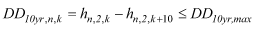 n = 1,ndd (5)
 n = 1,ndd (6)
 n=1,nsr (7)
 (8)
(8)
 (9)
(9)
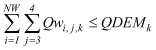 (10)
(10)
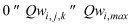 (11)
(11)