|
WRIR 99-4079: Estimates of Ground-Water Discharge as Determined from Measurements of Evapotranspiration, Ash Meadows Area, Nye County, Nevada |
||
|
|
|
|
In most arid and semi-arid environments, water is scarce and vegetation sparse to nonexistent. Ash Meadows, although a desert community, abounds in water and vegetation relative to its surroundings. The water sustaining the vegetation, shallow water table, springs, and flowing drainage channels throughout the local area is derived almost entirely from ground water, much of which is lost to the atmosphere through ET. Evapotranspiration is a process by which water from the earth's surface is transferred to the atmosphere. The transfer requires that water change state from a liquid to a vapor, and in so doing it consumes energy. As a result, any change in the rate of water loss by ET is reflected by a change in energy. This relation between water loss and energy consumption is the basis for many of the methods used to estimate ET.
The energy at the surface of the earth can be described by the energy budget, which balances the incoming and outgoing energy fluxes. Assuming that energy terms related to biological processes and the storage of heat in the plant canopy are negligible, the energy budget for conditions typical of Ash Meadows can be expressed mathematically in terms of its principal component energy fluxes as
|
Rn = H + G + lE |
(1) |
| where | Rn is net radiation (energy per area per time); |
| H is sensible heat flux (energy per area per time); | |
| G is subsurface heat flux (energy per area per time); and | |
| lE is latent heat flux (energy per area per time), where l is latent heat of vaporization for water (energy per mass), and E is rate of water evaporation (mass per area per time). |
Net radiation (Rn) is the principal source of the energy available at the surface of the earth and is the algebraic sum of the incoming and outgoing long- and short-wave radiation. Net radiation can be expressed as
|
Rn = ( RSi - RSo ) + (RLi - RLo) |
(2) |
| where | RSi is incoming short-wave radiation (energy per area per time); |
| RSo is outgoing short-wave radiation (energy per area per time); | |
| RLi is incoming long-wave radiation (energy per area per time); and | |
| RLo is outgoing long-wave radiation (energy per area per time). |
Subsurface heat flux (G) is the rate of change at which heat is stored in the soil or water profile directly beneath the earth's surface. For soil, subsurface heat flux can be expressed as
|
G = HFs + {dTs dbls rBs [Cs + (W Cw)]} |
(3) |
| where | HFs is heat flux through soil at some measurement depth (energy per area per time); |
| dTs is change in soil temperature between surface and soil heat flux measurement depth per unit time (temperature per time); | |
| dbls is depth below land surface at which heat flux is measured (length); | |
| rBs is bulk density of soil (mass per volume); | |
| Cs is specific heat of dry soil (energy per temperature per mass); | |
| W is gravimetric soil water content (dimensionless); and | |
| Cw is specific heat of water (energy per temperature per mass); |
and for water as
|
G = dTw dbws rw Cw |
(4) |
| where | dTw is change in water temperature per unit time (temperature per time); |
| dbws is depth below water surface over which temperature is measured (length); and | |
| rw is density of water (mass per volume). |
Net radiation and subsurface heat flux can be measured or computed in the field using readily available instrumentation. The difference between these two components is the energy available for sensible and latent heat flux at the earth's surface. Equation 1, which describes the energy budget as components of net radiation, can be rearranged as
|
Ea = H + lE = Rn - G |
(5) |
where Ea is available energy (energy per area per time).
Sensible heat flux (H), the energy that goes into heating the air, is proportional to the product of the temperature gradient and the turbulent transfer coefficient for heat, and can be expressed as
|
H = ra Ca kh dT/dzt |
(6) |
| where | ra is density of air (mass per volume); |
| Ca is specific heat of air at a constant pressure (energy per mass per temperature); | |
| kh is turbulent transfer coefficient of heat in air (area per time); and | |
| dT/dzt is temperature gradient near the earth's surface, where T is temperature and zt is height at which temperature is measured. |
Latent heat flux (lE), which is the energy consumed for evapotranspiration and is proportional to the product of the vapor pressure gradient and the turbulent transfer coefficient for vapor, can be expressed as
|
lE = (l ra e kv / P) de/dze |
(7) |
| where | e is ratio of molecular weight of water to dry air (dimensionless); |
| kv is turbulent transfer coefficient of vapor (area per time); | |
| P is ambient air (barometric) pressure (force per area); and | |
| de/dze is vapor pressure gradient near the earth's surface, where e is vapor pressure (force per area) and ze is height at which vapor pressure is measured. |
Neither sensible (H) nor latent (lE) heat flux, as expressed in equations 6 and 7, can be determined directly unless the turbulent transfer coefficients are known. However, an indirect method for solving the energy budget equation was developed by Bowen (1926).
Rearranging equation 5, latent heat can be expressed as
|
lE = Ea / [(H/lE) + 1]. |
(8) |
Bowen realized from this equation that if the turbulent transfer coefficients in equations 6 and 7 are equal, the ratio between sensible and latent heat flux can be expressed as
|
H/lE = [(PCa) / (l e)] [(dT/dz) / (de/dz)]. |
(9) |
Recasting temperature and vapor pressure differentials as finite differences over two reference heights, equation 9 reduces to
|
H/lE = [(PCa) / (l e) ] [(Tl - Tu) / (el - eu)] |
(10) |
| where | Tl,u is temperature at lower or upper reference point; and |
| el,u is vapor pressure at lower or upper reference point (force per area). |
The ratio (PCa) / (l e) is referred to as the psychrometric constant (gc). The ratio is known to be nearly constant for a given altitude and can be approximated by a function of air pressure and temperature (Fritschen and Gay, 1979).
The ratio between the sensible and latent heat flux, H/lE, as expressed in equation 10, has come to be known as the Bowen ratio (b). Substituting the Bowen ratio into equation 8, latent heat flux can be expressed as
|
lE = Ea / {gc [(Tl - Tu) / (el - eu)] + 1}. |
(11) |
Evapotranspiration, the mass flux of water associated with the latent heat flux, can be expressed as
|
ET = lE / (l rw) |
(12) |
where ET is the rate of evapotranspiration (length per time).
Substituting equation 11 into equation 12, ET can be expressed as
|
Ea / (l rw) {gc [ (Tl - Tu) / (el - eu)] + 1} |
(13) |
Knowing or assuming that:
ET can be readily calculated from measurable micrometeorological data. Equation 13 was solved with data measured in the field locally and provided the primary method by which evapotranspiration was estimated at selected locations throughout Ash Meadows.
Some conditions exist for which the Bowen ratio becomes unstable. One such condition is when the Bowen ratio approaches -1. When this occurs, the equation expressing latent heat as a function of the Bowen ratio (eq. 8) approaches infinity. This and other potential errors associated with applying the Bowen ratio to solve the energy budget are not discussed in this report but can be found in standard texts and in a paper by Ohmura (1982).
Other energy-budget formulations based on variations of Bowen ratio and energy-combination methods were used to validate and provide independent checks on estimates calculated by equation 13. In general, each of these formulations solve the energy budget by computing latent and sensible heat fluxes indirectly. This report does not provide the theoretical derivation of each of the formulations--instead interested readers are referred to their published sources (Monteith, 1973; Shuttleworth and Wallace, 1985; Shuttleworth and Gurney, 1990; Nichols, 1991, 1992; G.A. DeMeo, U.S. Geological Survey, written commun., 1998).
Ten sites were selected and instrumented to measure ET from areas dominated by the different vegetation and soil conditions found throughout Ash Meadows. Other factors influencing the selection and location of a site were year-round accessibility and adequate fetch. Generally, fetch is defined as the distance between the sensor and the upwind edge of the environment of interest and implies a homogeneous mix of vegetation types, soils, surface water, or some combination thereof. Sites were located such that the fetch was at least 100 times the height of the highest temperature-humidity sensor (Campbell, 1977). The location and general description of the sites selected for instrumentation are given in table 6.
With one exception, sites were located such that each ET unit was represented by at least one site. The lone exception was the ET unit referred to as submerged aquatic vegetation (SAV, table 3). Although spectrally unique, SAV is only 81 acres and is assumed to evapotranspire water at a rate equal to that of open water (OWB, table 3). Multiple sites were located in certain units to evaluate the potential for differences in the rate of ET associated with intra-unit changes in vegetation or soil conditions. Three sites were located in the largest unit (7,160 acres, pl. 1) defined as sparse grassland vegetation (SGV). Two sites each were located within the units defined as dense grassland vegetation (DGV) and moist bare soil (MBS). Time constraints, accessibility issues, and instrumentation difficulties did not allow for the individual evaluation of every intra-unit change in vegetation or soil conditions.
Each site was equipped with the instrumentation required to measure or compute the micrometeorological data needed to calculate the energy-budget fluxes by the several methods discussed. A schematic showing the typical instrument arrangements used to determine ET over land and over water is shown in figure 8. Photographs of actual land and water-based installations are presented in figure 9. A typical land-based installation consists of a net radiometer to measure net radiation; two solid-state air temperature/humidity probes to measure air temperature and relative humidity; two anemometers to measure windspeed; two infrared temperature sensors to measure soil and plant canopy temperatures; and a set of thermocouples and heat flux plates to compute soil heat flux (fig. 8). Instrument pairs are used to measure vertical differences of a particular variable between two reference heights. Initially, vapor-pressure gradients were computed from dew-point temperatures measured by pumping air from two reference heights through a single chilled-mirror hygrometer (Tanner and others, 1987). During the early part of the study, the hygrometer was found to be unreliable over extended time for many of the climatic conditions being measured. To remedy this problem, one of two modifications were made to the instrumentation. Either the chilled mirror hygrometer was replaced with a solid-state temperature/humidity probe or was replaced with individual temperature/humidity probes to measure relative humidity and temperature at two reference heights. In the two-probe setup, instrument positions were exchanged once during a data acquisition interval (20 minutes) to cancel any bias that may exist between the individual probes (Fritschen and Simpson, 1989; Fritschen and Fritschen, 1993). Readers interested in additional discussion of the instrumentation applied in this study are referred to Nichols and Rapp (1996).
An ET site established over open water uses similar instrumentation but has a slightly different instrument arrangement (fig. 8). The major differences are related to the presence of water. For open water, the temperature and vapor pressure gradients are not measured between two reference heights in the air but rather between one reference height in the air and the water surface. Thus, only one temperature/humidity probe is required for air temperature and relative humidity measurements. Temperature at the water surface is measured with an infrared temperature transducer, and assuming that the air is saturated at the water surface, vapor pressure is computed as the saturation vapor pressure. Another difference affecting the general setup is that subsurface heat flux was not calculated with heat flux plates but rather using temperature probes set below the water surface to compute changes in heat storage (eq. 4). Heat-storage changes were computed only for the upper 2 ft of the water column and changes from greater depths were assumed insignificant to the overall energy budget.
Micrometeorological data required to solve the energy budget by the methods discussed previously were collected at each of the ET sites for a minimum of 1 year, which is considered the minimum period by which seasonal fluctuations in evapotranspiration rates can be evaluated and documented. Multiple years of data were acquired at some sites to assess annual changes in ET that may result from climate variations, such as differences between dry and wet years. The period of data acquisition for each instrumented site is given in table 6.
The micrometeorological data collected throughout the study were stored as 20-minute averages computed from measurements made during 10 or 30-second sampling intervals. The collection process produced large amounts of data, which are not presented in the report but are available upon request from the U.S. Geological Survey (Las Vegas office). Gaps in the record occurred as a result of instrument failure and the inability of specific instruments to make accurate measurements under certain climatic conditions. ET was calculated from energy fluxes measured and computed from the Bowen ratio for each 20-minute interval, except for those intervals having missing or inaccurate data or during which the Bowen ratio solution was unstable. A typical set of micrometeorological data acquired to solve the energy budget is shown in figure 10 for the 5-day period, September 1-5, 1996, at CMEADW (table 6, pl. 1).
Daily ET was computed by summing ET calculated for each 20-minute period. Daily values were computed only for days having 68 or more 20-minute computations. Energy-budget fluxes and daily ET calculated from the Bowen ratio at CMEADW for the 5-day period, September 1-5, 1996, are shown in figure 11.
Daily ET calculated by the Bowen ratio method at CMEADOW for 1996 is shown in figure 12. The minimum calculated daily ET is near zero on day 326 (November 21) and the maximum is nearly 0.25 inch on day 198 (July 16). The mean of the daily ET values is 0.097 inch. Annual ET for 1996 is 35.4 inches and was computed by integrating the daily ET values calculated for the year. Although a plot of daily ET values shows a general pattern defined by higher rates throughout the late spring and summer months, daily variability is evident (fig. 12A). Daily variability is due mainly to short-term changes in weather patterns. Smoothing the annual ET curve using an eighth-order polynomial fitted to daily ET values reduced daily variability while reasonably maintaining the annual value of ET as calculated directly from the daily values. The smoothed annual ET curve for 1996 at the CMEADW site is compared to computed daily ET values in figure 12A. Annual ET calculated by integrating the smoothed ET curve is 35.5 inches and compares favorably to annual ET calculated from daily values (35.4 inches). The smoothed ET curve is assumed to better represent daily fluctuations over a typical year and allows for clear graphical comparisons of ET rates computed by different methods, for different sites, and over multiple years. Any small differences between the smoothed and computed daily ET values shown on figure 12 for the first few and last few values are attributed to artifacts of the fitting algorithm.
Smoothed ET curves calculated from daily ET values computed by other methods are compared to the Bowen ratio curve for 1996 at the CMEADW site in figure 12B. Annual ET computed by the different methods identified in the figure ranged from 28.9 to 35.5 inches. Although the comparison shows some differences, the overall agreement between the methods is considered reasonable. As stated previously, these other methods were used only as independent checks to validate the reasonableness of the Bowen ratio method.
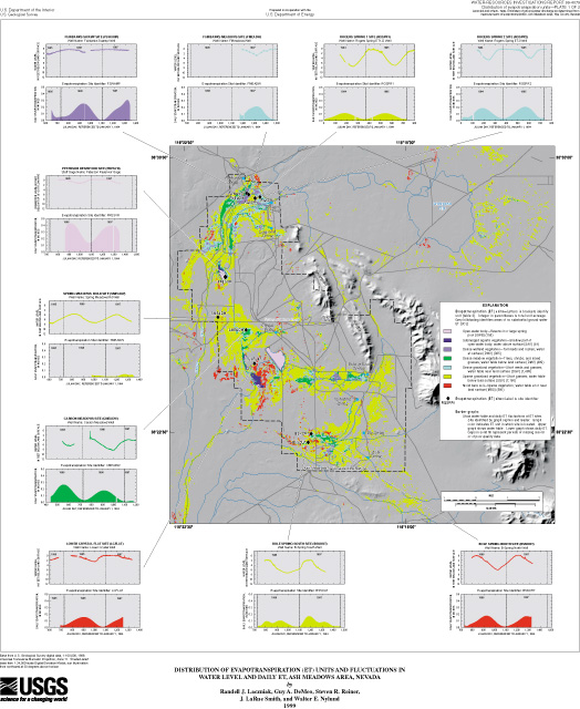
ET curves developed from data collected at each of the instrumented ET sites are shown on plate 1. An estimate of the average annual ET at each site, which was computed by integrating its ET curve over a 1- or 2-year period, is given in table 7. Estimated average annual rates differed between ET units and ranged from 8.60 ft over open water (Peterson Reservoir, PRESVR) to 0.62 ft over sparse saltgrass (Spring Meadow, SMEADW). A graph combining all ET curves for the period of data collection is shown in figure 13. The figure also shows annual precipitation determined from volumetric rainfall measurements taken during 1995, 1996, and 1997 near Rogers Spring 1 (RGSPR1) site (pl. 1). Annual precipitation for the 3-year period ranged from 2.4 inches in 1996 to 4.8 inches in 1995.
The aggregate graph of ET curves (fig. 13B) shows the spatial and temporal differences in ET computed throughout the Ash Meadows area. The individual curves show some significant differences in computed daily and annual ET rates between ET units and also show some differences between multiple sites within an ET unit. Intra-unit differences are greatest in SGV where annual ET ranges from 0.62 ft at Spring Meadow (SMEADW) site to nearly 2 ft at Bole Spring South (BSSOUT) and Rogers Spring 1 (RSPRG1) sites. Although temporally limited, ET rates computed for some sites exhibit daily and annual (year to year) variations. Annual variation is most apparent at Carson Meadows (CMEADW) site (fig. 13B) and may be explained in part by differences in precipitation. The ET curve for the CMEADW site indicates higher daily and more annual ET in 1995 than in 1996. The higher rates are consistent with precipitation being greater (by a factor of 2) in 1995 than in 1996, and are likely a response to an increase in water availability. Similarly, the ET curve for the Fairbanks Swamp (FSWAMP) site indicates higher daily rates and more annual ET in 1997 than in 1996.
The ET curve for BSSOUT defines dual ET peaks over each measured calendar year (fig. 13B). The first peak can be explained by the presence of standing water that inundates the site during late winter and early spring, and eventually evaporates or drains away. The later peak is likely the typical late spring/early summer peak associated with a period of maximum plant vigor. Although the dual peaks are apparent in the 1996 and 1997 records, the higher initial peak in 1997 is attributed to a greater amount and a prolonged presence of surface water in the early part of 1997.
One rather anomalous result is the large ratio (in excess of 2) between the open-water evaporation (8.60 ft/yr, fig. 13B) and wetland evapotranspiration (3.91 ft/yr, fig. 13B). Typically this ratio is assumed to be about one (Hammer, 1989, p. 27). This assumption is based on results of several studies (Christiansen and Low, 1970; Kadlec, 1986; Kadlec and others, 1988), all of which were done in more humid and cooler climates. The annual ET determined for dense wetland vegetation is near that measured in these other studies, thus the high ratio is attributed to the higher open-water rate. A higher open-water rate would be expected considering the other regions' climatic conditions. Another factor contributing to the higher ratio is that the dense mat of dead vegetation (1 to 3 ft thick) and the marsh plant structure (tall and broad-leafed) work together to reduce evaporative losses. The reduction is caused by shading of the water surface and by limited air movement through the vegetative cover (Hammer, 1992, p. 28). Shading effects can drastically reduce winter evaporation as is shown by comparing the winter parts of the PRESVR and FSWAMP daily ET curves in figure 13B. Stagnant air creates conditions where the relative humidity is near saturation throughout the thick vegetative covering, minimizing any exchange with drier air. Together these factors are likely accountable for the atypical ratio between open-water and wetland evapotranspiration.
|
|
|