GROUND-WATER DISCHARGE

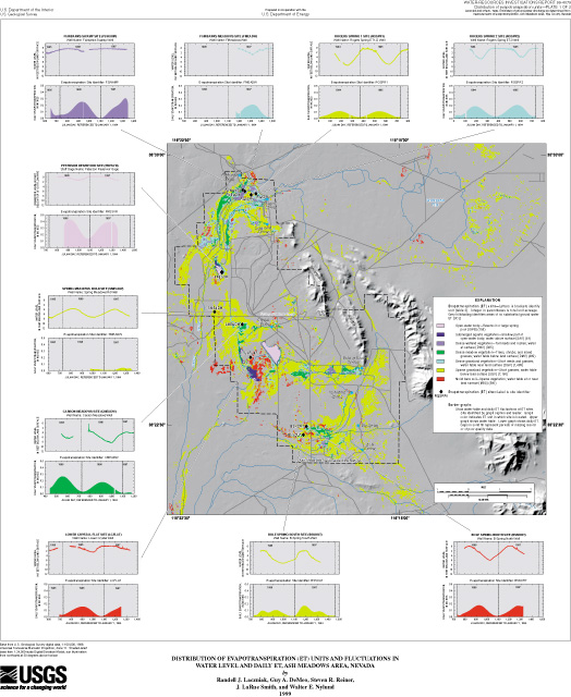
Ground water leaves the Ash Meadows area by four major processes: (1) springflow, (2) transpiration by local vegetation, (3) evaporation from soil and open water, and (4) subsurface outflow. Another process, although unnatural, by which ground water has been removed from the system is through pumping for local water supply. Since the early 1980's, pumping from the local area is minimal. Of all these processes, springflow is the most visible form of discharge (see section "General Hydrology," fig. 4). As ground water emerges from the orifices of the many springs scattered about the area, it either is pooled or is channeled into free-flowing drainages or local reservoirs. Once at the surface, water evaporates into the atmosphere or disperses outward and downward into the valley-fill deposits. Little if any surface water flows beyond the boundaries of Ash Meadows except during short periods (less than a few days) following occasional, intense rainfall.

Most of the spring and surface flow percolating downward into the valley-fill deposits recharges a shallow ground-water system (fig. 4). This flow system, referred to as the valley-fill aquifer, is bounded on top by a shallow water table and below by underlying carbonate bedrock. In addition to recharge from above, this aquifer also is recharged from below by diffuse upward flow from the underlying regional carbonate-rock aquifer. Other than the occasional influx of water from rainfall, these two sources of recharge provide most of the water maintaining the shallow, valley-fill aquifer. As with the regional carbonate-rock aquifer, some portion of ground water is likely to move southwestward across the Ash Meadows fault system and into the adjacent valley-fill deposits in the central part of the Amargosa Desert. Subsurface outflow is likely to be small owing to the relatively low permeability of adjacent valley-fill deposits. The remainder of the water is stored locally within the valley-fill aquifer, and in areas where the water table is at or near the surface, becomes available for use by plants and is exposed to atmospheric processes. Water evaporated directly from the plant structure is called transpiration and that evaporated from the soil structure is bare soil evaporation. Together these terms are referred to as evapotranspiration or ET. Evapotranspiration is the primary process by which ground water is removed from the valley-fill aquifer. Temporal differences in the relative amounts of water entering and leaving the valley-fill aquifer are indicated by changes in the water table. If more water enters than leaves the aquifer, the water table rises; and conversely, if more water leaves than enters, the water table falls. Seasonal changes in ET are responsible for the large seasonal fluctuations in the local water table--generally a declining water table in the summer and fall, and a rising water table in the winter and spring.

Most previous attempts to quantify ground-water discharge from Ash Meadows have been based primarily on measurements of springflow. Long-term annual estimates of ground-water discharge range between 16,500 and 17,500 acre-ft (Walker and Eakin, 1963; Winograd and Thordarson, 1975, p. 84; Dudley and Larson, 1976, p. 12). Although these "springflow" based estimates of ground-water discharge account for most of the water discharging by way of springs, the approach does not account for inflow to the valley-fill aquifer by subsurface seeps or by diffuse upward flow from below, across the surface of the underlying carbonate-rock aquifer. Assuming that subsurface outflow is small, one alternate method of estimating the loss of ground water from the Ash Meadows area is to quantify local ET from the general areas of ground-water discharge. An estimate of ET includes water losses from the regional carbonate-rock aquifer both by diffuse upward flow into the shallow valley-fill aquifer and by spring discharge. The ET estimate includes spring discharge because most springflow is evaporated or recycled back into the subsurface where it recharges the shallow valley-fill aquifer and eventually either is evaporated or transpired by the local vegetation.

Past estimates of ET from Ash Meadows were completed as part of regional assessments of the ground-water resource. Long-term annual ET estimates were computed from generalized delineations of phreatophyte growths and adaptations of annual ET rates for similar plant assemblages found throughout the western United States (Lee, 1912; White, 1932; Young and Blaney, 1942). Applying generalized acreages and ET rates, Walker and Eakin (1963, p. 22) estimated 24,000 acre-ft of annual ET over the entire Amargosa Desert. Of this total, about 10,500 acre-ft was determined to be from Ash Meadows (Winograd and Thordarson, 1975, p. 84); and the remainder from other smaller areas of ground-water discharge found throughout the Amargosa Desert. By comparing springflow and ET estimates, Winograd and Thordarson (1975, p. 84) suggest that ground water lost through transpiration by phreatophytes and evaporation from bare soil may be derived entirely from recycled springflow--but also discuss the likelihood of upward flow from the underlying carbonate-rock aquifer as being a source of the water supporting the area's phreatophyte population. These authors explicitly state that this quandary can only be resolved with a detailed study of evapotranspiration. This recommendation, the significance of quantifying ground-water discharge in terms of formulating an understanding of ground-water flow, and results from recent studies (Johnson, 1993; Nichols and others, 1997) suggesting that ET rates for local phreatophytes may be higher than those given in Walker and Eakin (1963, p. 23), provided the motivation to initiate a study to re-evaluate and more rigorously quantify ET from the Ash Meadows area.

This study of ET at Ash Meadows accounts only for ground water lost to the atmosphere. The estimates given do not account for ground water consumed at the refuge for operational needs, by the few local residents for domestic purposes, or by the local wildlife; or that which escapes the area as subsurface outflow. Currently, consumed water is minimal and probably does not exceed more than 10 acre-ft/yr. Previous estimates of subsurface outflow vary and range from zero to less than a few hundred acre-feet annually (Czarnecki and Waddell, 1984, table 1; Prudic and others, 1995, p. 62). The inclusion of these minor discharge components in the overall ground-water discharge estimate would likely be only a small fraction of the total. The estimation of these components is beyond the scope of this particular effort.

Quantification of Evapotranspiration

The basic method used to quantify evapotranspiration from the Ash Meadows area is similar to the approach applied previously by Walker and Eakin (1963). The methodology assumes that total ET can be quantified by summing individual estimates of annual ET computed for areas of similar plant (type and density) and soil (type and moisture content) cover. Hereafter, these areas of similar vegetation and soil conditions are referred to as ET units. An estimate of annual evapotranspiration for each ET unit is computed by multiplying the unit's acreage by an appropriate estimate of ET for the unit's vegetation and soil conditions. The major difference between previous estimates and the estimate presented in this study is in the specific techniques used to identify individual ET units, determine their spatial distribution, and estimate their associated ET rates. The techniques applied in this study take advantage of more modern technologies and are expected to result in a more accurate characterization. Previous methods defined and delineated ET units and their associated acreage on the basis of fairly generalized vegetation and soil mapping; whereas this study refines this approach by utilizing satellite imagery and remote sensing techniques. Evapotranspiration rates estimated in previous studies were based on measurements made for similar phreatophytes found at locations outside the study area; whereas this study made direct measurements of ET at locations within Ash Meadows. Because local vegetation and soil conditions in the Ash Meadows area are largely a consequence of the availability of ground water, water levels also were measured to define the depth and annual fluctuation of the water table.

Evapotranspiration Units

Evapotranspiration (ET) units were identified and mapped in the Ash Meadows area through a procedure by which spatial changes in vegetation and soil conditions were determined by classifying remotely sensed spectral data on the basis of similarities and patterns in spectral-reflectance characteristics. The procedure used Landsat Thematic Mapper (TM) imagery as the primary source of spectral data (fig. 5). TM imagery is acquired by satellites equipped with sensors that collect spectral information. The satellite measures reflected solar and emitted radiation from the Earth's surface and that scattered from the atmosphere. Measurements are made within seven wavelength bands spanning discrete parts of the visible and infrared regions of the electromagnetic spectrum. Each band is referred to as a TM channel. Six TM channels (1, 2, 3, 4, 5, and 7) measure reflected solar radiation in the visible, near infrared, and short wave infrared regions (fig. 6A). A seventh band, TM channel 6, measures thermal energy emitted from the surface of the Earth in the thermal infrared region, and is not used in this procedure.

Spectral data received by the satellite sensors are transmitted to earth as digital numbers, each denoting the reflectance of the wavelengths within a TM channel from a small area of the earth's surface. The surface area scanned by the sensor for TM channels 1, 2, 3, 4, 5, and 7 measures about 100 ft by 100 ft. Each square-shaped area is referred to as a picture element or pixel. The dimensions of these pixels define the spatial resolution of the imagery. One major benefit of these digital data sets or images is that they can be manipulated, processed, and geographically referenced using sophisticated computer algorithms.

Satellite data have long been used for identification and delineation of different land covers (Anderson and others, 1976, p. 2; American Society of Photogrammetry, 1983, p. 23-25). Vegetation, water, and soil covers have distinct spectral properties and can be identified by characteristic patterns or signatures defined by their spectral-response curves (fig. 6). A closer analysis of the shape, slope, and absorption features within a land cover's spectral-response curve often can be used to identify differences in vegetation type, density, and health, and differences in soil type and moisture content (Goetz and others, 1983, p. 576-581). Past studies have shown that ET rates throughout the Great Basin region vary with vegetation and soil conditions--in general, the denser and more healthy the vegetation or the wetter the soil, the greater the rate of evapotranspiration (Ustin, 1992; William D. Nichols, U.S. Geological Survey, written commun., 1998). The procedure used to identify and map the ET units in the Ash Meadows area takes advantage of this relation and the characteristic patterns inherent in the spectral-response curves of differing vegetation and soil covers, particularly those associated with the evapotranspiration of ground water.

Spectral Classification

The process of identifying pixels on the basis of patterns in their reflectance spectra is referred to as a classification. If pixels are grouped to represent specific land covers, the classification is called a land-cover classification and each different land cover defines a unique class. The procedure presented here ultimately groups pixels into specific ET units, and thus is referred to as an ET-unit classification. The procedure independently classified two TM images of the Ash Meadows area into land covers representing the different vegetation and soil conditions likely to be associated with areas of ongoing ground-water ET. The dual classifications accounted for changes in vegetation and soil conditions occurring through a typical year. One image, taken June 13, 1992 (scene identification number LT5040035009216510, fig. 5), represents conditions of near maximum plant vigor and of high moisture, a period when the water table was near its highest level. The other image, taken September 1, 1992 (LT5040035009224510), represents conditions of high plant stress (dormancy) and of low moisture, a period when the water table was at or near its lowest level. The two classified images were combined to formulate a single map defining the spatial distribution of ET units throughout the Ash Meadows area (pl. 1).

The first step in classifying ET units was to determine the basic vegetation and soil conditions associated with each pixel in the imagery. The procedure applied a multi-spectral, maximum-likelihood classification using an unsupervised approach (Lillesand and Kiefer, 1987, p. 685-689). The unsupervised approach identifies the unique spectral responses present within the imagery as defined by TM channels 1, 2, 3, 4, 5, and 7. The approach determines the number of unique spectral-response curves within each image. Uniqueness is based on statistical similarities between reflectance values in the TM channels of individual pixels. Each curve is defined by statistical variables representing a unique set of reflectance values. An example comparing the spectral response or signature of different vegetation and soil conditions is shown in figure 6A. These same spectral signatures as developed from percent reflectance for the TM channels analyzed are shown in figure 6B.

Next, the procedure determined the spectral-response curve that best represented each pixel in the June and September imagery. The determination was made using the maximum likelihood classification technique. This technique compares reflectance values of each pixel against the signature defined by each spectral-response curve and calculates the statistical probability of a pixel being represented by each of the different spectral-response curves. Each pixel was assigned the number of the spectral-response curve having the greatest probability.

The next step in the process was to group spectral-response curves into clusters defining general vegetation and soil conditions. Spectral-response curves were grouped on the basis of similarities in the statistics defining their reflectance values. Each individual group is referred to as a spectral cluster and is discriminated by characteristic patterns described in the response of the cluster's reflectance values. Patterns are distinguished by differences in a spectral-response curve's slope between TM channels, or by sharp dips in the curve indicating absorption at a particular TM channel. The spectral signatures characteristic of pixels falling within areas dominated by open water, phreatophytes, and moist bare soils were used to define six spectral clusters representing the different vegetation and soil conditions consistent with likely areas of ground-water evapotranspiration. In addition to these six spectral clusters, the signatures characteristic of pixels falling in areas dominated by sparse upland desert vegetation or in xeric habitats were used to define the spectral cluster representing areas of no substantial ground-water ET. Each cluster was given a number to digitally differentiate each of the conditions of interest. A description of each of the seven general land-cover clusters (and one unclassified area) is given in table 1. The spectral clusters defining the six different vegetation and soil conditions representing likely areas of substantial ground-water ET are shown in figure 7 for the June and September imagery.

Open water was determined independently for both dates from an August 8, 1993, SPOT (Systeme Probatoire d'Observation de la Terre) image. SPOT imagery provides spectral data at a much finer spatial resolution (about 60 ft by 60 ft) than TM imagery but contains spectral information only in the visible and near infrared regions of the electromagnetic spectrum. SPOT imagery lends itself well to discriminating open water, but was found to be less effective in discriminating land covers representative of ET units throughout the Ash Meadows area.

The final step in the ET-unit classification combined the two independently classified images into a single digital image defining ET units and their spatial distribution. The cluster combinations resulting from combining the June and September classifications provided the basis for assigning and identifying ET units. The number of pixels assigned to each cluster combination is shown in table 2. In this table, rows identify the number of pixels assigned to each spectral cluster by the June classification, and columns identify the number of pixels assigned to each spectral cluster by the September classification. For example, a value of "2" in the third row (cluster 2) and the second column (cluster 1) indicates that only two pixels were classified as cluster 2 from the June imagery and cluster 1 from the September imagery.

The spatial resolution of pixels given in table 2 is much finer than that of the original TM imagery. The finer resolution was attained by re-sampling the original images at a pixel spacing of about 60 ft by 60 ft. The re-sampling does not provide more spatial detail but allowed for the direct integration of the TM and SPOT imagery (which was used to classify open-water bodies).

The major differences between the June and September classifications are apparent when comparing cluster combinations defined by the row and column values in table 2. If the two classifications were identical, all non-bolded elements in table 2 would be zero. The sum of the integer values in the non-bolded elements indicates the number of pixels assigned to different ET units by the two classifications. Some of the differences can be attributed to errors in the image registration, but most are likely to be the result of changing vegetation and soil-moisture conditions between the time of year during which the images were acquired. Most differences noted in the table can be explained in terms of expected seasonal changes. For example, the greater number of pixels assigned to non-zero clusters by the June classification implies a larger area of ground-water ET. This implication is consistent with field observations that indicate a greater availability of accessible ground water and more vigorous plant growth in June than in September. The one exception to this overall trend is the large number (15,899) of pixels classified as sparse vegetation (cluster 4) in the September image and as areas of no substantial ground-water ET (cluster 0) in the June image (table 2). This inconsistency arises by the omission of a few spectral-response curves from cluster 4 in the June classification. These spectral-response curves were omitted purposely because, if included, would classify vegetation dominated by non-phreatophytic species (such as saltbush and desert holly) as areas of ground-water ET (cluster 4). Instead, the September classification was used to define the outer boundary of sparse phreatophyitic vegetation. Classification of areas dominated by non-phreatophytic plant species based on the June imagery can be explained by the vigor of these species during late spring and early summer.

Each cluster combination was evaluated on the basis of field observations and its spectral-reflectance characteristics. The evaluation process identified seven ET units (table 3) that preserved the general spectral and physical characteristics of the original land-cover designations (table 1), with two exceptions. One difference was that class 4 (sparse vegetation, table 1) and class 6 (previously farmed field, table 1) were combined into one unit (SGV, table 3) on the basis of similarities in vegetation, general soil conditions, and depth to water. The other major difference was the creation of a unit to discriminate areas of dense wetland vegetation (DWV, table 3). The reclassification scheme used to assign an ET unit to each pixel is given in table 4. In this table, rows represent cluster classifications as determined from the June imagery, and columns represent cluster classifications determined from the September imagery. The ET-unit designator (described in table 3) given for each cluster (row, column) combination is the ET unit that was assigned to each pixel on the basis of both the June and September classifications. For example, the ET-unit designator SAV (submerged aquatic vegetation) assigned to the cluster combination (2,1) implies that all pixels classified as cluster 2 from the June imagery and cluster 1 from the September imagery (table 2) were reclassified as SAV.

After being reclassified, the image was smoothed using a nominal filter. In general, the filter replaced spurious classified pixels (areas defined by less than three adjacent pixels) in the image and filled single-pixel gaps within delineated ET areas by assigning them to the ET unit most representative of its neighbors. The final map delineates 10,352 acres of ongoing ET in the Ash Meadows area. The acreage and spatial distribution of individual ET units are given in plate 1. The largest ET unit, defined as sparse grassland vegetation, covers 7,160 acres; whereas the smallest ET unit, defined as submerged aquatic vegetation, covers only 81 acres.

Accuracy Assessment

The ET units, as defined and delineated, are not intended to be exact but rather generalizations of the long-term average conditions. The accuracy of the final ET-unit classification is difficult to assess because the vegetation and soil conditions throughout the Ash Meadows area are not homogeneous, and transitions from one condition to the next are not abrupt but rather subtle and often occur over broad zones. Another factor contributing to the difficulty in assessing the accuracy of mapped ET units is that the vegetation and soil conditions change during a year and from year to year. Despite these difficulties, an assessment of the overall accuracy was made of the ET-unit classification.

The overall accuracy of the final ET-unit map (pl. 1) was assessed by comparing units assigned on the basis of field observation with those assigned by the classification procedure. Comparisons were made at 30 sites. Each ET-unit was represented by at least one site in the assessment. Assessment locations included the sites established to measure ET rates (pl. 1). A field observation included one or more site visits to examine and document actual site conditions. Each site was described, photographed, and later evaluated and assigned to one of the seven ET-units independently by two individuals. The few discrepancies in class assignments were resolved through discussion and site re-visitation.

The overall performance or accuracy of a classification procedure can be described in terms of the percentage of sites classified correctly (Lillesand and Kiefer, 1987, p. 692-694). A correctly classified site is one in which the same ET unit is assigned both through field observation and by the classification procedure. An assessment of the accuracy of the final ET-unit classification is presented as a contingency table (table 5). The table shows the number of sites assigned to each ET unit by field observation (row) and by classification (column). The value "14" given in the row-column combination of SGV (sparse grassland vegetation) in table 5 indicates that 14 of the evaluated sites were assigned to SGV (sparse grassland vegetation) both by field observation and by classification. The three values of "1" in this same row indicate that three additional sites were assigned to SGV by field observation but were assigned incorrectly to DWV (dense wetland vegetation), DMV (dense meadow vegetation), and DGV (dense grassland vegetation) by classification. On the basis of this example, 14 of the 17 sites assigned to SGV by field observation also were assigned by classification to SGV for an accuracy of 82 percent. The performance of the classification procedure for individual ET units ranged from 67 to 100 percent (table 5). The overall performance of the assessment is 86.6 percent, where performance is defined as the ratio of the number of sites assigned correctly by classification (26) to the total number of sites evaluated (30). This performance is within the acceptable limit (85 percent or greater) established by Anderson and others (1976, p. 5).

Table 5 indicates that the lowest performing class is dense meadow vegetation (DMV, table 3). The low performance of this class could be related to the limited number of sites evaluated (3), or rather may be attributed to the class being comprised largely of mixed vegetation covers--trees, shrubs, and grasses. The mixed and differing vegetation associated within this class yield a less distinctly defined spectral cluster (fig. 7, cluster 2) making its classification more ambiguous. The discrepancy between the observed and classified site assignments is considered acceptable because both procedures assigned the site in question to a unit of dense vegetation -- dense wetland vegetation (DWV) by classification and dense meadows vegetation (DMV) by observation. The average of the individual class performances is 91.5 percent (table 5), also suggesting an acceptable ET-unit classification of the Ash Meadows area.