U.S. Geological Survey Data Series 722
In general the acquisition hardware for this survey included four components: a GPS base and GPS rover, a motion sensor (vessel heave, pitch, and roll), and an echosounder. On the RV Survey Cat, the single-beam transducers are sled mounted and ride on a rail that is attached between the catamaran hulls. During surveying the sled is pulled forward and secured into a position located directly below the GPS antenna (fig. 8). The motion sensor is located along the centerline of the boat in the forward cabin. All hardware component positions on the RV Survey Cat were surveyed using a static total station while the boat was on the trailer and leveled. The base of the transducers served as the reference point. This effort provided millimeter-level accuracy for numerical offsets for post-processing.
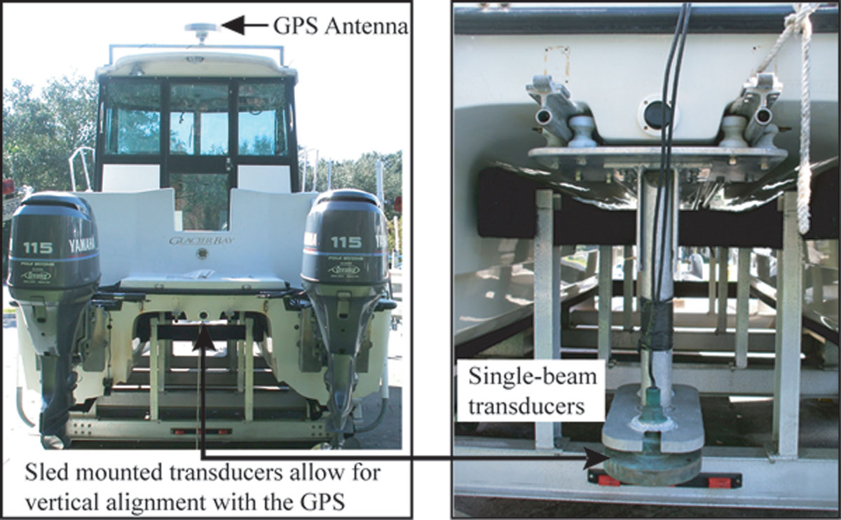
Figure 8. Photographs of the hardware components on the RV Survey Cat. [larger version] |
Depth soundings were recorded at 50-millisecond (ms) intervals using a Marimatech E-SEA-103 echosounder system with dual 208-kHz transducers. Boat motion was also recorded at 50-ms intervals using a TSS DMS-05 sensor. The bathymetry was acquired using HYPACK MAX version 4.3a.7.1 (HYPACK, Inc.), a marine surveying, positioning, and navigation software package. The data from the GPS receiver, motion sensor, and fathometer were streamed in real time to a laptop computer running HYPACK on a Windows operating system. HYPACK acquisition combines the data streams from the various components into a single raw data file, with each device string referenced by a device identification code and time stamped to the nearest millisecond. The software also manages the planned-transect information, providing real-time navigation, steering, correction, data quality, and instrumentation-status information to the boat operator.
A generalized workflow diagram of post-processing is shown in figure 9. The diagram outlines the sequence of the various inputs and processing components that result in finished map products and data archives. The software components are described in the following section.
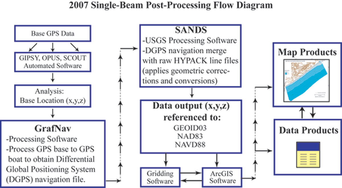
Figure 9. Diagram of the single-beam post-processing workflow indicating the progression and software components used to derive the bathymetric data and other products. [larger version] |
Establishing the differentially corrected (DGPS) external navigation file began with processing the static GPS data from the primary base station. These data may be processed quickly and accurately through one of the three online submittal services commercially available: (1) Automated GPS-Inferred Positioning System (GIPSY), a service provided by National Aeronautic and Space Administration's (NASA) Jet Propulsion Laboratory, (2) On-Line Positioning User Service (OPUS), maintained by the National Oceanic and Atmospheric Administration (NOAA) and the National Geodetic Survey (NGS), and (3) Scripps Coordinate Update Tool (SCOUT). The results from these services are put in a spreadsheet for error analysis and averaging. Any sessions that differ from the averaged ellipsoid value by more than 0.05 m are removed. The type of online service used may depend upon the survey logistics, which are defined by the project. For the 2007 bathymetry, results from all three services were analyzed independently first. The final x,y,z position from each service was then reviewed and averaged together. The SCOUT values differed the greatest from the average of the three, with 1.175 m in the vertical, whereas GIPSY and OPUS were considerably less at 0.627 m and 0.549 m, respectively. For this reason SCOUT values were not included in the final position, only GIPSY and OPUS and produced +/- 3.9 cm accuracy in the vertical component. This base station position, once finalized, was used as the base location (x,y,z) for post-processing the base GPS to the rover GPS. Table 1 lists the position for FORT used in post-processing. The data from FORT were good for the entire survey, so BH08 was not needed for processing.
| Table 1. Final base station position value for FORT. This position is the weighted average of the GPS sessions that were processed with GIPSY and OPUS.
|
|---|
| Final Base Position (USGS) | Latitude (NAD83) | Longitude (NAD83) | Weighted Ellipsoid (WGS84) | O=E-G Orthometric (m) (GEOID03/NAVD88) |
GEOID03 Utility | Error (cm) |
|---|---|---|---|---|---|---|
| FORT | 30o 12' 43.68831 | 88o 58' 19.51691 | -17.417 | 10.176 | -27.593 | +/- 3.9 |
Each base station GPS file was processed to the roving vessel using GrafNav version 7.6, a product of Waypoint Product Group. During this process, steps were taken to ensure that the trajectory produced from the base to the rover was clean and produced fixed positions. This is done through the interpretation and use of graphs, maps, and logs that GrafNav produces for each file. Some simple controls to eliminate poor GPS data at this point included, but were not limited to, excluding data from a satellite flagged by the program as having poor health, eliminating satellite time segments that have had cycle slips, and adjusting the satellite elevation mask angle. From these processes, a single quality checked, differentially corrected, precise position file at 1-s intervals was created for each vessel GPS session.
The single-beam data were processed using SANDS version 3.7. SANDS uses the time stamp to correlate the external navigation file with the HYPACK line data and performs geometric corrections on the depth values using the pitch and roll motion of the boat as recorded by the TSS motion sensor. The heave component is not used in SANDS but is more accurately represented by the GPS component (DeWitt and others, 2007; Hansen, 2008; Mark Hansen, USGS, unpub. data, 2009). SANDS also has the option to apply a geoid model and GEOID03 was also applied to the data. The end result was an x,y,z file horizontally and vertically referenced to NAD83 Universal Transverse Mercator (UTM) Zone 16 North (N) and NAVD88 orthometric height.
The processed x,y,z data were imported into ESRI's ArcMap version 9.2. The data were gridded with the 3D Analyst Interpolation to Raster tool using natural neighbors interpolation at 50-m grid cell size. From this grid, a 1-m contour surface was generated. A shapefile of the individual data points (x,y,z) was created, plotted as 1-m color coded intervals, and overlain atop the gridded and contoured surfaces. Using all three surfaces as guides helped the editor visually scan for any remaining discrepancies. For example, converging or crossing contour lines indicated problem areas, deep holes, or abnormally shallow zones that appeared in abnormal locations. All were indicators of potential false or bad x,y,z data values. Any areas identified as questionable were reviewed, and if found to be bad, values were either deleted or statically adjusted. This resulted in 102,412 x,y,z data points.
Once all data were reviewed, a final grid was generated in the same manner as above. A raster mask was created to clip the data to the extent of the survey lines (see fig. 11). The contour surface generated from the final grid was edited in ArcMap Editor, and the data points were used as a check that the contour lines passed through the correct values. If the lines did not, they were adjusted accordingly using the editing line tool. When the extent of contour editing was finalized, the contour surface was imported into Adobe MapPublisher version 5 for further smoothing and polishing of the contours. Once finished, the smoothed contour file was imported back into ArcMap and rechecked against the data points for a final verification that the lines were not improperly smoothed and were still accurately representing the 1-m contour intervals of data points.
The quality control measures for the navigation data are applied during acquisition as outlined in the
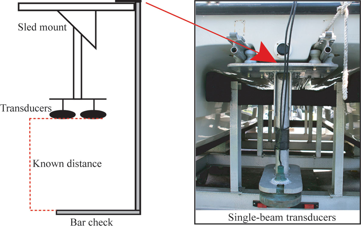
Figure 10. Diagram of a bar check. The red arrow indicates the point at which the bar is attached. The distance from the base of the transducers to the top of the bar is a known distance. The values from the echosounder are recorded and then accounted for in post-processing. [larger version] |
In theory, where two bathymetric lines cross, the data values at that point should be equal. If they are not, this could be an indication of inaccurate values or poor data. GPS cycle slips, poor weather conditions, and rough survey conditions may produce poor data. Water column sound velocities were not measured with the assumption that shallow water environments are well mixed; therefore, sound velocities would not be an issue. If discrepancies were found at the line crossings, the line in error was either statically adjusted or removed. A line in error was considered to have one or more of the following: (1) a segment where several crossings are incomparable, (2) a known equipment problem, (3) known bad GPS data evident in post-processing, which can negatively affect the final depth value. There were 251 crossing zones that yielded 298 crossing values. Some zones had more than one set of data points that could be considered. The crossing checks were considered successful and range from 0.00 - 0.10 m with an average of 0.04 m difference (table 2). The values were broken down further by interval showing that >90 percent of the crossing values are less than 0.06 meters (table 3).
Table 2. Crossing zone statistics, cruise 07CCT01. |
|---|
| Item | Value |
| Crossing Zones | 251 |
| Crossing Values | 298 |
| Minimum (m) | 0.00 |
| Maximum (m) | 0.10 |
| Average (m) | 0.04 |
| Standard Deviation | 0.01 |
Table 3. The range of crossing zone differences displayed as percentages in relation to the total count, cruise 07CCT01. More than 90 percent of the values are <0.06 meters. |
|---|
| Difference Between Depth Values (m) | Count | Sum/Total Values | Percent |
| 0.00 | 23.00 | 0.08 | 7.72 |
| 0.01 | 62.00 | 0.21 | 20.81 |
| 0.02 | 46.00 | 0.15 | 15.44 |
| 0.03 | 58.00 | 0.19 | 19.46 |
| 0.04 | 49.00 | 0.16 | 16.44 |
| 0.05 | 31.00 | 0.10 | 10.40 |
| 0.06 | 11.00 | 0.04 | 3.69 |
| 0.07 | 11.00 | 0.04 | 3.69 |
| 0.08 | 3.00 | 0.01 | 1.01 |
| 0.09 | 2.00 | 0.01 | 0.67 |
| 0.10 | 2.00 | 0.01 | 0.67 |
| SUM | 298.00 | 1.00 | 100.00 |

![]() U.S. Department of the Interior |
U.S. Geological Survey
U.S. Department of the Interior |
U.S. Geological Survey
Page Contact Information: Nancy T. DeWitt
Page Last Modified: Monday, May 7, 2012