Figure 1

FIGURE AND TABLE CAPTIONS

Figure 1. Distribution of sediment types in Long Island Sound given in Freidrich et al. (1986). Areas of each sediment type is given in Table 1. This map is the LISSED coverages in the Benthic GIS.

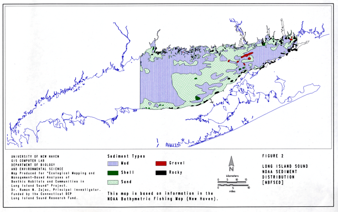
Figure 2. Distribution of sediment types in Long Island Sound given in the NOAA Bathymetric Fishing Map - New Haven. Areas of each sediment type are given in Table 1. This map is the NBFSED coverage in the Benthic GIS.

Figure 3.

Figure 4. Bulk sediment characteristics in Long Island Sound based on observations by Pellegrino and Hubbard (1983). The percentage of each type of sediment is given in Table 1. This is the BULKSED coverage in the benthic GIS. Sediment classifications shown on the map are as follows:

g - Gravel
gs - Gravel, Sand
gsh - Gravel, Shell
gssh - Gravel, Sand, Shell
m - Mud
mg - Mud, Gravel
ms - Muddy Sand
msgsh - Muddy sand, Gravel, Shell
msh - Mud, Shell
r - Rocky
s - Sand
sg - Sand, Gravel
sh - Shell
shs - Shell, Sand
sm - Sandy mud
smsh - Sandy mud, Shell
sr - Sand, Rocks
ssh - Sand, Shell

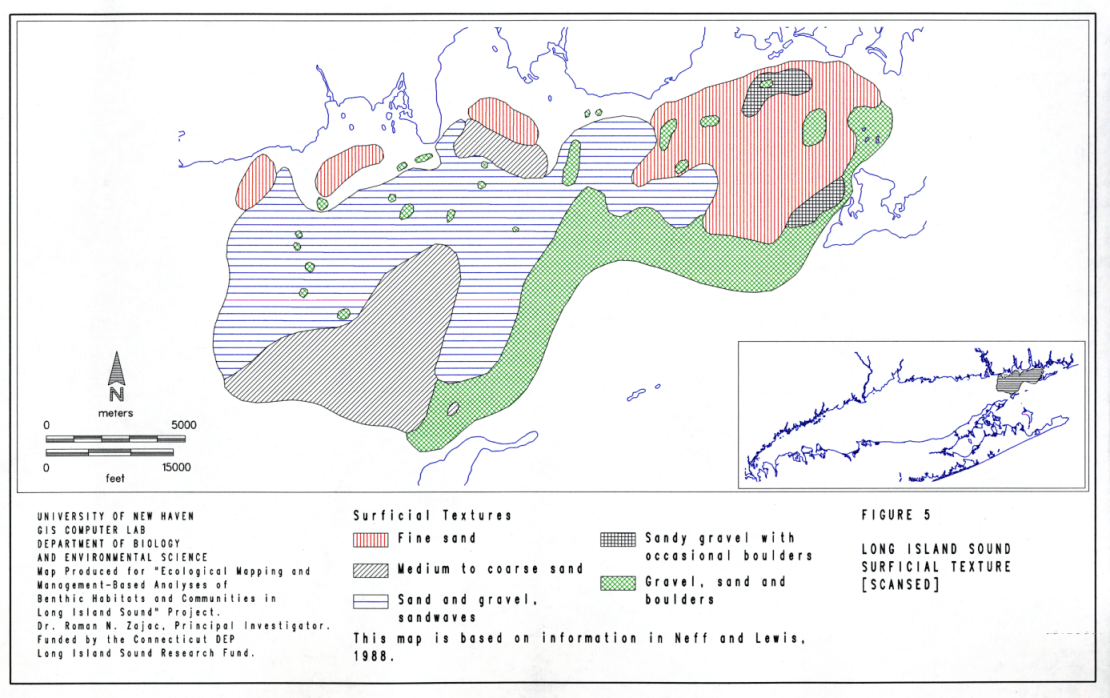
Figure 5. Surfice geological features, sediment texture and sediment types of the seafloor in the eastern portion of Long Island Sound based on interpretations of side scan images by Neff et al. (1988). Areas of each sediment type are given in Table 1. This is the SCANSED coverage in the Benthic GIS.

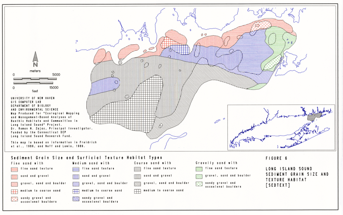
Figure 6. Benthic habitat map for the eastern portion of Long Island Sound. The map was developed by overlaying Figures 1 and 5 using GIS in order to indentify habitats based on the predominant sediment grain-size and surface texture features identified on side scan images. Seventeen habitat types were identified. The area of each habitat type is given in Table 1. This is the SEDTEXT coverage in the Benthic GIS.

Figure 7. General sequence of steps in the development of habitat maps for areas in Long Island Sound. SCANSED, LISSED, NBFSED, BULKSED and SEDTEXT refer to maps shown in Figures 5, 1, 2, 4 and 6, respectively. SCANMO1 refers to the side scan mosaic developed for the field site in the eastern portion of Long Island Sound (Lewis et al., this CD-ROM). Examples of other GIS coverages that can be used are given in Table 2.

Figure 8. Sampling stations for major offshore benthic surveys conducted in Long Island Sound. Locations are based on data provided in the studies cited on the figure. See Table 3 and text for further information on the surveys.

Figure 9.

Figure 10.

Figure 11. Model of soft-bottom community responses to disturbance / pollution gradients. Stage 1 represents early successional communities following disturbance or communities in polluted habitats. Stage 3 communities represent successional endpoints or communities in non-polluted habitats. Stage 2 are intermediate in both scenarios. See text for more details. The figure is reproduced from Rhoads and Germano (1982) and is based on models presented in Rhoads et al. (1978) and Pearson and Rosenberg (1978).

Figure 12. Distribution of molluscan assemblages in Fishers Island Sound based on data and analyses presented in Franz (1976). Each of the groups shown were determined based on multivariate analysis and are comprised of the numerically dominant species found in each cluster relative to the predominant sediment type found at the stations comprising each cluster.

Figure 13.

Figure 14. Spatial distribution of amphipod and polychaete assemblages in Fishers Island Sound based on data provided in Biernbaum (1974, 1979) and Swanson (1977). Assemblage types were determined via classification analysis (Figure 13). Mean abundances of species comprising each group are given in Table 7. Details of how the analysis was performed and assemblage characteristics are given in the text.

Figure 15. Spatial distribution of benthic species richness in Long Island Sound based on data provided in Pellegrino and Hubbard (1983). Richness is the number of species per 0.04 m² sample taken at each sampling point.

Figure 16. Spatial distribution of polychaete assemblages in Long Island Sound. Assemblages (denoted as A, B, C, etc. on the figure) were determined via multivariate clustering analysis of data provided in Pellegrino and Hubbard (1983). Further information on the analysis and the assemblage characteristics can be obtained from the author.

Figure 17. Spatial distribution of bivalve assemblages in Long Island Sound. Assemblages (denoted as A, B1, B2, etc. on the figure) were determined via multivariate clustering analysis of data provided in Pellegrino and Hubbard (1983). Further information on the analysis and the assemblage characteristics can be obtained from the author.

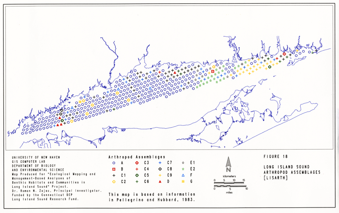
Figure 18. Spatial distribution of arthropod assemblages in Long Island Sound. Assemblages (denoted as A, B, C1, etc. on the figure) were determined via multivariate clustering analysis of data provided in Pellegrino and Hubbard (1983). Further information on the analysis and the assemblage characteristics can be obtained from the author.

Figure 19. Dendrogram showing the results of a classification (clustering) analysis of numerically dominant species in Long Island Sound based on data provided in Pellegrino and Hubbard (1983). Letters along the side of the dendrogram (A, B, C1, etc.) denote station clusters that were interpreted from the analysis and subsequently mapped (see Figure 20). The species composition of each cluster is given in Table 9.

Figure 20. Spatial distribution of benthic communities identified via clustering analysis of data provided in Pellegrino and Hubbard (1983). See Table 9 for group characteristics of each cluster. This map is the LISCOM coverage in the Benthic GIS.

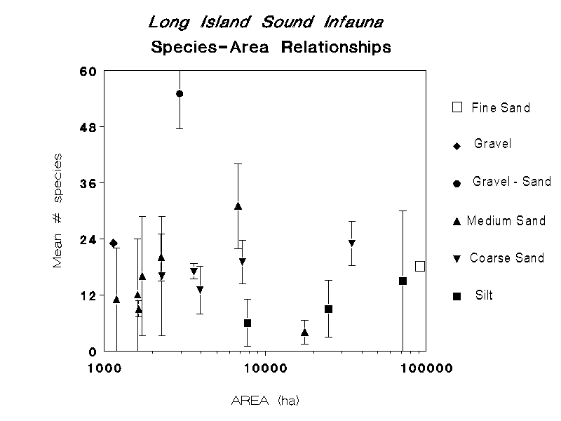
Figure 21. Mean number of species (" 1 SE) per 0.04 m2 in different sediment types in Long Island Sound. The analysis was done by grouping the sampling stations in the Pellegrino and Hubbard (1983) survey based on their bulk sediment characteristics (see Figure 4 and Table 1) and then calculating species richness for each sediment type. Sediment type designations are as follows:

g - Gravel
gs - Gravel, Sand
gsh - Gravel, Shell
gssh - Gravel, Sand, Shell
m - Mud
mg - Mud, Gravel
ms - Muddy Sand
msgsh - Muddy sand, Gravel, Shell
msh - Mud, Shell
s - Sand
sg - Sand, Gravel
sm - Sandy mud
smsh - Sandy mud, Shell
sr - Sand, Rocks
ssh - Sand, Shell
sh - Shell
shs - Shell, Sand
r - Rocky

Figure 22. Mean density of individuals (" 1 SE) per 0.04 m2 in different sediment types in Long Island Sound. The analysis was done by grouping the sampling stations in the Pellegrino and Hubbard (1983) survey based on their bulk sediment characteristics (see Figure 4 and Table 1) and then calculating density for each sediment type. Sediment type designations are as follows:

Figure 23. Relationship between patch area and the mean number of species per 0.04 m2. The patch area of different sediment types was determined using the LISSED coverage (Figure 1). Sampling stations from the Pellegrino and Hubbard (1983) survey (Figure 8) were grouped based on in which patch they occured and the mean number of species per sample was calculated for each patch.

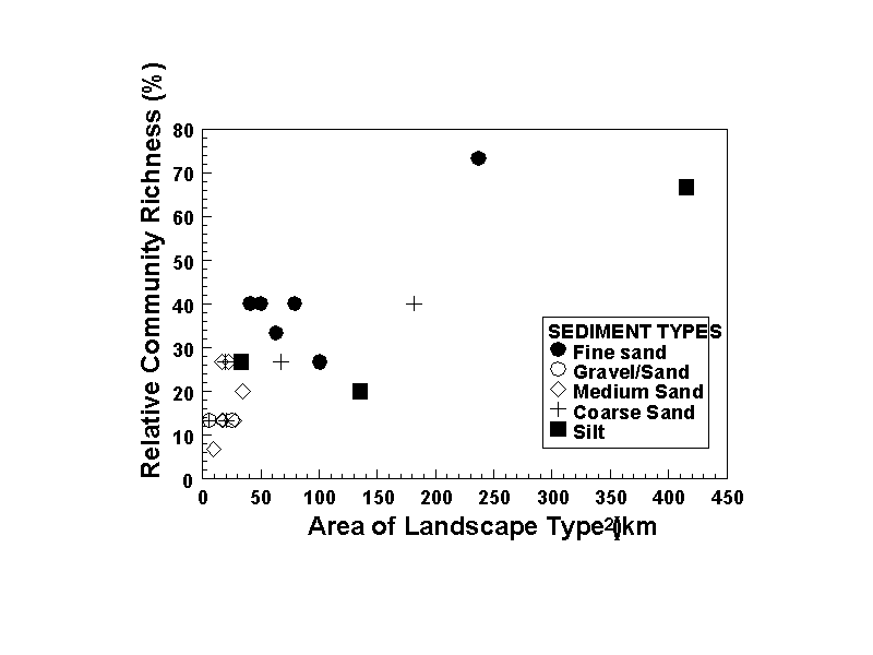
Figure 24. Relationship between landscape type area (i.e. patch area) and relative community richness. Landscape types are based on the large-scale sediment patches in Long Island Sound shown in the LISSED coverage (Figure 1). In this analysis, the area of each patch was calculated from a modified LISSED coverage in which the southern edge of each patch was defined by the southernmost extent of the sampling conducted by Pellegrino and Hubbard (1983). This roughly corresponds to the Connecticut - New York border through the long axis of the Sound. This was done in order to constarin the analysis only to the areas that were actually sampled. Also, in the LISSED coverage fine sand occurs as one continous patch (or GIS polygon) and for this analysis was broken down into several polygons. Relative community ricnhess is the percentage of community types in each patch out of all 15 possible types determined from multivariate analysis (Figures 19 and 20, Table 9).

Figure 25.

Table 1. Areas of each sediment type identified in Figures 1,2, 4, 5 and 6 (the GIS coverages) and discussed in the text.

Table 2. Listing of other GIS coverages that can be used to develop benthic habitat maps for Long Island Sound in conjunction with coverages presented in this report. The coverages developed as part of this project have also been given to the CT DEP.

Table 3. Survey studies conducted on soft-sediment community structure in Long Island Sound.

Table 4. Soft - sediment studies conducted in Long Island Sound which have centered on either dynamics of specific populations, responses to specific types of disturbances, sediment / organisms interactions or are syntheses of previous work. This list is only a sample of these types of studies; see also Lewis and Coffin (1985) or contact the CT DEP LIS Resource Center (Univ. CT Avery Point Campus, Groton, CT).

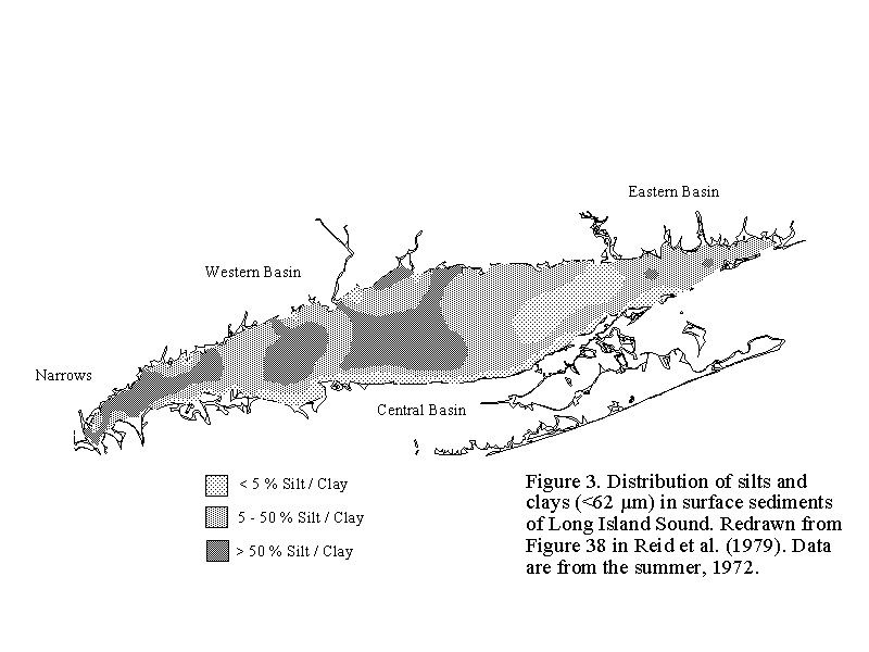
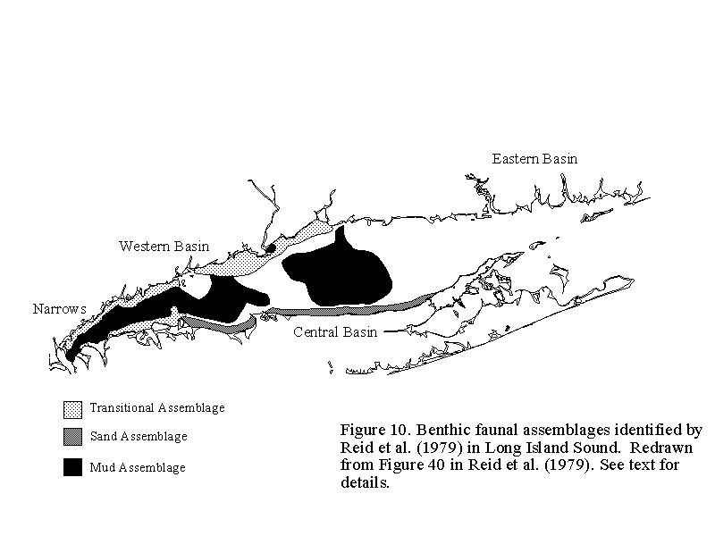
Table 5. Characteristics of the three faunal groups and their habitats recognized by Reid et al. (1979) via cluster analysis of 1972 samples. Shown are the mean densities per m² and coeffiecient of variation (in parentheses) of dominant infaunal species in 1972 and 1973 (based on data presented in Tables 4,5 and 6 in Reid et al. 1979) and for the muddy, deepwater group for 1975-1978 based on data presented in Table 3 in Reid (1979). Means are based on all samples in each group; means for total numbers of individuals and species are based on all species found at each station. See Figure 10 for the spatial distributions of each group.

Table 6. Ecological characteristics of Group I and Group III type species.

Table 7.

Table 8. Summary of benthic community characteristics in each of the geographical regions of Long Island Sound surveyed by Pellegrino and Hubbard (1983). B, bivalve; P, polychaete; A, arthropod. The number of species is the total number of species indentified in the region and the number of individuals in the mean abundance per 0.04 m2 sample.

Table 9.

Table 10. Results of one way analysis of variance (ANOVA) testing differences in species richness and total abundance among sediment types in Long Island Sound. All data are from Pellegrino and Hubbard (1983). Sediment categories are based on qualitative bulk sediment characteristics (Figure 4). Species richness and abundance are based on all species collected in a 0.04 m² sample at each sampling site.

[an error occurred while processing this directive]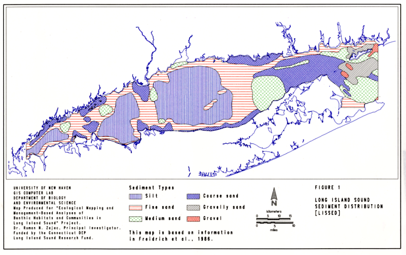