| |
Measuring Streamflow
The USGS began measuring streamflow in 1888 as part of studies
involving irrigation of public lands. Streamflow measurements are
made by direct or indirect methods. Most direct measurements are made
by sounding stream depths and measuring stream velocities with meters.
Low-flow streamflow measurements are made with wading rods and pygmy
meters (figs.
1, and
2). Most flood measurements are made using large meters and heavy
depth-sounding weights suspended from steel cables (fig.
3). Flood measurements usually are made from bridges (fig.
4) or boats, but years ago many flood measurements were made from
cars suspended from cables that traverse streams (fig.
5) or from equipment mounted on automobiles (fig.
6). Other direct measurements of streamflow are made by acoustic,
optical, or radar equipment and by injection of dyes. Many flood-peak
discharges are based on indirect measurements, which are made by applying
open-channel hydraulic principles to surveyed peak-stage profiles
along stream channels. Indirect measurements are used to compute peak
discharges in open channels or at bridges, culverts, dams, and other
hydraulic structures that constrict the peak water surface.
Streamflow-Gaging Stations
Streamflow generally cannot be continually sensed or recorded. The
objective in operating a streamflow-gaging station is to obtain
a continuous record of stage (water-surface elevation or gage
height) in the stream from which a continuous record of discharge
can be computed for the site. A continuous record of stage is obtained
by installing instruments that sense and record the stage in the
stream. Discharge measurements are made at various stages to define
the relation between stage and discharge and are made at periodic
intervals to verify the stage-discharge relation or define any change
in the relation due to changes in channel geometry. Weirs and dams
are constructed at some stations to stabilize the channel geometry
and thus the stage-discharge relation. The stage-discharge relation
is known as a rating curve. From the rating curve, a table of corresponding
stage and discharge values is developed for each streamflow-gaging
station and used to convert stage to discharge.
The first streamflow-gaging station was installed in 1889 on the
Rio Grande near Embudo, N. Mex. Streamflow stations from then until
about 1960 contained stilling wells on stream banks (fig.
7). A pipe from the well to the stream allowed the water level
in the well to be the same as that in the stream. A float in the
well was attached to a graphic recorder in the housing atop the
well, thus the gage height of the stream was continuously sensed
and recorded (fig.
8).
By about 1960, servo-control manometers and digital recorders were
being installed to replace the stilling wells (fig.
9). The gage height was sensed by measuring the water pressure
at the opening of a tube mounted near the bottom of the streambed
and extending to the gaging-station shelter. This equipment could
sense and record gage height from a shelter remote from the streambed.
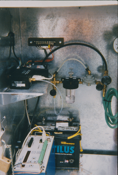
Beginning about 1995, pressure transducers and data loggers were
being installed (fig.
10). This equipment was smaller, less complicated, and more
reliable than the servo-control equipment. Modem and satellite transmitters
and antennas also were being installed (fig.
11) so that gage-height data could be transmitted, processed,
and presented in near-real time on the World Wide Web (Web).
Historical and near-real-time gage heights and discharges for Texas
streams are presented on the Web at tx.usgs.gov.
|
|
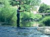
Figure 1
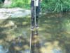
Figure 2
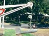
Figure 3
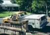
Figure 4
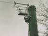
Figure 5

Figure 6
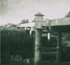
Figure 7

Figure 8

Figure 9

Figure 10

Figure 11
|
