U.S. Geological Survey OFR 2007-1397
2ETI, St. Petersburg, FL 33701.
Suggested citation: Robbins, L.L., Hansen, M.E., Raabe, E.A., Knorr, P.O., and Browne, J., 2007, Cartographic Production for the Florida Shelf Habitat (FLaSH) Map Study: Generation of Surface Grids, Contours, and KMZ files, U.S. Geological Survey, St Petersburg, FL , Open-File Report 2007-1397, 11 pages.
OFR 2007-1397 as a PDF document.
NOTE: PDF files may be viewed using free Adobe Reader freeware.
This report details the cartographic-production methods developed for files used in the Florida Shelf Habitat Mapping Project (FLaSH Map). FLaSH Map was initiated in 2006 to follow the goals set for the Coastal and Marine Geology National Benthic Habitat Studies in general, including mapping and characterizing benthic habitats at appropriate scales and resolutions, understanding geologic processes and environmental and human-induced change, developing a seafloor and habitat classification, extrapolating results from regional to national settings, developing prediction and modeling capabilities, publishing results as maps and reports; disseminating information through web sites; and managing data effectively, providing information and advice to management agencies, and facilitating intra- and interagency and international collaboration on benthic habitat research. A broad goal for the project is to provide the public with data through user-friendly avenues.
The U.S. Geological Survey (USGS) sponsored a workshop in partnership with the Florida Department of Environmental Protection and the Southeast Regional Partnership for Planning and Sustainability (SERPPAS) in January 2007 to discuss the mapping priorities for the state. Workshop participants identified high-priority topics and areas for mapping projects (FDEP, 2007). A top-priority topic for researchers and agencies was bathymetry coverage at scales appropriate to habitat and resource evaluation.
The files described here are utilized on the FLaSH Map website (FLaSH, 2007), and are viewable in ©Google Earth. The Florida shelf bathymetry data are provided in three formats with this release. All of the data maps are produced entirely through digital means. This Open-File Report describes the techniques developed and/or adopted by the FLaSH Map Team at the USGS Florida Integrated Science Center (FISC) for Coastal and Watershed Studies in St. Petersburg, FL. These methods were found to be effective for this project, but this does not eliminate the possibility that other methods are available or more effective than those utilized.
The techniques described were used to create three different map types projected in FLaSH website, ©Google Earth, and as Geographic Information System (GIS) data files for end-users. Surface grids and contour lines were created from National Oceanic and Atmospheric Association (NOAA) bathymetric (x,y,z) data using ArcMap, part of ArcGIS by Environmental Systems Research Institute, Inc. (ESRI). Next, the files were converted to Keyhole Markup Language (KML) or zipped KML (KMZ) files. USGS Geological LOng-Range Inclined Asdic (GLORIA) data in Geo-referenced Tagged Image File Format (GeoTIFF) file format were processed to create KMZ files for ©Google Earth.
ArcMAP is a general-purpose mapping system typically used for map creation and geographic analysis. Within the ArcMap application, a raster surface model is generated in the form of a rectilinear grid, a two-dimensional array of depth (z) values. The ArcMap raster grid is used for producing contour lines, profile maps, calculating volumetric data, and for grid-to-grid comparison.
The complete suite of bathymetric data utilized for FLaSH Map Project is compiled from many different sources, including data from NOAA and more high-resolution data acquired by the USGS and State and other Federal agencies. This report describes the process of gridding for NOAA bathymetric data and the sequential process that allowed refinement of the final product.
NOAA bathymetric digital sounding data were downloaded from the NOAA Hydro Search Criteria Selection Website (NOAA, 2007) as four tiles encompassing the Florida shelf. The first dataset was incomplete for some coastal areas and was supplemented by harbor and approach maps from the National Geospatial-Intelligence Agency Digital Nautical Chart® Website (NGA, 2007).
Unprocessed bathymetric data consist of a geographic coordinate (x, y) and a depth value (z). Depth values (z) are positive numbers. The available NOAA data were imported into ArcGIS as a series of point layers, formatted, and merged into one ArcGIS vector-point layer. Sounding points (soundp) were extracted from the NGA data, imported, and merged into the existing point layer. Obvious outlier points were removed.
Grid nodes, the intersections or corners of the grid cells, extend from the origin of the grid, lower left corner, to the east and north. Specific grid cell spacing and grid cell placement were used for each unique dataset. Specific spacing and placement parameters are vital to processing because during gridding and later grid editing, grid node positions must remain stationery in order to compare grids and contours. The outer dimensions of each grid are multiples of 100 m. The merged point layer was interpolated into a raster grid, a two-dimensional array of cells, using the inverse distance-weighted interpolation method with a variable search radius incorporating the nearest six points.
Three errors generally found in the grid include bulls-eyes, data distribution distortions, and negative contours crossing marine features. These features were edited through point deletion. In general, such edits were minimal.
The data points were acquired either directly from NOAA or through derived products. The data (z values) were not corrected to a specific vertical datum; however, all sounding data were reduced to Mean Lower Low Water (MLLW). NOAA vertical accuracy standards vary by depth; shallower readings are more accurate than deeper readings. For example, at 1 m the acceptable error is 0.5 m, at 100 m the acceptable error is 1.4 m, and at 1000 m the acceptable error is 23.0 m. The points that make up the point shapefile were gathered at different times and by different methods. The contour and grid layers were derived from the point shapefile, and as such, these products should not be used for navigation. The bathymetry contained in the contour and grid products is representative, not authoritative. Table 1 represents a general guide to vertical accuracy.
|
Error
(meters) |
Depth
(meters) |
|
0.500169 |
1 |
|
0.596343 |
25 |
|
0.820061 |
50 |
|
1.09573 |
75 |
|
2.507987 |
100 |
|
3.043949 |
125 |
|
3.592005 |
150 |
|
4.147364 |
175 |
|
4.707441 |
200 |
|
5.836309 |
250 |
|
11.5434 |
500 |
|
17.27896 |
750 |
|
23.02173 |
1000 |
|
46.01087 |
2000 |
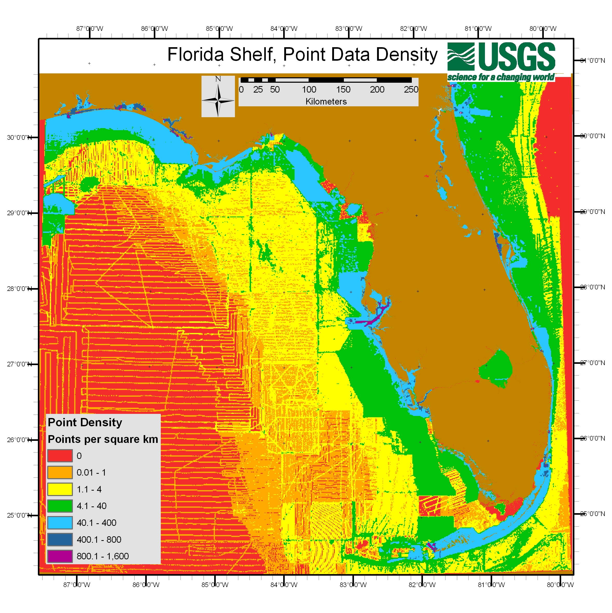
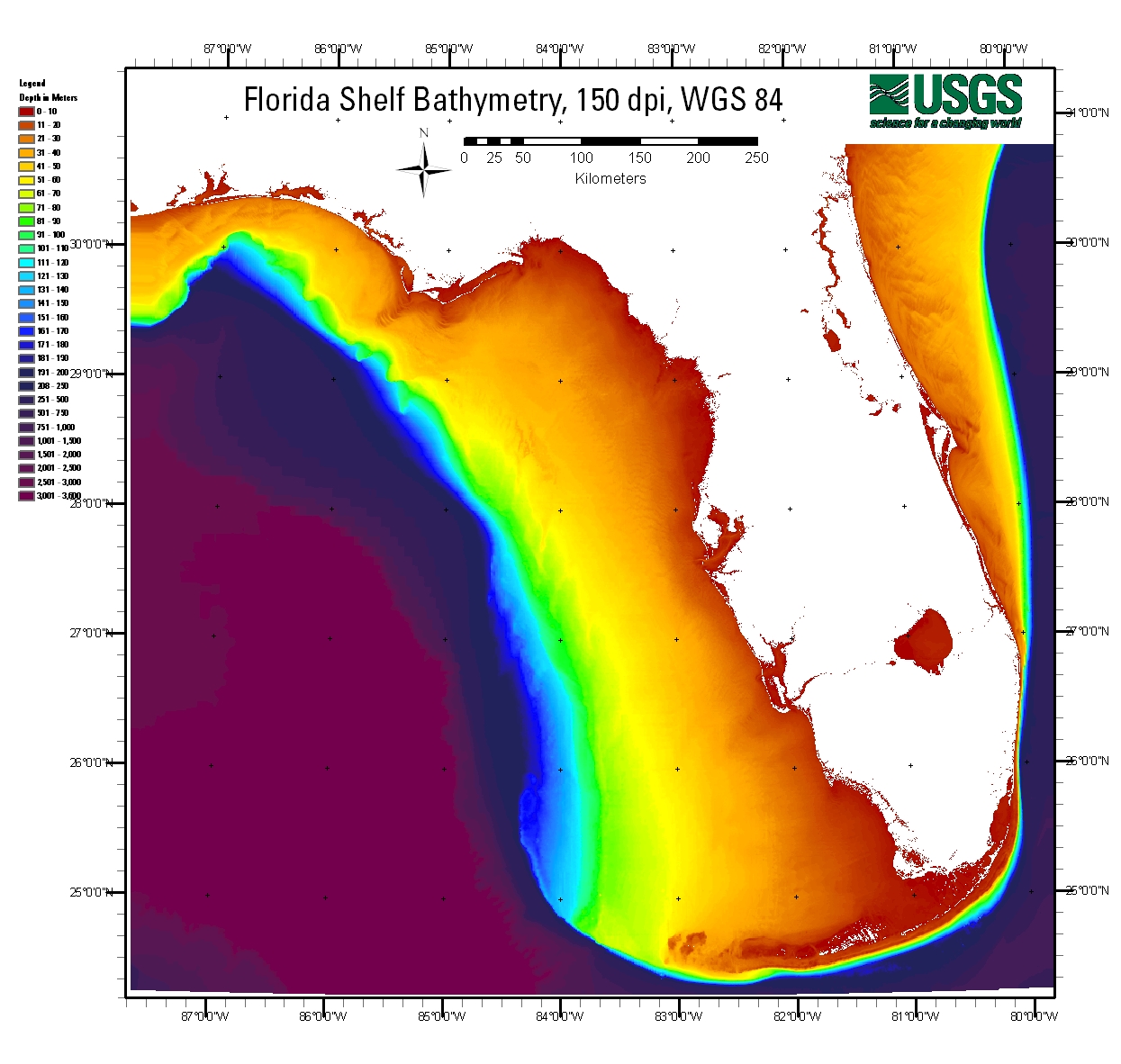
Bathymetric data points are often sparsely spaced in deeper water and offshore regions (Figure 1a). This type of data distribution presents problems when using a fine grid spacing (10 m x 10 m), because contour lines will be falsely distorted due to the data spacing. However, a disadvantage of coarse grids (1000 m x 1000 m) is that near the water/land interface, bathymetric contours will often erroneously cross over land features. Because neither grid resolution is appropriate in both the nearshore and offshore areas, the final grid spacing of 50 m was a compromise of the best parts of both grids. Depths are given as positive values in meters (Figure 1b).
The inverse distance-weighted interpolation method used to create the grid layer is a conservative technique that does not extrapolate beyond the minimum and maximum input values. Therefore, the depth at any specific point must fall within the range of the minimum and maximum values of the nearest six points. Thus, the grids are accurate but not precise. The interpolated products are a likely representation of bathymetry and have not been field-verified; they should not be used for navigation. Because the precision of the final products is a function of the point density, a coarser-resolution grid can be interpolated from a subset of the point layer to reflect sparser data conditions accurately when necessary.
After processing, all bathymetric data were projected to WGS 84 and Florida Albers NAD83 HARN using ArcGIS data-management projection utilities. The study area was subdivided into 36 tiles to allow conversion to KML format without loss of detail.
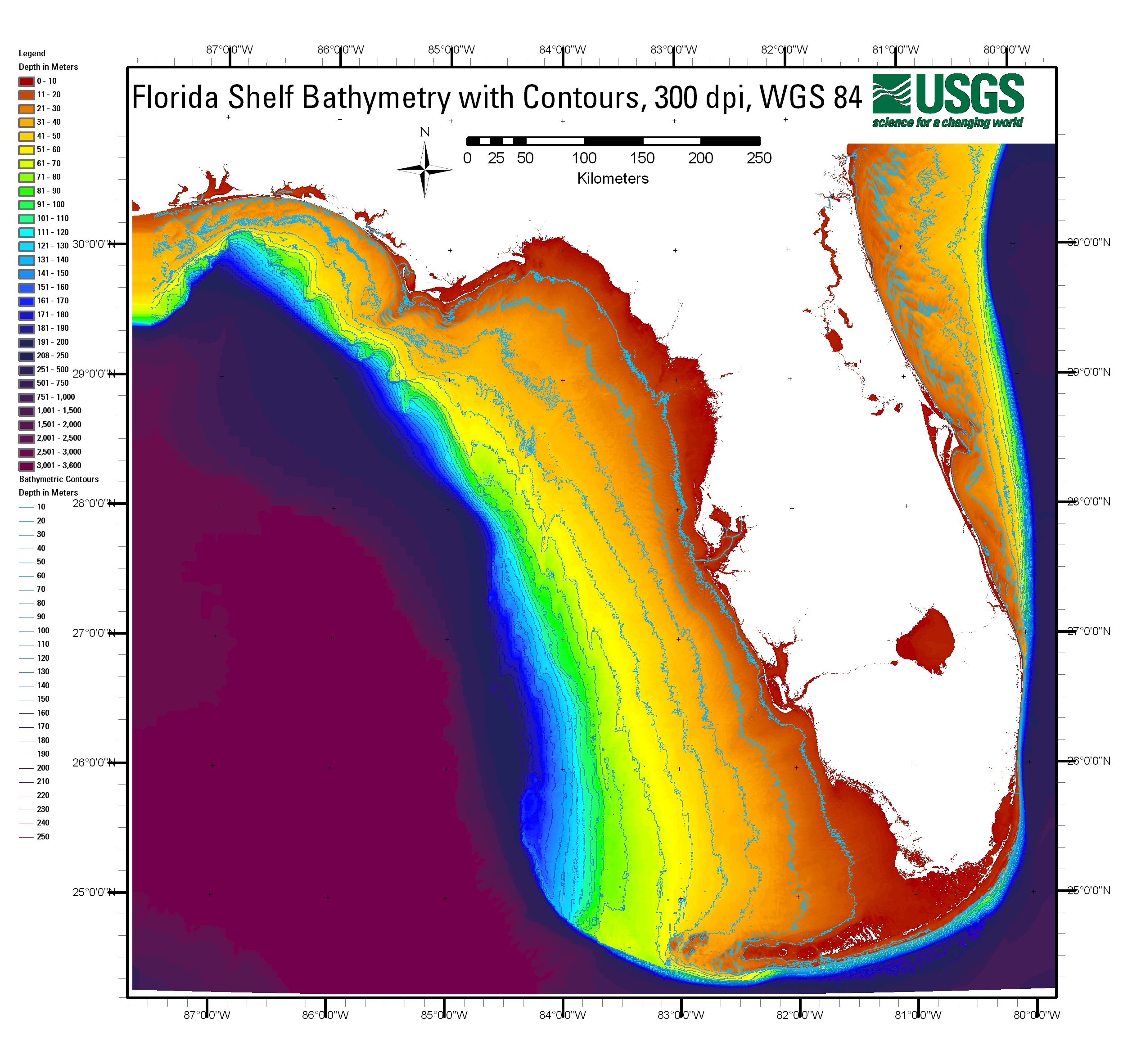
Contours were created at 10-m intervals in ArcMap using ArcMap 3D Analyst Raster Surface Contour routine (Figure 1c). Bathymetric data for the Florida shelf was prepared in three formats: point, grid, and contour (Table 2).
|
Layer |
Data Format |
Data Type |
Size |
Miscellaneous |
|
FlashPoint |
Vector |
ArcGIS Point |
721.35 MB |
Depths to 0.1 m |
|
Flashgrid50 |
Raster |
ESRI Grid |
873.99 MB |
50-m pixel |
|
FlashContour10 |
Vector |
ArcGIS Polyline |
2.71 MB |
10-m contour interval |
Figure 1. Florida shelf bathymetry showing (a) data points, (b) raster data, and (c) 10-m contours
Click on images to open in new window; click on newly opened window to zoom in.
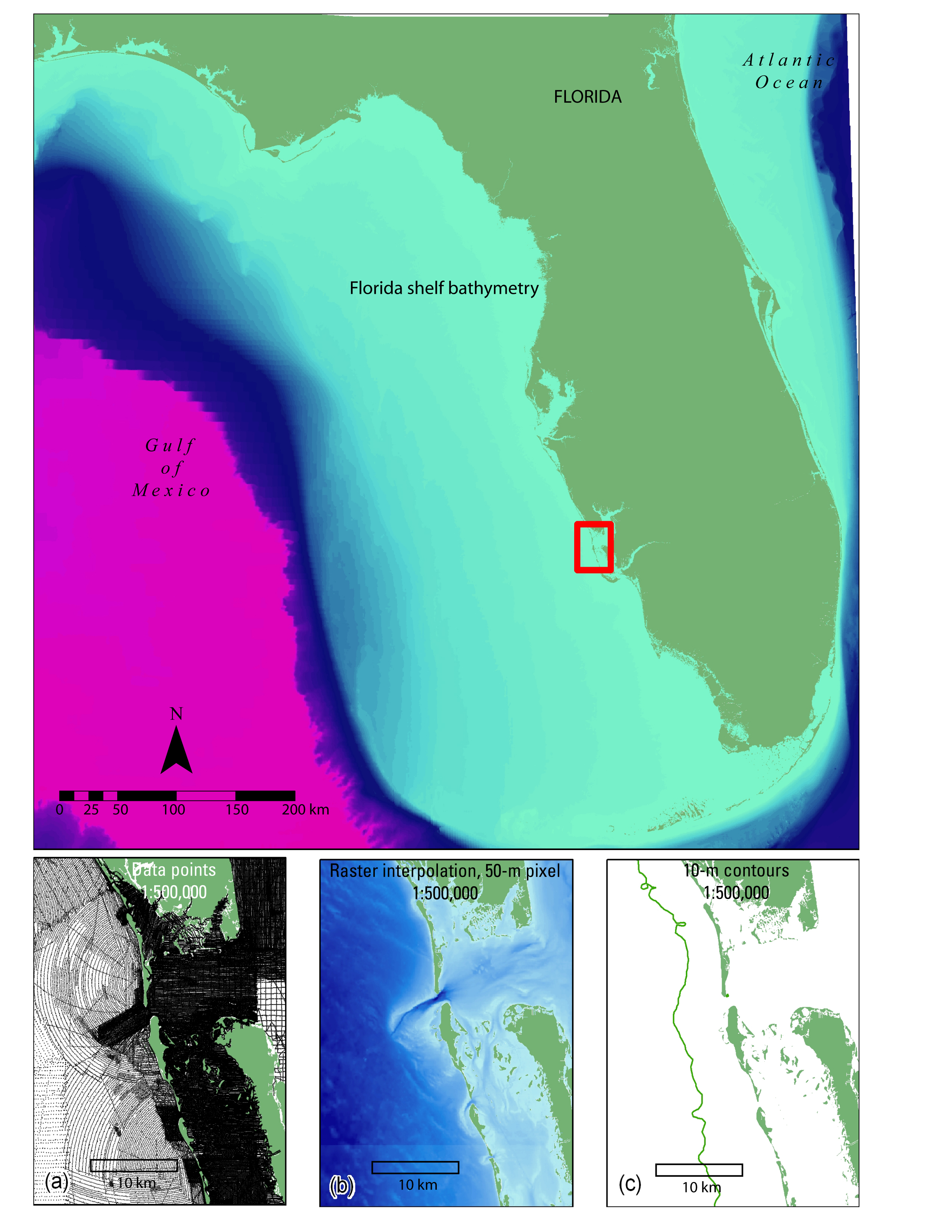
Links to larger images of Florida shelf data point density, 50-meter bathymetry grid, and 10-m contours.
Compressed (zipped) Keyhole Markup files were created from the combined gridded raster data and hillshade grids using the ArcMap Arc2Earth utility. KMZ file format is the standard data-file format for displaying images in ©Google Earth software. The "Base Image Path" was set to "images" in order to comply with the KMZ standard, and these images were manually put into the images folder. The folder was opened by changing the KMZ extension to ZIP, data extracted to another folder, and the images were cut and pasted into "images" folder. This folder was then rezipped and the extension changed back to KMZ.
The GLORIA data consist of 250-m-resolution sidescan-sonar imagery of the Gulf of Mexico seafloor (Gardner et al., 1996). An excellent description of the data and their geologic interpretation were published by Paskevich (2000). GLORIA data were downloaded from the USGS GLORIA mapping program website (GLORIA, 2007) and were imported into ArcMap. Specifically, data from USGS Open-File Report 00-019 (Paskevich, 2000) were used.
The GIS-ready data did not require any additional cleanup, formatting, renaming of fields, or other "data work" to convert the data to KMZ files. We utilized the original GeoTIFF files for the maps that are projected in FLaSH website (FLaSH, 2007) and ©Google Earth.
All GLORIA GeoTIFF files were projected according to the original dataset (NAD 1927 Albers Conical Equal Area projection; GLORIA, 1988; GLORIA, 1996; Paskevich, 1996). The composite image was downloaded (Paskevich, 2000) using the ArcGIS tool, "Mosaic to Raster." Sixteen mosaics and one low-resolution composite raster were converted into a single raster image. The "Mosaic Method" and the list of data were adjusted so the high-resolution mosaics would always be favored over the composite. The data were exported from ArcGIS to a single ©Google Earth compatible file in KMZ format using Arc2Earth software (Arc2Earth, 2007). We then set the "Base Image Folder" to "Images" in order to create KMZ standard-compliant files.
Sediment maps for FLaSH Map were created from USGS Data Series 146 (Buczkowski et al., 2006). This database includes sediment data from the Gulf of Mexico (version 1.0) and extends from the Florida Keys to Texas/Mexico border, including major estuaries such as Pensacola Bay and Tampa Bay. Within usSEABED, two types of sediment data are available, including point data (extracted) and descriptive data (parsed). For the purpose of the maps created for the FLaSH website, only extracted size data (in phi) were used.
ESRI ArcGIS software was used to contour the sediment data. The ArcGIS Import Table Wizard was used to import usSEABED data in order to add text files to the database. All cells in the database with an entry of -99 were replaced with a value of NULL, indicating missing or unknown data, and the entire geodatabase was added to ArcGIS. Raster data were created by displaying XY data and running Natural Neighbor and IDW tools within ArcMap. Within the IDW tool, the search radius was set to Variable and Number of Points was set to 4. The Maximum Distance was left blank. Using Angle-Output Map Algebra tool (SETNULL( 1-ISNULL(
Using Arc2Earth, the single raster data were exported to KMZ files by setting Base Image Folder to images in order to meet KMZ compliancy standards. Legends were modified to aggregate values into visually distinct categories and were changed to include the name of sediment being considered. Data density overlay was also added so that the viewer can qualitatively determine how dense the sediment data were in an area.
The goal of the Florida Shelf Habitat Mapping Project is to provide the broadest user-base with the data, which can be visualized through the most user-friendly means. Visualization of bathymetric, sediment, and sidescan data from the Florida shelf required a combination of processing techniques. These methods are reported here, and the series of maps can be visualized on the FLaSH Map website (http://coastal.er.usgs.gov/flash), in GIS format where available, and through ©Google Earth (http://earth.google.com/).
We thank Arnell Harrison, Nancy Dewitt, and Beau Suthard (Coastal Planning & Engineering, Inc.) for their insightful comments.
Arc2Earth, 2007, Arc2Earth software: http://www.arc2earth.com/
Buczkowski,
B.J., Reid, J.A., Jenkins, C.J., Reid, J.M., Williams,
S.J., and Flocks, J.G., 2006, usSEABED: Gulf of
Mexico and Caribbean (
FDEP, 2007, Florida Regional Marine Mapping website, http://www.dep.state.fl.us/marinemapping/
FLaSH, 2007, Florida Shelf Habitat (FLaSH) Map Website: http://coastal.er.usgs.gov/flash
GLORIA Sidescan
Sonar Field Data and Navigation Data Collected in the Gulf of Mexico During R/V Farnella
Cruises in 1982 and 1985: 1996,
GLORIA, 1988, GLORIA Data:
GLORIA, 2007, GLORIA mapping program website: http://coastalmap.marine.usgs.gov/gloria/
NGA, 2007: National Geospatial-Intelligence Agency Digital Nautical Chart® Website: http://www.nga.mil/portal/site/dnc/index.jsp?front_door=true
NOAA, 2007: NOAA's Hydro Search Criteria Selection Website: http://www.ngdc.noaa.gov/mgg/gdas/ims/hyd_cri.html
Paskevich, V.F., 1996, Digital Mosaics of the GLORIA Sidescan Sonar Data of the Gulf of Mexico, U.S. Geological Survey Open-File Report 96-657, 1 CD-ROM.
Paskevich, V.F., 2000, Gulf of Mexico GLORIA Sidescan Sonar Geologic Interpretation: ArcView Data Coverages, U.S. Geological Survey Open-File Report 00-019 https://pubs.usgs.gov/of/2000/of00-019/