U.S. Geological Survey Open-File Report 2012-1038
MethodsPlant Identification WorkshopTo improve and standardize knowledge of the local tidal wetland flora for USGS and EPA personnel, a 1-day workshop taught by Laura Brophy was held in May 2010. USGS and EPA staff visited three tidal wetlands in the Yaquina estuary, representing a range of salinity regimes. Workshop training provided the foundation for subsequent large-scale estuarine vegetation surveys conducted by the USGS and EPA during 2010 in four coastal estuaries in Oregon. Data Processing StepsIn February 2010, NWI shapefiles for the Yaquina drainage basin were downloaded from the NWI website (U.S. Fish and Wildlife Service, 2010) and merged into one data layer by EPA. In April 2010, NWI shapefiles for the Alsea Bay drainage basin were downloaded from the NWI website and merged into one data layer by Green Point Consulting. Metadata for these NWI data list the date of the source imagery as "1977 to present". The NWI data layers were then processed in the following ways:
LiDAR AnalysisLiDAR-derived elevations were obtained from the "bare earth" digital elevation model developed for the Oregon LiDAR Consortium by Watershed Sciences, Inc. (Watershed Sciences, Inc., 2009; Oregon Department of Geology and Mineral Industries, 2012). Standard (not water-penetrating) airborne LiDAR equipment was used. Data acquisition was not timed for low tide, but for this study area, all ground surfaces critical to the analysis (that is, surfaces above Mean Higher High Water) were above water in the LiDAR data. The vertical accuracy of the LiDAR data was 0.11 ft, determined through Real Time Kinematic ground survey on road surfaces, compared to the closest laser point (Watershed Sciences, Inc., 2009). Average laser pulse density was 0.80 per ft2 (Watershed Sciences, Inc., 2009). The LiDAR analysis focused on the upper limit of tidal influence, since NWI mapping of habitat classes lower in the tidal range (that is, low marsh, mud flat, aquatic bed) appeared to be accurate. To determine the upper limit of tidal influence, LiDAR derived elevations were analyzed to determine the percentage of each NWI polygon that occurred within three elevation zones (table 2). Table 2. Elevation zones used for LiDAR analysis (elevations in feet (ft) NAVD88), Yaquina and Alsea estuaries, Oregon.
These elevation ranges were developed by reviewing tidal datums for the two estuaries (table 3) and comparing those datums to field knowledge of the Yaquina and Alsea estuaries gained during multiple projects (Brophy, 1999, 2003, 2004, 2006, 2009; Brophy and Christy, 2008, 2009, 2010; Brophy and others, 2011). Table 3. Tidal datums for the Yaquina and Alsea estuaries, Oregon. [MLLW= Mean Lower Low Water; MHHW= Mean Higher High Water; HMT=Highest Measured Tide]
1 Where a range of values is provided, the range includes all locations within the specified estuary, as provided by the source at left. The entry "n/a" indicates the value was not provided relative to the NAVD88 geodetic datum. 2 Hamilton (1984) provides elevations relative to the NGVD29 or NGVD29(47) datum. Elevations relative to the NAVD88 datum were determined by applying the elevation adjustments at http://www.ngs.noaa.gov/cgi-bin/VERTCON/vert_con.prl The elevation zones defined in table 2 were deliberately broad to reflect the range of published values in table 3 and the limited number of field studies of inundation regimes in the Yaquina and Alsea estuaries. Because this analysis focused on the upper limits of tidal influence, the elevation zones in table 2 did not subdivide elevations below Mean Higher High Water (MHHW). The elevation zones in table 2 extended well above MHHW for several reasons: First, studies have documented that brackish high marsh and brackish to freshwater tidal swamps (scrub-shrub and forested tidal wetlands) in Oregon generally are found at elevations well above MHHW. For example, at the Bandon Marsh National Wildlife Refuge in the Coquille River estuary, the elevation of a forested tidal wetland in the lower estuary (bay fringe) was 8.2 ft NAVD88, which is 1.2 ft above MHHW (Brophy and van de Wetering, 2012). At a strongly fluvial site in the Siuslaw River estuary, the elevation of a freshwater tidal wetland was 8.6 ft NAVD88 (1.5 ft above MHHW); model simulations showed that this site is tidally inundated about 2 percent of the time during typical months of December and January (Brophy, 2009). Second, inundation at these high tidal wetlands is the product of both tidal forces and river flows (fluvial forces). As indicated in table 2, inundation in elevation zone 2 is primarily seasonal. Combined tidal and fluvial inundation occurs more often in winter when river flows are high (Brophy, 2009; Brophy and others, 2011). The contribution of river flow to tidal amplitude is particularly strong in the middle and upper estuary where river valleys are more confined (Brophy, 2009; Brophy and others, 2011; Huang and others, 2011). Model simulations have not yet fully explored the highest potential elevations of this combined fluvial-tidal inundation. Finally, dense vegetation may interfere with the LiDAR signal, resulting in "bare earth" elevations that are higher than the actual ground surface elevation (Gopfert and Heipke, 2006). This effect is particularly pronounced in the freshwater tidal zone (upper estuary) in dense monotypic stands of slough sedge (Carex obnupta) and reed canarygrass (Phalaris arundinacea) (Brophy and van de Wetering, 2012). Land surfaces within the lowest elevation zone (<8 ft for the Alsea estuary, <9 ft for the Yaquina) are clearly tidal wetlands, based on information from previous studies (Brophy, 2009; Brophy and others, 2011), tidal datums (table 3), and data provided by EPA. For example, EPA analysis of National Oceanic and Atmospheric Administration (NOAA) tidal height records from 2004 to 2008 show that in the lower Yaquina estuary, wetlands at 9.0 ft NAVD88 (1.4 ft above MHHW) are submerged by tidal waters at least once per month year-round (J. Stecher and C. Janousek, unpub, data, 2011). The next elevation range (8–11 ft for the Alsea, 9–11 ft for the Yaquina) includes land surfaces likely to experience tidal inundation during winter, or in spring and fall during spring tide cycles or high river flows. The top elevation range (11–13 ft) covers the range of NOAA values for HMT (Highest Measured Tide) recorded at NOAA’s local tidal stations and therefore includes potential waters of the State, as either Tidal Waters (OAR 141–085–0515(2)) or wetlands (OAR 141–085–0510(97)), as described in Oregon administrative rules. However, this higher range was not used in our final analysis, as tidal wetlands in the Yaquina and Alsea estuaries generally occurred below this elevation range. To determine the percentage of each NWI polygon that occurred within the elevation zones in table 2, the NWI data were first reprojected to Oregon Statewide Lambert NAD83 HARN to match the projection of the LiDAR-derived elevation datasets. The LiDAR raster dataset (DEM) for each estuary was then reclassified using Environmental Systems Research Institute (ESRI) Spatial Analyst to create two new discrete raster datasets: Dataset 1: Value of 1 = <9 ft (Yaquina) or <8 ft (Alsea), value of 0 = other elevation; Dataset 2: Value of 1 = 9–11 ft NAVD88 (Yaquina) or 8–11 ft (Alsea), value of 0 = other elevation. The NWI polygons were then intersected with these two discrete raster datasets using the "Isectpolyrst" command with proportion = TRUE in the ArcMap Geospatial Modeling Environment. This created a new attribute in the NWI layer showing the percent of each NWI polygon with a value of 1 or 0 for each of the two elevation classes (<8 ft versus 8–11ft for the Alsea; <9 ft versus 9–11 ft for the Yaquina). NWI polygons with more than 25 percent of their area in these two elevation zones were compared to aerial photographs, field knowledge of the estuaries, and data from other studies (Brophy, 2003, 2004, 2007b, 2007c, 2009; Brophy and Christy, 2008, 2009; Brophy and others, 2011). The 25 percent threshold was based on these studies and data from other Oregon estuaries (Brophy and van de Wetering, 2012), and allowed for potential vegetation interference with the LiDAR signal as well as the fluvial contribution to water levels previously described. NWI polygons, which were considered very likely to be current or former tidal wetlands (based on aerial photograph interpretation, field knowledge, and other data), were selected and the appropriate Cowardin et al. classification was assigned (see section, "Wetland Classification"). The selected NWI polygons were then merged (Editor/Merge tool in ESRI ArcMap) to form the Prioritization Sites identified in the 1999 Yaquina and Alsea River Basins Estuarine Wetland Site Prioritization (Brophy, 2009) (see section, "Creation of GIS Data for 1999 Tidal Wetland Prioritization"). For extensive tide gated lands like Boone Slough, Nute Slough, Depot Slough, and Olalla Slough in the Yaquina estuary, few visual indicators remain of former tidal status. Substantial portions of these tide gated lands are within the <9 ft and 9–11 ft elevation zones, but are classified in the NWI as upland; however, these were very likely tidal wetlands prior to construction of the tidal flow barriers. A separate procedure to map these likely former tidal wetlands was developed to assist planning for future restoration projects (see section, "Likely Former Tidal Wetlands Classified as Upland in the NWI"). As in the 1999 prioritization (Brophy, 1999), lands
that have been filled and converted to developed uses were excluded from
this study, even if they were within tidal range. Examples include the
former log storage yard at the Siletz Tribes mill just downstream of Mill
Creek, on the northern bank of the Yaquina River, and industrial lands
on the banks of the Yaquina in the city of Toledo. Wetland ClassificationExpert knowledge of the Yaquina and Alsea estuaries, LiDAR-derived elevations, salinity data provided by EPA, and recent aerial photographs were used to determine the correct Cowardin et al. system, subsystem, class, hydrologic modifiers, and special modifiers for each NWI polygon identified as a tidal wetland using the methods described in the "LiDAR Analysis" Section. For consistency, these revisions followed the same definitions of wetland systems, subsystems, and classes used in the NWI (Cowardin et al. 1979). The elevation zones in table 1 were not used to classify the wetlands; they were used only for the previously described LiDAR analysis. The highest-resolution aerial photographs available
at the time of this study were color infrared photographs acquired jointly
by Department of Land Conservation and Development (DLCD) and EPA during
2004–06 (Oregon Department of Land Conservation and Development and others,
2007a, 2007b). These images had 0.25 m ground pixel resolution. The DLCD—EPA
imagery was supplemented by 2005 true color NAIP imagery (digital ortho
quarter-quads, 0.5 m ground pixel resolution). Photograph interpretation
was used to identify tidal channels, brackish versus freshwater vegetation,
topographic transitions, developed lands, dikes, restrictive culverts,
and tide gates, and other features that helped distinguish between tidal
wetlands and nontidal wetlands or uplands, and to provide other information
needed for wetland classification. Recommended classifications also drew
on other field studies of tidal wetlands in the Yaquina, Alsea, and other
Oregon estuaries (Brophy, 2003, 2004, 2007b, 2007c, 2009, 2012; Brophy
and Christy, 2008, 2009, 2010; Brophy and others, 2011), and salinity
data provided by EPA (C. Brown and C. Janousek, written commun, 2011). Estuarine versus Palustrine System (salinity regime)Wetlands with salinity equal to or greater than 0.5 (originating from marine salts) during low flow (summer and early fall) are classified in the Cowardin et al. system as estuarine wetlands (Cowardin et al. 1979). Tidal wetlands with salinities less than 0.5 (freshwater tidal wetlands) are classified as palustrine wetlands, and are assigned a "water regime modifier" to indicate tidal influence. Cheryl Brown of EPA provided a shapefile containing salinity data for the Yaquina estuary originating from many sources (more than 8,000 data points originating from EPA and the Oregon Department of Environmental Quality). Almost all measurements were on the main stem river, but sampling depth was variable (Cheryl Brown, written commun., 2011). Despite the NWI’s classification of tidal wetlands as palustrine upstream of river mile 14, these data showed late summer and early fall salinities in the range of 5–10 as far upstream as river mile 19.5, near the upstream limit of tidal wetlands in the estuary. Therefore, only very limited areas were classified as palustrine, tidally influenced wetlands. Additional data from upper Poole Slough on the Yaquina likewise revealed that other wetlands designated as palustrine tidal in the NWI are actually brackish habitats (C. Janousek and C. Folger, unpub. data, 2011). For the Alsea estuary, data from previous field studies (Brophy, 2003, 2006; Brophy and Christy, 2008, 2009, 2010) were used to determine which wetlands should be classified in the estuarine system versus the palustrine system. Field observations of vegetation were the primary means for this classification; dominance by brackish-tolerant species (based on field knowledge and Adamus, 2005) indicated wetlands that should be placed in the estuarine system. Salinity in a tidal wetland may differ from salinity in the adjacent tidal water body. For example, a forested tidal wetland near the hillslope base may have much lower salinity than the nearby tidal river because of freshwater drainage from the nearby uplands (Brophy, 2009; Brophy and van de Wetering, 2012). Where specific field data were not available, the aerial photographs (previously described) were used to help determine estuarine versus palustrine classification. Reed canarygrass (Phalaris arundinacea) (fig. A14) and red alder (Alnus rubra) (figs. A15–A16) are two species that are identifiable in aerial photographs and do not tolerate much salinity, based on our field experience and Adamus (2005). Aerial photographs were used to identify tidal wetlands that were dominated by these species, and these areas were classified as tidally influenced palustrine wetlands. Cowardin et al. (1979) Classification ModifiersWater regime (hydrologic) modifiers and special modifiers were included in our recommended Cowardin et al. classifications. Although the mapping standard used by the NWI does not require special modifiers for estuarine habitats (Federal Geographic Data Committee, 2009), the special modifiers we have provided in our mapping contain crucial information and should therefore be retained. Modifiers were used according to the definitions provided in Cowardin et al. (1979). Water Regime ModifiersWhen the Cowardin et al. classification is applied to Oregon estuaries, low salt marsh generally is assigned the "N" modifier, which is defined as "regularly flooded" ("tidal water alternately floods and exposes the land surface at least once daily") (Cowardin et al. 1979, p. 21), and high estuarine marsh is generally assigned the "P" modifier, which is defined as "irregularly flooded" ("tidal water floods the land surface less often than daily") (Cowardin et al. 1979, p. 21). In general, the water regime modifiers for wetlands already classified as estuarine in the NWI were not revised, because they were fairly accurate. However, "irregularly flooded" is not an accurate description of the high marsh inundation regime. Field measurements and model simulations indicate that high marsh is in fact regularly flooded, although much less often than low marsh. The typical pattern is inundation during higher high tides on spring tide cycles, once or twice a month (Brophy, 2009; Brophy and others, 2011). For NWI polygons that were classified as palustrine but the correct classification was estuarine (based on salinity data, as previously described), the "N" and "P" modifiers were applied as appropriate, based on elevation and our knowledge of the specific location. Estuarine scrub-shrub and estuarine forested wetlands (E2SS and E2FO) were assigned the "P" modifier, because in our study area these wetland types generally do not flood daily. For tidally influenced palustrine wetlands, the Cowardin et al. classification offers the same hydrologic regime modifiers used in nontidal systems, but with the word "tidal" added: R = seasonally flooded (tidal), S = temporarily flooded (tidal), T = semipermanently flooded (tidal), and V = permanently flooded (tidal). These modifiers are not well-suited to the observed flooding regimes in freshwater tidal wetlands of Oregon. Regular flooding of tidally influenced palustrine wetlands has been documented during spring tide cycles throughout the year, with more frequent flooding during high winter flow periods (Brophy, 2007b, 2009; Brophy and others, 2011). Given limited classification options, the best-suited hydrologic modifier from the Cowardin et al. system (seasonally flooded (tidal)) was used for all tidally influenced palustrine wetlands in our study areas. Special ModifiersSpecial modifiers generally describe wetland alterations. These modifiers were applied based on local knowledge and aerial photograph interpretation. As previously described, these modifiers contain crucial information and should not be viewed as optional in the revised NWI classification, although the NWI mapping standard does not require their use (Federal Geographic Data Committee, 2009). Former tidal wetlands behind dikes, tide gates, and restrictive culverts should be classified in the NWI as diked wetlands (modifier "h"). However, many of these areas lack the "h" modifier in existing NWI mapping. In some cases, this may be because of the NWI’s reliance on remote data. Field work is often needed to identify hydrologic alterations, especially restrictive culverts and tide gates. Identifying lands protected by dikes was of critical importance for the USGS climate change project modeling efforts targeted at identifying potential estuarine habitats at risk to sea-level rise. In an analysis of elevation ranges for NWI classes, lands behind dikes without the "diked" modifier created an artificially low elevation range for some wetland classes (D. Reusser and R. Loiselle, unpub. data, 2012). The diked modifier was added to all NWI polygons which were considered
likely to be former tidal wetlands with hydrology affected by dikes, tide
gates, or restrictive culverts (identified using LiDAR-derived elevations,
aerial photographs, and expert local knowledge of the estuaries). The
polygons to which the diked modifier was applied were at low elevations
(usually below 8 or 9 ft relative to MLLW), and were located behind (landward
of) the dikes, tide gates, and restrictive culverts. In major tributary
and slough systems like Boone Slough, Nute Slough, Depot Slough, and Olalla
Slough, some of these polygons were located at a considerable distance
from the dike or tidal restriction. Nevertheless, use of the diked modifier
seemed appropriate because elevations generally were low, and these large
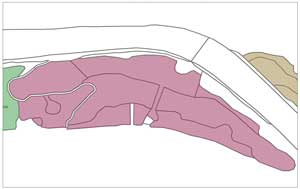
slough systems were likely to have had strong tidal forcing prior to alteration. Likely Former Tidal Wetlands Classified as Upland in the NWIIn the major diked tributaries of the Yaquina estuary—Boone Slough, Nute Slough, Depot Slough, and Olalla Slough—low-elevation land surfaces were extensive and were classified as upland in the NWI. These lands generally were less than 9 ft NAVD88. Similar low-elevation lands classified as upland in the NWI were identified in the middle and upper Alsea estuary. It seems likely that these were once tidal wetlands. However, the hydrology is currently altered by tide gates and extensive ditching and diking, so field investigation would be needed to determine whether these low-elevations lands are currently wetlands, and if so, their correct Cowardin et al. classification. We added these low-lying former tidal wetlands to the Enhanced NWI maps by cutting the upland polygon at an elevation of 11 ft NAVD88 based on the LiDAR data, using Editor/Split in ArcMap. An 11 ft elevation cutoff was used for consistency with the previously described LiDAR analysis (table 2). In lieu of a Cowardin et al. classification, the code FTW (Former tidal wetland) was assigned to these polygons, with the note "likely former tidal wetland/tidal waters of the State". The former tidal wetland polygons also were added to the Prioritization Sites by merging them with the adjacent NWI polygons, as described in section, "Creation of GIS Data for 1999 Tidal Wetland Prioritization Sites". Creation of GIS Data for 1999 Tidal Wetland Prioritization SitesAs described in section, "Project Goals and Objectives", one goal of this study was to generate GIS data (shapefiles) for the prioritization sites defined in the 1999 tidal wetland prioritization for the Yaquina and Alsea estuaries (Brophy, 1999) and characterize any major changes at the prioritization sites since 1999. The 1999 study identified and characterized current and likely former tidal wetlands in the Yaquina and Alsea estuaries, and divided the wetlands into 78 sites suitable for action planning purposes (43 in Yaquina, 35 in Alsea). These sites are referred to as prioritization sites in this report. The 1999 study then used ecological criteria to prioritize these 78 sites for conservation and restoration activities. Paper maps of the approximate locations of the 78 prioritization sites were provided with the 1999 report, but no GIS data were produced. The current project updated the 1999 study by providing GIS layers of the prioritization sites. The 1999 project and the current study are intended for use in strategic planning of voluntary conservation and restoration efforts; note however, that these products are not intended for regulatory use (Brophy, 1999). Consistent with the Oregon Estuary Assessment method (Brophy, 2007a), the 1999 study and the current study included emergent, scrub-shrub, and forested wetlands, but algal beds, seagrass beds, and mudflats were not included. GIS mapping and characterization of prioritization sites for the current study drew upon many data sources. Primary data sources were the LiDAR-derived elevations, NWI maps, and aerial photographs previously described. Other data included mapping of tidal wetlands and potential tidal wetlands provided by Scranton (2004), historical vegetation data, other GIS and tabular data sources, and expert local knowledge of the two estuaries derived from previous field studies ((Brophy, 2003, 2004, 2007b, 2007c, 2009; Brophy and Christy 2008, 2009; Brophy and others, 2011). The Oregon Watershed Assessment Manual, Estuary Assessment module (Brophy, 2007a) describes in detail how prioritization sites are created. Because individual NWI polygons are too small and numerous, they were merged to form larger analysis units based on hydrology, alterations, and land use history (fig. 3). These units (prioritization sites) are suitable for planning wetland restoration and conservation actions at the basin scale. In some cases, a prioritization site consisted of a single NWI polygon. However, in a few cases NWI polygons were split because of differences in the level of habitat alteration within a single polygon. Details on methods for defining prioritization sites are described in Brophy (2007a). The availability of LiDAR-derived elevations and recent aerial photography enabled identification of several new prioritization sites that had not been identified in the 1999 study (see section, "New Prioritization Sites Added to 1999 Study"). New prioritization sites were created only if the underlying NWI polygons totaled more than 1 acre.
Action planning for wetland restoration and conservation requires knowledge of conditions such as habitat alterations, dominant vegetation, land use, and potential restoration actions. The 1999 prioritization for the Yaquina and Alsea estuaries (Brophy, 1999) provided this information for each prioritization site in spreadsheet format. These prioritization site characteristics (table 2) were transferred as attributes to the GIS data generated in this project. In addition, major changes in prioritization site conditions since 1999 were identified through interpretation of the LiDAR data and aerial photographs, and by incorporating expert local knowledge, as previously described. These changes were listed as attributes in the prioritization site GIS shapefiles (attributes 8, 11, 13, 16, 18, 20, and 22 in table 4). Table 4. Table of attributes for GIS layer of prioritization sites to accompany 1999 tidal wetland prioritization. [Note: the value "n/a" for any attribute indicates that field was not used in the 1999 report.]
|
First posted May 10, 2013
For additional information contact: Part or all of this report is presented in Portable Document Format (PDF); the latest version of Adobe Reader or similar software is required to view it. Download the latest version of Adobe Reader, free of charge. |
||||||||||||||||||||||||||||||||||||||||||||||||||||||||||||||||||||||||||||||||||||||||||||||||||||||||||||||||||||||||||||||||||||||||||||||||||

![]() U.S. Department of the Interior |
U.S. Geological Survey
U.S. Department of the Interior |
U.S. Geological Survey
URL: http://pubsdata.usgs.gov/pubs/of/2012/1038/methods.html
Page Contact Information: GS Pubs Web Contact
Page Last Modified: Friday, 10-May-2013 12:37:32 EDT