

A generalized framework for inferring river bathymetry from image-derived velocity fields
Links
- More information: Publisher Index Page (via DOI)
- Document: XML
- Open Access Version: USGS Accepted Manuscript
- Download citation as: RIS | Dublin Core
Graphical Abstract

A map of water depth in the Tanana River near Nenana, Alaska, produced using the Depths Inferred from Velocities Estimated by Remote Sensing (DIVERS) framework.
1. Introduction
Information on flow conditions in river channels plays a key role in applications ranging from water management and flood hazard assessment to habitat mapping. Measuring depth, velocity, and discharge directly in the field can be laborious, often prohibitively expensive, and sometimes dangerous. These limitations are particularly acute in locations that are difficult to access, which can make site visits to gaging stations logistically challenging. Remote sensing techniques provide an alternative in these settings, with potentially meaningful advantages in terms of spatial coverage, efficiency, and safety. Exploring various non-contact approaches to measuring streamflow has thus emerged as a primary research objective for hydrologic monitoring agencies (Conaway et al., 2019). Motivated by this operational need, we developed a flexible workflow for inferring multiple river characteristics from remotely sensed data.
This approach exploits advances in our ability to map one attribute, velocity, to produce spatially distributed estimates of another attribute that is more difficult to measure via remote sensing: depth. Techniques such as particle image velocimetry (PIV) were first applied to natural channels nearly 20 years ago (e.g., Muste et al., 2008) and are now widely used (e.g., Strelnikova et al., 2023). Estimating velocities from image time series relies upon distinct water surface features that can be tracked from frame to frame, but clear-flowing streams often lack natural tracers and seeding with artificial particles can be impractical (e.g., Biggs et al., 2022). Successful image velocimetry also requires careful selection of acquisition and processing parameters (Bodart et al., 2024; Legleiter and Kinzel, 2024a). Granting these caveats, image-based techniques have been shown to be effective in a range of river environments using data from helicopters (e.g., Legleiter and Kinzel, 2020), uncrewed aircraft systems (UAS) (e.g., Eltner et al., 2021), and even satellites (e.g., Masafu et al., 2023). In addition, various image velocimetry algorithms have been incorporated into readily available software (e.g., Patalano et al., 2017; Legleiter and Kinzel, 2023; Ljubičić et al., 2024). With the development of such tools, remote sensing of flow velocities has become a mature technology that could support indirect estimation of river bathymetry.
The ability to infer water depth from some external source of information could be valuable because mapping bathymetry from remotely sensed data remains problematic in large, turbid rivers. Both spectrally-based depth retrieval methods and bathymetric lidar are restricted to relatively clear, shallow channels (e.g., Legleiter and Harrison, 2019). Ground-penetrating radar could be used to measure depth in more turbid settings, but the conductivity of the water can be a limiting factor and this approach provides coarse spatial resolution with reduced coverage near banks and can be impractical to apply (Spicer et al., 1997; Costa et al., 2006; Fediuk et al., 2022; Bandini et al., 2023). Because clear-flowing streams conducive to passive optical remote sensing are not well-suited to image velocimetry, and vice versa for turbid rivers, mapping both bathymetry and velocity simultaneously with a single sensor continues to be an elusive goal, although some progress has been made in estimating depth from surface velocity and turbulence (e.g., Johnson and Cowen, 2016) or surface wave characteristics (e.g., Dolcetti et al., 2022). Legleiter and Kinzel (2021a), abbreviated as LK21, proposed a solution to this either/or conundrum that involved estimating depth from image-derived velocity fields. We referred to this framework as DIVERS, short for Depths Inferred from Velocities Estimated by Remote Sensing. In this study, we build upon and generalize the DIVERS workflow.
The DIVERS approach is based on a flow resistance equation that relates depth to velocity and can thus yield detailed depth maps with a spatial resolution equivalent to that of the velocity field used as input. In addition, a new approach can also provide greater spatial coverage: mapping velocities from a fixed-wing aircraft traveling along a river rather than a helicopter or UAS hovering above the channel. This moving aircraft river velocimetry (MARV) framework is described in Legleiter et al. (2023, abbreviated LE23) and, in combination with DIVERS, creates new possibilities for remote sensing of both velocities and depths. The principal aim of this study is to integrate the two workflows and assess their potential for large-scale mapping of multiple river characteristics.
Our objectives herein are to refine the DIVERS framework and apply the workflow to a large river in Alaska as an additional proof-of-concept. More specifically, the following sections describe several improvements to DIVERS:
-
1. MARV provides continuous, spatially extensive, high resolution velocity fields that are a more appropriate input to DIVERS than patchwork velocity maps derived from a series of hovers distributed along a reach.
-
2. Transforming the image-derived velocity field to a channel-centered coordinate system allows hydraulic calculations to be performed on a regular grid using only the downstream component of each vector.
-
3. The optimization phase of the workflow, which previously focused on calibrating a single flow resistance coefficient, now allows for multiple free parameters and can be applied on a per-cross section (XS) basis.
-
4. Similarly, in addition to optimization to match a known discharge, we provide a new objective function to minimize the coefficient of variation of estimated discharges within a reach when the discharge is unknown.
We illustrate these new components via a case study and use field measurements to assess the accuracy of velocities estimated via MARV and depths inferred via DIVERS. In addition, we perform a sensitivity analysis to evaluate the robustness of the optimization algorithm to misspecification of initial parameter estimates and errors in the input variables. In the discussion, we revisit the assumptions underlying the DIVERS framework and consider the potential of the approach for remote sensing of velocity and depth in rivers.
2. Methods
2.1. Study area, field measurements, and remotely sensed data
This study builds upon previous work on central Alaska’s Tanana River, focused on a reach near the village of Nenana (Legleiter and Kinzel, 2020, 2021b,a; Legleiter et al., 2023). This river is conducive to image velocimetry due to an abundance of suspended sediment. This fine-grained material imparts a bright tone to the Tanana in the satellite image shown in Figure 1, whereas the relatively clear-flowing tributary entering from the south is much darker. On the Tanana, turbulence originating at the bed redistributes sediment within the water column to produce boils, vortices, and other water surface features expressed as patterns of color and texture. Tracking the motion of these features from frame to frame allows surface flow velocities to be estimated from an image sequence. The sediment boil vortices that serve as natural tracers obviate the need to seed the flow with artificial particles, which would simply not be practical on a large river (e.g., Detert et al., 2019).
Field measurements of flow depth and velocity were obtained on 18 August 2021, when the discharge recorded at the USGS gaging station (site no. 15515500) on the Tanana River at Nenana was 1,393 m3/s (U.S. Geological Survey, 2024). The field data were collected along eight cross sections (XSs) using a TRDI RiverRay (Teledyne Marine, Poway, CA) acoustic Doppler current profiler (ADCP), with two passes back and forth across the channel at each XS; each pass required 5-10 minutes to complete. This approach was convenient and relatively fast but also implied that the measurement time at any one location was substantially less than 30 seconds. Performing a section-by-section measurement with a longer occupation time at each position across the channel would have led to more reliable characterization of the vertical velocity profile but with the cost of increased overall measurement time. Given our emphasis on reach-scale spatial coverage and the limited resources available for this study, we prioritized efficiency in data collection but acknowledge that the relatively short averaging times were an important source of uncertainty for our field measurements of flow velocity. We used the Velocity Mapping Toolbox (VMT, Parsons et al., 2013) for post-processing, which involved fitting a mean XS to the boat track, smoothing the data both horizontally and vertically (using bin sizes of 1 m and 0.4 m, respectively), and calculating depth-averaged velocity vectors (Figure 2a). We used depths recorded by the ADCP (Figure 2b) to assess the accuracy of depths estimated via the DIVERS workflow.
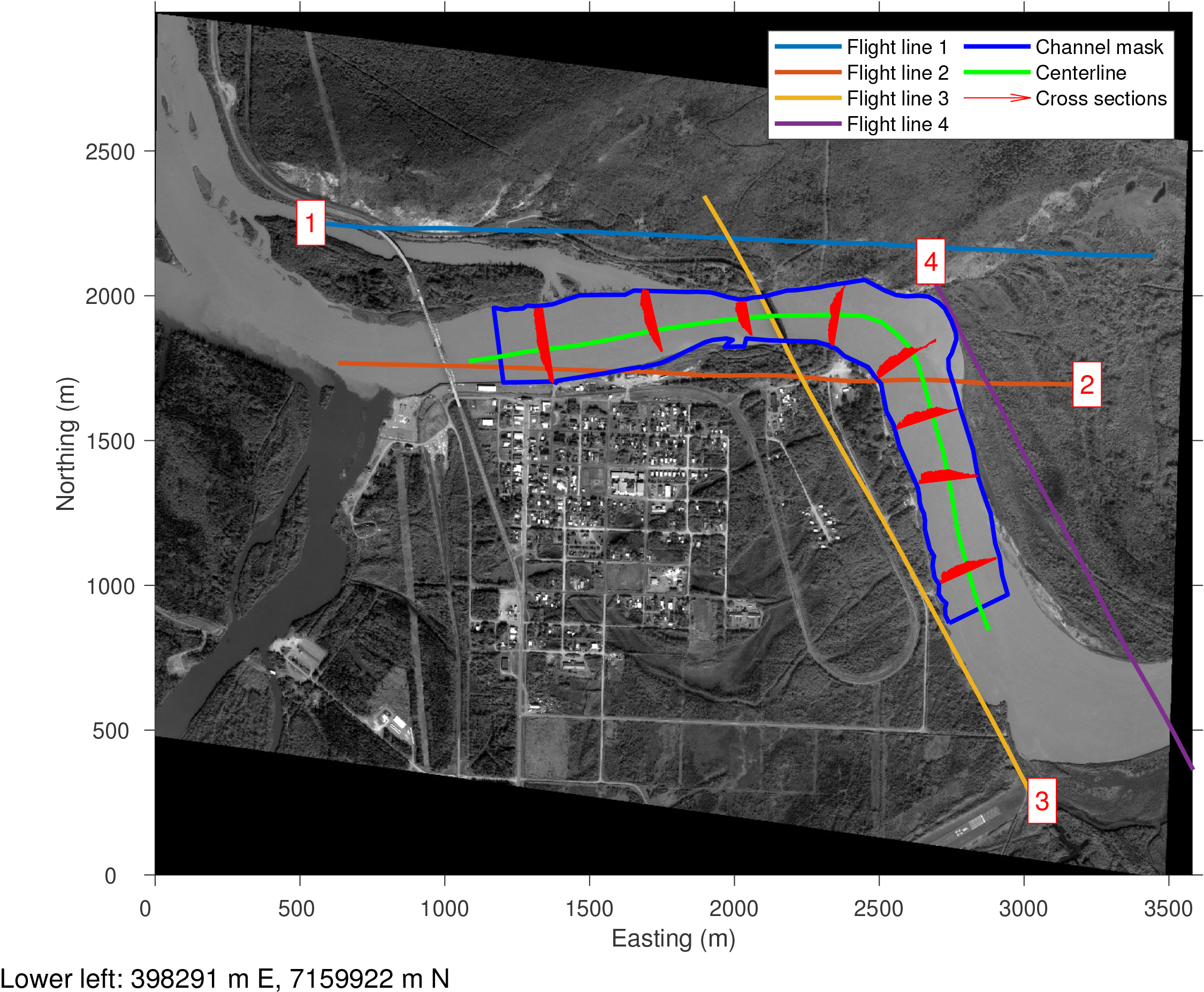
Study area on the Tanana River near Nenana, Alaska, with the four flight lines along which the images used for moving aircraft river velocimetry (MARV) were acquired. Also shown are the locations of field measurements of flow depth and velocity made with an acoustic Doppler current profiler (ADCP).
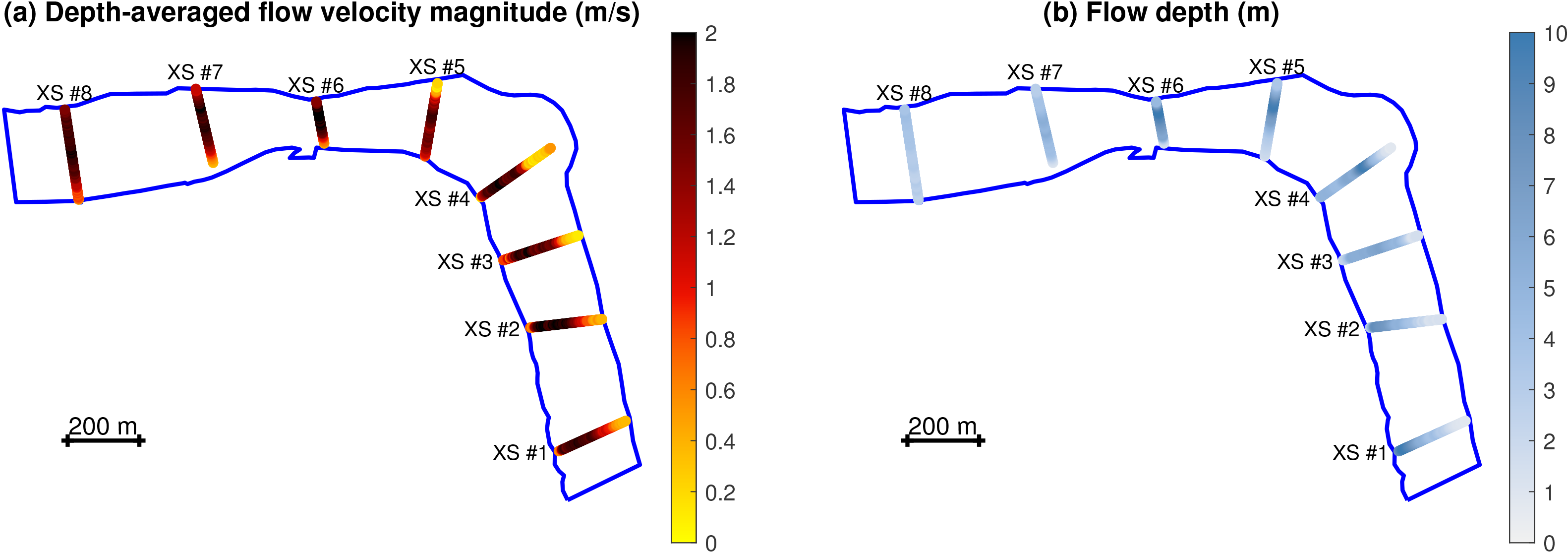
Field measurements of (a) velocity and (b) depth made along eight cross sections (XSs) of the Tanana River.
Images of the Tanana River were acquired from an aircraft on 19 August 2021, as described in greater detail in LE23. For this study, we used images captured by a Nikon 850 (Melville, NY) digital camera deployed from a flying height of 1,204 m above ground level along the four flight lines shown in Figure 1. The capture interval was set to 1.4 s, leading to approximately 90% overlap between frames along each flight line. The mission resulted in a total of 183 images with a ground sampling distance of 0.1 m that were orthorectified to serve as input for the MARV workflow. All the field measurements and images used in this study are available from Legleiter et al. (2022).
2.2. Moving aircraft river velocimetry (MARV)
Relative to the original MARV workflow described by LE23, the processing chain used in this study was streamlined in several ways for incorporation into the Toolbox for River Velocimetry using Images from Aircraft (TRiVIA) (Legleiter, 2024). For a more general discussion of MARV and its implementation in TRiVIA, please refer to LE23 and Legleiter and Kinzel (2024b). Herein, we briefly highlight some key refinements.
The first two steps in MARV are to establish the spatial footprint of each frame and then compare the resulting footprint polygons to identify overlapping frames. This analysis was performed using a “rolling” technique that involves extracting only those frames within a window of specified length (i.e., number of frames) and identifying the area of overlap common to all images within the current window. The rolling window then moves forward by a number of frames also set by the user, referred to as the jump. For each window, the individual images are cropped to the area of overlap, masked using a manually digitized channel polygon, and enhanced using a contrast stretch and smoothing filter to facilitate detection and tracking of water surface features.
The end result of these pre-processing steps is, for each frame range, a masked, water-only image sequence that captures the same area of the river at several instances in time and is thus suitable for velocity estimation. We used an ensemble correlation particle image velocimetry (PIV) algorithm adapted from PIVlab (Thielicke and Stamhuis, 2014). This approach offers significant advantages in terms of computational efficiency and performance when the density of trackable water surface features is low (Thielicke and Sonntag, 2021). The initial velocity field for each frame range was filtered to remove spurious vectors using the settings listed in Table 1 and then infilled and smoothed using algorithms from PIVlab (Legleiter and Kinzel, 2023).
Table 1.
Image characteristics and moving aircraft river velocimetry parameters.Within the MARV framework, a PIV analysis is performed and a separate image-derived velocity field produced for each individual frame range. Because many of these frame ranges overlap one another, the next stage of the workflow involves combining the initial PIV output from all frame ranges. This process leads to an aggregated velocity field that is dense but also scattered, irregular, and unwieldy for practical applications. To provide a more concise summary, we created a grid of prediction locations with a spacing, denoted by ∆, of 10 m, the same as the output vector spacing used for PIV. All the original vectors within 0.5∆ of a given node of the prediction grid in both the east and north directions were associated with that node and used to compute ensemble median vectors and median absolute deviations. This aggregation process involved pooling velocity vectors derived from images acquired along different flight lines and thus provided denser coverage in areas of sidelap between passes of the aircraft.
2.3. Transformation from Cartesian to channel-centered coordinates
For this study, we added a new component to the DIVERS framework: transformation of the image-derived velocity field to a channel-centered coordinate system defined by streamwise s and normal n axes (Smith and McLean, 1984; Legleiter and Kyriakidis, 2006). This process places the velocity field within a local, relative frame of reference by assigning each velocity vector to a specific distance along and across the channel, with the s coordinate originating at the upstream end of a channel centerline digitized by the user and the n coordinate increasing from the centerline toward the left bank from the perspective of an observer facing downstream; n < 0 for points to the right of the centerline.
In the context of DIVERS, transforming the velocity field to s, n coordinates serves two purposes. First, whereas the original east and north components of each vector could have any orientation relative to the actual flow direction, transformation allows vectors to be resolved into more physically meaningful streamwise and normal components. We obtained these components by modifying the Legleiter and Kyriakidis (2006) coordinate transformation algorithm to also output the unit tangent and unit normal vectors for each centerline vertex. As shown in Figure 3, the tangent vector represents the direction θ of the channel centerline and the normal vector points in the direction ϕ of the left bank. The streamwise us and normal un components of each velocity vector u are then calculated as
where U is the magnitude of the velocity vector and ω refers to its orientation in the original Cartesian coordinate system. Calculating us isolates the vector component that contributes to the discharge, whereas using the magnitude U would implicitly assume that all flow is directly downstream.
The second reason for transforming from x, y to s, n coordinates is to facilitate subsequent analyses by projecting the velocity field onto a convenient channel-centered grid. Because the MARV prediction grid was no longer regular after transformation to channel-centered coordinates, we created a new rectilinear grid in the s, n space with a regular spacing of 0.5∆ and nodes spanning the full length of the reach in the s direction and the entire width of the channel in the n direction. We then interpolated the transformed velocity field, defined at the s, n points resulting from coordinate transformation of the original MARV prediction grid, onto the nodes of this new grid by defining one interpolant for us and another for un. This approach results in a grid where each column has a constant value of s and thus represents a channel XS, which is the basic unit of analysis for the hydraulic calculations that comprise the next stage of the workflow. Although in general transformation from Cartesian to channel-centered coordinates could result in overlapping cross sections in tight bends with a small radius of curvature relative to the channel width, the algorithm described by Legleiter and Kyriakidis (2006) can be parameterized to avoid this issue. For this study, we confirmed that the 5 m spacing between centerline nodes we used resulted in cross sections that did not overlap.
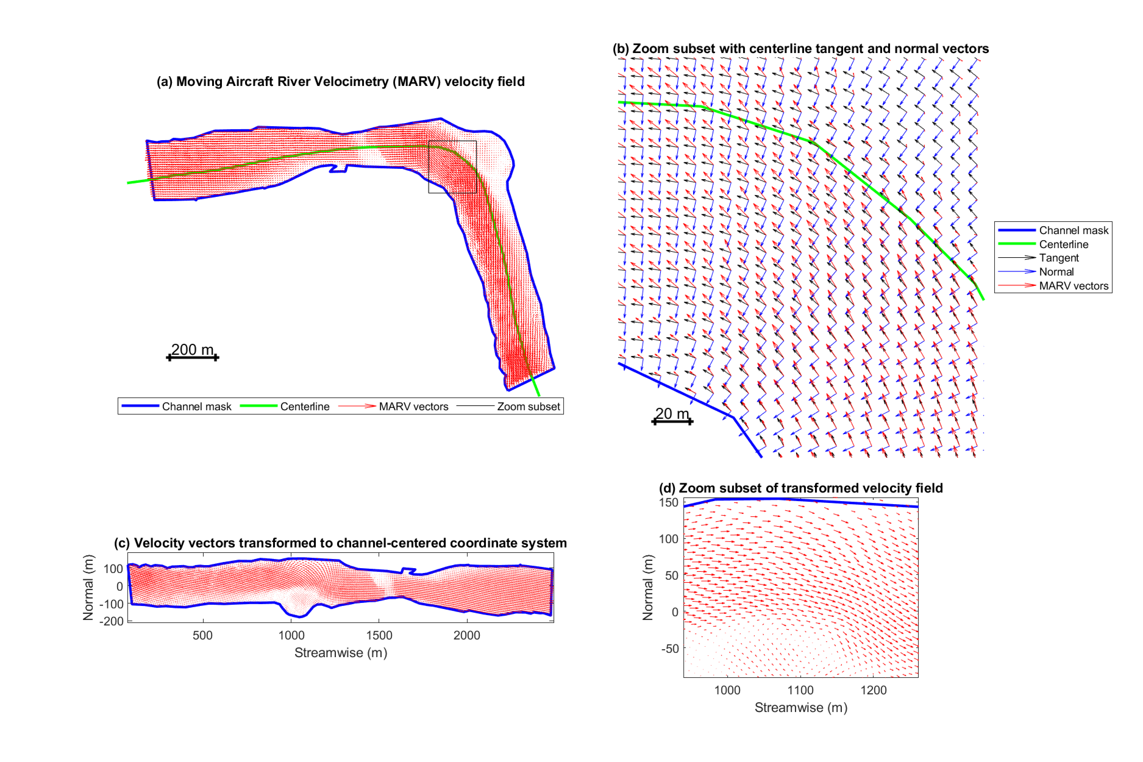
Transformation of the velocity field from Cartesian spatial coordinates to a channel-centered reference frame. (a) Velocity field inferred via moving aircraft river velocimetry (MARV) in the original spatial coordinate system. (b) Zoom subset showing the centerline tangent and normal vectors used to project velocity vectors into streamwise and normal components. (c) Velocity field transformed to the channel-centered reference frame with along- (streamwise) and across-stream (normal) coordinates. (d) Zoom subset of the transformed velocity field.
2.4. Calculating depth from velocity via a flow resistance equation
The core of the DIVERS framework is an expression that relates the surface velocity at a given location within the channel to the depth at that location. We begin with a power law velocity profile given by
where u(z) is the flow velocity at a height z above the channel bed, u∗ is the shear velocity, k is a roughness length scale, and a and m denote an assumed or fitted coefficient and exponent, respectively. LK21 showed how this expression can be used to calculate both the velocity us at the water surface and the depth-averaged velocity U . Moreover, the ratio of U to us, which is the definition of the velocity index α (e.g., Biggs et al., 2023), is related to the exponent m, which can thus be used to convert image-derived surface velocities to depth-averaged velocities for estimating discharge:
The following expression is then used to infer the flow depth H from the velocity at the water surface and the slope of that surface, denoted by S:
This relation was derived by rearranging the equation for surface velocity (2 in LK21) and making a substitution for the shear velocity: , where g is acceleration due to gravity. In this study, we used the streamwise component of the velocity vector rather than its magnitude to include only the downstream-directed portion of the flow when calculating discharge. The subscript s in us thus represents both the vertical position at the water surface and the streamwise component of the velocity vector. Under the assumption that the power law velocity profile given by Equation (2) adequately describes the flow at any location within the channel, Equations (3) and (4) provide a means of calculating the depth-averaged velocity and flow depth, respectively, from an image-derived velocity field and the water surface slope. A continuous map of depth throughout the reach can be produced by applying these expressions to each node of the us grid.For the optimization phase of the DIVERS workflow, the product of depth and velocity is integrated laterally across the channel to compute discharge. Assuming a uniform width increment ∆w between adjacent “verticals,” the discharge Q at each XS can thus be calculated as
where j indexes the N columns of the s, n grid. Similarly, i indexes the M rows of the s, n grid, which correspond to the individual verticals along the jth XS. The width increment ∆w is equivalent to the spacing between grid nodes in the n direction. Substituting Equations 3 and 4 into Equation 5 yields the following expression for discharge at XS j:2.5. Optimization and depth retrieval
The preceding development provides a foundation for remote sensing of water depth, by way of surface velocity, and potentially estimating river discharge. To do so, the variables us and S must be measured and the parameters a, m, and k must be estimated. For us, we used median velocity vectors from MARV. As in LK21, we used a slope of 0.00014, measured from a 2019 lidar DEM of the Tanana River. To infer values of a, m, and k, we used an optimization approach that required an initial estimate of each parameter. For a, we used a plausible initial value of 6.43 derived by Ferguson (2007) based on a large compilation of field data. For m, which is related to the velocity index α = 1/(m + 1), the most widely used α value of 0.85 (e.g., Biggs et al., 2023) corresponds to a default of 0.1765 for m. Alternatively, if measured velocity profiles are available, m can be calculated using the QRev software package (Mueller, 2016). For this study, we used ADCP data from the Tanana River to obtain a site-specific α value of 0.8883 (LE23 Table S1), which corresponds to m = 0.1257. Finally, to obtain an initial estimate of the roughness length scale we back-calculated k from bulk hydraulic quantities recorded during site visits to gaging stations, as described by LK21. For the USGS gage on the Tanana River at Nenana, the site visit closest to when the images used in this study were acquired was made on 13 July 2021 and led to a calculated k value of 0.00176 m.
The generalized DIVERS framework outlined herein provides numerous options for parameter estimation and is much more flexible than the initial version from LK21. For example, the optimization can be based on either of two objective functions, depending on whether a known discharge is available. Similarly, optimization can be performed globally to obtain reach-averaged parameter values or locally to obtain an estimate of a, m, and k for each individual XS. One can also select which parameters are free to vary during the optimization and which are held constant. Many variants are thus possible, but in this study we focused on two specific versions of DIVERS distinguished from one another by the objective function driving the optimization and whether m was variable or fixed; a and k were always variable.
The first objective function is designed to match a known discharge by iteratively adjusting a, m, and k to minimize the root mean squared error (RMSE) between the known discharge Q and the discharges Q̂j calculated from the image-derived velocity field for each of the N XSs via Equation 6. This objective function, which we refer to as match Q, is given by
where P is a 3 × N parameter matrix with a separate column for each XS to allow for local optimization. We used the same initial parameter estimates for all XSs, such that aj = a for all j and likewise for m and k.We also considered a second objective function that does not require a known discharge. In this case, the optimization process can instead be guided by a continuity constraint: discharge should be constant throughout a reach in which tributary inputs and hyporheic exchange are negligible. A plausible objective is to minimize the variance of the calculated discharges over the N XSs. However, the variance cannot be used directly because the variance of smaller numbers is always less than that of larger numbers. We addressed this issue by using the coefficient of variation of discharge, denoted by CV(Q), to scale variations in Q by their mean and thus prevent the optimization algorithm from gravitating toward very small discharges. The objective function for this alternative approach, which we refer to as minimize CV(Q), is given by
where σ(Q̂) and µ(Q̂) are the standard deviation and mean, respectively, of the estimated discharges Q̂j for the N XSs. P is as defined above, but in this case we held m fixed during the optimization.The Nelder-Mead simplex algorithm, as implemented in the MATLAB fminsearch routine (Lagarias et al., 1998; The MathWorks, Inc., 2024), was used to minimize
the selected objective function. We modified the default settings to use more stringent
convergence criteria and allow for more iterations. We used a tolerance of 0.0001
for both the parameter matrix P adjusted during the optimization and the objective function given by Equation 7 or
8. The maximum number of function evaluations and the maximum number of iterations
were both set to 10,000. The algorithm terminated when the tolerance on P or the selected objective function was satisfied or when the maximum number of function
evaluations or iterations was reached.
Once the optimization process was complete, we used the resulting parameter values to calculate H at each node of the s, n grid from us at that location using Equation 4. To transform the resulting depth estimates back into Cartesian coordinates, we created an interpolant for H on the channel-centered grid and evaluated this interpolant at the s, n coordinates obtained by transforming the nodes of the original x, y velocity grid to the channel-centered frame of reference. This approach provided a depth estimate at each node of the original MARV prediction grid.
2.6. Accuracy assessment of image-derived velocities and depths
To evaluate the reliability of image-derived velocity estimates, we compared the median surface velocity vectors from MARV to in situ observations of depth-averaged velocity made with an ADCP. For each node of the MARV prediction grid, we identified all field measurements located within 0.5∆ of that node and averaged them. For consistency with previous work on the Tanana River (Legleiter and Kinzel, 2020, 2021b; Legleiter et al., 2023) and to avoid imposing an assumed value of α, we did not apply a velocity index to convert from surface to depth-averaged velocities. We used the resulting paired velocity magnitudes to perform an observed (ADCP) versus predicted (MARV) regression that served to quantify the level of agreement between velocities recorded in the field and inferred from images. To obtain additional further information on precision and absolute accuracy, we calculated the RMSE and mean bias. The bias was defined by subtracting the velocity measured by the ADCP from that estimated via MARV. We expressed these metrics in non-dimensional form by dividing them by the mean of the ADCP measurements, leading to normalized RMSE and mean bias values that represent fractions of the reach-averaged velocity.
To assess the accuracy of depth estimates inferred via DIVERS, we used field measurements of water depth made with the ADCP. For each of the eight XS surveyed in the field, we calculated the RMSE and mean bias between the observed (ADCP) and predicted (DIVERS) depths and obtained normalized RMSE and bias values by dividing by the mean of the measured depths along each XS. In addition, we calculated both metrics using the entire reach-aggregated data set by pooling observations from all eight XSs. To compare the two DIVERS variants, we also performed a regression of the mean of the depths measured in the field for each XS versus the mean of the depths estimated by DIVERS for each XS. These regressions had a small sample size (n = 8 XS) but quantified the overall level of agreement between the depths predicted via DIVERS and those observed with the ADCP.
2.7. Sensitivity analysis
The optimization algorithm searches a multidimensional parameter space to find the specific values of a, m, and k that minimize the selected objective function. To better understand how this process identified solutions, we conducted a series of sensitivity analyses. An additional goal was to assess whether the DIVERS framework was robust to misspecification of the initial parameter estimates. We also evaluated how errors in the two measured quantities, us and S, would affect depth estimates. More specifically, we used a differential approach to gain insight as to how depths calculated via Equation 4 were affected by changes in the three parameters and two input variables. In general, a first-order approximation of the change in the value of f (x) associated with an incremental change ∆x in x is given by:
where f ′(x) is the derivative of f (x) with respect to x. In this case, f (x) is given by Equation 4 and x represents a, m, k, us, or S. We differentiated Equation 4 with respect to each of these quantities to obtain the following partial derivatives, which correspond to f ′(x) in Equation 9:To illustrate how changes in each parameter or variable affect depths calculated via Equation 4, we varied each of the five quantities from one half to twice the base case value listed in Table 2 while holding the other four parameters/variables constant. In practice, the range of possible values for each parameter could be less than the 50% - 200% range we used. The following analysis is thus conservative in the sense that such a broad range of values is likely to encompass the plausible range of values for a specific application. Because information on appropriate ranges would seldom, if ever, be available a priori, we used a consistent 50% - 200% range to provide some general insight. For us, we multiplied the surface velocities at all grid nodes by the same factor such that the magnitude increased or decreased but the spatial pattern of the velocity field remained unchanged. This approach captured the effects of a spatially uniform, consistent bias relative to the base case velocity field but not the impacts of any more complex, spatially varying random or systematic errors. We also used Equations 10–14 to calculate the incremental change in depth ∆H corresponding to an incremental change in a, m, k, us, or S for the same range of values. Finally, because the three parameters and two input variables have different units and absolute magnitudes, we recast the analysis in non-dimensional terms to more clearly highlight which quantities have a greater impact on predicted depths. We scaled each parameter/variable by its base case value and divided the calculated depths and changes in depth by the base case depth H0.
Table 2.
Base case values of parameters and variables used in sensitivity analysis. MARV= moving aircraft river velocimetry.To assess the sensitivity of DIVERS output to the initial parameter estimates, surface velocity field, and slope provided as input, we performed a series of DIVERS runs with different values of these inputs. Relative to the base case values listed in Table 2, we performed runs using inputs multiplied by factors of 0.5, 0.75, 0.9, 0.95, 1, 1.05, 1.1, 1.25, 1.5, representing departures of up to 50%. To quantify the impact of these altered inputs on depths estimated via DIVERS, we calculated the normalized RMSE and mean bias between the depths measured in the field and those inferred from the velocity field on a per-XS basis for each of the eight transects and for the reach-aggregated data set. Finally, for the scenario where the discharge is not known a priori and the goal is to minimize the variability of estimated discharges, we also examined the effects of varying the initial values of a, k, us, and S on the mean of the resulting per-XS discharge estimates.
3. Results
3.1. Reach-scale velocity mapping
The MARV workflow led to a coherent, detailed velocity field for the 2.5 km reach of the Tanana River shown in Figure 4a. The subset highlighted in Figure 4b illustrates the ability of ensemble PIV to capture subtle features like the eddy that occurred where the channel curved to the west and flow recirculated along the outer bank. In addition, aggregating the velocity vectors from the various frame ranges provided a metric of variability: the median absolute deviation of the estimates contributing to each node of the MARV prediction grid. Median absolute deviations tended to be greater where the flow field was more complex (Figure 4c), such as along the margin of the eddy (Figure 4d). The ability to not only efficiently map long reaches but also resolve local details is a key advantage of the MARV approach relative to hover-based image velocimetry or conventional field methods.
Accuracy assessment of MARV output indicated strong agreement between the depth-averaged velocity magnitudes oberved in the field with an ADCP and those inferred from images via MARV, with an R2 of 0.81 (Figure 5). The normalized RMSE and mean bias of the image-derived velocity estimates were 0.174 and -0.022, respectively, implying that the median velocity vectors from MARV were reasonably precise, within 17.4% of the reach-averaged mean velocity, and biased by only 2.2%. The negative sign of the mean bias indicates that MARV tended to slightly underpredict the depth-averaged velocities measured in the field.
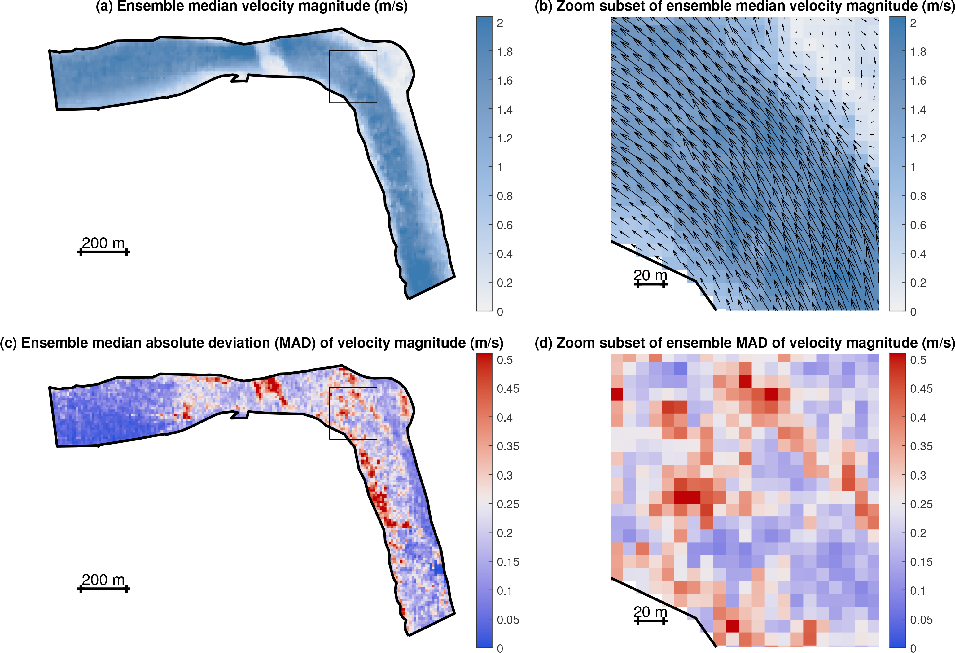
Moving aircraft river velocimetry (MARV) output for the Tanana River, including both ensemble median velocity vectors (a and b) and ensemble median absolute deviations (c and d).
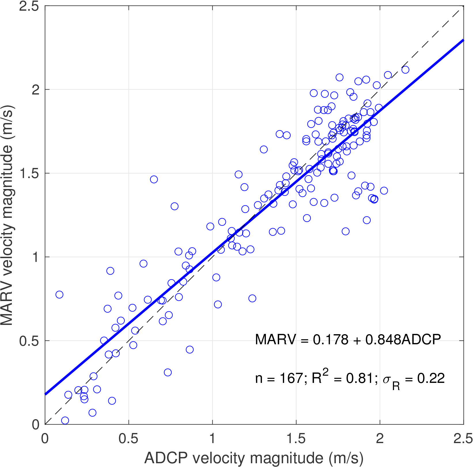
Accuracy assessment of moving aircraft river velocimetry (MARV)-derived velocity magnitudes via comparison to field measurements made with an acoustic Doppler current profiler (ADCP).
To make use of MARV output within the DIVERS framework, we transformed the image-derived velocity field to a channel-centered coordinate system more conducive to hydraulic calculations. We also resolved each velocity vector into downstream and cross-stream components as described in Section 2.3. Several additional steps were required to prepare the velocity field for depth estimation. We first cropped the s, n grid to encompass only that portion of the study area for which field measurements were available. Another section was replaced with no data values to exclude a bridge that obscured the water surface and thus precluded image velocimetry. We also trimmed the upper and lower ends of the reach to omit partial transects where the transformed MARV prediction grid did not extend all the way across the channel. This step ensured that each column of the grid represented a complete XS suitable for discharge calculation. The final surface velocity field used to infer depths is shown in Figure 6.
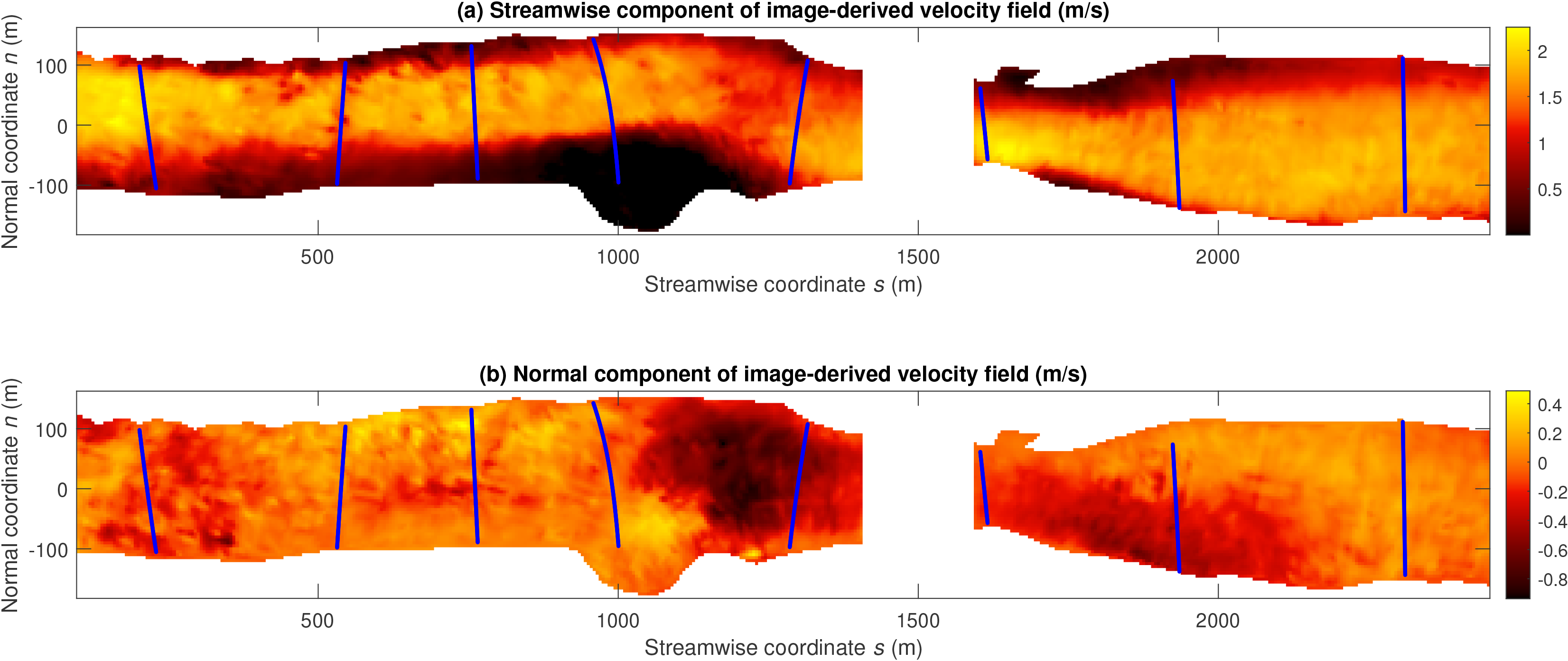
Image-derived velocity field following transformation to the channel-centered s, n coordinate system, resolved into along- (a) and (b) across-stream components, referred to as streamwise s and normal n, respectively. The locations of field measurements of flow depth and velocity made along eight cross sections (XSs) are indicated with blue dots.
3.2. Inferring depths with different versions of DIVERS
We used the image-derived velocity field along with the initial parameter estimates and water surface slope listed in Table 2 to estimate depths using both DIVERS variants. Figure 7 shows the resulting bathymetric maps in channel-centered coordinates. The void from s = 1415 -1915 m is where the bridge blocked the river from view. Another gap in coverage occurred farther upstream, from s = 880 - 1210 m and for n coordinates less than about -25 m, where a large eddy formed near the bend apex and flow recirculated back upstream along the outer bank. The streamwise component of the velocity vectors in this area were thus negative, which led to imaginary numbers in Equation 4 and forced us to exclude this portion of the reach. Aside from these two exceptions, the DIVERS workflow led to plausible, spatially coherent depth estimates that were generally shallower along the margins of the channel and deeper in the thalweg; the greatest predicted depths occurred immediately downstream of the bridge.
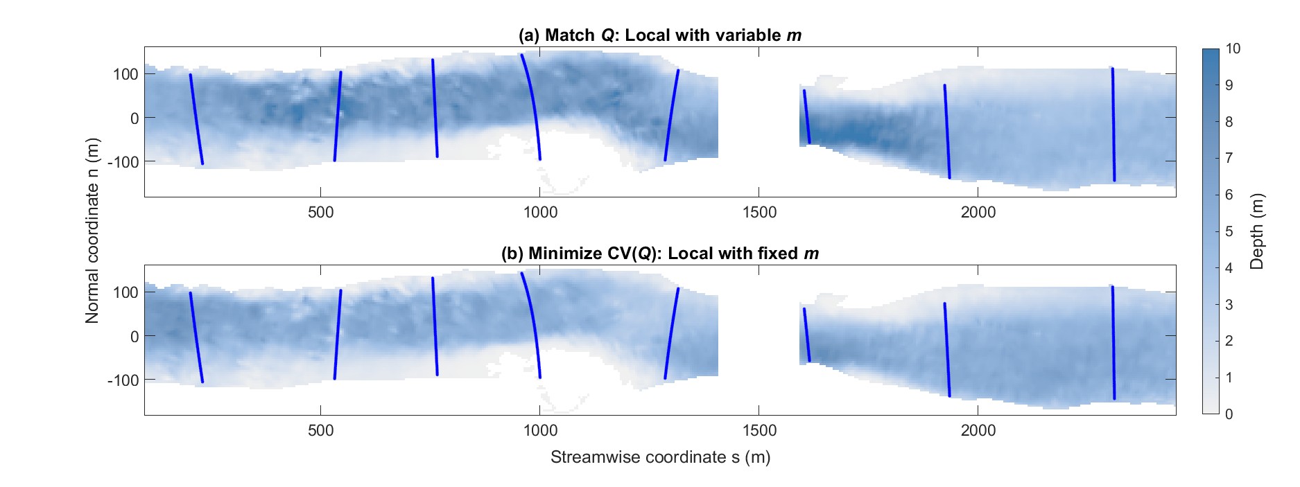
Channel-centered bathymetric maps for two different implementations of the Depths Inferred from Velocities Estimated via Remote Sensing (DIVERS) framework: (a) matching a known discharge Q with variable m; and (b) minimizing the coefficient of variation of estimated discharges, abbreviated CV(Q), with fixed m.
We also plotted cross-sectional profiles to compare depth estimates from the two DIVERS variants to one another and to the depths measured in the field (Figure 8). Several consistent patterns were observed across the eight XSs surveyed with the ADCP. For example, the channel shape and cross-stream position of the maximum image-derived depth generally coincided with those recorded in the field, implying that in this study area one of the key assumptions of DIVERS — local proportionality between water surface velocity and depth — was appropriate for the most part. However, an exception occurred where this simple assumption failed to account for more complex hydrodynamic processes near the bend apex (XS #4).
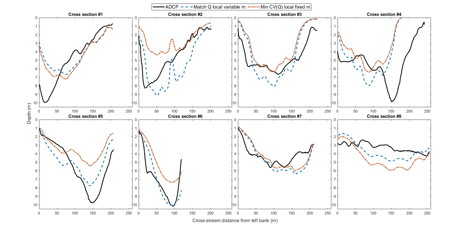
Comparison of cross sections (XSs) surveyed in the field with an acoustic Doppler current profiler (ADCP) and estimated via the Depths Inferred from Velocities Estimated via Remote Sensing (DIVERS) framework designed to match a known discharge Q or minimize the coefficient of variation of estimated discharges, denoted min CV(Q), with the power law velocity profile exponent m either variable or fixed.
Both versions of DIVERS produced similar depth estimates that agreed reasonably well with ADCP measurements. Qualitatively, the discharge-matching objective function appeared to lead to the most accurate depth estimates, particularly for the XSs (5-8) downstream of the bend apex where secondary flows were less pronounced and the uniform flow approximation was more realistic. Regardless of the particular variant of DIVERS employed, the resulting depth estimates had the same cross-sectional shape. Although the two implementations led to depth estimates with different magnitudes, the spatial pattern of the bathymetry did not vary because the same image-derived velocity field was used as input. The spatial structure of this velocity field was mirrored in both versions of the bathymetry because the depth at a given location was assumed to be proportional to the velocity at that location.
To quantify this comparison, we calculated the normalized RMSE and mean bias relative to the field measurements for each individual XS and for the reach as a whole by aggregating data from all eight XSs. The results of this analysis are summarized in Figure 9, where each DIVERS variant is represented by a distinct bar color for each XS (the first eight groups of bars) and the reach-aggregated data set (the last group of bars). As was evident in the cross-sectional profiles, allowing a, m, and k to vary on a per-XS basis to reproduce the known discharge led to the smallest normalized RMSE for the reach-aggregated data set (0.400) and a mean bias near zero. Although depth estimates were more precise for some of the XSs, with a minimum of 0.188 for XS #6, the reach-aggregated normalized RMSE of 40% implied that DIVERS did not yield highly reliable depth estimates at the level of an individual grid node (i.e., with a spatial resolution on the order of 5-10 m).
To assess whether DIVERS could provide useful bathymetric information at a cross-sectional level, we calculated the mean of the depths estimated via the two DIVERS variants along each XS and compared these XS mean depths to those computed from the field data. We then performed regressions of observed (ADCP) versus predicted (DIVERS) XS mean depths for both versions of DIVERS. The results of this analysis are summarized graphically in Figure 10, where the individual data points and corresponding best-fit lines are distinguished by marker style and color and the R2 values for each regression are listed in the legend. The only variant that led to a statistically significant (p < 0.05) correlation between image-derived depth estimates and field measurements, with an R2 of 0.748, was the discharge-matching approach that allowed m to vary. This result suggests that if a known discharge is available, the DIVERS workflow can provide accurate cross-sectional mean depths without having to assume or calibrate a parameter (m) describing the shape of the velocity profile. The regression line for the fMQ variant has a shallower slope and greater intercept than the one-to-one line of perfect agreement included as a reference in Figure 10, indicating that depths tended to be overpredicted at shallower XSs and underpredicted at deeper XSs. Optimization based on fCVQ did not lead to a strong relationship between observed and predicted XS mean depths. However, the mean of the estimated discharges calculated for each XS along the reach was 1,258 m3/s, within 10% of the known Q even though it was not used as a constraint.
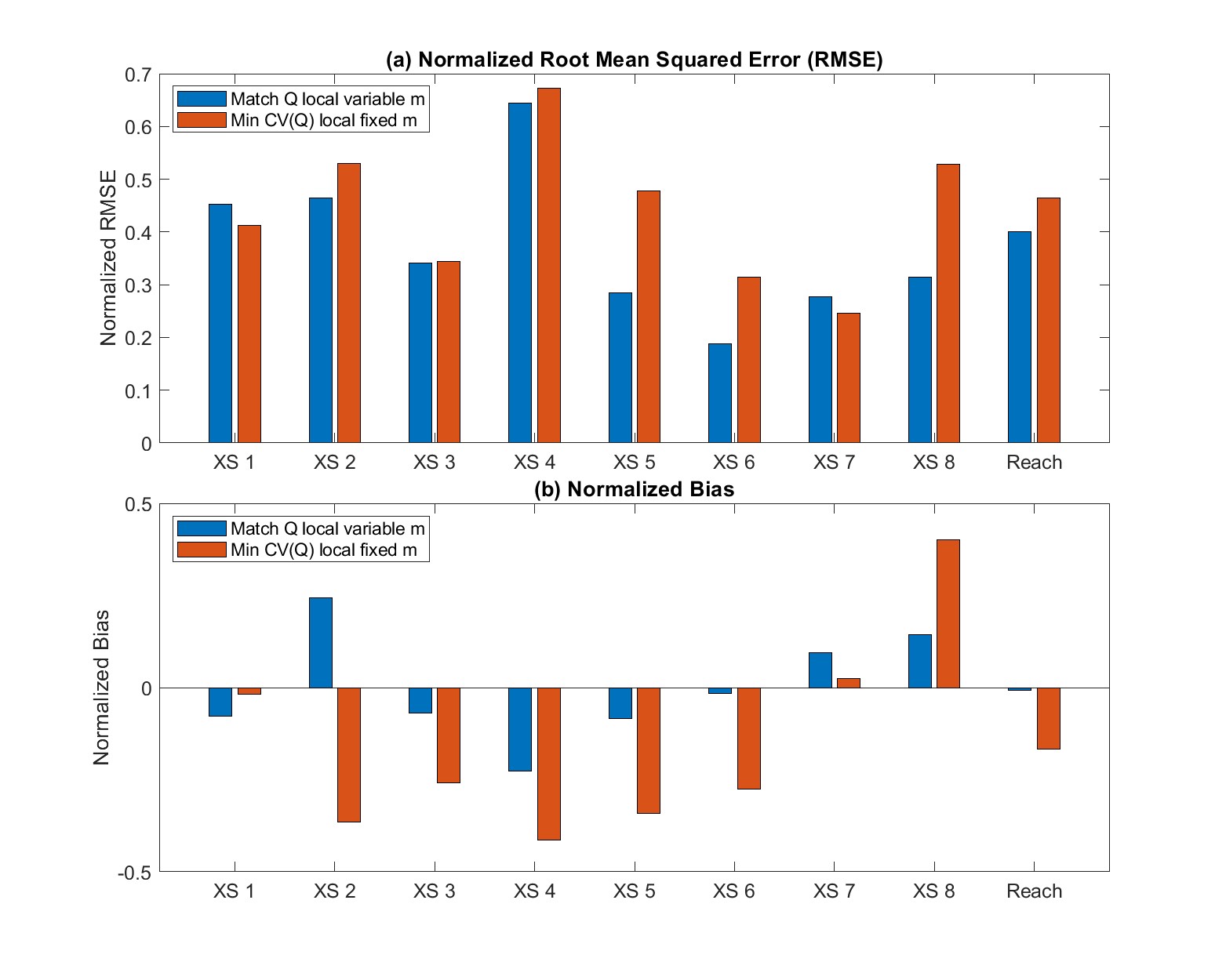
Accuracy assessment of output from the Depths Inferred from Velocities Estimated via Remote Sensing (DIVERS) framework designed to match a known discharge or minimize the coefficient of variation of estimated discharges, abbreviated min CV(Q), with power law velocity profile exponent m either variable or fixed. The (a) normalized root mean squared error (RMSE) and (b) normalized bias relative to depths measured in the field are used as metrics of performance and are plotted for each of the eight XSs surveyed along the Tanana River and for the reach-aggregated data set.
3.3. Sensitivity of DIVERS to initial estimates of parameters and uncertainties in input variables
To better understand the optimization process that ultimately led to the depth estimates shown in Figures 7 and 8, we performed a sensitivity analysis as described in Section 2.7. The effects of changes in each of the three potentially adjustable parameters (a, m, and k) and two input variables (us and S) on depths calculated via Equation 4 are illustrated in the top row of Figure 11, where the thin dashed lines indicate base case values. The bottom row shows the corresponding incremental changes in depth, calculated using the partial derivatives given by Equations 10 - 14. Examining these plots allowed us to interpret how depth estimates were influenced by each quantity. For example, values of a less than a0 led to larger predicted depths while values greater than a0 led to shallower depths. H was thus inversely related to a across this entire range, leading to the negative values of ∆H plotted in the bottom row. The slope became gentler for larger values of a, implying that a given change in a led to a smaller reduction in H as a approached 2a0. Mathematically, the decrease in H associated with an increase in a is a consequence of a appearing in the denominator of Equation 4. Physically, this inverse relationship reflects the increase in depth-averaged velocity that results from an increase in a (while the surface velocity remains fixed), which leads to a shallower depth for a given volume of water to convey.
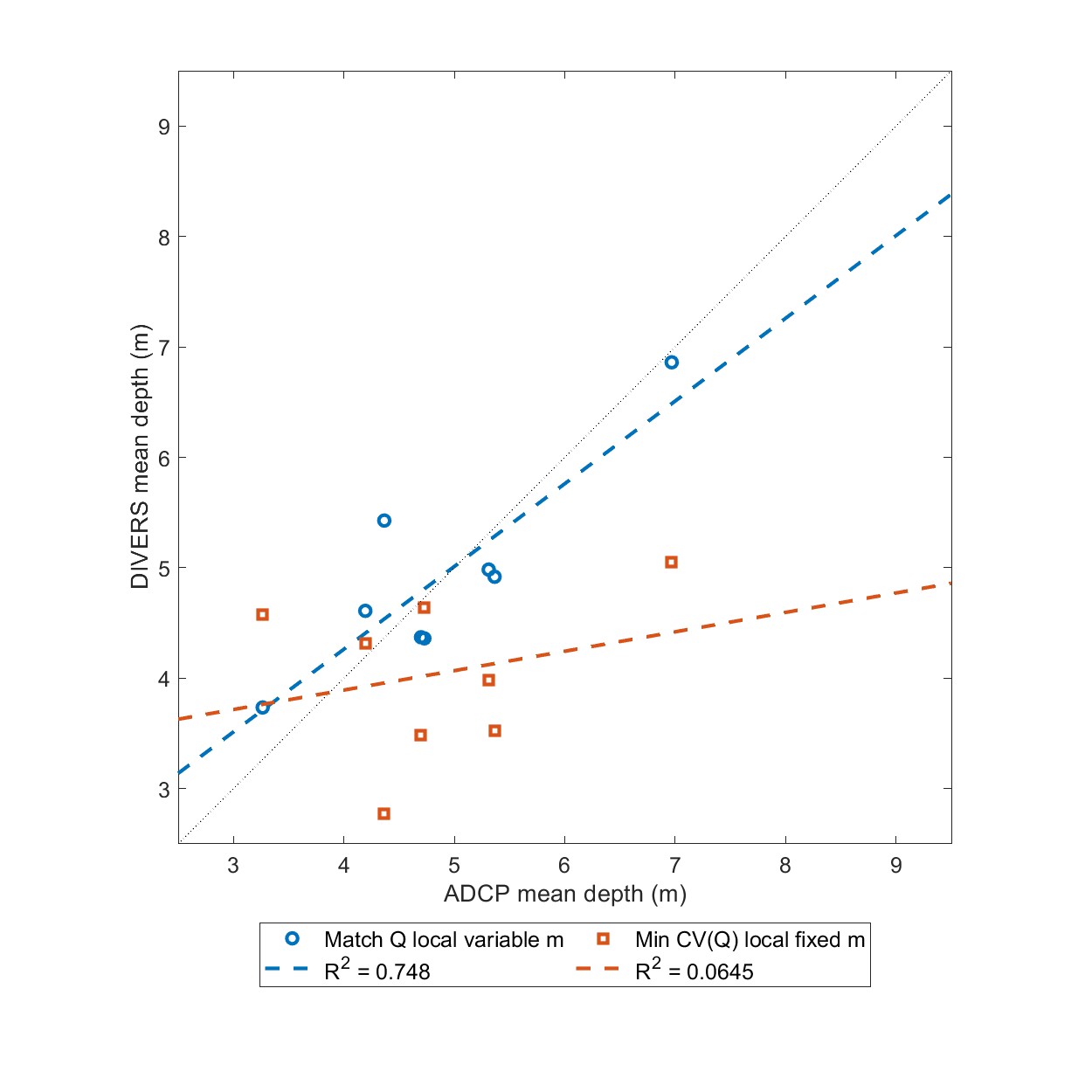
Accuracy assessment of output from the Depths Inferred from Velocities Estimated via Remote Sensing (DIVERS) framework designed to match a known discharge or minimize the coefficient of variation of estimated discharges, abbreviated min CV(Q), with the power law velocity profile exponent m either variable or fixed. The cross-sectional mean depths measured in the field with an acoustic Doppler current profiler (ADCP) are compared to the cross-sectional mean depths estimated via each variant of DIVERS by performing observed (ADCP) vs. predicted (DIVERS) regression. The R2 values for each regression are indicated in the legend and the 1-to-1 line of perfect agreement is shown with a thin, dotted black line for reference.
In general, conservation of mass dictates that under steady flow conditions any change that leads to a greater depth-averaged velocity will result in a shallower depth. Conversely, any reduction in depth-averaged velocity will be compensated for by an increase in depth. This reasoning implies that, for a given image-derived surface velocity, as the exponent m on the power law velocity profile increases, the depth-averaged velocity becomes greater and the depth shallower even though mass conservation is not explicitly enforced as part of the DIVERS workflow. The m values we considered correspond to α values from 0.799 to 0.941, within the range reported in the literature (e.g., Biggs et al., 2023) and representing velocity profile shapes varying from quite gentle to very steep. For the ADCP XSs from the Tanana River, α values ranged from 0.841 to 0.917 (LE23 supporting information). In addition, a previous study of the same reach found no evidence of unusual velocity profile shapes, such as a surface dip (refer to Figure 2 of Legleiter and Kinzel, 2021b). The roughness length scale k had the opposite effect on H, with larger values of k associated with greater depths such that ∆H was positive across the entire range from 0.5k0 to 2k0. This parameter appears in the numerator of Equation 4 and H is directly proportional to k because an increase in flow resistance leads to a decrease in depth-averaged velocity and thus an increase in depth for a given surface velocity.
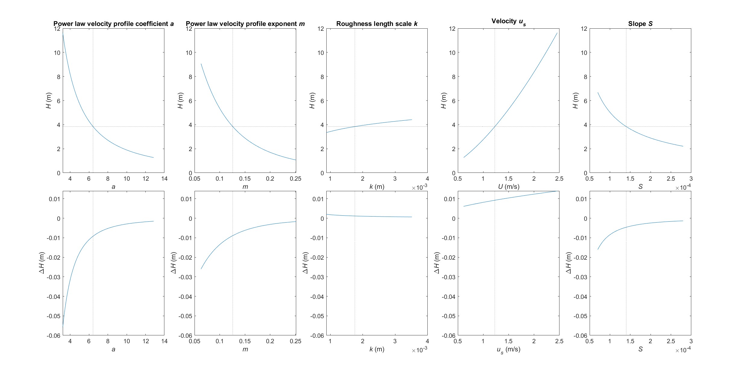
Sensitivity of depths calculated via Equation 4 to each of the variables appearing in that expression. Each column of this figure corresponds to one of these variables. The plots in the top row show how the absolute depth H varies as a function of each variable while the bottom row shows the incremental change in depth ∆H.
Similar logic can also be used to explain the impact of changes in the input variables on predicted depths. The fundamental premise of DIVERS is that depths can be inferred from image-derived surface velocities. Depth is directly related to surface velocity via Equation 4, with us raised to the power of 1/(0.5 + m) such that H increases non-linearly with us. The water surface slope S appears in the denominator of Equation 4 and is thus inversely related to H, as reflected by the negative values of ∆H shown in the last panel of Figure 11. The underlying physical process is that, for a given roughness (which we assume to be independent of slope), a steeper slope strengthens the gravitational force driving the water downstream, which leads to a higher velocity and thus a shallower depth.
Although Figure 11 provided some insight as to how depths estimated via DIVERS would be affected by changes in a, m, k, us, and S, these quantities had disparate units and led to changes in H that varied in magnitude. These differences made it difficult to assess which had the greatest impact on predicted depths. To clarify the relative influence of the parameters and input variables, we scaled each quantity by its base case value and divided H and ∆H by H0. The results of this analysis are summarized in Figure 12, which yielded greater insight as to the sensitivity of predicted depths to a, m, k, us, and S. Overall, us had the strongest influence on H, with a doubling of us leading to a three-fold increase in H whereas halving us would reduce H by a factor of approximately 2/3. Conversely, the roughness length scale had very little effect on depth, with H changing by less than 15% relative to its base case value as k increased from 0.5k0 to 2k0, although k might vary over a broader range if the bed material consists of poorly sorted sediment, which was not the case on the Tanana River (Toniolo, 2013). The other three quantities were all directly proportional to velocity and thus inversely proportional to depth, but the influence of S on H was less pronounced than that of a and m because only the latter two parameters affect the shape of the velocity profile. Whereas halving the slope led to a 73% increase in depth, the same reduction in a and m caused H to increase by factors of 2.36 and 3, respectively. Doubling a, m, and S relative to their base case values had less of an effect, leading to deceases in H of 43%, 67%, and 72%, respectively.
Figure 12b also shows that the incremental changes in depth relative to the base case depth, denoted, ∆H/H0, were greatest for the smallest values of a, m, and S relative to a0, m0, and S0. These results imply that the sensitivity of depth estimates to changes in these quantities was greatest when they were much less than their base case values, approaching half. Conversely, when a, m, and S were greater than their base case values, the incremental changes in depth were smaller in magnitude. In the context of the optimization algorithm, these results imply that increasing a and/or m from one iteration to the next would lead to smaller depths and therefore discharges, whereas decreasing either or both of these parameters would increase depth and discharge. Adjusting k, in contrast, would provide very little leverage in seeking to match a known discharge or minimize the coefficient of variation of estimated discharges. This finding is physically reasonable because the roughness length scale k is much less than the flow depth: H ≫ k. However, the 0.5k0 to 2k0 range we considered might not have been broad enough to accurately represent streambeds with a mix of fine and coarse sediment. In addition, bedforms and other types of form drag could also contribute to flow resistance and make k a more influential parameter.
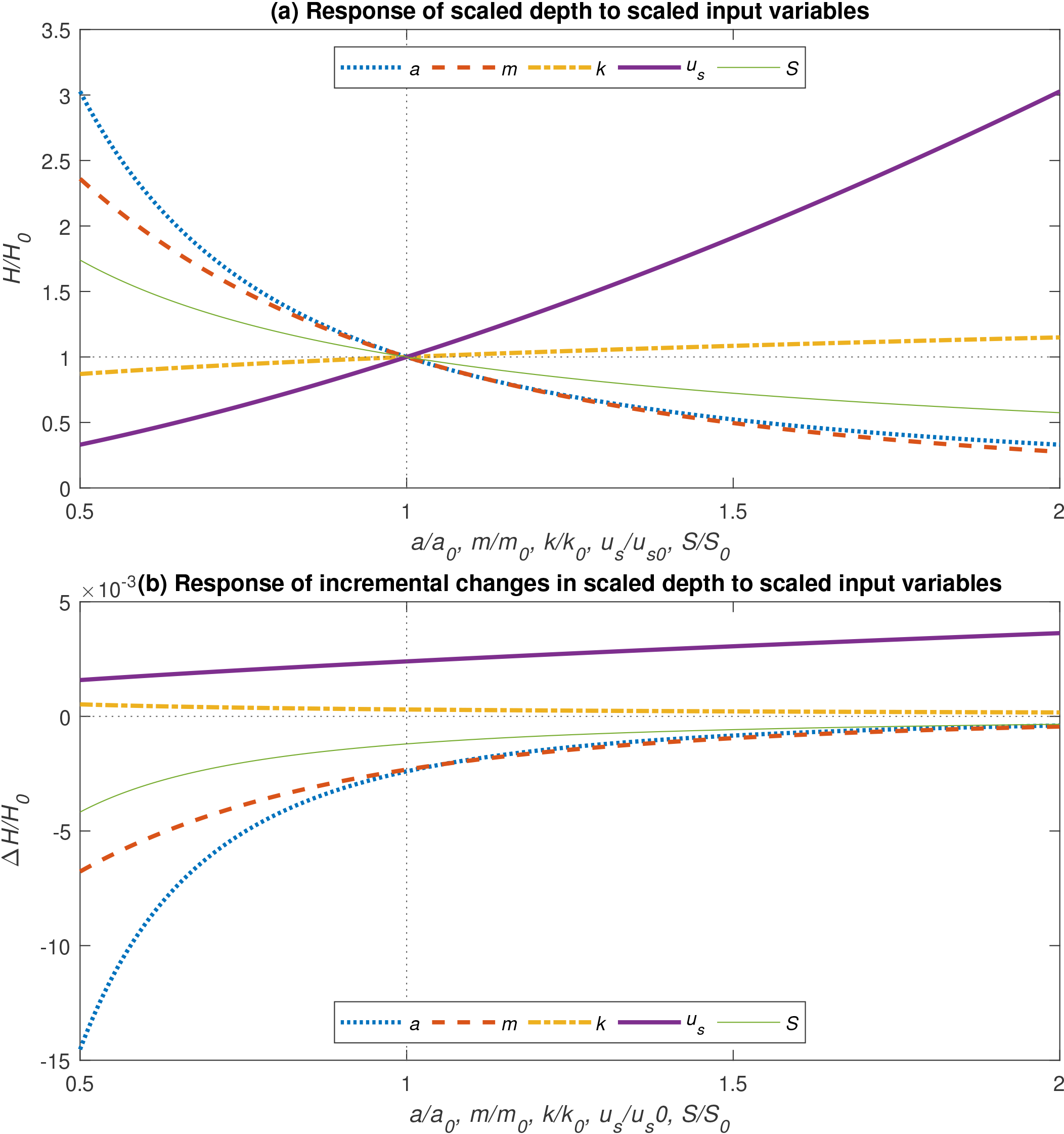
Sensitivity of calculated depths to each variable in Equation 4 expressed in non-dimensional form as described in the text. (a) Variations in scaled depth H/H0 as a function of each scaled input variable. (b) Variations in the incremental change in scaled depth ∆H/H0 as a function of each scaled input variable.
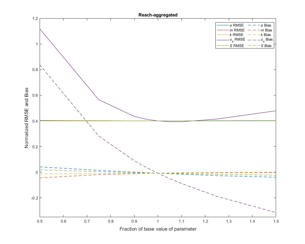
This analysis also implied that the output from the optimization algorithm might be sensitive to the initial estimates of a, m, and k and/or to errors in us and S. To investigate this possibility, we focused on the DIVERS implementation that led to the most accurate depth estimates: matching a known discharge while allowing m to vary. We performed a total of 45 runs with this variant, one for each of nine different values of each of the five inputs: 0.5, 0.75, 0.9, 0.95, 1, 1.05, 1.1, 1.25, and 1.5 times the base case values listed in Table 2. For each run, we calculated metrics of performance for each of the eight XSs surveyed in the field and for the reach-aggregated data set. The results of this analysis are summarized in Figure 13, where the normalized RMSE (solid lines) and mean bias (dashed lines) are plotted as a function of the fraction of the base case value of each of the input variables, which are distinguished by line color. Changing the initial estimates of the power law velocity profile parameters had essentially no impact on the normalized RMSE or mean bias. Similarly, an error in the water surface slope did not affect either of these metrics. The only quantity in Equation 4 that had any meaningful influence on the accuracy and precision of depth estimates was the surface velocity field. Providing a us smaller than its base case value as input led to greater normalized RMSEs, as much as 1.12 when us was only half its base case value. Using input velocity fields that were higher than the base case had less of an impact, with a normalized RMSE of 0.48 for a us twice as large as the base case. Because depth and surface velocity are directly related by Equation 4, the normalized mean bias was larger and more positive when us was smaller than its base case value, implying that depths were overpredicted when the input us was too low, up to 83% when us was half the base case. Conversely, the mean bias became increasingly negative for us inputs greater than the base case because depths were underpredicted, with a normalized mean bias of -31% when us was twice the base case. These results imply that depths estimated via this DIVERS variant were robust to misspecification of the power law velocity profile parameters and the water surface slope but were much more sensitive to errors in the input velocity field. Obtaining reliable depth estimates from an image-derived velocity field requires that this surface velocity field be highly accurate.
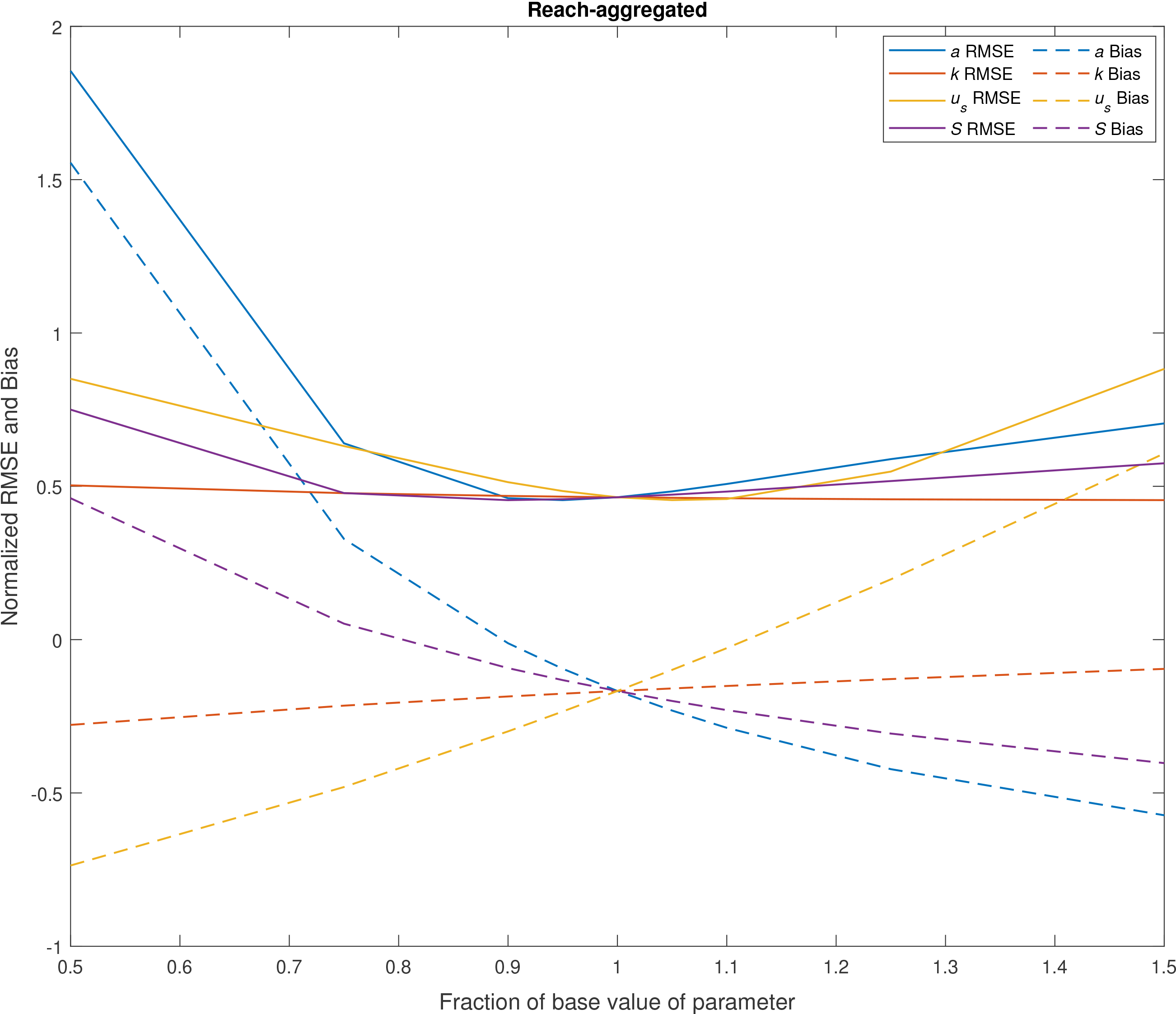
We also performed a similar analysis for the scenario where the discharge is not known a priori and the optimization algorithm instead seeks to minimize the coefficient of variation of estimated discharges by adjusting a and k. For this assessment, we performed a total of 36 runs, one for each of the nine different multipliers on the base case values used before but now for only four quantities because m was held fixed. The results summarized in Figure 14 indicate that the precision of depths inferred via DIVERS was more sensitive to initial parameter estimates when a known discharge was not available to serve as a constraint. Whereas only us had an appreciable impact on the normalized RMSE for fmQ, a also had a substantial effect when the optimization was based on fCVQ. For example, specifying an initial guess for a that was only 0.5a0 led to a normalized RMSE of 1.85 for the reach-aggregated data set, relative to a normalized RMSE of 0.46 for a0. Similarly, whereas only errors in us led to noticeable changes in normalized mean bias when seeking to match a known Q, a and S also influenced the magnitude of the bias when the objective was to minimize fCVQ. More specifically, providing an initial estimate of a that was too low (0.5a0) led to a normalized mean bias of 1.55 for the reach-aggregated data set while using an a that was too high (1.5a0) led to a normalized mean bias of -0.57; for the base case value of a0, the bias was -0.17. Larger values of a lead to higher velocities and therefore underpredictions of depth (i.e., a negative bias) when a is too high, and vice versa when a is too low. The water surface slope is also directly proportional to velocity and so had a similar but less pronounced effect on the normalized mean bias as a. For the input velocity field, using us smaller than the base case led to underpredictions of depth (i.e., a negative bias) and conversely when us was larger than the base case. This analysis suggests that although the precision of depth estimates produced by DIVERS when discharge is not known is fairly robust to misspecification of the input parameters and errors in the velocity field and water surface slope, the bias is much more sensitive to the values of a, us, and S used as input to the optimization algorithm.
Sensitivity of normalized root mean squared error (RMSE) and bias to variations in initial values of the parameters a, m, and k provided as input to the optimization algorithm for the discharge matching, variable m variant. Note that the solid, colored lines all overlap one another except for that representing the surface velocity us.
We also assessed how discharge estimates would be affected by misspecification of a and k and errors in us and S. To do so, we calculated the mean of the estimated discharges resulting from each of the 36 sensitivity analysis runs and plotted them as a function of each input quantity in Figure 15a-d. Varying the value of a provided as input from 0.5a0 to 1.5a0 led to discharges ranging from 3,821 m3/s to 660 m3/s relative to a base case value of 1,258 m3/s. The roughness length scale had less of an impact, as expected given the results summarized in Figure 12 (and the fact that H ≫ k), but the mean estimated discharge still increased appreciably as we increased k from0.5 to 1.5 times its base case value. As dictated by Equation 4, using a surface velocity field that was too small led to major underpredictions of discharge whereas systematically overestimating the velocity would translate into overpredictions of discharge. Errors in water surface slope were inversely related to the mean estimated discharge, suggesting that the increase in depth associated with a decrease in slope outweighed the corresponding decrease in velocity and vice versa for an increase in slope.
Sensitivity of normalized root mean squared error (RMSE) and bias to variations in initial values of the power law velocity profile parameters a and k, velocity us, and slope S provided as input to the coefficient of variation of estimated discharges-minimizing, fixed m variant.
The impacts of these four quantities on the mean of the estimated discharges are difficult to compare because a, k, us, and S have different units. To better understand the degree to which each input affected the estimated discharges, we expressed these results in non-dimensional form by expressing each quantity as a fraction of its base case value and scaling the discharge estimates by the known discharge, which was not used for optimization based on fCVQ. The results of this analysis are shown in Figure 15e. Both the velocity profile coefficient a and image-derived velocity field us had strong effects on the estimated discharge but in opposite directions. Halving a led to a 2.74-fold increase in discharge whereas using us values that were 50% too large caused the mean estimated discharge to increase by a factor of 2.6. Errors in water surface slope had a modest effect, with the mean estimated discharge decreasing from 1.57 to 0.65 times the known discharge as S increased from 0.5 to 1.5 times its base case value. The roughness length scale k had the least impact on the estimated discharge, with the mean discharge varying from 0.78 to 0.98 times the known discharge as k was varied from 0.5k0 to 1.5k0. As mentioned previously, the influence of roughness might be greater if a broader range of k were considered. This analysis suggests that the close agreement between the mean of the discharges estimated via DIVERS when using fCVQ as the objective function (1,258 m3/s) and the known discharge (1,393 m3/s) was largely the result of fortuitous initial estimates of a and k and accurate inputs for us and S. However, had these estimates been farther off or had the surface velocity and slope measurements been less reliable, the estimated discharges likely would have been much less accurate. For this reason, the DIVERS framework is better-suited to situations where a known discharge is available to constrain the optimization algorithm.
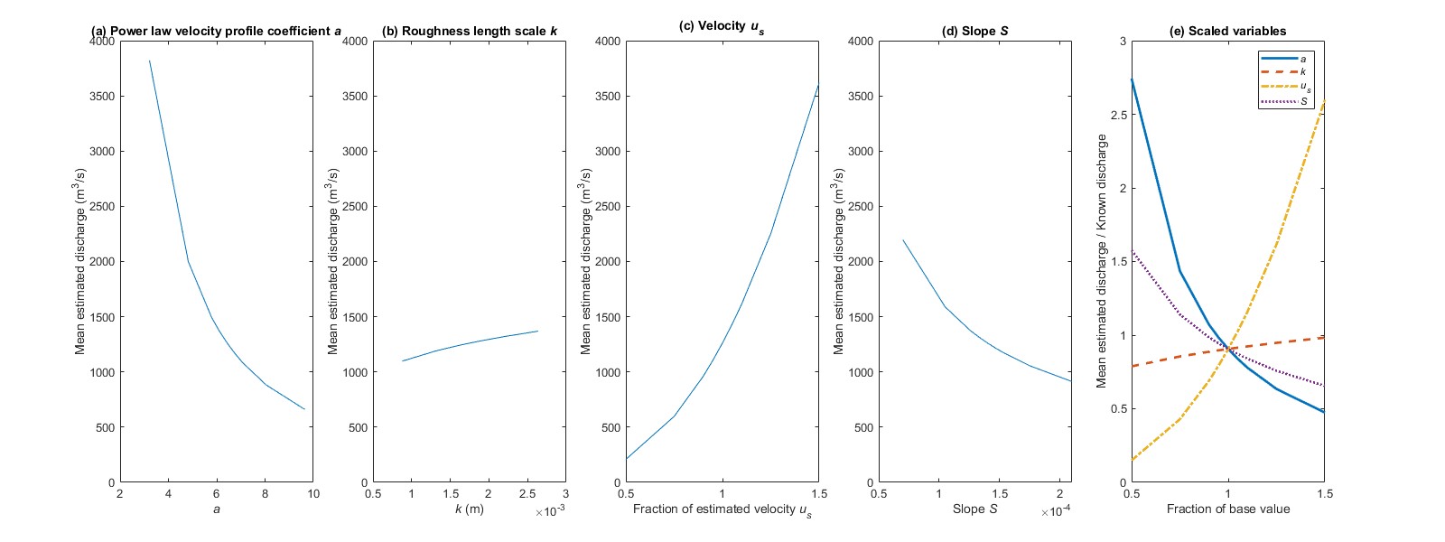
Sensitivity of estimated discharge to variations in initial values of (a) power law velocity profile coefficient a, (b) roughness length scale (k), (c) velocity us, and (d) slope S provided as input to the coefficient of variation of estimated discharges-minimizing, fixed m version of DIVERS. (e) Comparison of scaled input variables obtained by dividing each by its base case value and scaling the mean estimated discharges by the known discharge.
4. Discussion
4.1. Effects of velocity profile shape on depth estimation via DIVERS
The foundation of the DIVERS framework is an expression relating the image-derived surface velocity us to depth H (Equation 4) given an assumed shape of the vertical velocity profile (Equation 2). The sensitivity analyses summarized in Section 3.3 quantified how variations in the coefficient a, exponent m, and roughness length scale k affect depths estimated via DIVERS. Here, we link these results back to the shape of the velocity profile to provide a plausible physical explanation for our findings.
Our interpretation is based upon Figure 16, the top row of which shows how the velocity profile changes as one parameter varies while the other two are held fixed. To generalize this analysis, each parameter is scaled by its base case value from Table 2 and varied from half to 1.5 times the base value. The vertical scale of the velocity profiles is non-dimensionalized by dividing the height z above the bed by the total flow depth H. Values of a less than a0 lead to smaller velocities at a given vertical position within the water column and a steeper profile shape such that velocity varies less from the bed to the water surface. In contrast, for a > a0 the velocities become greater and the profile flattens as a increases. Because DIVERS is based on remotely sensed surface velocities, a value of a that is too large is equivalent to observing a greater velocity at the water surface. Figure 16b shows that m has a similar effect, with m < m0 leading to lower velocities at a given height above the bed and a steeper profile shape, whereas values of m larger than m0 yield higher velocities and flatter profiles; this effect becomes more pronounced as m approaches 1.5m0. Variations in the roughness length scale have a relatively minor impact on velocities throughout the water column and negligible influence on the shape of the profile (Figure 16c).
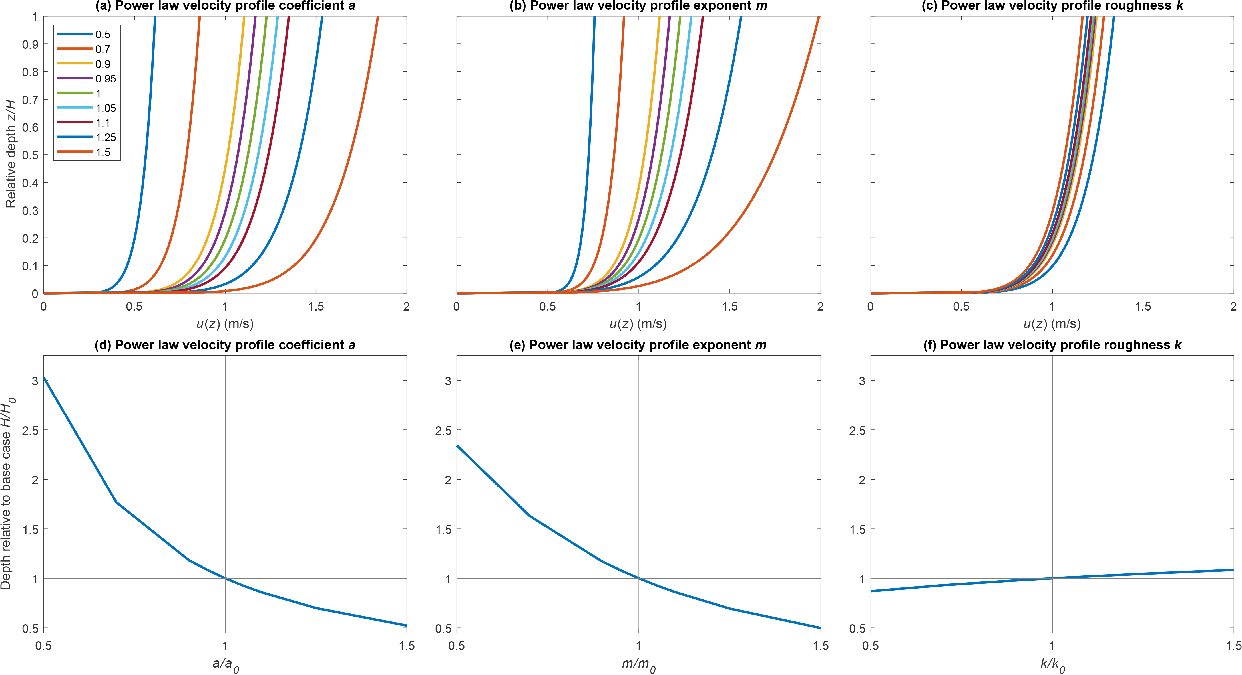
Effects of the three parameters in Equation 2 on (a-c) the shape of the vertical velocity profile and (d-f) depths inferred from remotely sensed surface velocities.
The bottom row of Figure 16 illustrates how these changes propagate through Equation 4 to influence depths estimated via DIVERS. This analysis is also presented in a non-dimensional form, with the depths scaled by the base case value H0 calculated from Equation 4 using the reach-averaged us from the MARV output and the values of a0, m0, and k0 listed in Table 2. Figure 16d shows that depths are over-predicted when a < a0 by a factor of up to three relative to H0 when a = 0.5a0. If a is too low, the vertical profile would have to extend upward through a much deeper water column in order for u(z = H) to match the observed us, resulting in a substantial overprediction of depth. Conversely, if a is larger than a0, depths are under-predicted by a factor of nearly two for a = 1.5a0. If a is too high, the velocity profile does not have to extend through as thick a water column before reaching the depth at which u(z = H) = us, so depths are underestimated. Because the effect of m on the vertical velocity profile is similar to that of a, the same line of reasoning also pertains to Figure 16e: if m is too small, depths will be over-predicted, whereas using an m that is too large will lead to underestimates of depth. The effect of roughness is again relatively minor, with k < k0 leading to slight underpredictions of depth while k > k0 causes depths to be overestimated by a small amount (Figure 16f).
4.2. Persistent assumptions and limitations of the DIVERS framework
The DIVERS framework is built upon a number of critical, simplifying assumptions. The foundation of the entire workflow is a basic flow resistance equation that links velocity to depth under the assumption of steady, uniform, one-dimensional flow; any flux of mass or momentum in the vertical or cross-stream directions is neglected. Although we treat the flow as fully turbulent, with a boundary layer that extends throughout the entire depth, we use a mathematically convenient power law formulation of the vertical velocity profile. A more rigorous approach might use a logarithmic velocity profile associated with a parabolic vertical distribution of eddy viscosity. By using the water surface slope in place of the pressure gradient, we also assume that the flow is hydrostatic (Nelson et al., 2003).
The most important assumption we make is the essence of DIVERS: a flow resistance equation intended for characterizing the bulk, one-dimensional hydraulics of a channel cross section can be applied to calculate local flow depths. Invoking this approximation allows estimated depths to vary laterally across the channel from one node of a grid of image-derived surface velocities to the next. However, each of these nodes is essentially an isolated water column independent of those around it, with no information transferred from upstream, downstream, or either side. An important implication is that secondary flows involving cross-stream currents, as occur in meander bends, are not taken into account. This issue is particularly acute in areas of recirculating flow (i.e., eddies), which must be omitted because negative streamwise velocities are incompatible with Equation 4. The assumptions inherent to DIVERS also dictate that the depth at a given location is influenced only by the image-derived surface velocity at that location and is strictly proportional to that velocity. As a result, areas where the flow becomes shallower but also faster, as along the margins of a point bar, or deepens but slows, as in a pool, cannot be captured by this approach.
The DIVERS framework thus offers, at best, a basic, first-order approximation to the actual hydraulic conditions present within the channel of interest. As presently formulated, DIVERS does not allow for more complex flow patterns that do not conform to the assumptions upon which the workflow is based. Although the refinements introduced in this study provide greater flexibility than LK21, DIVERS is still best-suited to situations where the flow is relatively simple and the underlying assumptions are not egregiously inappropriate. These conditions are more likely to be satisfied in rivers with a straight, uniform morphology when the discharge is close to bankfull. For example, in this study the strongest agreement between observed and predicted depths occurred at XS 2, 3, 6, and 7 (Figure 8), which were located in straight portions of the reach where the assumptions underlying DIVERS were most likely to be valid. Conversely, DIVERS becomes more tenuous in more complex and/or highly sinuous channels, particularly at lower discharges when convective accelerations might be important (Whiting and Dietrich, 1991; Whiting, 1997). Although our results suggest that DIVERS can provide plausible depth estimates under certain conditions, further testing across a broader range of river environments is needed to better understand where and when this approach can yield reliable bathymetry.
4.3. Potential for reach-scale mapping of multiple river attributes
Although these limitations are meaningful and must be kept in mind, the generalized DIVERS framework could advance our ability to characterize rivers via remote sensing. More specifically, inferring depth from velocity could enable bathymetric mapping in rivers that are too turbid or deep for spectrally based depth retrieval or lidar. A reach-scale depth map like that generated via DIVERS (Figure 17) could not have been produced by applying more established remote sensing techniques to this large, sediment-laden river. An improved capacity to efficiently measure water depth in river channels would be valuable because channel geometry is a key input to hydraulic models used to predict flood inundation (e.g., Grimaldi et al., 2018), assess habitat suitability (e.g., Harrison et al., 2022), and route sediment, nutrients, and contaminants along river networks (e.g., Wiele et al., 2007). Many of these applications would also require information on water surface elevations, but such data potentially could be derived from the same sequence of images used for velocity estimation via photogrammetry or structure-from-motion techniques (e.g., Fonstad et al., 2013). This approach would ensure that the DIVERS calculations are based upon velocities and water surface slopes measured simultaneously, which would avoid the uncertainty that might be introduced by a time gap between the two types of observations.
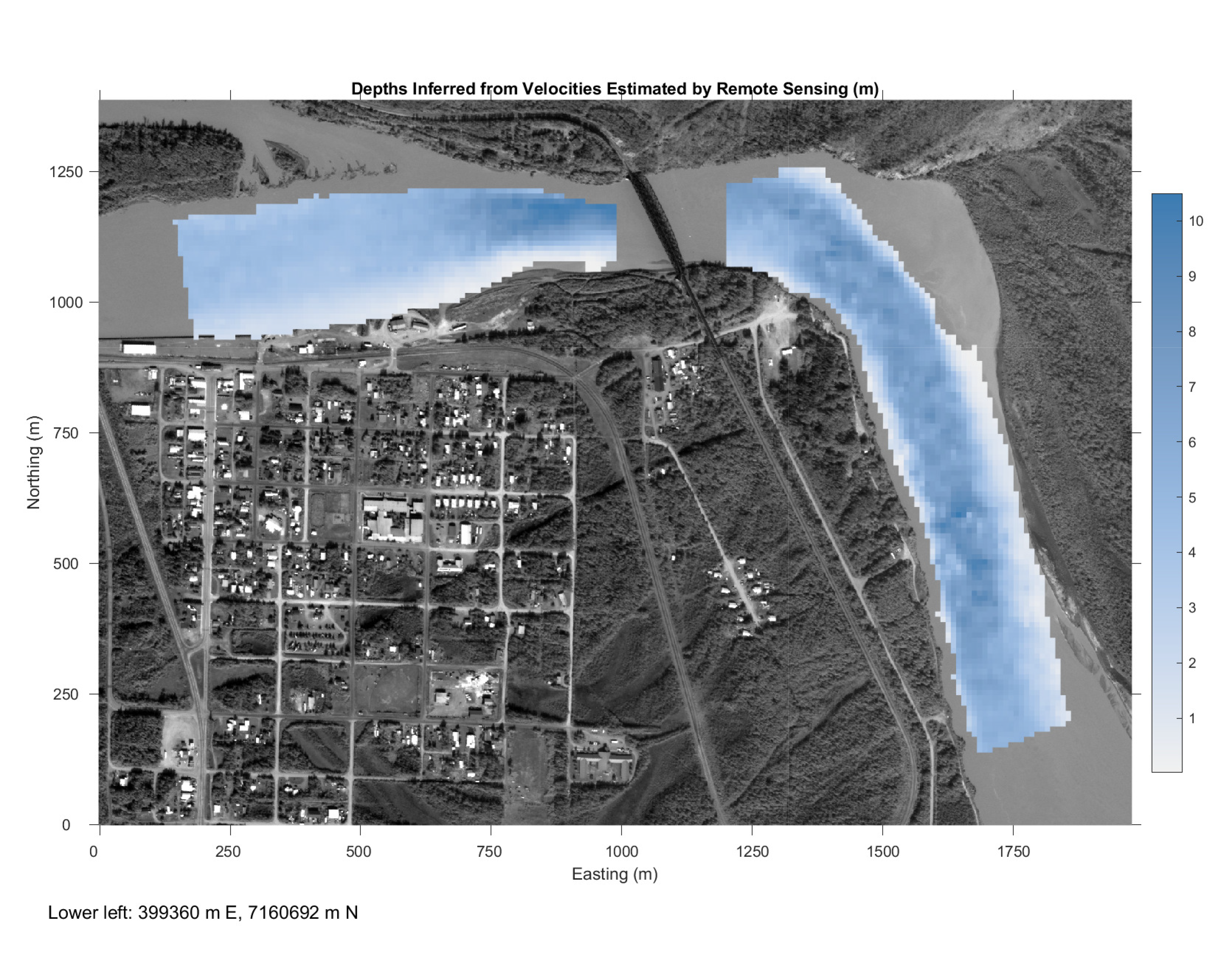
Final depth map produced using the discharge-matching, variable m version of DIVERS and back-transformed to the original spatial coordinate system.
The DIVERS framework is consistent with broader efforts by the hydrologic remote sensing community to measure river discharge via remote sensing, most notably through the Surface Water and Ocean Topography (SWOT) mission (Biancamaria et al., 2016), although the results of this study suggest that depths inferred via DIVERS are more likely to be accurate when discharge is known a priori and can be provided as an input. As described by Durand et al. (2023), numerous approaches have been developed to estimate discharge using SWOT observations of water surface elevation, width, and slope. However, these techniques also must make assumptions regarding certain quantities not measured by SWOT, including bathymetry. DIVERS is analogous to the various SWOT discharge algorithms in the sense that river attributes that can be measured, such as velocity in the case of DIVERS or water surface elevation in the case of SWOT, must be combined with hydraulic principles to infer other quantities, such as depth, that cannot be observed directly. Exploring potential synergies between the optimization-based approach used in DIVERS and SWOT workflows could foster progress toward an operational capacity for remote sensing of discharge.
Further investigation of several other topics could also enhance the utility of DIVERS. For example, our case study focused on a reach immediately adjacent to an established gaging station, so the discharge at the time of image acquisition could be used to constrain the optimization. Although we presented a second objective function, fCVQ, that does not require a priori knowledge of discharge, the discharge-matching approach provided closer results to those observed in the field. Identifying different sources of discharge information could thus expand the applicability of DIVERS. For example, an inverse approach could be used to infer water depth, and thus discharge, from measurements of velocity and water surface slope (e.g., Zaron et al., 2011; Nelson et al., 2012). Large-scale hydrologic models can provide discharge estimates with high spatial and temporal resolution, particularly when assimilated with remotely sensed data (e.g., Feng et al., 2021), and could provide an alternative to streamgages. Similarly, we used a lidar DEM to measure water surface slope along the Tanana River, but such data are rare; incorporating more common topographic data would increase the applicability of the approach. For example, the SWOT mission was designed to accurately measure water surface elevations in rivers more than 100 m wide and a database for this information has been established (Altenau et al., 2021). In the U.S., the National Hydrography Dataset includes reach slopes calculated from the best available topographic data (Moore et al., 2019).
5. Conclusion
The difficulty and expense of measuring velocity, depth, and discharge directly in the field makes remote sensing of rivers an appealing alternative. Recent advances in image velocimetry have created new possibilities for large-scale mapping of hydraulic conditions and could form the basis of a non-contact streamgaging approach. However, estimating the other variable required to calculate discharge, water depth, from remotely sensed data remains challenging in large, turbid rivers. The Depths Inferred from Velocities Estimated via Remote Sensing (DIVERS) framework addresses this issue by capitalizing upon our ability to derive velocities from image time series to calculate depths indirectly via an expression that relates depth to surface velocity for an assumed power law velocity profile.
In this study, we generalized the DIVERS workflow in several ways. Rather than a patchwork of velocity fields obtained by hovering at a series of distinct locations, we used images acquired from a moving aircraft to obtain more extensive, continuous spatial coverage. Transforming the resulting velocity field to a channel-centered coordinate system allowed us to isolate streamwise velocity vector components and facilitated hydraulic calculations. We modified the optimization algorithm by allowing for multiple free parameters and local calibration on a per-cross section basis. Introducing a second objective function to minimize the coefficient of variation of estimated discharges along a reach enabled the approach to be applied in cases where the discharge is not known a priori. We also performed a sensitivity analysis to gain insight as to which quantities had the greatest impact on depth estimates and to assess robustness to misspecification of initial parameter estimates and errors in input variables.
The results of this study support the following principal conclusions:
-
1. Moving aircraft river velocimetry (MARV) provides a more efficient means of mapping long river segments and led to velocity estimates that were more accurate than those based on data acquired from a helicopter. In this case study, MARV led to strong agreement (R2 = 0.81) between image-derived velocities and field measurements.
-
2. Two variants of DIVERS distinguished by which parameters were allowed to vary and whether the objective was to match a known discharge or minimize the coefficient of variation of estimated discharges were tested. The version that led to the most accurate depth estimates allowed the power law velocity profile exponent m to vary during a local optimization to match the known discharge. Comparison of cross-sectional mean depths inferred via this DIVERS variant to those measured in the field led to an R2 of 0.75. This result implies that if the discharge is known a priori, DIVERS can provide accurate cross-sectional mean depths without having to impose a specific value of a parameter (m) that describes the shape of the velocity profile.
-
3. The sensitivity of depth estimates to each of the five quantities in the flow resistance equation used to calculate depths from image-derived surface velocities varied widely, with velocity having the greatest impact on depth and the roughness length scale having the least. The water surface slope and the coefficient and exponent of the power law velocity profile were inversely related to depth because an increase in any of these quantities led to an increase in velocity, such that a shallower depth was needed to convey a given volume of water.
-
4. Depths estimated via the DIVERS workflow were robust to misspecification of the power law velocity profile parameters and the water surface slope but were much more sensitive to errors in the input velocity field, with depths underpredicted when velocities were too low and overpredicted if the velocities were too high. For the variant based on minimizing the coefficient of variation of estimated discharges, depth estimates were also sensitive to the initial estimate of the velocity profile coefficient and to errors in water surface slope.
-
5. For this case study, minimizing the coefficient of variation of estimated discharges led to a discharge within 10% of that measured at a gaging station. However, sensitivity analysis indicated that this result was a consequence of fortuitous initial parameter estimates and that discharges inferred via this approach were highly sensitive to misspecification of these parameters and to errors in the velocity field and, to a lesser degree, water surface slope provided as input. DIVERS is thus better-suited to situations where a known discharge is available.
-
6. Although the refinements to the DIVERS framework presented in this study provide greater flexibility, the approach is still based on a number of simplifying assumptions that limit its applicability and performance, particularly in smaller, more complex channels at lower flows. DIVERS is predicated upon an assumption of steady, uniform, one-dimensional flow and neglects any cross-stream transfer of mass or momentum. In addition, because a flow resistance equation intended to characterize bulk, cross-sectionally averaged hydraulics is applied to each node of a grid of image-derived velocities, the depth estimated at a given location is strictly proportional to the velocity at that location. As presently formulated, DIVERS cannot capture more complex situations where the flow becomes shallower but also faster or deepens and slows.
-
7. These assumptions impose important limitations, but the results of this study provide further evidence that the DIVERS framework can provide plausible, first-order depth estimates in highly turbid rivers that cannot be mapped effectively via more established remote sensing techniques. Further testing across a broader range of river environments is needed to better understand where DIVERS can provide reliable bathymetric information. Additional research could also focus on relaxing some of the assumptions inherent to the current approach.
Acknowledgements
Jeff Conaway, Heather Best, and Elizabeth Richards of the USGS Alaska Science Center made field measurements of flow depth and velocity on the Tanana River. Mark Laker, Nate Olson, Brett Nigus, and Frances Nelson of the U.S. Fish and Wildlife Service (USFWS) coordinated flights and acquired images. Christina Leonard provided a valuable review of an earlier version of this paper. Any use of trade, firm, or product names is for descriptive purposes only and does not imply endorsement by the U.S. Government.
References
Altenau, E.H., Pavelsky, T.M., Durand, M.T., Yang, X., Prata de Moraes Frasson, R., Bendezu, L., Frasson, R.P.d.M., Bendezu, L., 2021. The Surface Water and Ocean Topography (SWOT) Mission River Database (SWORD): A Global River Network for Satellite Data Products. Water Resources Research 57, e2021WR030054. URL: https://doi.org/10.1029/2021WR030054.
Bandini, F., Kooij, L., Mortensen, B.K., Bauer-gottwein, P., 2023. Mapping inland water bathymetry with Ground Penetrating Radar (GPR) on board Unmanned Aerial Systems (UASs) . Journal of Hydrology 616, 128789. URL: https://doi.org/10.21203/rs.3.rs-877656/v1.
Biancamaria, S., Lettenmaier, D.P., Pavelsky, T.M., 2016. The SWOT Mission and Its Capabilities for Land Hydrology. Surveys in Geophysics 37, 307–337. URL: https://link.springer.com/article/10.1007/s10712-015-9346-y.
Biggs, H., Smart, G., Doyle, M., Eickelberg, N., Aberle, J., Randall, M., Detert, M., 2023. Surface Velocity to Depth-Averaged Velocity: A Review of Methods to Estimate Alpha and Remaining Challenges. Water 15, 3711. URL: https://doi.org/10.3390/w15213711.
Biggs, H.J., Smith, B., Detert, M., Sutton, H., 2022. Surface image velocimetry: Aerial tracer particle distribution system and techniques for reducing environmental noise with coloured tracer particles. River Research and Applications 38, 1192–1198. URL: https://doi.org/10.1002/rra.3973.
Bodart, G., Le Coz, J., Jodeau, M., Hauet, A., 2024. Quantifying and Reducing the Operator Effect in LSPIV Discharge Measurements. Water Resources Research 60, e2023WR034740. URL: https://doi.org/10.1029/2023WR034740.
Conaway, J., Eggleston, J., Legleiter, C., Jones, J., Kinzel, P., Fulton, J., 2019. Remote sensing of river flow in Alaska—New technology to improve safety and expand coverage of USGS streamgaging. U.S. Geological Survey Fact Sheet 2019, 4. URL: https://doi.org/10.3133/fs20193024.
Costa, J.E., Cheng, R.T., Haeni, F.P., Melcher, N., Spicer, K.R., Hayes, E., Plant, W., Hayes, K., Teague, C., Barrick, D., 2006. Use of radars to monitor stream discharge by noncontact methods. Water Resources Research 42, doi: https://doi.org/10.1029/2005WR004430.
Detert, M., Cao, L., Albayrak, I., 2019. Airborne Image Velocimetry Measurements at the Hydropower Plant Schiffmu¨hle on Limmat River, Switzerland, in: Proceedings of the 2nd International Symposium and Exhibition on Hydro-Environment Sensors and Software, HydroSenSoft 2019, IAHR, Madrid, Spain. pp. 211 – 217. URL: https://doi.org/10.3929/ethz-b-000341626.
Dolcetti, G., Hortoba’gyi, B., Perks, M., Tait, S.J., Dervilis, N., 2022. Using Noncontact Measurement of Water Surface Dynamics to Estimate River Discharge. Water Resources Research 58, e2022WR032829. URL: https://agupubs.onlinelibrary.wiley.com/doi/abs/10.1029/2022WR032829, doi: https://doi.org/10.1029/2022WR032829.
Durand, M., Gleason, C.J., Pavelsky, T.M., de Moraes Frasson, R., Turmon, M., David, C.H., Altenau, E.H., Tebaldi, N., Larnier, K., Monnier, J., Malaterre, P.O., Oubanas, H., Allen, G.H., Astifan, B., Brinkerhoff, C., Bates, P.D., Bjerklie, D., Coss, S., Dudley, R., Fenoglio, L., Garambois, P.A., Getirana, A., Lin, P., Margulis, S.A., Matte, P., Minear, J.T., Muhebwa, A., Pan, M., Peters, D., Riggs, R., Sikder, M.S., Simmons, T., Stuurman, C., Taneja, J., Tarpanelli, A., Schulze, K., Tourian, M.J., Wang, J., 2023. A Framework for Estimating Global River Discharge From the Surface Water and Ocean Topography Satellite Mission. Water Resources Research 59, e2021WR031614. URL: https://doi.org/10.1029/2021WR031614.
Eltner, A., Bertalan, L., Grundmann, J., Perks, M.T., Lotsari, E., 2021. Hydro-morphological mapping of river reaches using videos captured with UAS. Earth Surface Processes and Landforms 46, 2773–2787. URL: https://doi.org/10.1002/esp.5205.
Fediuk, A., Wunderlich, T., Wilken, D., Rabbel, W., 2022. Ground Penetrating Radar Measurements in Shallow Water Environments: A Case Study. Remote Sensing 14, 3659. URL: https://doi.org/10.3390/rs14153659.
Feng, D., Gleason, C.J., Lin, P., Yang, X., Pan, M., Ishitsuka, Y., 2021. Recent changes to Arctic river discharge. Nature Communications 12, 6917. URL: https://doi.org/10.1038/s41467-021-27228-1.
Ferguson, R., 2007. Flow resistance equations for gravel- and boulder-bed streams. Water Resources Research 43, W05427. URL: https://doi.org/10.1029/2006WR005422.
Fonstad, M.A., Dietrich, J.T., Courville, B.C., Jensen, J.L., Carbonneau, P.E., 2013. Topographic structure from motion: A new development in photogrammetric measurement. Earth Surface Processes and Landforms 38, 421–430. URL: https://doi.org/10.1002/esp.3366.
Grimaldi, S., Li, Y., Walker, J.P., Pauwels, V.R.N., 2018. Effective Representation of River Geometry in Hydraulic Flood Forecast Models. Water Resources Research 54, 1031–1057. URL: https://doi.org/10.1002/2017WR021765.
Harrison, L.R., Legleiter, C.J., Sridharan, V.K., Dudley, P.N., Daniels, M.E., 2022. Evaluating the Sensitivity of Multi-Dimensional Model Predictions of Salmon Habitat to the Source of Remotely Sensed River Bathymetry. Water Resources Research 58, e2022WR033097. URL: https://doi.org/10.1029/2022WR033097.
Johnson, E.D., Cowen, E.A., 2016. Remote Monitoring of Volumetric Discharge Employing Bathymetry Determined from Surface Turbulence Metrics. Water Resources Research 52, 2178–2193. doi: https://doi.org/10.1002/2015wr017736.
Lagarias, J.C., Reeds, J.A., Wright, M.H., Wright, P.E., 1998. Convergence Properties of the Nelder–Mead Simplex Method in Low Dimensions. SIAM Journal on Optimization 9, 112–147. URL: https://doi.org/10.1137/S1052623496303470.
Legleiter, C., 2024. TRiVIA - Toolbox for River Velocimetry using Images from Aircraft (ver. 2.1.3, September, 2024). URL: https://doi.org/10.5066/P9AD3VT3.
Legleiter, C., Harrison, L.R., 2019. Remote Sensing of River Bathymetry: Evaluating a Range of Sensors, Platforms, and Algorithms on the Upper Sacramento River, California, USA. Water Resources Research 55, 2142–2169. URL: https://doi.org/10.1029/2018WR023586.
Legleiter, C., Kinzel, P., 2021a. Depths Inferred from Velocities Estimated by Remote Sensing: A Flow Resistance Equation-Based Approach to Mapping Multiple River Attributes at the Reach Scale. Remote Sensing 13, 4566. URL: https://doi.org/10.3390/rs13224566.
Legleiter, C., Kinzel, P., Laker, M., Conaway, J., 2022. Digital orthophotos and field measurements of flow velocity from the Tanana and Nenana Rivers, Alaska, from August 2021 (ver. 2.0, June 2024). U.S. Geological Survey data release, https://doi.org/10.5066/P968OENT.
Legleiter, C., Kinzel, P.J., 2020. Inferring Surface Flow Velocities in Sediment-Laden Alaskan Rivers from Optical Image Sequences Acquired from a Helicopter. Remote Sensing 12, 1282. URL: https://doi.org/10.3390/rs12081282.
Legleiter, C.J., Kinzel, P.J., 2021b. Surface Flow Velocities From Space: Particle Image Velocimetry of Satellite Video of a Large, Sediment-Laden River. Frontiers in Water 3, 652213. URL: https://doi.org/10.3389/frwa.2021.652213.
Legleiter, C.J., Kinzel, P.J., 2023. The Toolbox for River Velocimetry using Images from Aircraft (TRiVIA). River Research and Applications 39, 1457–1468. URL: https://doi.org/10.1002/rra.4147.
Legleiter, C.J., Kinzel, P.J., 2024a. A framework to facilitate development and testing of image-based river velocimetry algorithms. Earth Surface Processes and Landforms 49, 1361–1382. URL: https://doi.org/10.1002/esp.5772.
Legleiter, C.J., Kinzel, P.J., 2024b. An enhanced and expanded Toolbox for River Velocimetry using Images from Aircraft (TRiVIA). River Research and Applications, https://doi.org/10.1002/rra.4333URL: 10.1002/rra.4333.
Legleiter, C.J., Kinzel, P.J., Laker, M., Conaway, J.S., 2023. Moving Aircraft River Velocimetry (MARV): Framework and Proof-of-Concept on the Tanana River. Water Resources Research 59, e2022WR033822. URL: https://doi.org/10.1029/2022WR033822.
Legleiter, C.J., Kyriakidis, P.C., 2006. Forward and inverse transformations between Cartesian and channel-fitted coordinate systems for meandering rivers. Mathematical Geology 38, 927–958. URL: https://doi.org/10.1007/s11004-006-9056-6.
Ljubičić, R., Dal Sasso, S.F., Zindović, B., 2024. SSIMS-Flow: Image velocimetry workbench for open-channel flow rate estimation. Environmental Modelling & Software 173, 105938. URL: https://doi.org/10.1016/j.envsoft.2023.105938.
Masafu, C., Williams, R., Hurst, M.D., 2023. Satellite Video Remote Sensing for Estimation of River Discharge. Geophysical Research Letters 50, e2023GL105839. URL: https://doi.org/10.1029/2023GL105839.
Moore, R.B., McKay, L.D., Rea, A.H., Bondelid, T.R., Price, C.V., Dewald, T.G., Johnston, C.M., 2019. User’s guide for the national hydrography dataset plus (NHDPlus) high resolution. Technical Report. Reston, VA. URL: https://pubs.usgs.gov/publication/ofr20191096.
Mueller, D.S., 2016. QRev — Software for computation and quality assurance of acoustic Doppler current profiler moving-boat streamflow measurements — Technical manual for version 2.8. U S Geological Survey Open-File Report 2016-1068 URL: http://pubs.er.usgs.gov/publication/ofr20161068.
Muste, M., Fujita, I., Hauet, A., 2008. Large-scale particle image velocimetry for measurements in riverine environments. Water Resources Research 44, https://doi.org/10.1029/2008WR006950.
Parsons, D.R., Jackson, P.R., Czuba, J.A., Engel, F.L., Rhoads, B.L., Oberg, K.A., Best, J.L., Mueller, D.S., Johnson, K.K., Riley, J.D., 2013. Velocity Mapping Toolbox (VMT): a processing and visualization suite for moving-vessel ADCP measurements. Earth Surface Processes and Landforms 38, 1244–1260. URL: https://doi.org/10.1002/esp.3367.
Patalano, A., Garcia, C.M., Rodriguez, A., 2017. Rectification of Image Velocity Results (RIVeR): A simple and user-friendly toolbox for large scale water surface Particle Image Velocimetry (PIV) and Particle Tracking Velocimetry (PTV). Computers & Geosciences 109, 323–330. URL: https://doi.org/10.1016/j.cageo.2017.07.009.
Smith, J., McLean, S.R., 1984. A Model for Flow in Meandering Streams. Water Resources Research 20, 1301–1315. URL: https://doi.org/10.1029/WR020i009p01301.
Spicer, K.R., Costa, J.E., Placzek, G., 1997. Measuring flood discharge in unstable stream channels using ground-penetrating radar. Geology 25, 423. URL: https://pubs.geoscienceworld.org/geology/article/25/5/423-426/206662, doi: https://doi.org/10.1130/0091-7613(1997)025¡0423:MFDIUS¿2.3.CO;2.
Strelnikova, D., Perks, M.T., Dal Sasso, S.F., Pizarro, A., 2023. River flow monitoring with unmanned aerial system, in: Manfreda, S., Ben Dor, E. (Eds.), Unmanned Aerial Systems for Monitoring Soil, Vegetation, and Riverine Environments. Elsevier. Earth Observation. chapter 9, pp. 231–269. URL: https://doi.org/10.1016/B978-0-323-85283-8.00012-6.
The MathWorks, Inc., 2024. MATLAB R2024a URL: https://www.mathworks.com/products/matlab.html.
Thielicke, W., Sonntag, R., 2021. Particle Image Velocimetry for MATLAB: Accuracy and enhanced algorithms in PIVlab. Journal of Open Research Software 9, 12. URL: https://doi.org/10.5334/jors.334.
Thielicke, W., Stamhuis, E.J., 2014. PIVlab - Towards User-friendly, Affordable and Accurate Digital Particle Image Velocimetry in MATLAB. Journal of Open Research Software 2, e30. URL: https://doi.org/10.5334/jors.bl.
Toniolo, H., 2013. Bed Forms and Sediment Characteristics along the Thalweg on the Tanana River near Nenana, Alaska, USA. Natural Resources 4, 20–30. URL: http://www.scirp.org/journal/PaperInformation.aspx?PaperID=29159, doi: https://doi.org/10.4236/nr.2013.41003.
U.S. Geological Survey, 2024. USGS water data for the nation: U.S. Geological Survey National water information system database, https://doi.org/10.5066/F7P55KJN.
Whiting, P.J., 1997. The effect of stage on flow and components of the local force balance. Earth Surface Processes and Landforms 22, 517–530. URL: https://doi.org/10.1002/(SICI)1096-9837(199706)22:6%3C517::AID-ESP707%3E3.0.CO;2.
Whiting, P.J., Dietrich, W.E., 1991. Convective accelerations and boundary shear-stress over a channel bar. Water Resources Research 27, 783–796. URL: https://doi.org/10.1029/91WR00083.
Wiele, S.M., Wilcock, P.R., Grams, P.E., 2007. Reach-averaged sediment routing model of a canyon river. Water Resources Research 43, doi: https://doi.org/10.1029/2005WR004824.
Zaron, E.D., Pradal, M.A., Miller, P.D., Blumberg, A.F., Georgas, N., Li, W., Cornuelle, J.M., 2011. Bottom topography mapping via nonlinear data assimilation. Journal of Atmospheric and Oceanic Technology 28, 1606–1623. URL: https://doi.org/10.1175/JTECH-D-11-00070.1.
Authors
Disclaimers
Any use of trade, firm, or product names is for descriptive purposes only and does not imply endorsement by the U.S. Government.
Although this information product, for the most part, is in the public domain, it also may contain copyrighted materials as noted in the text. Permission to reproduce copyrighted items must be secured from the copyright owner.
Suggested Citation
Legleiter, C.J., and Kinzel, P.J., 2025, A generalized framework for inferring river bathymetry from image-derived velocity fields: Geomorphology, v. 479, 109732, 18 p., https://doi.org/10.1016/j.geomorph.2025.109732.
Study Area
| Publication type | Article |
|---|---|
| Publication Subtype | Journal Article |
| Title | A generalized framework for inferring river bathymetry from image-derived velocity fields |
| Series title | Geomorphology |
| DOI | 10.1016/j.geomorph.2025.109732 |
| Volume | 479 |
| Year Published | 2025 |
| Language | English |
| Publisher | Elsevier |
| Contributing office(s) | WMA - Observing Systems Division |
| Description | 109732, 18 p. |
| Country | United States |
| State | Alaska |
| City | Nenana |
| Other Geospatial | Tanana River |