

The U.S. Geological Survey, the U.S. Department of Defense, and the U.S. Intelligence Community: 100 Years of Mapping and Remote Sensing Collaboration, 1879–1979
Links
- Document: Report (42.4 MB pdf) , HTML , XML
- Download citation as: RIS | Dublin Core
Acknowledgements
This publication could not have been done without security professionals at the Central Intelligence Agency (CIA) and the National Reconnaissance Office (NRO) working to declassify memorandums, reports, and other documents. These documents were invaluable in telling the story of Federal civilian-agency use of Corona and Hexagon images from the 1960’s and 1970’s.
Introduction
The U.S. Geological Survey (USGS)—a Federal civilian agency—and U.S. military and intelligence agencies collaborate on mapping and remote sensing and have since the establishment of the USGS. The organizations exchange data and information and share technology to further their respective missions in service to the American people. Often referred to as examples of “good government” or “whole of government,” the collaboration avoids costly duplication and maximizes time and effort for the government sectors. Collaboration between these sectors started with the original mapping of the United States and evolved to include remote sensing after the advent of aerial photography and satellite imagery.
Until about 1960, the history of the mapping collaboration between these organizations was well documented in Mary C. Rabbit’s four-part comprehensive history of the USGS (Rabbitt, 1979, 1980, 1986; Rabbitt and Nelson, 2015), Richard T. Evans and Helen M. Frye’s “History of the Topographic Branch” (Evans and Frye, 2009) and Morris M. Thompson’s “Maps for America” (Thompson, 1987). The novel use of aerial photography for map-making and its subsequent adoption by government agencies has been covered by many authors, including Campbell (2008) and Lillesand and others (2015). Beginning with World War I, the USGS supported military- and intelligence-related geologic applications. These applications are covered by not only Rabbitt’s series but others as well, including USGS (1945), Leith and Bonham (1997), and Nelson and Rose (2012). Because these publications cover military geologic applications in depth, this report’s treatment of these subjects is light and examines other ways in which the USGS works with and supports military and intelligence applications.
When the Corona satellite, the Nation’s first photographic reconnaissance satellite, was launched in 1960, its existence, and that of its successor satellites and the images they took, were classified to keep the Nation’s ability to monitor the military and intelligence activities of adversaries hidden. Following the declassification of the Corona Program and its immediate successor, Hexagon, in 1995, the Central Intelligence Agency (CIA), the National Reconnaissance Office (NRO), and their employees wrote many publications describing the satellite programs’ histories, developments, capabilities, and influence. Examples of these publications include Ruffner (1995), McDonald (1997), Ondrejka (1997), Baclawski (1997), and Day and others (1998).
While these publications only mention civil agency use of satellite imagery briefly, it is because they focus on the military and intelligence perspectives. Cloud (2001, 2002) focused on civil use, particularly that of the USGS, but he lacked access to the documents declassified and made publicly available by the CIA and NRO following the publication of his work. This report, having access to the declassified information that is now available, gives a more thorough treatment of remote-sensing collaboration after 1960.
Collaborative Relationship Evolution
The current mapping and remote sensing sciences relationship among Federal civil agencies, the U.S. Department of Defense (DOD), and the U.S. Intelligence Community (IC) is described as the intersection of three overlapping circles (fig. 1) and referred to as the “Triple Junction” (Opstal and Rogers, 2022; Young, 2022). This collaborative relationship involves the sharing and exchange of data, information, technology, and people among these three Federal Government sectors, each represented by a circle. The double arrows depict the flow of the relationship going to and from Federal civil agencies, the DOD, and the IC. As this report describes, the development of this collaborative relationship traces its origins to the founding of the United States.
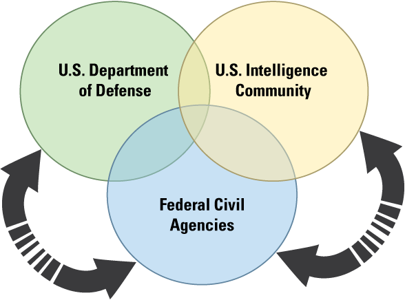
Diagram of the “triple junction” that depicts the relationship among Federal civil agencies, such as the U.S. Geological Survey, the U.S. Department of Defense, and the U.S. Intelligence Community.
Since the time of the Greeks and Persians, at about 500 B.C.E., maps have been critical to planning military campaigns (Defense Mapping Agency [DMA], 1982). General George Washington employed maps during the Revolutionary War. As a teenager, Washington trained as a surveyor (fig. 2) and assisted in surveying the city of Alexandria, Virginia (Va.). In July 1749, at the age of 17, he was appointed surveyor of Culpeper County, Va. Later, while serving in the military, Washington “applied his surveying and cartographic skills to military maps” (Noble, 1981, p. 178–180). Washington, in a message to John Hancock on January 26, 1777, stated that he was “obliged to make shift, with such Sketches as I could trace out from my own Observations, and that of Gentlemen around me” (Washington, 1998). Congress responded to Washington in 1777, authorizing him to establish a military cartographic headquarters that could supply maps for the U.S. Army’s military campaigns. This first U.S. Government-established mapping organization included a mix of military and civilian personnel (DMA, 1982). The knowledge Washington gained as a civilian surveyor is an early example of civil government training and experience benefitting the military (fig. 3).

An Ink sketch of young George Washington surveying the area around the Popes Creek, Virginia, plantation. Image appears courtesy of the National Park Service.
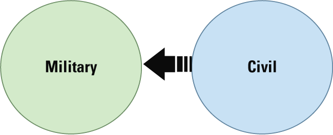
Diagram showing the relationship where the flow of knowledge goes from the civil government to the military.
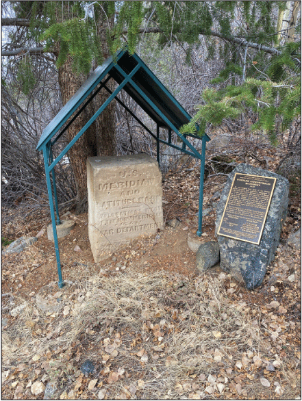
After the Revolutionary War, Congress appointed Thomas Hutchins as the Geographer of the United States, where he played a leading role in surveying and mapping the new Nation. Before the war, Hutchins was a British Army officer who mapped parts of present-day Ohio and Michigan and areas of the southern Colonies. He switched sides, joined the Continental Army, and supported the military campaigns in the South (DMA, 1982). Congress tasked Hutchins with starting the first public land survey, which was authorized by the passage of the Land Ordinance of 1785. That survey, now known as the Seven Ranges of Ohio (fig. 4), began on the northern shore of the Ohio River where it intersects with the present boundary of the States of Ohio and Pennsylvania. The first line surveyed, known as the Geographer’s Line, started at that point and ended 42 miles (mi) directly west. Townships 6-mi square were surveyed south of the Geographer’s Line to the Ohio River. The Seven Ranges was the first area surveyed under the U.S. Public Land Survey System (Noble, 1981, p. 184–189). Hutchins brought military training and experience to bear in the civilian government and contributed to surveying and mapping the country. To that end, figure 5 depicts the evolution of the collaboration model to show the flow of experience and knowledge from military to civilian sectors.
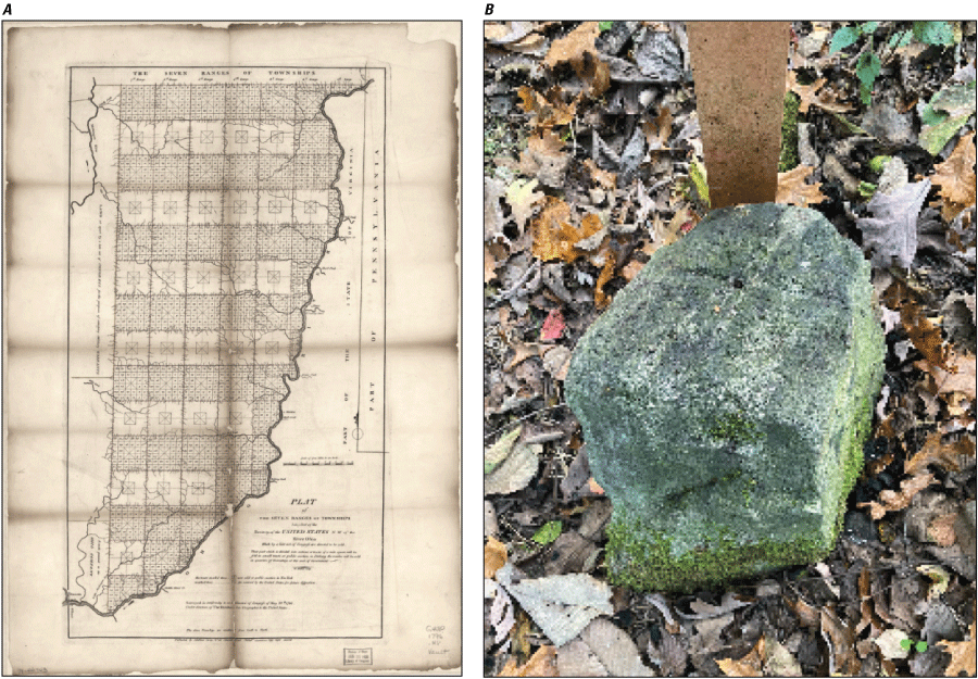
Two images, one of which (A) is a plat showing the Seven Ranges (Hutchins, 1796). The other (B) is a photograph of a stone that marks the western end of the Geographer’s Line and appears courtesy of Paul M. Young, U.S. Geological Survey.
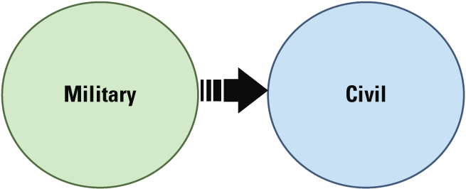
Diagram showing a relationship where the flow of knowledge goes from the military to the civil government.
Many explorers who traveled west of the Mississippi River in the time between the Nation’s independence and the Civil War were military men or those who previously served in the military, such as Meriwether Lewis, William Clark, John Fremont, Gouverneur Warren, William Emory, and Zebulon Pike, among others (Andregg, 1979). Their military training and experience enabled successful explorations and serve as another example of military service contributing to a civilian mission (fig. 5).
The U.S. Geological Survey (USGS) traces its military collaborations to John Wesley Powell (fig. 6), 10 years before the 1879 establishment of the USGS. In 1869, Powell, then a geology professor, drew U.S. Army rations at no cost for his journey and exploration of the Grand Canyon (Worster, 2001, p. 127, 131–132). This circumstance, too, is an example of the military aiding a civilian operation, as represented by figure 5. Powell became the second USGS Director in 1881.
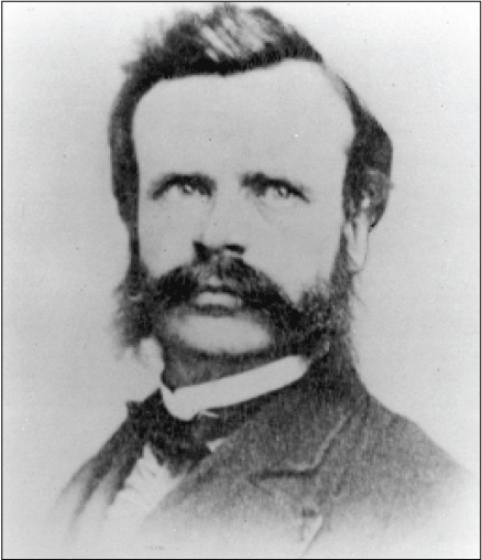
Photograph of John Wesley Powell taken in Chicago, Illinois,1869. Image appears courtesy of the U.S. Geological Survey Denver Library Photographic Collection.
At nearly the same time as Powell, U.S. Army Lieutenant George Wheeler began an extensive mapping effort of the American West, employing both military soldiers and civilian scientists, many of whom transitioned to the USGS at its establishment in 1879 (Andregg, 1979; U.S. Army Corps of Engineers [USACE], 2021). When completed, Wheeler’s maps satisfied civil and military needs and were the result of a close, collaborative relationship among the civil and military sectors. The diagram in figure 7 highlights the collaborative overlap between these two sectors.
The collaborative relationship is fluid, so that in times of national emergency, such as war, the civil sector’s people and resources can be brought to bear to support the military’s war efforts. During World War I, USGS topographic engineers—now known as cartographers—joined the military, where significant advances in map compilation were made from aerial photographs; after the war, civilian government mapping agencies, including the USGS, adopted these practices. The USGS provided vital mapping and geologic support to the military in its World War I and World War II efforts. This form of the cooperative relationship shows an almost complete overlap of the military and civilian sectors (fig. 8).
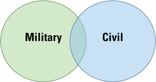
Diagram showing how military and civil government collaborate and work closely together to achieve joint missions.
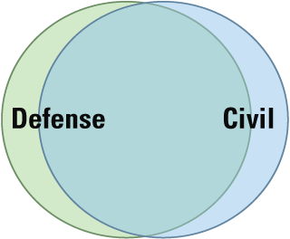
Diagram showing that in times of national emergency, as in World Wars I and II, nearly the full mapping capacity of the U.S. Geological Survey was brought to bear on the war efforts.
Shortly after World War II, the U.S. Army, using rockets developed by Germany, acquired the first image of the Earth taken from space. Beginning in the 1960s, the USGS gained access to Earth observation imagery from airborne and space-based military and IC classified sensors.
In the late 1960s, the USGS started updating its topographic maps with images acquired from classified satellites. Today, the USGS detects, assesses, and mitigates natural hazards, monitors environmental conditions, and studies land-surface changes with these data (Opstal and Rogers, 2022; Young, 2023). The early history described in this report laid the groundwork for the Earth mapping and observation collaboration that continues today.
This discussion leads to the relationship shown in figure 1. Congress formed the DOD from the merger of the then War and Navy Departments and established the Department of the Air Force and the Central Intelligence Agency by passing the National Security Act of 1947 (Public Law 80–253, 61 Stat. 495) on July 26, 1947. The Intelligence Organization Act of 1992 (Title VII of Public Law 102–496, H.R. 5095, 106 Stat. 3188) formally established the IC. Thus, the model (fig. 1) replaces the military with the DOD, representing the uniform military and civilian components, and incorporates the IC.
This report describes the USGS relationship—one of the Federal civil agencies represented in the “triple junction” model (fig. 1)—and its evolution. In the first 100 years of the USGS, from 1879 to 1979, collaboration with the military, and later the IC, involved sharing data, advances in technological development, and personnel (and their associated training). The intersection of a civil government, initially with the military and later with the IC, can be traced back to the origins of the Nation, as demonstrated by Washington and Hutchins.
Today, an example of the everyday use of military technology by the civil sector is the Global Positioning System (GPS). The GPS is a constellation of satellites (fig. 9) operated by the U.S. Space Force (USSF) that provides position, navigation, and timing data to military and civilian users (USSF, 2017). Wide-ranging areas of GPS civil applications include agriculture, aviation, environment, marine, public safety and disaster relief, rail, recreation, roads and highways, space, surveying and mapping, and timing (National Coordination Office for Space-Based Positioning, Navigation, and Timing, 2023). Location services are common applications found on many mobile devices with coordinates often originating or derived from GPS satellites.
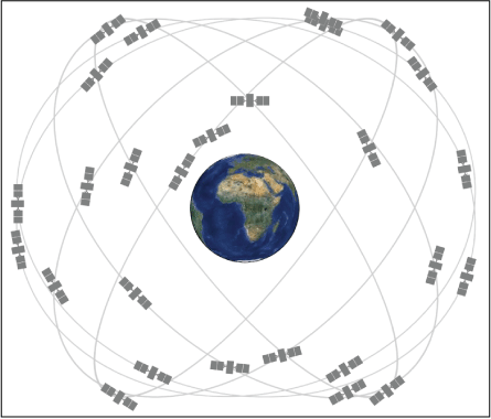
Data illustration showing a visual representation of the Global Positioning System satellite constellation around the Earth. Image appears courtesy of the Los Alamos National Laboratory.
The USGS, military, and IC collaboration is an example of “good government,” where different Federal agencies share data, technology development, and expertise in a way that allows the government to avoid redundant costs that might otherwise result from multiple agencies funding the same effort. Opstal (2017) coined the term “sunk cost well spent” to describe the Federal civil government’s use of military and intelligence remote-sensing data. This report traces the first 100 years of USGS collaboration with the military and IC in the mapping and Earth-observation sciences and provides examples of where the collaboration benefited one or more collaborators.
Early Collaboration
From the Nation’s founding until the establishment of the USGS in 1879, mapping the western frontier was the responsibility of the U.S. Army. More than 100 exploring and mapping expeditions were sent west between the Louisiana Purchase in 1803 and the Civil War (Evans and Frye, 2009, p. 1).
The USGS can trace its collaboration with the military to its second Director, John Wesley Powell, who received support from the Army in his explorations of the American West. After serving as a Union officer during the Civil War, Powell (fig. 6) became a science professor at Illinois Wesleyan University and later a professor in geology at Illinois State Normal University and curator of the University’s Natural History Museum. In 1867, he led a group of family, friends, and students on a natural science expedition to the Rocky Mountains of Colorado. Powell sought funding for the expedition from his former commander, General Ulysses S. Grant, who at the time was Chief of the Army. While Grant did not provide Powell with funds, he did authorize Powell to buy supplies from the Army at low government rates and offered a military escort, which Powell later declined (Worster, 2001, p. 114–117). Grant allowing Powell to draw Army rations at low cost is an early example of the military aiding a civilian mapping and science activity (fig. 5).
The 1867 trip inspired Powell to plan a more extensive exploration of the Colorado River through the Grand Canyon. Determining that an expedition would take a larger party and span more than a year, Powell sought funds to be spared the cost of buying food at frontier prices or even at the lower Army cost. In April 1868, he again approached Grant, who endorsed the expedition but still needed Congressional authorization to allow Powell to draw Army rations at no cost. Congress gave Grant the authorization (Worster, 2001, p. 127, 131–132). Powell and his party explored western Colorado into Utah from July to November 1868 (Worster, 2001, p. 136–153). In early 1869, he began to plan an expedition on the Green and Colorado Rivers through the Grand Canyon. His Congressional authorization to draw Army rations at no cost was still in effect (Worster, 2001, p. 57). Powell completed the trip through the Grand Canyon in August 1869 (fig. 10), a feat not known to have been done before (Rabbitt, 1989, p. 7). The Congressional authorization that provided Powell with Army rations at no cost is another case of military support for a civilian mission (fig. 5).
Powell was not the only person exploring the West. From 1867 to 1879, what came to be collectively known as the “Four Great Surveys of the West” were undertaken to locate resources needed by the country’s growing populations and industries. In 1867, Congress authorized a 25-year-old Yale University graduate, Clarence King, to form and lead the Geological Exploration of the Fortieth Parallel, also referred to as the King Survey, to look for natural resources along the recently completed transcontinental railroad route. In the same year, Ferdinand V. Hayden, M.D., assumed responsibility for the Survey of Nebraska, later expanded by Congress to the Geological and Geographical Survey of the Territories. After his successful trip through the Grand Canyon, Congress established the United States Geographical and Geological Survey of the Rocky Mountain Region with Powell in command. Powell continued to explore the West (fig. 11) until 1881, when he was appointed and confirmed as the second Director of the USGS, where he served until 1894 (Rabbitt, 1989, p. 12). A U.S. Army officer, George Wheeler, commanded the fourth Survey.
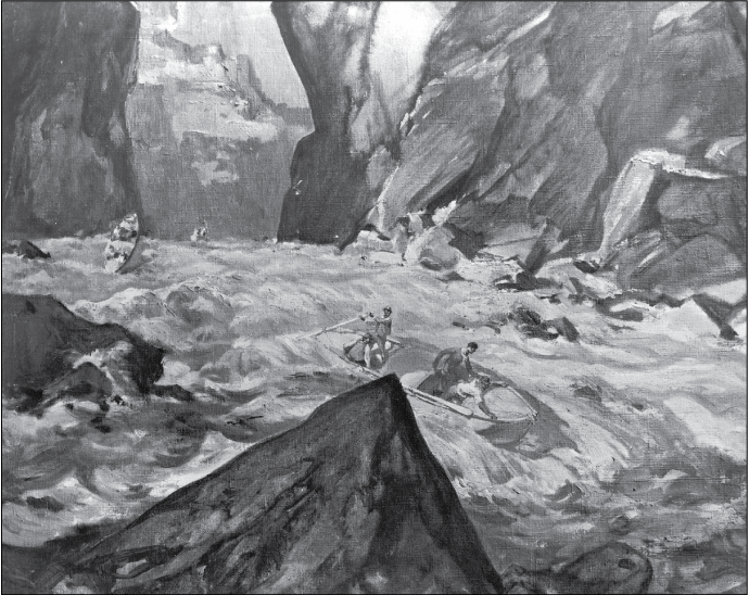
Painting of John Wesley Powell and his party in the Grand Canyon, presumably during the historic Colorado Expedition of 1869. Painting by Henry C. Pitz appears courtesy of the Smithsonian Institution, Bureau of American Ethnology, and the U.S. Geological Survey.
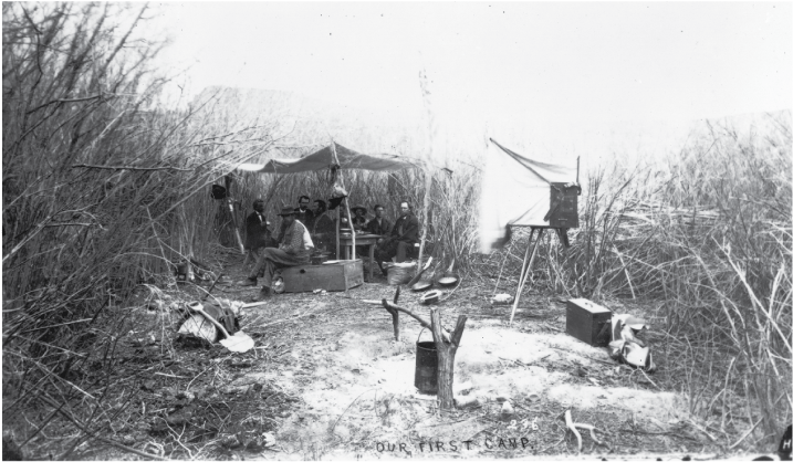
Photograph of the first camp of John Wesley Powell's second expedition. Shown from left to right are Professor Almon Harris Thompson, Andrew Hattan, S.V. Jones, John F. Steward, W.C. Powell, Frank C.A. Richardson, Frederick Dellenbaugh, and F.M. Bishop. Green River, Wyoming. May 4, 1871. Photograph by E.O. Beaman, U.S. Geological Survey (USGS), and appears courtesy of the USGS Denver Library Photographic Collection.
From 1869 to 1871, U.S. Army Lieutenant George Wheeler (fig. 12), an 1866 graduate of the U.S. Military Academy at West Point, New York, and a commissioned officer of the U.S. Army’s Corps of Engineers, mapped parts of Nevada and Arizona to support military missions. From July to November 1869, Wheeler and his party of 36 people, with 8 wagons, 48 mules, and 31 horses, conducted a military reconnaissance and mapped the area south and west of White Pine, Nevada (Rabbitt, 1979, p. 182–183). In 1871, Wheeler was ordered to explore and map eastern Nevada and Arizona to obtain information for military maps and collect data about the country’s physical features (Rabbitt, 1979, p. 196). Later, in 1871, based on his experiences, Wheeler proposed a plan to map the area west of the 100th meridian at a scale of 1 inch (in.) to 8 mi. The 100th meridian passes through central North Dakota, South Dakota, Nebraska, western Kansas, eastern Colorado, near the border between Oklahoma and the Texas Panhandle, and through Texas, near Abilene. He estimated a cost of $2.5 million and expected the work to take 15 years.
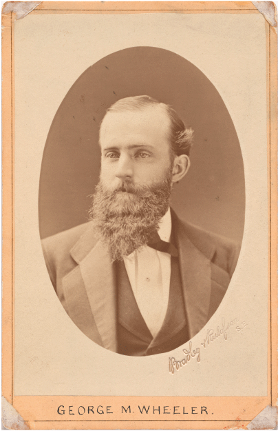
Photograph of U.S. Army Lieutenant George Wheeler, circa 1860–1869. Photograph appears courtesy of the National Portrait Gallery, Smithsonian Institution.
Wheeler planned to map the West by dividing the area into 95 rectangles along lines of latitude and longitude. Also referred to as quadrangles, those on the Pacific Ocean coast and the border with Mexico were partial rectangles based on the variability of the coast and the international border (fig. 13). According to Wilson (2010, p. 3), “This quadrangle concept was a precursor of the topographic and geologic mapping of quadrangles that the U.S. Geological Survey later adopted and still utilizes.” In 1872, Congress authorized the Geological and Geographical Survey of the Territories West of the 100th Meridian (fig. 14) and placed Wheeler in command (Rabbitt, 1979, p. 200). Between 1871 and 1879, Wheeler and his field parties mapped nearly one-fourth of the region west of the 100th meridian (Schubert, 1980, p. 149) in what is known as the Wheeler Survey. Wheeler hired military soldiers and civilian scientists skilled in astronomy, botany, chemistry, ethnology, geology, paleontology, and zoology. He supplemented his Army engineers with civilian topographers and surveyors (USACE, 2021).
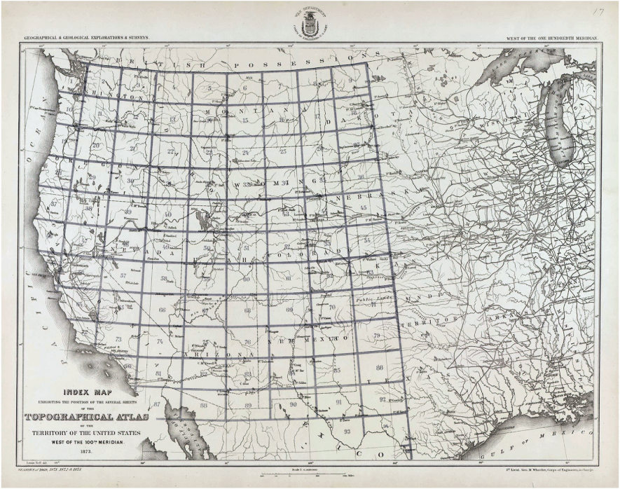
The Wheeler Survey index map (U.S. Geographical Surveys West of the 100th Meridian, 1889e).
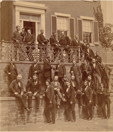
Photograph of Wheeler Survey members circa 1874. Standing in the top row, sixth from the left, is George M. Wheeler. Image appears courtesy of the National Portrait Gallery, Smithsonian Institution.
Figure 15 depicts the progress the Wheeler Survey had made by 1876. Haggit (2021a) tallied 89 map sheets published by the Wheeler Survey: 50 topographic maps (fig. 16), 11 geologic maps (fig. 17), and 28 land-classification maps (fig. 18) at scales of 1 in. to 8 mi (1:253,440), 1 in. to 4 mi (1:506,880), and 1 in. to 2 mi (1:126,720). The land-classification maps indicated areas suitable for agriculture, timber, and grazing or that were arid-barren. In some publications these were referred to as economic features (Haggit, 2021b).
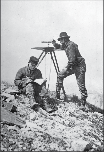
While Wheeler’s early mapping efforts were criticized as inaccurate, Powell praised the Wheeler Survey’s astronomical work (fig. 19), which provided the foundation for topographic mapping at that time (Wilson, 2010, p. 28). The King Survey also mapped areas of the west along the 40th line of latitude, generally following the transcontinental railroad (fig. 15). Wheeler’s plans to subdivide the country into rectangles along lines of latitude and longitude persist in today’s USGS topographic and geologic mapping programs.
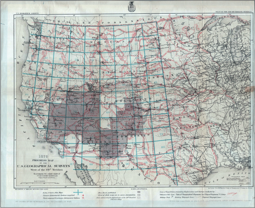
Wheeler Survey progress map (U.S. Geographical Surveys West of the 100th Meridian, 1889a). Shaded areas are map sheets published or in preparation. The lighter shading is the area mapped by the King Survey.

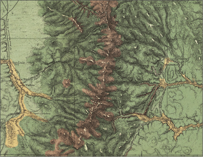
A portion of the Wheeler Survey topographic map—atlas sheet number 70 A, parts of southern Colorado and northern New Mexico—was originally published at 1 inch to 4 miles, 1:253,440 scale (U.S. Geographical Surveys West of the 100th Meridian, 1889b). Image appears courtesy of the David Rumsey Map Collection, David Rumsey Map Center, Stanford Libraries. Image is provided under an Attribution-NonCommercial-ShareAlike 3.0 Unported (CC BY–NC–SA 3.0) license (https://creativecommons.org/licenses/by-nc-sa/3.0/).
On March 3, 1879, Congress established the U.S. Geological Survey, merging the Powell, King, Hayden, and Wheeler Surveys. King became the first USGS Director, while Hayden continued his explorations as a USGS employee. Powell remained in the West to complete his work and became the second USGS Director in 1881 following King’s resignation. With the establishment of the USGS, Wheeler’s survey work transitioned into the new organization, effectively changing the mapping of the West from a military mission to a civilian responsibility. According to Andregg (1979), many of the topographers from the Wheeler and Powell surveys joined the newly established USGS. However, Wheeler remained an Army officer and continued his military career. As USGS Director, one of Powell’s priorities was topographic mapping, which built upon the work of Wheeler and the other “Great Surveys of the West” in mapping the Nation (Rabbitt, 1980, p. 9). Congress authorized the systematic topographic mapping of the United States after Powell’s testimony in 1884 (Usery and others, 2010, p. 5).
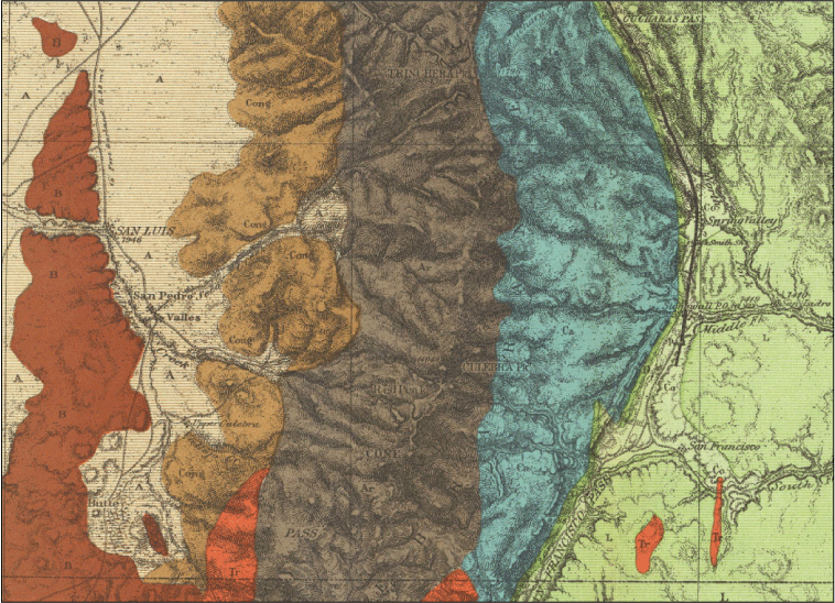
A part of the Wheeler Survey geologic map, atlas sheet number 70 A, parts of southern Colorado and northern New Mexico, originally published at 1 inch to 4 miles, 1:253,440 scale (U.S. Geographical Surveys West of the 100th Meridian, 1889d). Image appears courtesy of the David Rumsey Map Collection, David Rumsey Map Center, Stanford Libraries. Image is provided under an Attribution-NonCommercial-ShareAlike 3.0 Unported (CC BY–NC–SA 3.0) license (https://creativecommons.org/licenses/by-nc-sa/3.0/).
A part of the Wheeler Survey economic features map, atlas sheet number 70 A, parts of southern Colorado and northern New Mexico, originally published at 1 inch to 4 miles, 1:253,440 scale (U.S. Geographical Surveys West of the 100th Meridian, 1889c). Economic features maps depict areas with potential for agriculture, timber, and grazing, and arid or barren areas. Image appears courtesy of the David Rumsey Map Collection, David Rumsey Map Center, Stanford Libraries. Image is provided under an Attribution-NonCommercial-ShareAlike 3.0 Unported (CC BY–NC–SA 3.0) license (https://creativecommons.org/licenses/by-nc-sa/3.0/).
Before becoming USGS Director, Powell turned to the Army to support his civilian scientific and mapping efforts, and he received support from both General Grant and Congress. Wheeler’s plan to divide the country into quadrangles for mapping purposes remained with the USGS. Initially, the USGS mapped the country at a scale of 1:250,000, where 1 in. on the map represents approximately 4 mi on the ground and covers 1 degree of latitude by 1 degree of longitude and 1:125,000-scale for 30-minute maps, where 1 in. on the map is approximately 2 mi on the ground. Over time, the USGS mapped in greater detail until the 1950s, when the standard mapping scale became 1:24,000, and each map covered 7.5 minutes of latitude by 7.5 minutes of longitude and 1 in. on the map represents 2,000 feet (ft) on the ground (Thompson, 1987, p. 6, 20). Today’s USGS topographic map product is modeled on the historical 1:24,000-scale topographic maps (Davis and others, 2018, p. 1). Powell and Wheeler also set the stage for subsequent USGS-military collaboration in the mapping sciences.
Photograph of the Wheeler Survey astronomical monument above Georgetown, Colorado. Historical markers and protective covers were placed in 2007 (Wilson, 2010). Photograph taken November 2023 and appears courtesy of Paul M. Young, U.S. Geological Survey.
War Induces Collaboration
World War I saw advances made in the use of aerial photography for military purposes and USGS employees supported these efforts. A large percentage of USGS resources went to supporting the war efforts, which led to a relationship that shifted from being a civil-government experience that benefited the military (fig. 3) to a close, collaborative relationship (fig. 8).
By the early 1900s, the USGS map makers had used telescopic alidades and plane tables (fig. 20) to measure vertical angles, calculate point positions, and determine the elevations necessary for compiling a topographic map. An alidade is a precision telescope used to measure angles and distances and a plane table helps the measurements be translated into a map (Evans and Frye, 2009, p. 146).
Photograph illustrating the use of a plane table and telescopic alidade, Canadian boundary, circa 1906. Photograph appears courtesy of U.S. Geological Survey Denver Library Photographic Collection.
World War I saw the introduction of aerial photographs into the process of map compilation. The war started in 1914; the United States entered the war in April 1917. In this interim period, the USGS increased its efforts to support the military’s war preparations. In response to a War Department request, the USGS established a Division of Military Surveys within the Topographic Branch and received $35,000 from the War Department for mapping (Rabbitt, 1986, p. 176). The Army commissioned USGS topographic engineer Glenn S. Smith, a USGS employee since 1886, and put him in charge of the new division (Evans and Frye, 2009, p. 77). In March 1917, as war seemed inevitable, the Topographic Branch suspended its domestic fieldwork and redirected all available funds into making maps for the War Department (Rabbitt, 1986, p. 177; Evans and Frye, 2009, p. 77). As Rabbitt (1989, p. 27) stated about personnel use after the United States entered the war, “The majority of the technical personnel of the Topographic Branch were commissioned in the Army's [sic] Corps of Engineers.” Evans and Frye (2009, p. 81–82) report that 479 USGS employees served in the military during the War (fig. 21), the majority of whom (305 people) were from the Topographic Branch and represented nearly 100 percent of its staff. This military service brought mapping expertise to the Army and the Nation’s war efforts (Campbell, 2008, p. 90; Evans and Frye, 2009, p. 77).
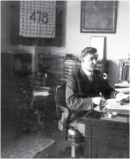
Photograph of George Otis Smith, director of the U.S. Geological Survey (USGS) from 1907 to 1930; photograph taken circa. 1918. The flag in the background refers to members of the USGS serving in the military (478 servicemen) during World War I. This number differs by one from that of Evans and Frye (2009, p. 81–82). Photograph credit is the USGS, and the photograph appears courtesy of the USGS Denver Library Photographic Collection.
The idea of using aerial photographs for military observations in making maps was not new when World War I started. French photographer Gaspard-Félix Tournachon, known as Nadar, is credited with the idea of taking aerial photographs of military operations from a balloon. Nadar offered his services to the French Army in 1859 to support their operations in Italy. It is not known if they accepted. Aerial photography from balloons was considered in the Civil War (1861–1865) and the 1870–1871 Franco-Prussian War. However, due to the bulky photography equipment and long exposure times required by the technology, it was impractical to take a photograph from a balloon (Haydon, 2000, p. 330–334). In 1908, a photographer accompanied Wilbur Wright on a flight over Le Mans, France, and took the first aerial photograph from an airplane. Capturing aerial photographs from airplanes (fig. 22) has advantages over a balloon. Airplane flights can be directed, including over hostile territory; kites and balloons, however, must be tethered in areas controlled by friendly forces or allowed to float free but uncontrolled (Lillesand and others, 2015, p. 88).
World War I saw significant developments in aerial photography, and USGS employees supported these developments. James W. Bagley (fig. 23), a USGS topographic engineer, was an early adopter of using photography to make maps. In the years before World War I, he led a USGS team that used a panoramic-film camera to map interior parts of Alaska. Panoramic photography is taken at the ground level of the landscape or from natural vantage points such as hills or mountains to gain a better perspective. Measurements necessary to compile a topographic map would then be taken using a photographic alidade. Photography was necessary to map Alaska’s large, unmapped areas in the short, northern-latitude field seasons.
Photography was collected during the summer and later measured in the USGS office in Washington, D.C., during the off-season (Collier, 2002; Schneider, 2017). Bagley looked ahead to the use of aerial cameras on airplanes. In 1917, he wrote, “In view of the increasing importance of photography in surveying and the rapid strides that are being made in the art of navigating air craft [sic] it has seemed desirable to include also some notes on the application of photogrammetry to aerial surveys” (Bagley, 1917, p. 9). The last chapter of his landmark 1917 publication is devoted to aerial photography, in which he foresaw the use of aerial photographs for military reconnaissance (Bagley, 1917, p. 64). As Schneider (2017) notes: “His expertise as a topographic engineer, plus his research into aerial photography for mapping would be invaluable in determining enemy locations and battle lines.” Bagley went on to serve in the U.S. Army during the war where he, along with Fred H. Moffit and John B. Merte, designed and constructed aerial cameras (Rabbitt, 1986, p. 187). When the war ended in 1918, Bagley was working on an experimental three-lens aerial camera (Campbell, 2008, p. 86), which Collier (2002) calls the most significant development in civilian photogrammetry. Bagley remained in the Army until 1936, continuing to make advancements in aerial photographic surveys (Schneider, 2017).
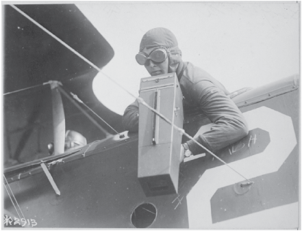
Photograph of Aeroplane Graflex camera in action, circa 1917–1918. Photograph credit: U.S. Department of Defense. Image appears courtesy of the National Archives and Records Administration.
Photograph of Major James Warren Bagley, topographic engineer and commander of the 29th Engineer Regiment. Photograph appears courtesy of the U.S. Army.
Another notable USGS employee who joined the war effort was Glenn S. Smith (fig. 24). In January 1917, Smith was put in charge of the Division of Military Surveys and served as the assistant to the U.S. Army’s Chief of the Topographical Division in France (Evans and Frye, 2009, p. 77). Commissioned as a major, the Army later promoted Smith to lieutenant colonel (Rabbitt, 1986, p. 184). In France, Smith was responsible for printing, and from July 1 to November 11, 1918, he oversaw the printing of over 5 million maps (Campbell, 2008, p. 91).
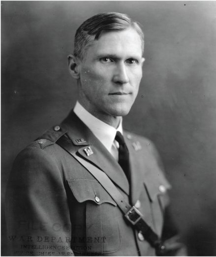
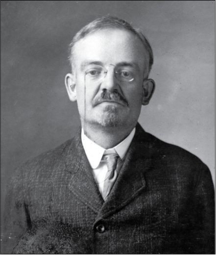
Claude H. Birdseye (fig. 25) was another enlistee. When the war started, Birdseye already had 13 years of service with the USGS and was the topographic engineer of the Rocky Mountain Division. Commissioned as an Engineer Officers Reserve Corps captain, he was promoted to major before leaving for France (Rabbitt, 1986, p. 185). Birdseye supervised other USGS employees who were instructors in the U.S. Army’s Artillery School and oversaw the Army’s ranging and map information (Evans and Frye, 2009, p. 78; Rabbitt, 1986, p. 196).
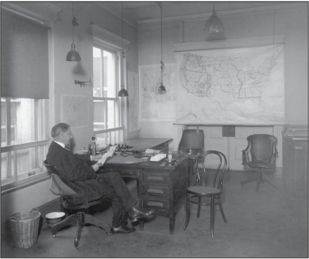
Photograph of Glenn S. Smith in his U.S. Geological Survey (USGS) office, Washington, D.C., 1917. Photograph appears courtesy of the USGS Denver Library Photographic Collection.
Photograph of Claude H. Birdseye, Chief Topographic Engineer, 1916. Photograph appears courtesy of the U.S. Geological Survey Denver Library Photographic Collection.
The American Expeditionary Forces (AEF) published a booklet in March 1918 to “put under one cover all information concerning maps which an officer not engaged in the actual topographical work will have occasion to use” (AEF, 1918). The booklet included a section on aerial photographic interpretation with examples taken from aerial photographs and mapped features to help officers identify cultivation and woodlands, infantry and artillery positions, military camps and depots, and communications features. This situation is likely the first time many officers had seen and used aerial photographs since before the war, as they were not commonly used in military operations. According to Campbell (2008, p. 77), “It is difficult to find an account of the history of remote sensing, or of the development of aerial photography, that does not cite World War I as a prominent landmark.” Campbell (2008, p. 92) also calls World War I the “incubator for the development of aerial photography and photointerpretation.” Cloud (2002) called aerial photography “one of the triumphant technologies of World War I.” The U.S. Army formed the 29th Engineers as the Army’s primary map-making organization, and many USGS topographic engineers were assigned to the organization (Campbell, 2008, p. 91). Over 1 million aerial photographs were taken during World War I (Lillesand and others, 2015, p. 88). Beyond making maps, aerial photography was also used “for pinpointing artillery fire and for reconnaissance of military material deployment and troop movements” (Werle, 2016).
The technology and experience using aerial photography would be in great demand in the United States after the war. Among developed nations, the United States was poorly mapped compared to European countries, and the newly developed science of photogrammetry would continue to be developed by those who gained experience in the war. Photogrammetry would be more cost-effective for topographic mapping than the traditional ground surveys most often used before the war (Collier, 2002).
The years following World War I saw former Army enlisted personnel and officers back working in their civilian government agencies, including the USGS, and founding aerial photography companies (Lillesand and others, 2015, p. 88). Smith, Birdseye, and many others brought their war-time mapping experiences back with them to their civilian jobs and made significant contributions to the mapping sciences and the development of aerial photography and photogrammetry in the making of topographic maps (Campbell, 2008, p. 86). Bagley, along with six other former USGS employees, remained in the Army after the war (Evans and Frye, 2009, p. 80). John H. Wilson, a lieutenant at the end of the war, remained in the Army and achieved the rank of brigadier general during World War II (Evans and Frye, 2009, p. 78).
Smith and Birdseye returned to the USGS, continuing their distinguished careers serving in various senior positions. After the war, Smith helped plan the mapping of the Island of Santo Domingo (Hispaniola) and was put in charge of mapping surveys in the West Indies and other Latin American countries (Rabbitt, 1986, p. 199). Birdseye returned to his position of Chief of the Rocky Mountain Division. In 1923, he led an expedition to compile a new map of a 251-mi stretch of the Grand Canyon (fig. 26) (Rabbitt 1986, p. 238). From 1929 to 1932, he led the mapping of the area where the Hoover Dam was built. Outside of the USGS, Birdseye was active in professional circles where he served as the first president of the American Society of Photogrammetry (now the American Society of Photogrammetry and Remote Sensing), president of the American Association of Geographers, and was active in the American Association for the Advancement of Science (Rabbitt 1986, p. 185).
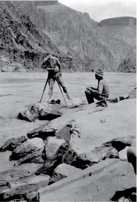
Photograph of Claude H. Birdseye and R.W. Burchard working in Upper Granite Gorge, Grand Canyon, 1923. Photograph appears courtesy of the U.S. Geological Survey Denver Library Photographic Collection.
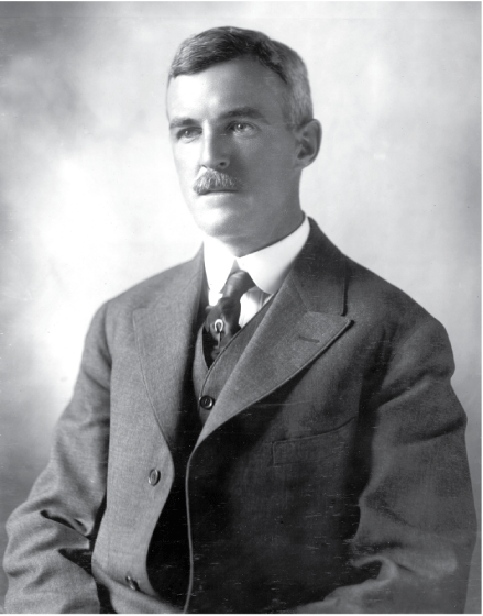
Topographic mapping expertise was not the only contribution the USGS made to the country’s World War I efforts. The Army commissioned USGS geologist Alfred H. Brooks (fig. 27) as a major—later, he became a lieutenant colonel. He served as the chief geologist of the AEF and was part of the first contingent to sail to France in June 1917. From 1902 to 1924, Brooks was the USGS chief Alaskan geologist. Following his 1924 death, in 1925 the U.S. Board on Geographic Names named the Brooks Range in northern Alaska for him (Rabbitt, 1986, p. 180–182). During the war, Brooks oversaw the compilation of geologic and water-supply maps (Rabbitt, 1986, p. 196). Information on soils and subsoils within 4 ft of the surface contributed to the construction of trenches, dugouts, and covered ways (Rabbitt, 1986, p. 183).
Photograph of Alfred H. Brooks, who served as the U.S. Geological Survey (USGS) chief Alaskan geologist from 1902 to 1924. Photograph appears courtesy of the USGS Denver Library Photographic Collection.
As another result of the war effort, the USGS received surplus Army trucks, which were then used to aid in field work (fig. 28). The military made significant technological advancements in mapping using aerial photographs during World War I. The USGS benefited from those advancements and applied them to its topographic mapping mission after the war. The investments in mapping technology made by the military allowed the USGS to avoid spending money unnecessarily. As war transitioned to peace, the collaborative relationship shifted as well, from one of almost total overlap (fig. 8) during the war to one of continued collaboration benefiting both governmental sectors (fig. 7).
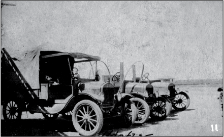
U.S. Geological Survey (USGS) trucks at Barnhart, Texas, received from the U.S. Army at Kelly Field, San Antonio, Texas, 1920. Photograph appears courtesy of the USGS Denver Library Photographic Collection.
Collaboration Between World Wars
The time between World Wars I and II saw tremendous development in photogrammetry. USGS topographic engineers and the military played a significant role in that development. The trained photogrammetrists who gained experience in the 1930s supported efforts in World War II due to the magnitude of the number of maps that had to be made (Collier, 2002).
According to Mack (1990, p. 32), “surplus military reconnaissance equipment, fed a small civilian, aerial photography industry which provided photographs used primarily for mapping in geological explorations.” However, those companies took time to develop, and government agencies, such as the USGS, continued to rely on military aircraft and pilots to meet their aerial mapping needs. This relationship was mutually beneficial (fig. 7). Military commanders sought peacetime work for planes and pilots. The U.S. Army Air Service performed aerial mapping to maintain proficiency and keep planes flying (Mack, 1990, p. 32).
In 1919, to foster the mapping relationships between the military and those personnel now returned to civilian status that had developed mapping skills during the war, Major General William M. Black, U.S. Army Chief of Engineers—taking advice from a board of nine officers he appointed—promoted the establishment of the Society of American Military Engineers (SAME) and the formation of the Society’s journal: The Military Engineer. The journal published the following statement in its January–February 1920 edition:
“We are establishing at this time a Society of American Military Engineers. This society will serve no selfish purpose. It is dedicated to patriotism and national security. Its objects are, in brief, to promote solidarity and co-operation between engineers in civil and military life, to disseminate technical knowledge bearing upon progress in the art of war and the application of engineering science thereto, and to preserve and maintain the best standards and traditions of the profession, all in the interests of patriotism and national security.” (SAME, 2022)
USGS employees played an active role in the new society. Eight USGS employees were SAME charter members and among the Society’s first officers. From 1920 to 1943, USGS employees contributed 30 articles on mapping topics to “The Military Engineer” (Evans and Frye, 2009, p. 88).
The USGS lost no time taking the mapping lessons learned during the war and applying them to its domestic mapping mission, and close collaboration with the military continued. Without airplanes of its own and private sector companies just beginning to form, the USGS relied on Army and Navy airplanes to fly and acquire aerial photographs. The USGS mapped the Schoolcraft, Michigan (Mich.), quadrangle using aerial photographs acquired by the U.S. Army Air Service in June 1920. The 1:62,500-scale (1 in. on the map is about 1 mi on the ground) quadrangle covering about 220 square miles (mi2) was flown in 7 hours. Roads, streams, and forests were mapped from the photographs (Rabbitt, 1986, p. 215). The final map was published in 1922 (fig. 29). The U.S. Army Air Service gained valuable experience taking aerial photographs to support the USGS in this project.
In 1926, the Navy flew aerial photographs in southeastern Alaska (fig. 30) using an Army camera designed by former USGS topographic engineer and then Army officer James Bagley. During one field campaign, the Navy photographed about 10,000 mi2 (Sargent and Moffit, 1929, p. 144–152). At the request of the USGS, the Navy collected about 20,000 mi2 of aerial photography between the two World Wars (FitzGerald, 1951, p. 1). The Navy also gained valuable experience flying aerial-photography from their support of the USGS. Further experiments and testing of how aerial photographs could be used for mapping were led by Thomas P. Pendleton, who served as a second lieutenant during the war (Rabbitt, 1986, p. 215). In 1928, the USGS issued new topographic instructions in six chapters, one of which covered using aerial photography and photogrammetry in compiling topographic maps (USGS, 1928).
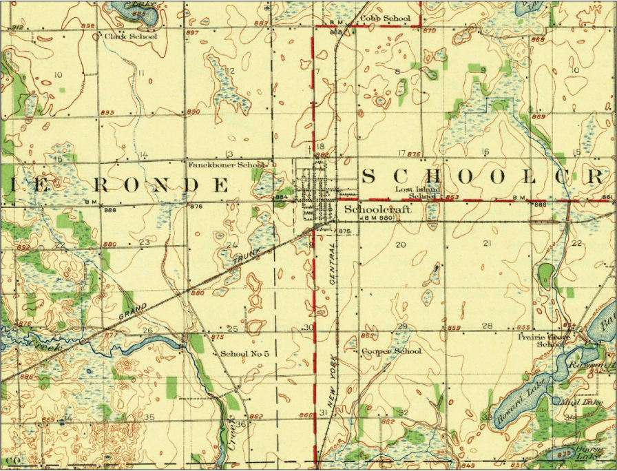
Section of a historical map showing part of the U.S. Geological Survey’s (USGS) Schoolcraft, Michigan, 1:62,500-scale quadrangle, the first USGS topographic map to be compiled, in part, from aerial photographs (USGS, 1922; Rabbitt, 1986, p. 215).
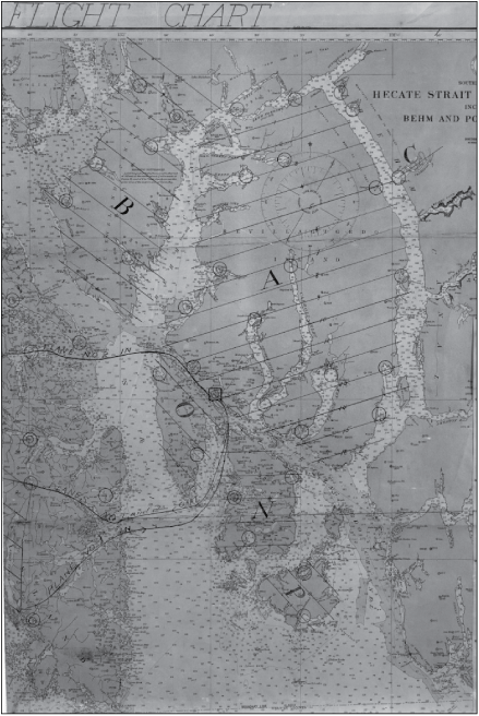
Photograph of the flight chart, Revillagigedo Island and vicinity, on a southeast Alaska flight map, 1926. Photograph by Rufus Harvey Sargent appears courtesy of the U.S. Geological Survey Denver Library Photographic Collection.
The USGS transitioned to using aerial photography and photogrammetry for topographic map compilation with its Tennessee Valley Mapping Program, which was initiated in 1934 using funds from the Public Works Administration. To meet its water control mission for the river basin, the Tennessee Valley Authority (TVA) quickly needed detailed maps for planning to cover the over 40,000 mi2 river basin, necessitating 766 maps at a scale of 1:24,000 (1 in. on the map equals 2,000 ft on the ground). Aerial photography and photogrammetric techniques had to be used to complete the task in the required time (Rabbitt, 1986, p. 350, 353–354; Evans and Frye, 2009, p. 102). To accomplish this mission, the USGS used overlapping aerial photographs that, when projected using a stereoplotter, showed the operator the terrain in three dimensions (fig. 31). With this method, contours (lines of equal elevation), roads, woodland, hydrography, and cultural features were mapped (Usery and others, 2010). The USGS–TVA project was led by World War I veteran Thomas P. Pendleton, who helped develop aerial cameras during and after the war and led the USGS Photographic Mapping Section (Rabbitt and Nelson, 2015, p. 47). The USGS–TVA mapping program made great strides in map compilation using newly developed photogrammetric equipment. They gained confidence after the U.S. Army Air Forces (USAAF), the year before, bought and tested the same equipment (Collier, 2002).
Building upon the military’s investments in airplanes, aerial cameras, and compiling maps from aerial photographs, the USGS transitioned to using aerial photography to create its topographic maps. As Cloud (2002) points out, “Before World War II, federal civilian and military mapping programs were supposedly distinct but complexly interrelated, particularly because many civilian agencies had inherited their programs from previous military efforts.” The time and expenses saved by the USGS in using the mapping investments made by the military are incalculable. This collaborative relationship persisted and benefited both parties (fig. 7).
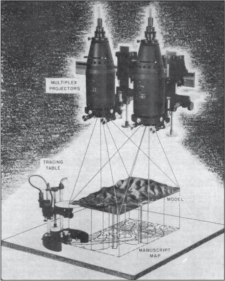
Image that shows a general overview of the multiplex mapping process. The image displays the coordinated use of multiplex projectors, a tracing table, and a model to create a manuscript map (Loud, 1952, pg. 7).
War Inspires Cooperation
As in World War I, the USGS provided mapping expertise to the military during World War II. Following the 1939 start of the war in Europe, collaboration increased between the USGS and the War Department, eventually turning into a close relationship (fig. 8).
Before the war, the USGS Alaska Branch was compiling detailed maps in southeastern and south-central Alaska for prospective airfields, reconnaissance maps to aid aerial navigation, and hydrographic charts for the Navy (FitzGerald, 1951, p. 14, 19). In 1940, the U.S. Army Engineers provided $1.210 million to the USGS to support strategic mapping, most of which were coastal areas (Rabbitt and Nelson, 2015, p. 33). Because of the USGS’s role in strategic mapping, mineral investigations, and water-supply studies in support of the War Department, Congress designated the USGS a defense agency in 1941 (Rabbitt and Nelson, 2015, p. 42–43). In appropriating money to the USGS in 1941, Congress provided $1.962 million, stipulating that not less than half be spent to map areas designated by the Secretary of War (Rabbitt and Nelson, 2015, p. 43–44).
During the war, Congress appropriated money for strategic mapping to the War Department, which then transferred the money to the USGS (Rabbitt and Nelson, 2015, p. 63). The initial focus on mapping coastal areas diminished after the threat of a Japanese invasion decreased, and the USGS turned its attention to producing maps of foreign areas under the War Department’s direction (Rabbitt and Nelson, 2015, p. 75).
By June 1943, nearly 67 percent of the 241 quadrangles published and 88 percent of the 684 maps in progress were designated by the War Department (Rabbitt and Nelson, 2015, p. 76). For the fiscal year ending June 30, 1945, the War Department transferred $1.060 million to the USGS to strategically map war zones (Rabbitt and Nelson, 2015, p. 117). During the war, the USGS mapped about 80,000 mi2 of war zones (Evans and Frye, 2009, p. 108).
Evans and Frye listed five ways the USGS Topographic Branch supported the war effort from 1941 to 1945:
-
1. “Conducted the necessary field surveys of areas in the strategic war zone of the United States as defined by the War Department, and prepared the resulting topographic maps for reproduction.
-
2. Compiled and prepared aeronautical approach charts of the continental United States, and target charts of Yugoslavia for the Army Air Forces.
-
3. Revised from aerial photographs the data on existing local topographic maps of Holland, France, and Italy, and redrafted the revised maps according to specifications for the Army Map Service.
-
4. By stereophotogrammetric methods, compiled topographic maps from aerial photographs for the Army Map Service of areas in France, Italy, Yugoslavia, Luzon, and the Sulu Archipelago of the Philippines, Austria, Belgium, China, Formosa [Taiwan], Ryukyu [sic] Rhetta [Japan’s Ryukyu Islands], and Japanese City Plains.
-
5. Prepared relief shaded maps of Japan, China, Manchuria, Korea, Formosa, Hainan, and South Central Europe for the U.S. Army Air Forces, and the General Staff, War Department” (Evans and Frye, 2009, p. 107–108).
In addition to producing maps for the military, the USGS trained military personnel, officers, and civilians from foreign countries (Evans and Frye, 2009, p. 108). During the war, 189 members of the USGS Topographic Branch entered the military; the total number of branch personnel during the war ranged from 485 to 745. Topographic Engineers remaining with the USGS were actively compiling maps in support of the War Department (Evans and Frye, 2009, p. 107–108).
Several USGS employees played key mapping roles while serving in the military. One such individual was Daniel Kennedy, who served in both World Wars. Kennedy enlisted in the Missouri National Guard in 1917 at age 17 and served in France, where he was wounded twice in battle and sent back to the United States. His recovery took 2 years. While in training, he met Captain Harry Truman, whom he later reconnected with during World War II when Truman was a U.S. Senator (Kennedy, 1998, p. 7–31). In 1926, Kennedy graduated from the Missouri School of Mines with a degree in civil engineering and, in 1935, earned the equivalent of a master’s degree (Kennedy, 1998, p. 34). In 1926, he started working for the USGS as a junior engineer (Kennedy, 1998, p. 38).
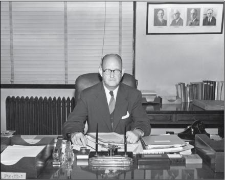
In 1942, Kennedy entered the U.S. Army Corps of Engineers (USACE) as a captain, was later promoted to major and then lieutenant colonel, and by 1944 was serving as General George S. Patton, Jr.’s chief mapmaker as Patton led the Third Army through France and into Germany. In one case, Kennedy oversaw the coordinate conversion and translation of a 1:250,000-scale German map to facilitate Patton’s move across France. About 150,000 copies of the map were printed. At one point during the war, a German artillery unit appeared to target a house where Patton was staying. Kennedy helped locate the artillery unit by converting a German coordinate system to the American system, which allowed the Army to locate and destroy the artillery. For Kennedy’s efforts, Patton himself pinned a Bronze Star on him (Kennedy, 1998, p. 56–80). By 1948, Kennedy (fig. 32) was back at the USGS and serving as the Central region engineer in Rolla, Missouri (Mo.) (Rabbitt and Nelson, 2015, p. 264). The Central region was at that time responsible for mapping the States of North Dakota, South Dakota, Minnesota, Wisconsin, Michigan, Nebraska, Iowa, Illinois, Kansas, Missouri, Oklahoma, Arkansas, Texas, and Louisiana (Evans and Frye, 2009, p. 123). In 2001, the USGS helped Kennedy celebrate his 100th birthday by presenting him with a letter from USGS Director Charles Groat (Beydler, undated).
Photograph of Daniel Kennedy, Central region engineer, 1952; appears courtesy of the U.S. Geological Survey Denver Library Photographic Collection.
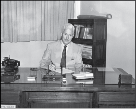
Another notable USGS employee who joined the military was Gerald Arthur FitzGerald, who joined the USGS in 1917 and worked on revising Alaskan aeronautical charts. According to Evans and Frye (2009, p. 64), the USGS Alaskan Branch, with FitzGerald as senior topographic engineer, “became the school for the Aeronautical Chart Service.” In 1942, the USAAF commissioned FitzGerald as a major (and later colonel), and he led the Aeronautical Chart Service. The American Society of Photogrammetry awarded FitzGerald its first Fairchild Award in 1944. General Henry “Hap” Arnold wrote the presentation in which he recognized FitzGerald, then an Army lieutenant colonel, for his contributions to aeronautical chart production (Arnold, 1944). In his acceptance address, FitzGerald recognized the contributions made by the USAAF and the USGS (FitzGerald, 1944). After the war, he returned to the USGS (fig. 33), and, in 1947, was appointed chief topographic engineer (Rabbitt and Nelson, 2015, p. 212). In 1951, he published the USGS history of Alaskan surveying and mapping as it had been done to date (FitzGerald, 1951).
Photograph of Gerald FitzGerald, chief topographic engineer, 1952; appears courtesy of the U.S. Geological Survey Denver Library Photographic Collection.
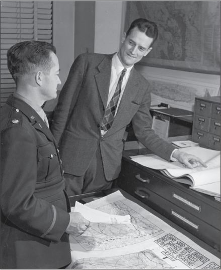
Photograph of Major Arthur R. Spillers, assistant, Military Intelligence Division, Office of the Chief Engineer (left), and Charles B. Hunt, Geologist in Charge, Military Geology Unit, U.S. Geological Survey (USGS) (right), talking over an assignment, circa 1940’s. Photograph appears courtesy of the USGS Denver Library Photographic Collection.
As in World War I, the USGS contributed more than topographic maps to the military. In 1942, the USGS established the Military Geology Unit (MGU) to do terrain analysis, create maps, and engage in other geologic studies (Rabbitt and Nelson, 2015, p. 63). Rather than transfer civilian geologists to the military, USGS geologists stayed with the USGS and contributed reports and geologic maps from their home offices (fig. 34). Throughout the war, the USGS contributed 88 geologists, 11 soil scientists, 15 other professionals, and 43 support staff to the MGU, who produced “140 major terrain folios, 42 other major reports, and 131 minor studies, overall containing about 5,000 maps [fig. 35], 4,000 photographs and figures, 2,500 large tables of data, and 140 terrain diagrams” Nelson and Rose (2012). One example of the USGS’s expertise in the war effort was identifying where Japanese balloon bombs were being manufactured and launched. In 1944 and 1945, Japan released over 9,000 balloons bombs, hoping they would reach the United States. The military asked the USGS to identify the sand from the balloon ballasts. Julia Garnder, Kathryn Lohman, and Kenneth Lohman narrowed the source of the sand to two beaches. The military bombed nearby factories making the balloons (Rabbitt and Nelson, 2015). Lists of the reports and maps of the MGU can be found in Leith and Bonham (1997).
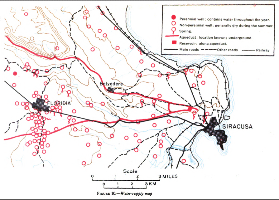
Water-supply map that is an example of maps produced by the U.S. Geological Survey (USGS) Military Geology Unit during World War II. Map originally appeared as figure 10 in USGS (1945).
The USGS continued to support the military’s mapping needs after World War II. The military relied on the USGS to produce aeronautical charts for Alaska, where the USAF flew aerial photography missions necessary for the USGS to map the principal transportation routes into Alaska’s interior (FitzGerald, 1951, p. 1). The USGS compiled a large-scale map of Naval Oil Shale Reserves Nos. 1 and 3 in Colorado for the Navy Department (Rabbitt and Nelson, 2015, p. 212). In 1952, the USGS Topographic Division established the Special Mapping Branch to continue aeronautical chart compilation to support the USAF (Evans and Frye, 2009, p. 135–137). In addition, the USGS mapped Bikini Atoll in support of Operation Crossroads, the testing of atomic bombs in 1946 (Rabbitt and Nelson, 2015, p. 212–214). In support of mapping needs in Alaska, the USAF and Navy acquired about 59,000 mi2 of aerial photography. The USGS and the military long coordinated on Alaskan mapping projects (Rabbitt and Nelson, 2015, p. 266). Evans and Frye reported in 1952 that “more than 50 percent of the mapping capacity of the Survey is being used to map areas selected by the DOD” (2009, p. 128).
The MGU continued to function after the war. Reorganized as the Military Geology Section (MGS) in 1947, the group provided valuable information to the military about domestic and international areas (Rabbitt and Nelson, 2015, p. 205–208). In 1955, the USAF transferred a Douglas C–47 airplane to the USGS to support radioactivity surveys (Rabbitt and Nelson, 2015, inside front cover). The MGS, later the Military Geology Branch (MGB), provided terrain intelligence globally until 1972, when it was disbanded (Nelson and Rose, 2012).
Building upon the close collaboration that occurred during World War I and in the years after the war, the USGS played a significant role in supporting the military’s missions in World War II (fig. 8). Military veterans, from enlisted personnel to officers, brought their military training and experience to their USGS positions, not only in war, but at other times. Those who served as military officers are often recognized and whose contributions are likely to be written and published. Yet thousands of USGS employees have served in the military. Charles R. “Chuck” Henkle is an example of a USGS employee whose military training benefited the USGS (fig. 5). Henkle joined the USAF, where he was trained in aerial photographic analysis. After his service in the USAF, he spent the 1960s–1980s performing topographic surveys in the Eastern United States and did two tours of duty in Antarctica. Henkle was part of a team that developed an airborne height-finder method using a helicopter and GPS to collect elevation data in Everglades National Park (Desmond, 2003; R.P. Glover, USGS, written commun., 2023). Henkle represents thousands of USGS employees who, since the USGS’s establishment in 1879, served in the military, as both enlisted and officers. They brought their training, experience, and dedication to public service to their USGS employment and provided invaluable help in advancing the Bureau’s mission.
Into Outer Space
During World War II, Werner von Braun led rocket development for the German military. His research was advanced compared to other countries. On October 3, 1942, von Braun launched the first V–2 rocket, which presaged its continued use against the Allied Nations. Near the end of the war, von Braun and his team surrendered to the U.S. military, who also captured V–2 rockets and components.
The U.S. Army moved von Braun and his team to the White Sands Proving Ground in New Mexico, where they helped the Army test and develop rockets. On October 24, 1946, the Army captured the first images from space by launching a V–2 rocket with a motion-picture camera as its payload (Fraser and Siegler, 1948, p. 75). These images—the first from space—photographed the horizon 720 mi away and depicted the Earth’s curvature (fig. 36). Rivers, lakes, and mountain ranges were visible. According to Fraser and Siegler (1948, p. 75), “The results of this test suggest the use of rocket photography in the study of widespread meteorological conditions as well as in long-range aerial reconnaissance.” Space reconnaissance and civilian agency programs can trace their lineages to von Braun’s rocketry research and development (Mitchell, 2012, p. xvii).
In 1946, at the request of the USAF, Project RAND,1 then a part of the Douglas Aircraft Company, wrote a report on the feasibility of Earth-circling satellites. The report was followed the next year by a report on the potential use of satellites for military and intelligence reconnaissance purposes and in 1954 by a comprehensive report on space systems for military applications (RAND Corporation, 1996, p. 17–19). RAND’s 1954 report concluded that “reconnaissance data of considerable value can be obtained and that complete coverage of Soviet territory with such pictures will result in a major reversal of our strategic posture with respect to the Soviets” (Lipp and Salter, 1954, p. vii).
RAND is short for Research and Development, is not spelled out, and is capitalized.
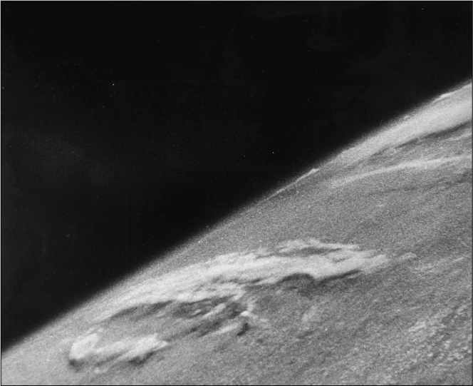
First photograph taken from space, October 24, 1946. Copyright 1946, Johns Hopkins University, Applied Physics Laboratory. Appears by permission.
The need was clear: the military and IC did not know how many Intercontinental Ballistic Missiles (ICBM) or long-range bombers the Union of Soviet Socialist Republics (U.S.S.R.) had in its arsenal. The U.S.S.R. government closely controlled its borders and communication systems, effectively closing its society to outsiders. As a closed society, little information was getting out, and gathering traditional human intelligence was difficult (NRO, 2013, p. 8). By 1960, it was feared that the U.S.S.R. had surpassed the United States in missiles and bombers; this was often defined as the “bomber gap” and the “missile gap” (NRO, 2013, p. 61).
In response, the United States, in the late 1940s and early 1950s, sent USAF planes over the U.S.S.R. on aerial photography missions. Eventually, the United States stopped the missions due to aggressive actions by the U.S.S.R., including shooting down several planes (Pedlow and Welzenbach, 1998, p. 2–4). The United States then developed high-altitude balloons and the U–2 reconnaissance aircraft to fly over and take images of U.S.S.R. territory. The reconnaissance balloon program, Project Moby Dick, operated in January and February 1956 and was canceled due to U.S.S.R. protests and, in any case, collected only one useful intelligence image of the Soviet Union (NRO, 2013, p. 8). The CIA developed the U–2 to fly at altitudes over 70,000 ft. It was thought that at this altitude, the U–2 would be able to fly above the range of radar and air-to-surface missiles (Pedlow and Welzenbach, 1998, p. 46). From 1956 to 1960, the U–2 made 24 missions over U.S.S.R. territory and imaged about 1 million mi2 or about 10 percent of its territory (NRO, 2013, p. 3, 61, 126). The U–2 program was tremendously successful in addressing policymakers’ needs for intelligence on the ground-situation in the U.S.S.R. For example, U–2 flights proved there was no “bomber gap,” enabling President Dwight D. Eisenhower to avoid overreacting to the perceived Soviet threat and tamp down growing tensions. On May 1, 1960, the U.S.S.R. shot down a U–2 flown by Francis Gary Powers. This event ended U–2 overflights of U.S.S.R. territory. Several months later, the United States successfully launched Corona, the Nation’s first photographic reconnaissance satellite, which returned more photographic images of U.S.S.R. territory in its first mission than what the entire 4 years of U–2 overflights had achieved (NRO, 2013, p. 3, 61).
Corona
Following the RAND studies, the USAF began work on an Advanced Reconnaissance System, code-named Weapons System 117L (WS–117L). The WS–117L considered various options for photographic reconnaissance. The October 14, 1957, launch of the Sputnik satellite by the U.S.S.R. spurred the military and IC to act. Part of the response was President Dwight Eisenhower formally endorsing the Corona Program in February 1958 as an independent program, separate from WS–117L, as a way to gather information from within the U.S.S.R. Eisenhower gave management responsibility to the Central Intelligence Agency (CIA) and USAF (NRO, 2013, p. 4–15). In 1961, the Corona Program was transferred to the recently established National Reconnaissance Office (NRO) within the DOD (NRO, 2013, p. 18, 75). The highly classified Corona Program was placed under cover of the Discoverer Program, an unclassified USAF scientific and engineering program, to conceal its existence. Since it is difficult to conceal rocket launches, early Corona missions were called “Discoverer missions” (NRO, 2013, p. 23).
In the 1950s, launching and controlling rockets to achieve the desired Earth orbit was a complex, highly technical endeavor. Explosions on the launch pad or shortly after liftoff, rockets going off course, and lost communications were common in-flight failures. What made it possible to launch a satellite into Earth’s orbit was advances made by the mid-1950s to the ICBMs. The size and weight of a small thermonuclear bomb are about the same as those of a satellite. Eventually, the Corona Program would use a Thor rocket as a first stage and an Agena rocket as a second stage (NRO, 2013, p. 18). To place a Corona satellite (fig. 37) in the polar orbit necessary to fly over the U.S.S.R., the satellite was launched from Vandenberg Air Force Base in California. This location on the coast of the Pacific Ocean was beneficial, as in cases of rocket failure, debris would fall harmlessly into the ocean (NRO, 2013, p. 36).
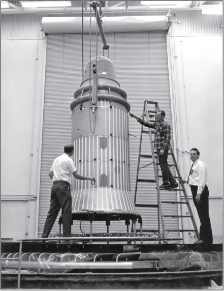
Black and white photograph of engineers readying a Corona (KH–4) satellite for launch. Photograph appears courtesy of the National Reconnaissance Office, Center for the Study of National Reconnaissance.
Adding to the challenges was the difficulty of designing and building a camera able to operate in the inhospitable conditions of outer space and return the exposed film to Earth. At the time, no object had ever been launched into space and safely returned to the Earth’s surface intact. For the Corona Program, a film-return capsule (fig. 38) was designed and constructed so that the exposed films would reenter Earth’s atmosphere and be captured midair near Hawai’i by a USAF C–119J airplane (fig. 39) flown by the 6593rd Test Squadron (NRO, 2013, p. 38).
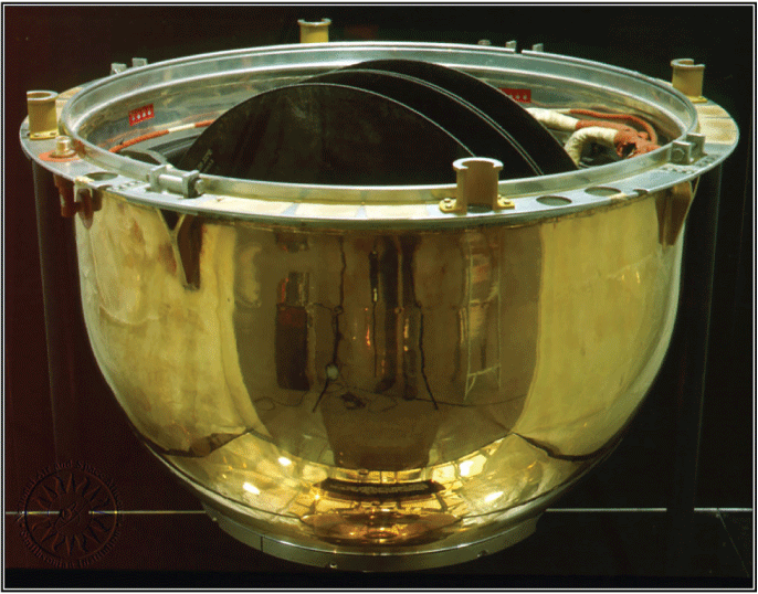
Photograph of a Corona satellite film-return capsule. The capsule is 2-feet (ft), 2-inches (in.) tall by 2-ft, 6-in. wide by 2-ft, 6-in. deep. This capsule is from the final Corona mission and was recovered on May 25, 1972. Photograph appears courtesy of the Smithsonian National Air and Space Museum.
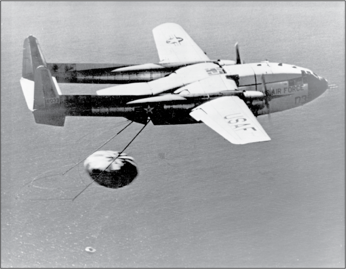
Photograph of a specially modified U.S. Air Force C–119J airplane recovering a Corona capsule returning from space. Photograph appears courtesy of the U.S. Air Force.
The first attempt to launch Corona occurred on January 21, 1959. While the rocket was on the launch pad, the upper-stage orientation rockets prematurely ignited and severely damaged the Thor rocket. Though not officially designated a Discoverer Mission, it is considered “Discoverer 0.” It would take the 14th launch attempt, referred to as Discoverer XIII, on August 11, 1960, to successfully launch and recover a film return capsule. The mission was a diagnostic flight that carried no film, but it did hold an American flag that was shown to President Eisenhower at a White House ceremony on August 15 (fig. 40).
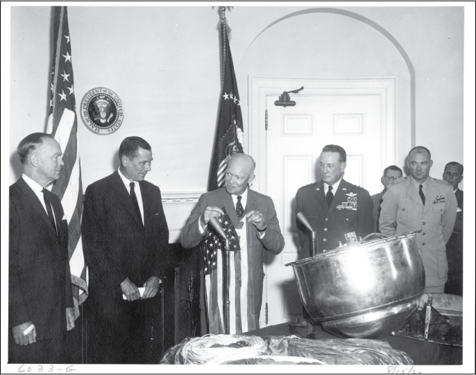
Black and white photograph taken on August 15, 1960, in which President Dwight D. Eisenhower holds the American flag carried in the Corona capsule retrieved from Discoverer XIII. Pictured left to right: Air Force Secretary Dudley C. Sharp, Secretary of Defense Thomas Gates, President Eisenhower, General Thomas D. White, and Colonel Charles A. Mathison. Photograph by Abbie Rowe appears courtesy of the Dwight D. Eisenhower Presidential Library, Museum, and Boyhood Home.
A week later, on August 18, 1960, the 15th Corona launch resulted in the first film successfully returned to Earth. Photographs of more than 1,650,000 mi2 of U.S.S.R. territory were acquired. Images over the United States were also collected for testing and engineering studies and to train image interpreters (fig. 41). The image resolution of the KH–1 camera carried on that mission was 35–40 ft. Image resolution is the size of the smallest object that can be observed. An image of the Mys Shmidta Airfield (fig. 42) in the northeastern U.S.S.R. is typical of the intelligence gathered in this first mission, where a runway and parking apron are visible. Even at this coarse resolution, image analysts identified 64 airfields and 26 surface-to-air sites in the imagery from this first mission (Ruffner, 1995, p. 2). The IC was thrilled with the images from the first Corona mission. According to Ruffner (1995, p. 2), the results of this first mission “stunned knowledgeable observers from imagery analysts to the President.” Figure 43 shows Miami, Oklahoma, and is typical of the engineering and test images acquired over the United States during Corona’s first mission. Later, the NRO collected engineering and test images to satisfy the USGS’s requests for images that could be used to revise topographic maps. This application is discussed later in this report.
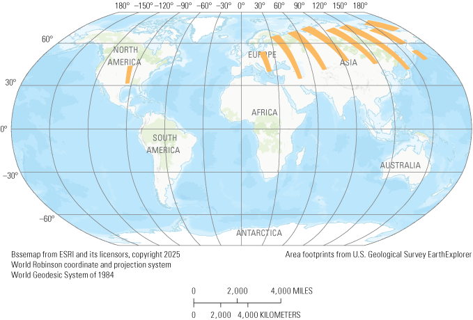
World map showing areas (orange) from which data on the United States and the U.S.S.R. were collected during Corona Mission 9009, August 18, 1960. The area footprints were downloaded from U.S. Geological Survey EarthExplorer (https://earthexplorer.usgs.gov/).
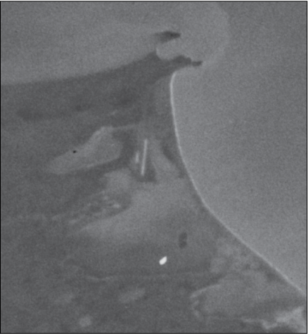
Satellite photograph of the Mys Shmidta Airfield in the northeast region of the Union of Soviet Socialist Republic from the first successful Corona mission, designated 9009, acquired August 18, 1960, KH–1 camera, image resolution of 40 feet (U.S. Geological Survey, 2017b).
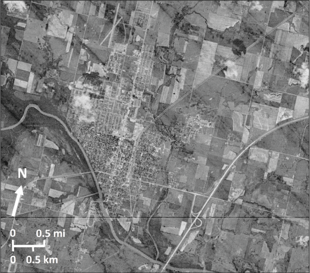
Satellite photograph of Miami, Oklahoma, acquired August 18, 1960, during the first Corona mission (9009). Domestic areas were acquired for engineering and test purposes. Scale is approximate due to off-nadir photograph (U.S. Geological Survey, 2017a).
The Corona Program operated from 1960 to 1972 and included 145 launches. Over 12 years, the Corona Program saw many improvements. The first Corona mission’s KH–1 camera had an image resolution of 35–40 ft, but within 12 years, the camera resolution improved to 6 ft through successive KH–2, KH–3, KH–4, KH–4A, and KH–4B missions, as shown in table 1. A variety of camera systems were used. The KH–1, KH–2, KH–3, and KH–6 satellites carried a single panoramic camera. The KH–5 satellite carried a single-frame camera (KH–5). The later systems (KH–4, KH–4A, and KH–4B) carried two panoramic cameras with a separation angle of 30 degrees, with one camera looking forward and the other looking aft to achieve stereoscopic images, which were beneficial in letting analysts view the land surface in three dimensions (USGS, 2018a).
Table 1.
Corona Program missions and associated information (USGS, 2018a).Corona satellites also included a stellar camera for positioning and navigation alongside index cameras with a lower resolution and a broader field of view to place the higher resolution images in context. Figures 44 and 45 are examples of Corona imagery collected over the United States during later missions, when the resolution was 6–9 ft. By the end of the program, each satellite could carry 16,000 ft of film, capturing about 8.4 million square nautical miles (nmi2) of area compared to the 3,000 ft of film the first mission carried. The program used approximately 2 million ft of film, representing a cumulative coverage of over 750 million nmi2, which is about 220 times the land area of the United States.
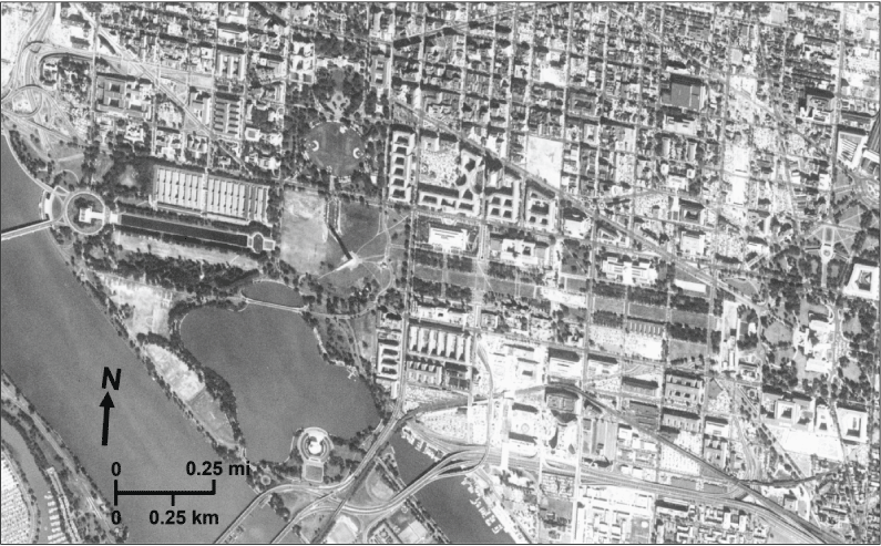
Corona satellite image of the National Mall, Washington, D.C.; Mission 1101, KH–4B camera. The image was acquired September 25, 1967, and the image resolution is 6 feet. The scale shown is approximate because the image is off-nadir (U.S. Geological Survey, 2017e).
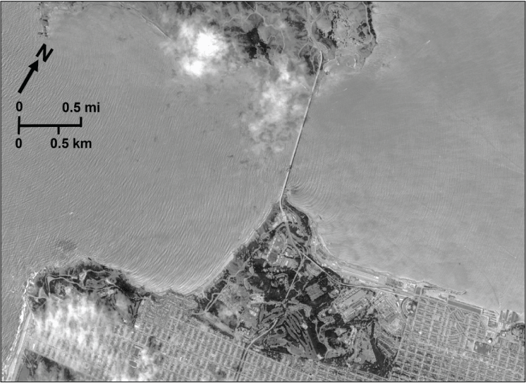
Corona satellite image of the Golden Gate Bridge, San Francisco, California; Mission 1023, KH–4A camera. The image was acquired June 8, 1965, and the image resolution is 9 feet. The scale shown is approximate because the image is off-nadir (U.S. Geological Survey, 2017c).
The Corona Program resulted in many “firsts” in history:
-
• first photoreconnaissance satellite in the world,
-
• midair recovery of a vehicle returning from space,
-
• mapping of Earth from space,
-
• stereo-optical data from space,
-
• multiple reentry vehicles from space,
-
• reconnaissance program to fly 100 missions, and
-
• reconnaissance satellite program to be declassified (NRO, 2013).
McDonald (1997) reported that 4.6 percent of Corona’s film was acquired over the United States “in support of engineering and domestic mapping programs” (p. 70). Domestic images were acquired to ground-truth what was observed in denied areas. Known features in the United States could be measured and compared with similar features in other countries (McDonald, 1997, p. 71). The domestic images were used to aid and train image interpreters. The USGS was the largest civil-agency user of Corona data (Baclawski, 1997).
The Corona Program cost $850 million, with the average mission cost ranging from $7 million to $8 million (NRO, 2013, p. 121).
Samos
The Samos Program also emerged from the WS–117L Program and was originally envisioned as a technology that would transmit images electronically like a television transmission. The developers transitioned to a film-return system like the one used by Corona when that endeavor proved difficult. It was thought that Corona would be an interim system until Samos’ development was complete. Samos achieved poor results and was canceled in 1961 after several launches. The NRO incorporated the Samos camera systems into later Corona missions. The National Aeronautics and Space Administration (NASA) was allowed to integrate the Samos camera systems into its Lunar Orbiter satellites to image the Moon: another example of military-developed technology being used by a civilian agency (Hall, 2001). NASA launched five Lunar Orbiters with a modified Samos camera (Mitchell, 2012, p. 17–18). On August 23, 1966, the Samos-developed camera took the first photograph (fig. 46) of the Earth from the Moon (Hall, 2001). Cloud (2002) reports that similar technology transfers from the NRO to NASA aided the Mariner and Voyager programs.
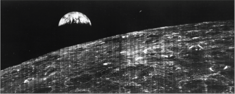
First photograph of the Earth from the Moon as captured with camera technology developed for the Samos mission and adapted to fly on the first Lunar Orbiter missions. Photograph appears courtesy of the National Aeronautics and Space Administration.
Argon, Lanyard, and Gambit
Three other systems were under development and operated under the Corona Program. While separate from Corona, these systems are often grouped together because they overlap in time and share common systems. The NRO developed Argon to support the U.S. Army’s need for mapping data, particularly geodetic information over the U.S.S.R., where the United States had little up-to-date mapping information (NRO, 2013, p. 46). Six missions with its KH–5 camera were flown from May 1962 to August 1964 (table 1). The results were described as mediocre (Ruffner, 1995, p. xv). Lanyard was meant to be the high-resolution successor to Samos but achieved limited success and was canceled after three launch attempts and only one successful launch with its KH–6 camera (table 1).
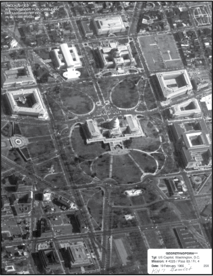
Gambit (KH–7 camera) satellite photograph of the U.S. Capitol Building, Washington, D.C., February 19, 1966. Digital photograph appears courtesy of the National Reconnaissance Office (NRO), Center for the Study of National Reconnaissance (NRO, 2000).
Corona was successful in imaging large areas and gave analysts an unprecedented view of areas denied to the IC. To meet the need for high-resolution images sufficient to identify individual airplanes, ships, and other items of interest to intelligence analysts, the NRO developed the GAMBIT 1 Program and launched 38 missions from July 1963 to June 1967 (fig. 47). The KH–7 camera on these missions achieved an image resolution of 2–3 ft (NRO, 2011a). The NRO operated the GAMBIT 3 Program from July 1966 to April 1984, with 54 missions. Its KH–8 camera had an image resolution of less than 2 ft (NRO, 2011b). As of the publication of this report, KH–8 imagery is not available to the public.
Hexagon
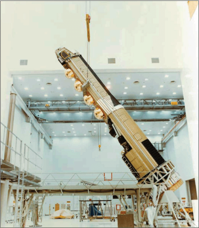
Photograph of Hexagon satellite being prepared for launch. Photograph appears courtesy of the National Reconnaissance Office, Center for the Study of National Reconnaissance.
The Hexagon Program succeeded Corona in its broad area-search missions, added a mapping mission, and operated from June 1971 to April 1986. Over the program’s duration, 19 satellites (fig. 48) reached orbit in 20 attempts, Mission 1220 experienced a launch failure seconds after liftoff (table 2), and 12 missions included a mapping camera. Hexagon’s KH–9 panoramic camera’s image resolution was 2–3 ft, and the mapping camera’s resolution was 30–35 feet. Hexagon included multiple film-return buckets and 60 mi of film on each satellite, allowing for longer missions and achieving a nearly continuous presence in orbit (NRO, 2011c). During the life of the program, 877 million mi2 of area-imagery was acquired (NRO, 2011c). Figures 49 and 50 provide examples of Hexagon images. Table 2 lists the Hexagon missions.
Table 2.
Hexagon Program missions (USGS, 2018c).[The decay date is the date the satellite was de-orbited]
While developed, launched, and operated to serve military and intelligence needs, the Corona and Hexagon satellites’ ability to capture images of large areas at spatial resolutions suitable for mapping would also fulfill the imagery needs of the USGS in its topographic-map revisions and other applications.
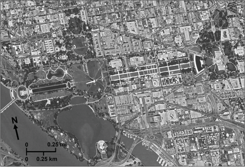
Hexagon satellite image of the National Mall, Washington, D.C., Mission 1215, KH–9 camera. The image was acquired June 13, 1979, and the image resolution is 2–4 feet. The scale shown is approximate because the image is off-nadir (U.S. Geological Survey, 2023d).
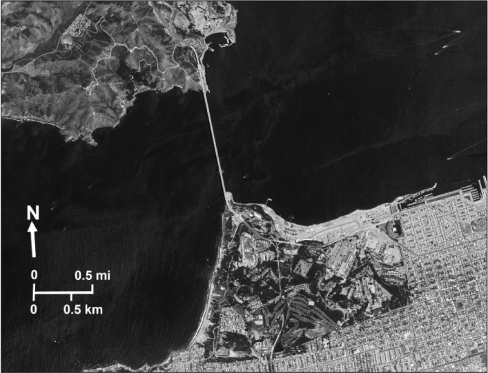
Hexagon satellite image of the Golden Gate Bridge, San Francisco, California, Mission 1215, KH–9 camera. The image was acquired June 8, 1979, and the image resolution is 2–4 feet. The scale shown is approximate since image is off-nadir (U.S. Geological Survey, 2023c).
Adjudicating Collection Requests
Deciding which areas to collect photographs from using Corona and Hexagon satellites required close collaboration between intelligence and military professionals in multiple agencies and military commands. For this task, in August 1960, the Director of Central Intelligence (DCI) established the Committee on Overhead Reconnaissance (COMOR) under the U.S. Intelligence Board (USIB) “to coordinate the development of intelligence requirements for reconnaissance missions over the Soviet Union and other denied areas” (Ruffner, 1995, p. 41–43). By 1967, increased collaboration and coordination in exploiting imagery for military and intelligence purposes gained importance. In response, the USIB added the responsibility for exploitation coordination and collaboration to COMOR and created a new organization: the Committee on Imagery Requirements and Exploitation (COMIREX). COMIREX “provides staff support to, and acts for, the USIB in development and implementation of national-level guidance for overhead imagery collection and exploitation” (CIA, 1976). COMIREX would operate for the rest of the Corona program and the duration of the Hexagon flights (NRO, 2013, p. 123).
The USGS and other Federal civil agencies would come to benefit from Corona and Hexagon images and would find many applications and missions to support. It would be to COMIREX that the USGS would submit its requests for image collection to support its map revision program, as discussed later in this report.
Declassification and Public Access
In 1990, U.S. Senator Albert Gore asked the CIA and the NRO to consider releasing environmental data to augment civilian earth science studies. CIA Director Robert Gates agreed, and in January 1992, commissioned the Environmental Task Force to review classified systems, data, and archives for environmental data. At the same time, a Classification Review Task Force considered the declassification of satellite imagery from the early reconnaissance systems. The reviews concluded that “the first group of satellites flown in the 1960s offered unusual and valuable information for scientists, scholars, and historians” (Baker and Zall, 2020).
In 1995, President William Clinton declassified Corona, Argon, and Lanyard and directed that a copy of the film be sent to the USGS for the purpose of public availability; the original copy of the film was sent to the National Archives and Records Administration (White House, 1995). The USGS Earth Resources Observation and Science (EROS) Center in Sioux Falls, South Dakota, makes the images available via the USGS EarthExplorer website (https://earthexplorer.usgs.gov/) under the dataset name “Declass 1 (1996)” (USGS, 2018a). In 2002, GAMBIT (KH–7) imagery was declassified by Executive Order 12951 (White House, 1995) and is available via the USGS EarthExplorer website under the name “Declass 2 (2002)” (USGS, 2018b). EROS made a portion of the Hexagon imagery publicly available on EarthExplorer as “Declass 2 (2002)” (USGS, 2018b), with additional imagery made available as “Declass 3 (2013)” (USGS, 2018c).
Declassified imagery has been used in a wide range of applications. Recent examples include—
-
• searching for Roman archeology in the Middle East (Casana and others, 2023),
-
• geomorphological reconstruction of the urban landscape in Iraq (Forti and others, 2023),
-
• detecting liquefaction manifestations due to an earthquake (Taftsoglou and others, 2023), and
-
• the study of barrier-island dynamics in the United States (Fisher and others, 2023).
Path to Civil-Agency Use
By the early 1960s, scientists used aerial photography for applications beyond topographic mapping, such as agriculture (Monmonier, 2002, Campbell, 2008, p. 88), urban planning (Manji, 1968), land-use analysis (Werle, 2016), soil surveys, dam-site planning, flood and erosion studies, and road planning (Lundahl and Brugioni, 1985). Howe (1958), in writing about locating groundwater, also identified several more applications: geologic investigations, hydrographic research, and mineral exploration. The leap from analyzing photography from airplanes to photographic images from satellites in Earth’s orbit did not prove to be a large jump.
Photography from space has several benefits. First, large areas can be collected in a single image in a single day. During the first Corona mission (9009; table 1) on August 18, 1960, imagery for about 162,000 mi2 of the United States, an area approximate in size to the State of California (fig. 41), was collected for engineering and test purposes, a common practice in subsequent missions (Richelson, 2011). It likely would have taken months to collect imagery of the same area using aerial photography. Observations of a large area collected simultaneously, termed a “synoptic observation,” provide for the analysis of situations that fluctuate over time, as with floods and wildfires (Brugioni, 1970).
By the end of the 1960s, several concurrent activities led the USGS to open a secure facility to use the classified Corona photographic images for the bureau’s mapping mission (fig. 51). Today, the term Sensitive Compartmented Information Facility, or “SCIF,” denotes such a facility. By the mid-1960s, broader applications of Corona imagery, beyond intelligence and military requirements, were recognized and documented by the U.S. Army Engineer Topographic Laboratory (ETL), the CIA, and the National Photographic Interpretation Center (NPIC) (White House, 1968a). As documented in this report, a long-established collaborative relationship existed between the USGS and the military in the mapping sciences and other Earth science disciplines—the USGS’s use of Corona imagery naturally developed from these prior collaborations. Figure 51 lists key dates and events in the path toward civil agency use of Corona and later Hexagon images.
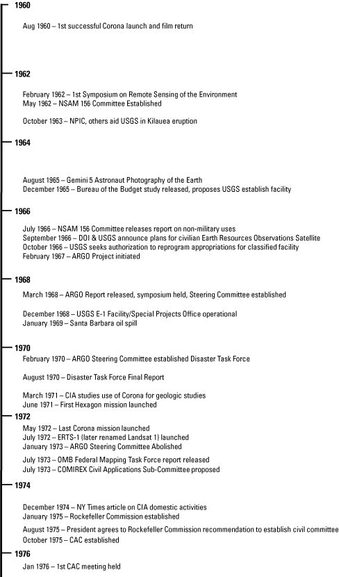
Timeline depicting activities, key dates, and events related to Federal civil agency satellite use, displayed in 2-year intervals, between 1960 and 1976.
Policy Considerations
On May 26, 1962, less than 2 years after the first successful Corona mission, President John F. Kennedy issued National Security Action Memorandum 156 (NSAM 156) to the Secretaries of State and Defense, the Directors of Central Intelligence, NASA, and the Arms Control and Disarmament Agency. President Kennedy directed the Department of State to lead a committee to look at “what constitutes legitimate use of outer space, and in particular the question of satellite reconnaissance” (White House, 1962). International negotiations on disarmament and considerations of peaceful uses of outer space made it necessary for the President to establish policies on the use of satellite reconnaissance, which, by this time, had become operational.
In 1966, at the request of the Bureau of the Budget (BOB), today’s Office of Management and Budget (OMB), Director Charles Schultze and Presidential Science Advisor Dr. Donald F. Hornig (fig. 52), the NSAM 156 committee considered nonmilitary use of Corona and other classified remote sensing systems such as the U–2 aircraft. Of particular interest to Schultze and Hornig were discussions NASA and NRO were having over their respective Earth-observing missions. As part of the Gemini Program, NASA astronauts, in 1965 and 1966, used handheld cameras to acquire about 1,100 photographs in color and color infrared (fig. 53), from space, of geologic, oceanic, and meteorologic targets (Mack, 1990, p. 40).
Gemini photographs demonstrated that images from space, when not obscured by clouds, could be used to delineate cultural features for topographic mapping (Doyle, 1973, p. 315). As part of a collaboration with NASA and the Raytheon Corporation, the USGS prepared a 1:1,000,000-scale photomosaic of Peru using 12 photographs from the Gemini 9 mission that proved, for many purposes, better than existing maps (MacKallor, 1967). NASA was also planning subsequent Earth-observing missions, including Landsat, which is discussed later in this report (Mitchell, 2012, p. 25). The Gemini photography’s spatial resolution was comparable to Corona photography, which caused concern among some in the defense and intelligence communities because the data were not classified and might reveal military and intelligence information to adversaries (Mitchell, 2012, p. 27).
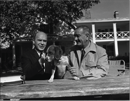
Photograph of Presidential Science Advisor Dr. Donald F. Hornig and President Lyndon B. Johnson with one of the President's beagles.
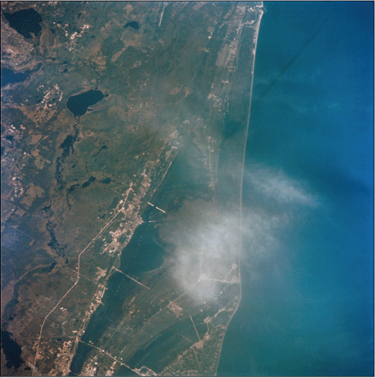
Photograph of the Kennedy Space Center, Merritt Island Complex on the east coast of Florida, taken during the Gemini VII Mission on December 6, 1965. Photograph appears courtesy of the National Aeronautics and Space Administration.
In July 1966, the NSAM 156 committee issued a report titled “Political and Security Aspects of Non-Military Applications of Satellite Earth-Sensing.” The committee addressed the use of U–2 and Corona imagery by nonmiliary agencies and made the following recommendation, which is number 5 in the report:
“NASA and other appropriate agencies should carefully consider the relative merits and costs of aerial and other possible alternatives to various space-borne earth-sensing programs in terms of practical political interest as well as cost effectiveness. Similarly, the respective merits of manned and unmanned satellites will of course require consideration. To assist in deciding these questions, NASA and other appropriate government personnel should be permitted to use selected U–2 and KH–4 photography most of which is now code word classified, to advance its studies of non-military earth sensing applications.” (DOS, 1966).
This recommendation opened the door for Federal civil agencies, such as the USGS, to use Corona images.
Budget Process
In 1965, the BOB commissioned a study on the potential use of Corona imagery for civilian mapping. That study reported that classified imagery could meet civilian agencies’ mapping needs. One of the recommendations was for the USGS to establish a secure facility to use Corona imaging for its map-revision mission (CIA, 1977a). In remarks made in 1995, Lowell Starr, who, as a USGS cartographer in the mid-1960s, helped develop the processes for using Corona photographic images for mapping and later became a USGS senior executive, stated: “The study essentially served as the springboard for getting the civilian community involved with the program” (Day and others, 1998, p. 212). Ondrejka (1997) credits the CIA, the Defense Intelligence Agency (DIA), and the BOB for taking the initiative in 1966 to establish a civil mapping facility and permit the USGS, the U.S. Forest Service (USFS), and the Environmental Protection Agency (EPA) to use Corona photography coverage for their mapping purposes (p. 155–156).
Following the December 1965 release of the BOB report, the USGS sought and obtained appropriations as part of its fiscal year (FY) 1968 budget to build a secure facility that, as Turner noted, “became the national depository for classified imagery of the United States” (CIA, 1977a). In an October 25, 1966, memorandum, USGS Director William T. Pecora (fig. 54) wrote to the Assistant Secretary of Mineral Resources, his superior at the Department of the Interior (DOI), that “The Bureau of the Budget has been advised informally of our intention to reprogram within the 1968 topographic mapping budget to finance initial steps to establish a classified mapping activity.” (W.T. Pecora, written commun., 1966). The CIA briefed the House Appropriations Committee in late January 1967 to support the USGS budget request (CIA, 1967). According to a CIA report, Congress gave its approval in February 1967 (CIA, 1977a). This decision followed the release of the BOB mapping study, which recommended that the USGS establish such a facility.
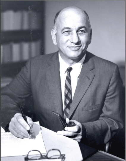
Photograph of U.S. Geological Survey (USGS) Director William T. Pecora, 1965. Photograph appears courtesy of USGS Denver Library Photographic Collection.
The USGS spent $300,000 to build the facility. It was built, staffed, and occupied after only 13 months (Day and others, 1998, p. 212). That facility, often referred to as the “E–1 building,” opened in December 1968 (USGS, 1969) in Isaac Newton Square, a commercial office park in Reston, Va. (fig. 55). In some documents, the facility is referred to as the Special Projects Office (SPO), perhaps to obscure the classified nature of the data analyzed within the facility. The USGS established a new organization, the Special Mapping Office (SMO), which was later renamed the Special Mapping Center (SMC). Today, the successor organization is the USGS National Civil Applications Center. The facility was specially designed to use classified intelligence and military imagery. As Turner noted, the SMO hosted employees from civilian agencies such as the USFS and the EPA (CIA, 1977a).
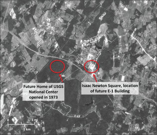
Corona satellite image showing the location of the U.S. Geological Survey (USGS) E–1 building and the future location of the USGS National Center, Reston, Virginia; Mission 1101, KH–4B camera (table 1). The image was acquired September 25, 1967. Image resolution is 6 feet. The scale shown is approximate because the image is off-nadir (USGS, 2017d).
Scientific Collaboration
Kīlauea volcano on the Island of Hawaiʻi erupted several times in the early 1960s. The USGS sought and received technical assistance from several different military and intelligence units. Moore and Koyanagi (1969) acknowledge receiving air reconnaissance support from the Hawai'i Army National Guard for the October 5–6, 1963, eruption (p. C1). What they did not, or perhaps could not, report on, because the support was classified at the time, was other military assistance that they and others in the USGS received. In unclassified correspondence between the USGS Director, the USGS Hawaiian Volcano Observatory, the USGS MGB, and the USACE, from June to December 1962, released by the CIA in 2000, it appears the USACE was prepared to support infrared surveys of the volcano using military aircraft (CIA, 1962). A letter to USGS Director Thomas B. Nolan dated August 27, 1962, references correspondence Nolan wrote to the Director, Geodesy, Intelligence, Mapping Research and Development Agency (GIMRADA), which was under the USACE. Later, GIMRADA would support Project ARGO, an effort to study civil agency applications of Corona data initiated by the President’s Science Advisor, as discussed later in this report (White House, 1967). One letter refers to the data as having the security classification “Confidential” (CIA, 1962).
Of particular interest is a now-declassified staff study released by the CIA in 2000 that proposes that the NPIC aid in the collection of data “which could serve as training material in training multisensory photo interpreters” (CIA, 1963a). Certain parts of the document were redacted before its 2000 release. An item of note is that the USGS would reimburse part of the cost of the analysis, but it is evident in the study plan that the NPIC would bear most of the cost. The plan references the use of naval aircraft, but other data sources are redacted. Moore and Koyanagi make no mention of the use of infrared imagery. The NPIC would have had experience analyzing photography from the U–2 and likely other military reconnaissance aircraft and the Corona satellite. Infrared data were apparently collected by the U.S. Army.
The CIA released (at the same time as the other documents in 2000) an unclassified press release from the University of Michigan’s Institute of Science and Technology (IST). In the release, the IST states that the Army provided the infrared instrument and that the work was sponsored by the USGS (CIA, 1963b). In 2014, the CIA released a copy of an article authored by two USGS scientists, a scientist from the IST, and an author from the Aero Services Corporation titled “Infrared Surveys of Hawaiian Volcanos” that was published in the journal “Science” in 1964. The first page of the released document is an NPIC routing slip, and the second page appears to be a memorandum with the entire page, except for the phrase “Memorandum For,” redacted (CIA, 1964). While it would be speculation to guess what was written on the memorandum, it can be safely presumed that the topic was of interest within the NPIC. While it is conceivable that the imagery was shared with IST scientists because it received the security classification “Confidential,” Brugioni, (1970, p. 60–61), in a then-classified article states that the NPIC and the USGS “combined forces for an aerial infrared survey of Hawaii.”
The infrared interpretation techniques developed in this project were used to monitor the eruption of Surtsey, an Icelandic volcano, in 1963. Later in this report, IST contributions to the development of the Landsat satellite’s multispectral sensor are described. The USGS, the military, and the IC continue, to this day, working together monitoring volcanos across the globe (Young, P., 2023). While at times the study saw the military assisting the USGS (fig. 5), the military—based on their involvement—appears to have benefited from analyzing the volcano imagery, so both civil and military sectors benefitted from this project (fig. 7).
In 1970, the CIA experimented with the feasibility of using Corona images for a geologic assessment. Panchromatic and color film were used. The study had three objectives:
-
1. Evaluate the information content of color versus black and white film type.
-
2. Evaluate the potential of the Corona system for resource exploration.
-
3. Perform sufficient analysis to indicate the potential advantages of color photography for geographic and economic intelligence purposes” (Ruffner, 1995, p. 321).
In its March 1971 report, the study came to three conclusions:
-
1. Effective photogeologic mapping can be achieved using the Corona system.
-
2. The value of color cannot be overstated.
-
3. The Corona system represents an essential breakthrough for national resource exploration (Ruffner, 1995, p. 356–357).
A private-sector company undertook the study for the CIA. It is uncertain what, if any, knowledge the USGS had of the study, but it does indicate that the IC was considering nonmilitary applications of Corona (Ruffner, 1995, p. 317–357).
Arthur C. Lundahl, the founding and longtime director of the NPIC, recognized the value of Corona for civilian applications and promoted sharing the data with Federal civil agencies. He shared this view with the DCI, under whom he served, and with the President’s Science Advisor (Brugioni and Doyle, 1997, p. 163–164). Later, Lundahl promoted using aerial and space imagery for emergency response, the management of natural resources, environmental protection, natural disaster prediction, and disaster response (p. 165). The NPIC would later serve as a model for the application of imagery for civilian uses, particularly disaster response (Lundahl and Brugioni, 1985).
White House Coordination
In 1967, Donald F. Hornig, Special Assistant to the President for Science and Technology, established what came to be known as Project ARGO to investigate the uses and potential applications of Corona images by Federal civil agencies. In his February 3, 1967, memorandum to the Secretaries of Interior, Agriculture, and Commerce, and the administrators of NASA and the [U.S.] Agency for International Development, Hornig laid out a detailed plan to study satellite photography for Earth-resource information. His memorandum started with the following statement: “In the past year, more and more interest has been developing in the potential use of satellite-borne sensors for earth resource and economic survey and there has been discussion about satellite systems to collect data in support of agency missions” (White House, 1967). In addition to the NSAM 156 committee’s report and the BOB mapping study, the latter of which he initiated, Hornig also knew about a 1966 military geology study undertaken by the ETL and broader applications for the imagery found by the CIA, the NPIC, and the DIA (White House, 1968a).
Hornig’s idea was for the agencies he addressed to name staff who could investigate the Corona photography already collected to make better program-planning decisions. At this point, the USGS was already planning to use Corona photography to update its topographic maps. The USACE provided space in one of their contractor’s facilities, Autometric, Inc., in Alexandria, Va. Autometric supported GIMRADA through a contract with the USACE, who were already reviewing Corona data. GIMRADA surveyed Africa, to include producing a giant photomosaic of the African continent from Corona imagery that was collected from 1962 to 1964 and did the same for Antarctica and the Arctic Ocean Basin (Cloud, 2002). In addition to the USACE, the NPIC, DIA, and U.S. Army Map Service (AMS) provided technical assistance (White House, 1968a). Hornig laid out three objectives:
-
1. “To evaluate the existing aircraft and satellite photography and describe its usefulness for physical resource surveys and its bearing on the design of future systems.
-
2. To develop a cadre of civilian agency personnel who will know what information is available and how the photography can be used.
-
3. To produce as a byproduct a resource inventory of typical areas of interest to AID [U.S. Agency for International Development] to show what might be done with the existing photography and to determine whether such a program is worth continuing” (White House, 1967).
The Project ARGO team began work in July 1967 and was completed by early 1968. The effort was meant to be a quick study to identify information and uses that could be gleaned from the imagery that would be useful for agency missions but did not detail acquisition or exploitation costs. The team of civilian scientists had at their disposal 2,178 images from the KH–4, KH–5, and KH–7 missions and another system that was redacted in the executive summary (White House, 1968a). The team started with a study in South America—an area of special interest to the U.S. Agency for International Development (USAID)—and later in the United States, where maps, other photography, reports, and personal experience were readily available to serve as ground truth to verify information interpreted from the Corona imagery.
The study of South America investigated surface drainage, engineering and structural geology, vegetation, surficial materials, surface configuration and landforms, and climatology. Topics studied in the United States were more detailed and comprehensive because ground-truth data were readily available; these topics are shown in table 3. The product is a four-volume report:
-
• Volume I is a declassified executive summary that was publicly released (White House, 1968a).
-
• Volume II is a collection of individual investigators’ reports.
-
• Volumes III and IV are atlases containing maps, graphics, and images.
The Project ARGO team agreed that the current systems are useful to the agencies that reviewed the data. However, the cost of exploitation, which civil agencies would bear, was not considered. It was assumed that the IC would pay for the cost of data collection. The lower resolution index imagery was helpful for broad area, synoptic views that could be used for regional planning. The team saw major advantages in satellite photography, especially when using the large-area coverage collection possible through use of a space sensor.
Project ARGO reports included mapping as one of the topics covered. The report states that there is little geodetic value of the imagery in the United States, where large amounts of ground truth and survey control exist, but the imagery could generate photogrammetric control in parts of the world where little geodetic control was established. The Argon satellite described previously was designed to support the Army’s geodetic mapping needs, but perhaps its imagery was not released to the Project ARGO team because of the sensor’s lackluster performance. The project team found that KH–4 and KH–7 imagery provided high-quality information on landforms, drainage patterns, physiography, hydrologic delineation, and forest delineation—all features shown on USGS topographic maps (White House, 1968a).
One of Hornig’s expected outcomes for Project ARGO was symposiums. A Project ARGO Symposium was held on March 6, 1968, in the NPIC auditorium. Topics listed on the agenda were hydrology, agriculture land use, forestry, land use and acreage, geology, geography, oceanography, map and map production, and USAID interests. While the names of presenters are redacted, the geography and geology briefings were done by USGS individuals who are likely not the same people because the scientific disciplines are separate (White House, 1968b).
ARGO Steering Committee
While Project ARGO ended with the publication of its four-volume report, the ARGO Steering Committee, initially established to coordinate the project, persisted. On March 5, 1968, the Special Assistant to the President for Science and Technology wrote to the Secretaries of Agriculture, Commerce, Interior, and Transportation, the administrators of the USAID and NASA, and the Director of the Office of Emergency Planning to inform them of the continuation of the ARGO Steering Committee as a standing committee with three tasks:
-
“1. Collect and consolidate the needs that each of you might have for some photography from the current systems,
-
2. See that these needs were made known to the intelligence community and
-
3. Discuss procedures for handling classified photography for these purposes with the community” (White House, 1968c).
The minutes of the July 10, 1968, ARGO Steering Committee included a detailed report from the USGS on its plans for a classified map-production facility. The USGS hoped the Reston, Va., facility would be operational by October 1, 1968, with an initial staffing level of 47 people, including 5 guards, with plans to grow over 5 years to 115 employees. Initially, the facility would be used to update the 1:250,000-scale topographic maps for the country in 5 years, with eventual plans to revise cultural details on the 1:24,000-scale maps. The USGS also announced plans to map Antarctica at a scale of 1:3,000,000 (White House, 1968d).
At the December 9, 1969, ARGO Steering Committee meeting, the USGS representative presented work done by the SMO on planning the trans-Alaska pipeline. KH–4 imagery was used to plan the route north of Fairbanks (fig. 56), where little information was available. Of note was the time savings. The pipeline mapping effort took 1 month to complete, whereas it may have taken 2–3 years to complete by conventional means (CIA, 1969c).
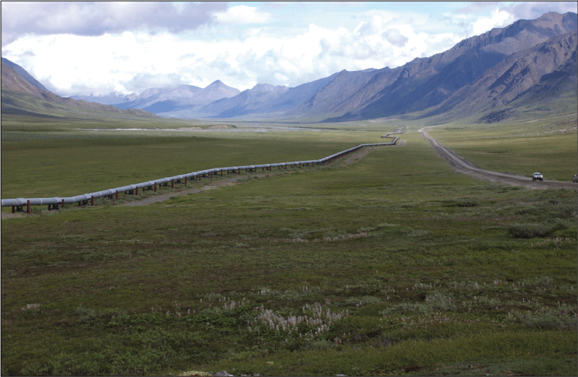
Photograph of a section of the trans-Alaska pipeline, June 20, 2007. Photograph by David Houseknecht, U.S. Geological Survey.
The committee continued to meet until the Science Advisor position was abolished by President Richard Nixon in 1973. Later, in 1973, National Security Advisor Henry Kissinger drafted a memorandum that formally abolished the ARGO Steering Committee and proposed that it be replaced with a Civil Applications Subcommittee under COMIREX. The draft of that memorandum was reviewed by various offices within the CIA, and it was proposed that the DCI concur with Dr. Kissinger’s draft memorandum as amended. Kissinger stated that “a routine mechanism, not available via ARGO, is required to receive, evaluate, and satisfy requests for new data” (CIA, 1973). His proposed subcommittee would be chaired by a representative from the DOI. One comment, made on an official routing slip dated August 28, 1973, proposed that questions be raised on the increased cost incurred through civil-agency use; however, the COMIREX Chairman, in a memorandum, acknowledges that “the needs of civil agencies have generally been met as byproducts of satellite engineering operations over the U.S. or on an ad hoc basis as circumstances permitted.” (CIA, 1973)
No documentation has been found to explain the name “ARGO.” One hypothesis is that the name is derived from Greek mythology. In 1960, the DOD formed JASON, an independent group of scientists who could advise the Department on science and technology topics. The group’s name, JASON, comes from the Greek myth of Jason and the Argonauts, in which Jason is the hero of the story and represents a man on a quest. The Argonauts were his warriors, and together, they set out on the Argo, Jason’s ship, to find a treasure: the “golden fleece” (Jacobsen, 2016, p. 126). Perhaps “ARGO” was selected as a name because this group of Federal scientists were “on a quest” to study the use of imagery from Corona (a “ship” of sorts) and informally associate the Project ARGO with the JASON advisory group.
In 1993, Vice President Albert Gore established “MEDEA” with scientists from the IC, Federal civil agencies, and academia to study the use of classified remote-sensing images for scientific purposes. As Baker and Zall (2020) wrote, “The name MEDEA was chosen, not as an acronym, but to complement the name of another government advisory group, JASON, whose name had come from the Greek myth of Jason, Medea, and the Argonauts.” In the myth, Medea helps Jason in his quest to find the golden fleece. MEDEA could be considered a successor to Project ARGO.
Disaster Response
Based on experiences with aerial photography, there was early recognition that satellite imagery would benefit disaster response and recovery. The January 28, 1969, oil spill from an offshore oil rig in the Santa Barbara Channel resulted in a significant Federal Government response, part of which involved use of a U–2 airplane to acquire aerial photography of the spill (fig. 57). Secretary of the Interior Walter Hickel requested assistance from President Nixon’s Science Advisor, who may have been interacting with the ARGO Steering Committee. A U–2 plane was dispatched to the area to collect both black and white and color aerial photography of the spill. The NPIC-analyzed imagery showed contaminated beaches, damaged marinas, and kelp beds differentiated by oil. A copy of the film went to the USGS (Lundahl and Brugioni, 1985). The USGS used the U–2 film to determine the extent of the oil slick (Pedlow and Welzenbach, 1998). Cropped and enlarged areas of prints were deemed unclassified, making them more readily available (CIA, 1969a). Clark and Hemphill (2002) contend that this was the first peaceful use of the U–2 (fig. 5).
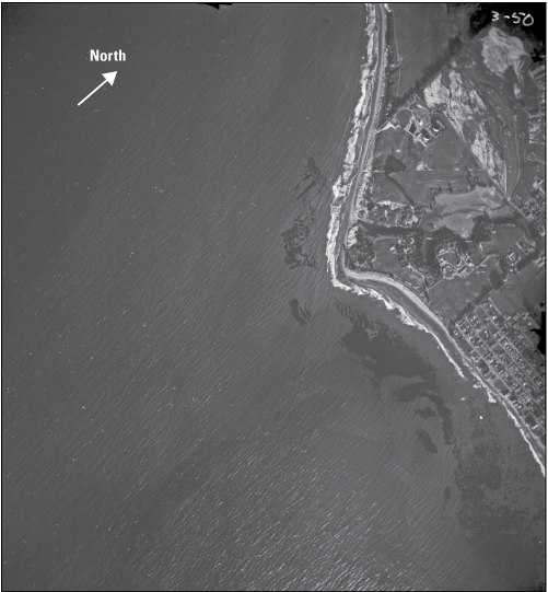
U–2 plane photograph of the Santa Barbara oil spill. Photograph 3–50, roll 3. The image was acquired March 7, 1969, off Coal Oil Point, California. The scale of the original 9-inch by 9-inch photograph is 1:20,000. Photograph appears courtesy of the U.S. Government, retrieved from the University of California Santa Barbara Library (https://mil.library.ucsb.edu/ap_images/project-02599/).
In August 1969, Hurricane Camille, a Category 5 hurricane, affected large areas of the southeast United States, Tennessee, Kentucky, and Virginia, resulting in 256 deaths and approximately $1.4 billion in damage (Senesac, 2020). A U–2 aircraft was sent to collect photography of the damaged areas, and CIA analysts at the NPIC documented the damage (Lundahl and Brugioni, 1985).In 1970 the ARGO Steering Committee established a Disaster Support Task Force to study aerial photography and other imagery for use in disaster response activities. The Task Force first met on February 17, 1970, at the USGS SPO (White House, 1970a). In March 1970, the Task Force Chairman requested KH–4 imagery of the Florida and Gulf Coasts ahead of the Hurricane season. In a cover memo transmitting the request to the COMIREX, the ARGO Steering Committee Chair stated that “The KH–4 photography makes an excellent data bank of predisaster information against which post-disaster aerial photography can be interpreted to determine the extent and severity of the disaster area” (White House, 1970b). The USGS advocated using the U–2 since the 70,000-ft flying altitude provides a per-frame coverage of a 5- by 10-mi area at a scale of 1:35,000. Flying at a lower altitude would require many frames of photography, and integrating the images into a single mosaic was a difficult process (White House, 1970c).
The task force issued its final report on August 3, 1970, titled “Application of Remote Sensing Imagery in Natural Disaster Effects Assessments” to the ARGO Steering Committee. While this final report focused extensively on using aircraft and aerial photography to collect post-disaster data and information, classified KH–4 imagery was acquired and used as a predisaster baseline ahead of the 1970 hurricane season. The use of the USGS SPO to hold the meetings indicates that these were likely classified meetings. The report recommended that the USGS SPO function “as the focus of working activities and to provide such technical supports as may be required,” which indicates that classified imagery would be used, at least in part, in disaster response (White House, 1970d, p. 9).
When discussing the personnel and equipment needed to support disaster response, the report makes a specific mention: “accordingly such personnel and equipment available at the Special Projects Office USGS, Reston, as well as numbers of skilled personnel from various government agencies and available for possible emergency assignment to SPO USGS, Reston are identified.” (White House, 1970d, p. C–1). The report goes on to identify the number of persons who would be made available at the SPO for facility support and photograph interpretation. There were 50 persons identified as working in the special projects, alongside 22 people from other USGS offices, 3 people from the Forest Service, 3 people from the Commerce and Environmental Science Services Administration, and 6 people from the DIA (White House, 1970d, p. C-7). Anyone working in the SPO would need a security clearance. Satellite imagery from defense and intelligence systems and commercial contracts continues today to form a critical component of Federal disaster response activities (Young, 2023; Opstal and Rogers, 2022).
Requesting Images
With plans to open a secure facility in 1968 to revise its topographic maps, USGS needed to acquire the necessary data and began to work toward that goal. The first step was the COMIREX Mapping, Charting, and Geodesy (MC&G) Working Group. At its February 19, 1968, meeting, Winston Sibert from the USGS presented the plans for what would be called the E–1 building and the SMO. The building would provide 23,000 square feet of working space. At the time of this meeting, the USGS expected to occupy the building by July 1 with 50 personnel. Provisions were made for the building’s ceiling height, air handling, and vibration isolation to accommodate specialized equipment. The AMS and the Aeronautical Chart and Information Center (ACIC) had already trained USGS employees on using Corona imagery (R. Mullen, USGS, retired, written commun., 2023). The CIA helped USGS with the security requirements (CIA, 1968b).
On March 28, 1968, the COMIREX Chairman submitted to the USIB a memorandum outlining the USGS’s plans, presented to the COMIREX MC&G Working Group, and recommended approval for the USGS to use Corona images. The recommendation read:
“It is recommended that the board give general approval to USGS receipt of KEYHOLE [code word for classified satellite images] photography of the United States, excluding Alaska, in order to sanitize this material, to update maps of the National Topographic Map Series, and to serve certain other needs of the USGS. In granting approval, it is recommended that the board charge COMIREX with the responsibility for monitoring the program as presently outlined and for insuring [sic] that additional uses of KEYHOLE photography, as suggested by USGS, are carefully examined and evaluated before any further USGS action” (CIA, 1968a).
The memorandum went on to describe that USGS would use the imagery for 1:250,000-scale map revision with 60 maps projected to be revised the first year, 80 the following year, and then to revise about 600 of the 1:24,000-scale topographic maps after the first 4–5 years. Part of the required imagery would be met by existing data collected over the United States for test purposes, but new collection areas were requested. The USGS laid out plans that photography would be no older than 3 years and requested that the imagery be collected over a 5–8 year period (CIA, 1968a). The USIB approved the USGS request and authorized the USGS to use KH–4 photography, excluding Alaska (CIA, 1971).
A year later, the USGS again briefed the COMIREX Working Group at its April 22, 1969, meeting. The USGS restated its goal to use imagery less than 3-years old because it was updating cultural features. The USGS requested a minimum of 400,000 mi2 (about 13 percent of the 48 contiguous States) of imagery each year, which could mostly be met by the collection of test photography over the United States. It was estimated that up to about 200,000 mi2 of new area would need to be collected to meet the USGS requirement (CIA,1969b). On May 21, 1969, the USIB approved the USGS request (CIA, 1971).
Map Compilation and Revision
The mapping work of the Wheeler, Hayden, King, and Powell Surveys was brought into the USGS through the Organic Act of March 3, 1879 (20 Stat. 394, chap. 182 of the 45th Congress), which provided for “the classification of the public lands and examination of the geological structure, mineral resources, and products of the national domain.” While the Organic Act did not explicitly call out topographic mapping, the first USGS Director, Clarence King, allotted funds for topographic mapping. Congress explicitly spelled out topographic mapping as an essential part of the USGS in the Act of October 2, 1888 (25 Stat. 526, chap. 1069 of the 50th Congress) (USGS, 2021). Likely, the legislation resulted from then USGS Director John Wesley Powell’s testimony to Congress on December 4–5, 1884, seeking authorization to systematically compile topographic maps for the Nation (Usery and others, 2010). Following the passage of this Act, Congress began to supply annual appropriations for topographic mappings (Thompson, 1987, p. 5). Building upon the work of the “Four Great Surveys of the West,” the USGS mapped the Nation, first at a scale of 1:250,000, where 1 in. on the map equals approximately 4 mi on the ground, and gradually mapping at finer detail at 1:62,500-scale (1-in. equals approximately 1 mi). In the 1950s, demands for even more detail resulted in the USGS starting to compile topographic maps on a 1:24,000-scale (1 in. equals 2,000 ft) (Thompson, 1987, p. 6).
By the early 1970s, the USGS’s primary focus was mapping the Nation at the 1:24,000 scale; however, only 56 percent of the country was completed. In Alaska, the USGS’s primary mapping series was the 1:63,360-scale topographic map, and 80 percent of the State was completed (White House, 1973, p. 66). In addition to unmapped areas, already published maps were becoming out of date. While large urban areas were revised as often as every 5 years, population growth and development in smaller cities and areas deemed remote required that cultural features be brought up to date. The USGS, as a result, developed an interim revision process where aerial imagery was used to update planimetric and culture features, printed in purple over existing maps.
In 1973, the OMB convened a task force to “study civilian MC&G [mapping, charting and geodesy] requirements, operations, products, and methods” (White House, 1973, p. 1). The task force studied map obsolescence, which at the time was a significant problem across Federal mapping programs, including at the USGS. The task force reported that “the problem of map obsolescence can be significantly alleviated by greater use of advanced technology in the map revision process. Map revision by this method is now being done at the GS [Geological Survey] Special Mapping Center in Reston, Va., which produced 259 revised maps through FY 1972” (White House, 1973, p. 74). Since the report was unclassified, it could not directly state that the USGS was using classified images to revise topographic maps and instead used the term “advanced technology” to obscure the classified technology. The SMC was housed at the USGS E–1 building; therefore, the report is undoubtedly speaking to the use of Corona and Hexagon images.
Further, the task force found that maps revised with “advanced technology” cost, on average, $100 less than conventional means—$2,100 versus $2,000. The report stated that the additional cost savings would result in a more extensive production base, and savings could reach $300 per map. Whether this analysis included the cost of acquiring Corona or Hexagon photography for domestic use is unknown. It is possible that Corona and Hexagon had an economic sunk cost, and the film and processing used for domestic applications was minimal. As discussed earlier in this report, the NRO often collected engineering and test images over domestic areas and provided those data to the USGS for map revision (McDonald, 1997, p. 71). Using these findings, the task force made the following recommendation: “We recommend that GS [Geological Survey] dramatically expand the use of advanced technology for interim revision operations in the National Topographic Program. We estimate that annual savings by use of this capability can be as much as $300,000” (White House, 1973, p. 74).
The USGS benefited from the significant help provided by the defense and intelligence agencies in establishing its mapping program using Corona. The ACIC in St. Louis, Missouri, provided procedures for compiling maps and rectifying Corona images. The NPIC provided training and shared their surplus equipment and insight into image interpretation (Day and others, 1998, p. 213). The USGS benefited from the techniques, experience, and equipment developed at the NPIC (Brugioni, 1970). Staff associated with GIMRADA and the Rome Air Development Center were tasked to develop equipment and methods for producing maps from space imagery, which was a challenge (Ondrejka, 1997, p. 155). Later, this would prove beneficial for the USGS.
The USGS first used Corona data to revise the 1:250,000-scale topographic map series. This map series shows urban extent, major boundaries, large parks, airports, major roads, and railroads. Maps were used by the DOD and the National Ocean Service as the base for aeronautical charts, but their use expanded to include geographic reference and as the basis for regional land use, transportation, and utility system planning. This map series, in use at the time, was initially prepared by the AMS as military versions in the 1950s, but by the mid-1960s, it was transferred back to the USGS for revision (White House, 1973, p. 80, Thompson 1987, p. 114). Corona and Hexagon images were used to update planimetric information for the entire map series. The OMB task force concluded that the USGS improved the 1:250,000-scale map series and determined that it would have been much more expensive if completed with conventional means (White House, 1973, p. 80). Figure 58 shows a portion of the Brunswick, Georgia, 1:250,000-scale topographic map from 1961 (fig. 58A) and the same area updated and published in 1978 (fig. 58B). Because the USGS was using classified data to update its maps, the map collar information listing data sources is intentionally vague and merely states “other data sources” among the data used (fig. 59). Cloud (2001) interviewed Lowell Starr and Roy Mullen in 1998, two USGS senior leaders who were involved in establishing the classified map-revision program in the late 1960s and early 1970s. Starr and Mullen attest that the USGS revised the 1:250,000-scale map series twice using Corona imagery and used the “other data sources” in the map collar to mask the use of classified images (Cloud, 2001). As of 1971, 145 of the 1:250,000-scale topographic maps had been revised using Corona imagery (CIA, 1971).
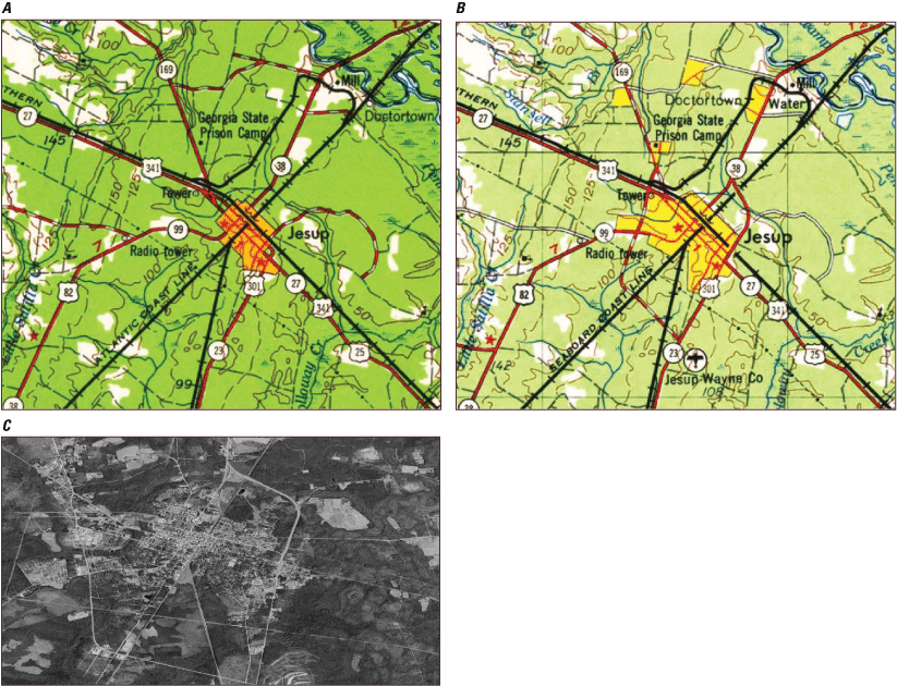
Images of Jesup, Georgia (Ga.), from (A) the 1961 Brunswick, Ga., 1:250,000-scale U.S. Geological Survey (USGS) topographic map (USGS, 1961) top left, (B) a 1978 version (USGS, 1978), top right, and (C) a Hexagon image, December 12, 1974, lower left (USGS, 2023b). Updates to the 1978 version include the addition of the Jesup Wayne County Airport, expanded urban areas, and new roads.
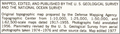
Image of a portion of the map collar from the 1978 Brunswick, Georgia (figure 58), U.S. Geological Survey (USGS) 1:250,000-scale topographic map (USGS, 1978) indicating “other source data” were used to compile the planimetry.
The USGS would also come to rely on Corona and Hexagon images as a source for “photograph revision” to update its 1:24,000-scale topographic maps (fig. 60). The USGS defines photograph revision as “the process of updating maps, from aerial photographs and other available sources to reflect planimetric changes that have occurred since the date of the latest published maps. The revised data are not field checked and are printed in purple” (USGS, 1980). Before they made revisions, USGS cartographers had to determine which topographic maps needed to be revised. The cartographers devised a method for projecting the satellite image onto a published map to determine the quantity of change and used specific criteria to decide whether the map would require revision. If no revision was needed, the USGS reprinted the map with a note explaining “No Revision Required, Inspected 19__” (USGS, 1980). In time, the USGS would rely on 40,000 Corona images to inspect 1:24,000-scale topographic maps for revision (Day and others, 1998, p. 213–214). As before, the use of satellite images from the IC and DOD is obscured through use of the phrase “and other available sources” to protect national security. Through FY 1972, 259 revised maps were produced at the SMC, meaning Corona data were the likely source (White House, 1973, p. 74).
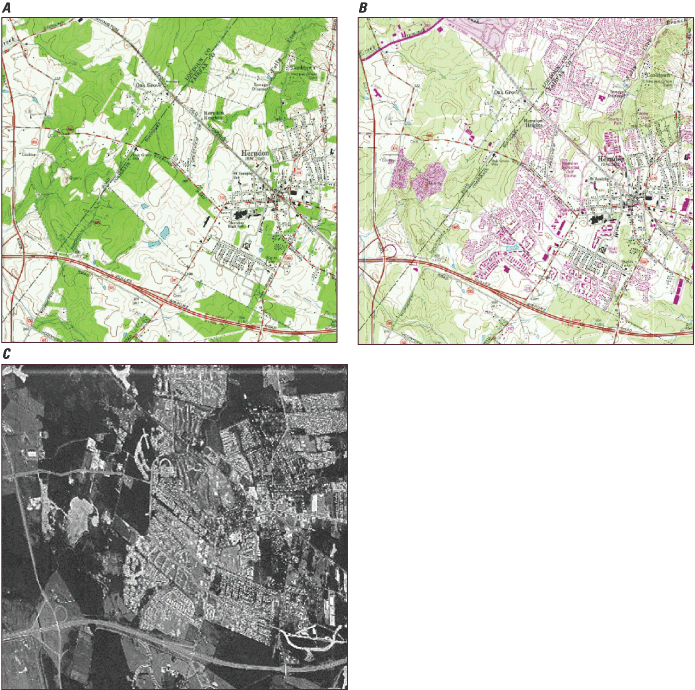
Images of Herndon, Virginia, and vicinity from (A) 1:24,000-scale U.S. Geological Survey (USGS) topographic map (USGS, 1966a), (B) an updated version of the map (USGS, 1966b), and (C) a Hexagon image from Mission 1217, September 5, 1982, likely used in the map update (USGS, 2023e).
In the 1970’s, in addition to topographic maps, the USGS developed the Land Use Data Analysis (LUDA) Program. Turner, in his report to Congress, mentions the production of “detailed land use maps” by the USGS (CIA, 1977a). The LUDA program compiled information from “advanced technology at the SMC of the U.S. Geological Survey, high altitude NASA photographs, aerial photographs acquired for the USGS Topographic Division’s mapping program and LANDSAT data in complementary ways” (Anderson and Witmer, 1975). Certainly, the term “advanced technology at the Special Mapping Center” refers to Corona and Hexagon imagery. In addition, the “high altitude NASA photographs” were acquired by a U–2 plane on loan to NASA (Mitchell and others, 1977, p. 2). In a 1974 memorandum on “Civil Requirements for Satellite Imagery” signed by the Chief of the Forest Service, National Oceanic and Atmospheric Administration [NOAA] Administrator, Chief of the Engineers for the USACE, and the Director of USGS for the COMIREX Chairman transmitting their joint requirements, the USGS requests satellite data to support the LUDA Program (CIA, 1975).
The goal of the USGS in compiling LUDA program data was to produce nationally consistent land-use and land-cover (LULC) maps for the conterminous United States and Hawai’i using the 1:250,000-scale topographic maps as the base. Where there were existing topographic maps at the 1:100,000 scale, those maps were used as the base map. Manual processes delineated polygons of land use and land cover from the above-mentioned data sources using a two-level hierarchical classification system (Anderson and others, 1976). Corona was used specifically at the beginning of the program because it fit the scale of compilation (K.E. Anderson, USGS, retired, written commun., 2023). Later, Hexagon was used as the image source. Because of cloud cover in Alaska, U–2 planes would be on standby to collect aerial photography on cloud-free days as the image source (K. Irby, USGS, retired, written commun., 2023). The USGS published LUDA Program maps at 1:250,000 (fig. 61) and 1:100,000 scales for the conterminous United States, Hawai’i, and one quadrangle in Alaska. The map shown in figure 61 states that the “Land use and land cover information compiled from source information dated 1972.” The vagueness of only stating “source information” rather than the more specific “aerial photography” is consistent with other USGS map products compiled or revised from Corona and Hexagon images or U–2 photographs. Corona Mission 1116 on April 25, 1972 (table 1), or Hexagon Mission 1203 on July 23, 1972 (table 2), are the likely source for the LUDA map shown in figure 61.
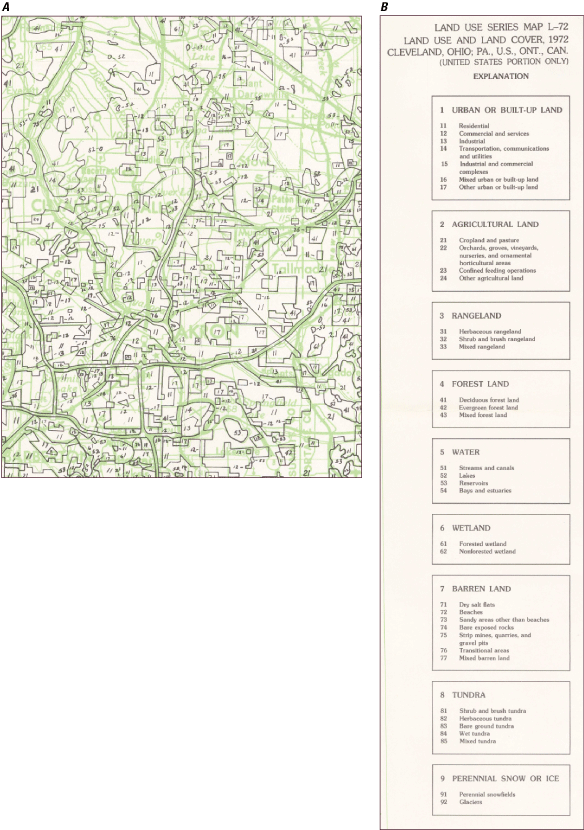
Images from (A) a portion of a map of the Cleveland, Ohio and Pennsylvania, United States; and Ontario, Canada, 1:250,000-scale Land Use and Land Cover Map, 1972, in which a section is showing Akron, Ohio, and areas north. (B) Portion of the U.S. Geological Survey (USGS) map collar with an explanation of the land-use land-cover codes (USGS, 1972).
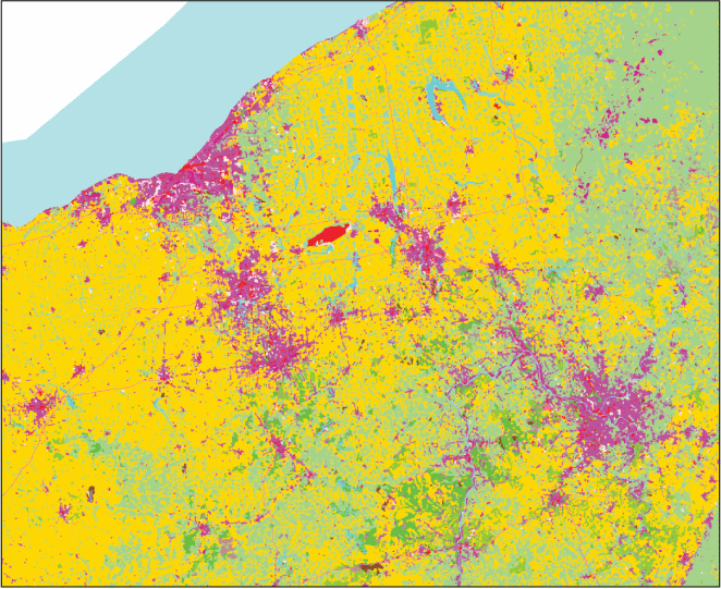
Images of (A) mapped Geographic Information Retrieval and Analysis System data showing northeastern Ohio and western Pennsylvania. Five data classes are represented: purple and red areas are urban/built-up (Cleveland, Akron, Canton, and Youngstown, Ohio, and Pittsburgh, Pennsylvania, are larger urban areas); yellow is agricultural, light green is forest, and light blue is open water (Price and others, 2007).
The USGS converted the paper LUDA maps into the Geographic Information Retrieval and Analysis System (GIRAS) for handling land-use and land-cover data (fig. 62). GIRAS was designed to “accept digitizer input, provide comprehensive editing facilities, produce cartographic and statistical output, permit retrieval and analysis of data, and exercise data base [sic] management tasks” (Mitchell and others, 1977, p. 1).
Several documents reference the USGS mapping Antarctica. The first was to the ARGO Steering Committee in 1968, in which the USGS stated that restrictions were placed allowing no greater detail in the maps than a scale of 1:3,000,000 (White House, 1968d). In a report to Congress on civil applications of classified satellite imagery, CIA Director Turner also referenced Antarctic mapping (CIA, 1977a). Cloud (2002) refers to an Antarctic mosaic created by Autometric, Inc., at the direction of the ARGO Steering Committee. It is unknown which maps were compiled or revised using classified imagery. In 1977, the USGS published a list of series maps of Antarctica it had published and distributed:
-
• 1:250,000-scale, Topographic Reconnaissance Maps,
-
• 1:500,000-scale Topographic Shaded Relief Maps,
-
• 1:250,000-scale Geologic Reconnaissance Maps,
-
• 1:500,000-scale Satellite Image Maps (from Landsat),
-
• 1:500,000-scale Sketch Maps,
-
• 1:1,000,000-scale Topographic Maps,
-
• 1:1,000,000-scale Satellite Image Maps (from Landsat), and
-
• 1:2,188,800-scale Reconnaissance Sketch and Topographic Map.
The 1:500,000-scale Sketch Maps might have been compiled from classified sources, as the description explains that “This is an interim series compiled from the best source data and control available at the time of compilation” (USGS, 1977). The expression “best source data” might indicate that classified images were used, but this is unverified.
The USGS would continue to use classified images to revise its topographic maps and compile thematic maps for another 20 years, eventually building SCIFs at their Rolla, Missouri; Lakewood, Colorado; Sioux Falls, South Dakota; and Menlo Park, California, offices. Eventually, the USGS moved away from map compilation and revision using classified images and relied on unclassified sources maintained or approved by the USGS (Davis and others, 2018, p. 8).
Intelligence Community Influence on the Origins of Landsat
Since the launch of the Landsat 1 satellite (fig. 63) in 1972, the Landsat Program has continually monitored the Earth’s land surface, supporting applications such as crop health and production, tracking water use, documenting urban growth, mapping wildfires and other natural disasters, monitoring the wellbeing of forests, assessing the effects of industrialization, and informing efforts to reduce hunger globally. Landsat 1 was the country’s first civilian land remote-sensing satellite, and since then, the USGS has been responsible for providing worldwide access to Landsat data. Today, the USGS and NASA partner on the Landsat Program through the joint Sustainable Land Imaging Program (USGS, 2020).
Corona was the first land remote sensing satellite and, as the Project ARGO demonstrated, capable of applications beyond military intelligence gathering. With Corona imagery under study to be used by civil agencies and Gemini photography at 15- to 20-ft resolutions, Federal civil leaders, particularly in NASA, the USGS, and the Department of Agriculture, began to make a strong case for a civil remote-sensing satellite in Earth’s orbit.
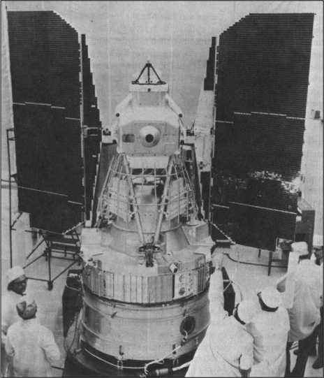
Photograph of the Landsat 1 satellite; appears courtesy of the National Aeronautics and Space Administration.
The IC and Corona played an indirect role in the development of Landsat. The greatest contribution made by the military and the IC to Landsat, according to Mack (1990, p. 37), is the “community of interested and knowledgeable scientists and engineers.” This community comprised military officers, contractors building satellites, Federal civil agency employees granted access to classified imagery, and academic researchers. Scientists with security clearances participating in Project ARGO saw the benefits that satellite imagery could provide in achieving their agencies’ missions. The military’s experience with aerial reconnaissance showed the benefits of collecting intelligence from space.
To expand aerial and satellite sensors beyond traditional aerial photography, the DOD contracted with university laboratories for basic sensor research. One university contractor, the Infrared Laboratory of the Institute of Science and Technology (IST) at the University of Michigan—renamed the “Environmental Research Institute of Michigan” in 1972—played a leading role. As detailed earlier in this report, the early 1960s was a period in which the IST collaborated with the USGS and the military in analyzing infrared imagery of the Kīlauea volcano, building upon the experience and knowledge gained by their work with aerial imagery collected by the military.
In 1946, the military funded work at the Institute that led to the development of defenses against ballistic missiles. When that work was completed, the military funded the Institute in 1954 to investigate the reconnaissance and surveillance of battlefields. The research subsequently led to the development of an aircraft-based scanner system that could observe both visible and infrared wavelengths, essentially a rudimentary multispectral scanner (MSS). The DOD and NASA funded further research by the Institute and a cooperating group at the Hughes Aircraft Company that developed a true MSS. The Hughes Aircraft Company, under the project leadership of Virginia Norwood, would go on to build the MSS that flew on the first Landsat satellite (Mack, 1990, p. 71–72). The MSS might not have been developed if not for the military-funded work by the IST and the Hughes Aircraft Company (fig. 5).
While first focusing on military applications, the Institute would branch out into remote sensing of the environment and, in February 1962, with funding from the Office of Naval Research, held the first Symposium on Remote Sensing of the Environment in Ann Arbor, Mich. Mack (1990) believes that some speakers at the symposium had access to photographs from reconnaissance satellites. However, this information could not be revealed to the audience, so they extrapolated their military experience and research to present a vision for a civilian Earth-resources satellite (p. 38). This symposium series continues under the leadership of an international executive committee composed of representatives from national space agencies. Most recently, the 39th International Symposium on Remote Sensing of Environment was held from April 18–22, 2022, in Hanoi, Vietnam.
In the mid-1960s, NASA’s role was widely considered as that of building and operating a civil Earth-observation satellite. In 1964, NASA began funding several Federal agencies, including the USGS, to advise them about the potential applications of an Earth-resources satellite in geology, cartography, and hydrology. By 1966, NASA had provided $615,000 to the USGS for the Geographic Applications Program (GAP) (CIA, 1966). The USGS became a strong advocate for an accelerated satellite program (Mack, 1990, p. 56–57). At the same time, the USGS–NASA relationship included USGS scientists training Apollo astronauts. USGS scientist Gene Shoemaker convinced NASA to train the astronauts—who up until that time were experienced military test pilots—on scientific fieldwork, deploying instruments, making observations, and collecting lunar rock and soil samples (Vaughan and others, 2019, p. 308).
USGS Director William T. Pecora (fig. 54) knew of Corona, as he sought approval in October 1966 to reprogram money to build the USGS E–1 building and initiate a program to revise topographic maps using Corona imagery. He had also seen the imagery that Gemini astronauts had taken of the Earth’s surface, was aware of their capacity for topographic mapping, and knew about the NASA-funded work done by USGS scientists, including the Peru photomosaic compiled from Gemini photography. However, he and the scientists were impatient with NASA, whose primary focus was meeting President Kennedy’s Moon-landing goal and not Earth remote sensing. These circumstances led Pecora to convince Secretary of the Interior Steward Udall to support and announce, on September 21, 1966, plans to develop an Earth Resources Observations Satellite. Without Congressional authorization or the financial resources to build such a satellite, the announcement was considered as a political move to push NASA into initiating the development of a civilian satellite. The announcement generated wide interest among the press and caused NASA, in 1967, to accelerate the program that ultimately led to the 1972 launch of Landsat 1 (Mack, 1990, p. 60–63).
NASA and the NRO began a longstanding relationship in the early 1960s that contributed to Landsat’s development. Mitchell (2012) explains that NASA enjoyed access to NRO technological information, and the NRO received scientific work relative to space and basic experimentation (p. 209). While it is likely that the NRO contributed to Landsat’s technological development, the NRO also tried to control and influence the sensor’s spatial resolution, as to shield the space-based Earth observation technologies from the Nation’s adversaries.
This tension began with photography planned by the astronauts as part of the Gemini Program that would have resolutions comparable to or better than photographs produced by Corona. NASA's mission was to make data publicly available, which was counter to the NRO's desire to keep the existence of Corona and the country’s ability to collect high-resolution imagery from Earth’s orbit classified. In 1965, NRO was concerned about photographs that would be taken by Gemini astronauts using handheld telephoto-equipped cameras with resolutions of 15–20 ft that were finer than Corona at the time. The two organizations agreed that NPIC would process and review Gemini’s film for intelligence sensitivities. The new procedure went into effect with the Gemini 6 mission launched in December 1965. In the end, the IC was only concerned about two images the astronauts took: one of an aircraft carrier and the other of bombers at an air base (Mitchell, 2012, p. 27).
The issue went beyond Gemini photography. As Mitchell describes, the NSAM 156 committee’s 1966 report was done because NASA was pushing for an Earth-observing program that the NRO thought was too close to the resolutions and capabilities of Corona. NASA was, in fact, considering an Earth-observing program, and in the summer of 1967, the National Academy of Sciences, at NASA’s request, initiated the study “Useful Applications of Earth-Oriented Satellites” and convened 13 panels to examine various aspects of Earth-observing satellites. A panel explored possible geologic applications for satellites from space and proposed either a film-return camera or television-based system referred to as a “return-beam vidicon.” (Summer Study on Space Applications, 1969, p. 9). Doyle (1973, p. 321) then developed a film-return camera like the one used by the Corona satellites. Ultimately, NASA and the NRO agreed, and the NSAM 156 report concurred that NASA sensors would have no better than a 66-ft resolution (Mitchell, 2012, p. 24–32).
In late 1969 and early 1970, NASA and the NRO discussed a tentative plan to satisfy requirements for an Earth-resources survey satellite by adapting Corona systems and technology. NASA declined to pursue Corona satellites because the OMB would not fund the cost (Mitchell, 2012, p. 41).
Landsat would reciprocate with the IC for their technological help. In 1973, NASA Administrator James Fletcher offered Landsat data to the IC to collect economic intelligence on staple food crops (Mitchell, 2012, p. 209). Until that time, Corona and Gambit were used to monitor crops but were limited by the amount of film, the area that could be covered, and the panchromatic (shades of gray) nature of the film used at the time. Landsat’s advantage was that it collected multispectral imagery that was better attuned to monitoring agriculture. The data were already digital, and it could more readily be analyzed; also, repeat coverage over the same area could better track the growing season and the effects caused by changing weather conditions, such as drought.
By 1981, the CIA’s use of Landsat for agriculture tracking was well-established, and the agency was concerned about the program receiving sufficient funding for its continuation. In a memorandum prepared for the CIA Director in 1981, the CIA described their dependence on Landsat for harvest forecasts in the U.S.S.R. (CIA, 1981). Because of Landsat 1’s multispectral sensors, particularly the infrared bands not available on Corona or Hexagon, IC analysts could track soil moisture reserves and crop vigor (CIA, 1977b). Crop estimates and reservoir-level reports for China were also produced using Landsat images (CIA, 1977c). Mitchell (2012, p. 209) contends that the CIA’s use may have prevented the program’s cancellation. NASA moved up the launch date of Landsat 2 to support IC requirements, presumably to continuously monitor spring agricultural production in the U.S.S.R. (Mitchell, 2012, p. 219). This interagency cooperation serves as another example of a close, mutually beneficial relationship (fig. 7).
The IC’s use of civilian remote sensing data was foreshadowed in 1966. An unknown IC employee (their name was redacted in a declassified memorandum) attended an October 1966 National Academy of Sciences and National Research Council (NRC) meeting convened to advise the USGS’s GAP. In a summation of the meeting written to the COMOR Chairman, which, as described earlier, determined the areas collected by classified overhead-aircraft and satellite sensors, the attendee described NASA’s Earth Resources Surveys Program and the USGS’ GAP—both established to set the groundwork and plan the future Landsat Program—and wrote, “Not to be overlooked, however, are the immeasurable benefits from the results of such surveys and scientific findings to our own military interests, to the economic and cultural planning of industrialized nations, and to the orderly development of emerging, less-developed nations” (CIA, 1966).
Landsat was not the only civilian satellite that the military or the IC influenced. The genesis of today’s weather satellites came from the military (fig. 5). In the late 1950s, the USAF’s Air Weather Service (AWS) was involved in Explorer and Vanguard experiments (Dickens and others, 1973, p. 6). Mack reported that early work on meteorological satellites originated at the U.S. Army Ballistic Missile Agency, which was transferred to NASA in 1960 (Mack, 1990, p. 19–20). The DOD’s Advanced Research Projects Agency (ARPA) started studying the use of satellites to picture the Earth’s weather in 1958 and awarded a contract to the Radio Corporation of America to build what became the Television and Infrared Observation Satellite (TIROS). Eventually, in 1959, ARPA turned the project over to NASA. NASA launched TIROS–1 on April 1, 1960, and it operated until June 29, 1960, after capturing nearly 23,000 images (Dickens and others, 1973, p. 46). The U.S. Army Signal Corps downloaded TIROS data for NASA, and NASA turned the images over to the AWS and the U.S. Weather Bureau for analysis (Dickens and others, 1973, p. 30, 39).
TIROS–1 was a success and the first of a series of metrological satellites that continue today. However, concerns over the continued operation of TIROS and its successors led the military to build and launch the Defense Meteorological Satellite Program (DMSP) in 1962, which was driven by the need to determine cloud-free areas for Corona imagery collection. The data were declassified in 1972, and DMSP data are now available to civilian communities. NOAA operates DMSP satellites on behalf of the USSF (USSF, 2023), another example of close civil and military collaboration (fig. 7).
While the linkage from Corona to Landsat is indirect, it is clear that the military and the IC’s reliance on satellite imagery helped propel the use of satellites for land remote sensing by the civil government sector and build a community of experts in the use of satellite imagery for a broad set of applications. When it came time to launch Landsat 1 in 1972, the USGS and other agencies were effectively using Corona imagery to meet their mission requirements. However, usage was still shrouded in secrecy to protect the Nation’s intelligence-reconnaissance capabilities. Landsat data were not classified and could be shared with a broader community without restrictions.
Civil Access Codified
Initially, Federal civil agencies were using Corona and U–2 imagery under the coordination and oversight of Project ARGO. Later, the ARGO Steering Committee was overseen by the President’s Science Advisor. President Nixon abolished the role of Presidential Science Advisor in 1973, and the ARGO Steering Committee ceased to exist. During this time, coordination and oversight of civil-agency use of military and IC overhead-capabilities no longer existed (Baclawski and Nath, 2002). Until the early 1970s, Federal civil agency access to Corona and Hexagon imagery had not been legally codified. Some in the IC expressed concern over the lack of clear legal guidance. However, White House senior officials were engaged with ARGO and the BOB; the latter was under the Executive Office of the President, which led the mapping study and thus made decisions allowing civil agencies to access classified data. Congress appropriated funds for the USGS to build and operate the E–1 building and conduct the map revision program, but no authorizing language was approved. Clear policy statements were yet to be made, and following the abolishment of the ARGO Steering Committee, no coordination mechanisms existed.
National Security Adviser Henry Kissinger suggested that the DCI establish a civil agency subcommittee under COMIREX to coordinate image requirements. The proposal was reviewed by CIA staff. In a suggested statement to be made by the DCI, the issue of legal authority to collect data over domestic areas was raised, and the drafted statement requests Presidential authority be granted, stating,
“the authority of the President to declare that certain national photographic reconnaissance assets are in service of the civil agencies during periods of their use and support of U.S. civil applications and thus not in service of the foreign intelligence community at those specific times” (CIA, 1973).
In that same packet of correspondence, a draft statement was written for the DCI, which stated, in part:
“The use of national photographic reconnaissance assets, particularly satellites, to assist the civil arms of the U.S. Government, raise concern questions of propriety. These assets have been developed and used as foreign intelligence capabilities and the National Security Act of 1947 forbids the Central Intelligence Agency from engaging in certain domestic activities.”
In a December 1973 memorandum to the DCI with the subject “Civil Use of Classified Reconnaissance System, Technologies, & Products,” a CIA staff member wrote, “I recommend that you task OLC [Office of Legal Counsel] to gain acceptance of this concept and implementation with the appropriate subcommittees of Congress” (CIA, 1973). It is unknown if the committee was ever established.
Civil Applications Committee
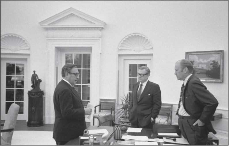
Photograph of President Gerald Ford (right) conversing with Vice President Nelson Rockefeller (center) and Secretary of State and National Security Advisor Henry Kissinger (left) in the Oval Office of the White House in 1975. Photograph appears courtesy of the National Archives and Records Administration.
On December 22, 1974, the New York Times published an investigation detailing the domestic activities undertaken by the CIA, activities which the authors contended were illegal (Hersch, 1974). In response, on January 4, 1975, President Gerald Ford (fig. 64) established the “United States President's Commission on CIA Activities within the United States” to investigate the allegations and placed his Vice President, Nelson Rockefeller, as commission chair. Informally, the commission is known as the “Rockefeller Commission.” Part IV, Chapter 16, pages 230–231 of the commission’s final report (U.S. Commission on CIA Activities Within the United States, 1975) acknowledges that the CIA was sharing “aerial intelligence photography”—likely Corona, Hexagon, and U–2 photographs—with civilian agencies:
“The photographs of the United States actually turned over to civilian agencies were taken primarily for military mapping purposes. Since that time, aerial photography systems have been used for such diverse civilian projects as mapping, assessing natural disasters such as hurricane and tornado damage and the Santa Barbara, California oil spill, conducting route surveys for the Alaska pipeline, conducting national forest inventories, determining the extent of snow cover in the Sierras to facilitate the forecast of runoff and detecting crop blight in the plain states. Limited equipment testing and performance evaluation is also conducted using photographs taken of areas within the United States.” (U.S. Commission on CIA Activities Within the United States, 1975, p. 230)
As part of its conclusion to this chapter, the committee wrote:
“The Commission can find no impropriety in permitting civilian use of aerial photography systems. The economy of operating a single aerial photography program dictates the use of these photographs for appropriate civilian purposes.” (U.S. Commission on CIA Activities Within the United States, 1975, p. 231)
A footnote to this conclusion addressed the use of these data for law enforcement; it states:
“It is arguable that at least one present use of aerial photography is law enforcement in nature and outside the scope of proper CIA activities. This use involves photography with infrared sensors to detect areas of high concentrations of industrial pollutants in the air and in various bodies of water. Data obtained from this activity could conceivably be used as the basis for a criminal action brought under environmental legislation. The Commission believes, however, that the legislators, when they prohibited the CIA from engaging in law enforcement activities in their 1947 enactment of the National Security Act, could not have contemplated the system presently in use. It should be noted that the CIA did turn down a request from the Alcohol and Tobacco Tax Unit of the Treasury Department to help locate moonshine stills in the North Carolina mountains using infrared photography, on the ground that such activity was law enforcement in nature.” (U.S. Commission on CIA Activities Within the United States, 1975, p. 231)
The Commission report made one of its recommendations the establishment of an oversight and coordination committee:
“Recommendation (29): A civilian agency committee should be reestablished to oversee the civilian uses of aerial intelligence photography in order to avoid any concerns over the improper domestic use of a CIA-developed system” (U.S. Commission on CIA Activities Within the United States, 1975, p. 231).
President Ford, in accepting the recommendations of the Rockefeller Commission, directed, in an August 16, 1975, memorandum, that Recommendation 29, among several others, be implemented and instructed the preparation of a draft directive establishing an interagency committee to oversee the domestic uses of aerial intelligence photography (White House, 1975a).
In an October 3, 1975, memorandum (White House, 1975b) prepared in response to the August 13 memorandum from President Ford, Henry A. Kissinger (fig. 64), President’s National Security Advisor, William E. Colby, DCI, and James T. Lynn, Director, OMB, directed the Secretary of the Interior to form the “Committee for Civil Applications of Classified Overhead Photography of the United States.” The memo formed the first charter of what today is called the Civil Applications Committee (CAC). The Committee was to take the following actions:
-
• “Receive, evaluate, consolidate, standardize, establish priorities and transmit to the Director of Central Intelligence all requests for such photography from domestic civilian agencies;
-
• Facilitate civilian agencies’ use of classified systems and coordinate the incorporation of photography, derived data, and technology and performance of domestic civilian functions;
-
• Supply information to civilian agencies so that they may knowledgeably formulate requests and reach compromise between request and capabilities;
-
• Act as an interface between civilian agencies and intelligence collectors, recognizing that the Director of Central Intelligence will not be involved in judgments concerning civil agency needs or priorities and that collection for this purpose will remain incidental to foreign intelligence collections;
-
• Overseas civilian agency uses of classified photography in a manner designated to avoid any concerns that domestic photographic coverage is being used improperly” (White House, 1975b).
The memorandum further directed that the committee was to be chaired by a representative from the DOI and “will consist of representatives of the Departments of Agriculture and Commerce, the National Aeronautics and Space Administration, the Corps of Engineers and the Environmental Protection Agency” with additional members added at the discretion of the committee (White House, 1975b). The Acting Secretary of the Interior replied on December 10, 1975, and designated William A Radlinski, the USGS Associate Director, as the committee chair and Roy E. Fordham, Chief, SMC, as the immediate backup (DOI, 1975).
Baclawski and Nath (2002) contend that the “1973 abolition of the position of the president science advisor left no oversight authority for such activities and recommended that an interagency committee of Federal civil agencies be established to oversee such applications.” Baclawski spoke from a unique perspective in that he attended many of the early CAC meetings as a representative of the COMIREX. Clark and Hemphill (2002) suggested the establishment of the CAC was one of the long-term outcomes of the 1969 Santa Barbara Channel oil spill, presumably because the military’s U–2 plane was used to collect aerial imagery (fig. 57) over the domestic areas used to manage the cleanup.
The first meeting of the Committee for Civil Applications of Classified Overhead Photography of the United States took place on January 23, 1976, at the USGS SMC in Reston, Va. William Radlinski chaired the meeting; Roy E. Fordham served as the first executive secretary. Attendees were from the USACE, NASA, NOAA, EPA, USFS, USAF, and COMIREX. At this first meeting, the group discussed operational guidelines, procedures for submitting image requirements, downgrading materials to the “Secret” or unclassified level, and how agencies should be encouraged to use the USGS facility. By the third meeting, on March 23, the name had been shortened to “Civil Application Committee,” and was even further shortened to the acronym “CAC.” This name is still used (Opstal and Rogers, 2022; USGS, 2023a).
The CAC met eight times in 1976, with seven of the meetings held at the USGS E–1 building and one held at the CIA headquarters. The latter was not an official meeting but rather a “dry-run” of briefings given to other Federal agencies to increase awareness of the imagery and its use and the availability of the USGS facility. During its first year, the committee established operational guidelines and agreed to exclude collection requests regarding foreign areas. For this reason, the committee denied USAID’s request for committee membership, as to not appear concerned about foreign data collection. However, the Defense Mapping Agency (DMA), the NRO, and a COMIREX representative were added as observers. The committee also established a Working Group on Requirements to coordinate image collection requests from agencies for approval by the CAC and submittal to the DCI. Outreach to Federal agencies not on the CAC was also planned, culminating with a Secret-level briefing held in October 1976 at CIA headquarters with 167 people in attendance.
Collection requirements were consolidated by the Working Group on Requirements, reviewed at the April 12 CAC meeting, and approved at the June 4 meeting. A summation of the justifications follows:
-
• USACE: environmental analysis of a dam site and feasibility study on remote sensing for environmental studies;
-
• EPA: point and nonpoint survey for monitoring pollution sources; impact of land-use on water quality; strip mine inventory; and power plant monitoring;
-
• USFS: damage assessment due to disease and invasive beetles, National Forest map revision; study of soils, watershed potential, vegetation, and forest classification;
-
• National Ocean Service: Nautical Chart Revision, Aeronautical Chart Revision;
-
• Soil Conservation Service: tree patterns, land-use patterns;
-
• USGS: planimetric revisions of 1:24,000-, 1:100,000-, and 1:250,000-scale topographic maps and delineation of land-use maps (USGS, 2023a).
Since the CAC established its initial policies and procedures in its first year of operation, the pace of meetings decreased in the following years. The CAC met three times each year in 1977 and 1978 and once in 1979 (USGS, 2023a).
In 1977, William Radlinski continued as the chair, and Roy Fordham continued as the executive secretary. A new online procedure—the COMIREX Automated Management System (CAMS)—was described to submit agency requests for imagery; the USGS requested a CAMS terminal be installed in the E–1 building. The CAC discussed their individual agency’s input to a National Space Policy that the Assistant to the President for National Security Affairs was leading (refer to the “National Space Policy” section in this report). Fordham discussed requirements for Hexagon Mission 1213, which was launched later in the year (table 2). Members were also apprised of updated security instructions, which required 5-year updates of security clearances.
The Energy Research and Development Administration (ERDA) requested and was granted membership at the May 10, 1977, meeting. ERDA membership transitioned to the Department of Energy upon that agency’s establishment later in 1977. Also, during the May meeting, members were updated on the National Space Policy, and members were asked to submit “Proper Use” statements for committee approval. The committee at the November 9, 1976, meeting determined Proper Use statements are—
“defined as the utilization of imagery and information derived from classified overhead imagery systems that is in support of Congressionally approved programs of the user agency, and that is not in violation of applicable laws, including the statutory authority of the user agency, nor inconsistent with the constitutional and other legal rights of United States persons.” (USGS, 2023a, p. 73)
Other topics discussed were security guidelines, the use of aerial photography from the SR–71 and U–2 military aircraft, and a legal briefing intended to provide guidelines on the use of classified imagery. The SR–71 was a high-altitude reconnaissance aircraft flown from the mid-1960s to the late 1990s. Finally, the DMA requested use of equipment in the E–1 building. The committee tabled that topic, as they were concerned with using a civil facility for intelligence purposes. No further mention of this topic appeared in subsequent CAC meeting minutes.
During the November 1977 meeting, members were briefed on legal guidelines for domestic tasking, heard an update on the National Space Policy review, discussed their requirements for SR–71 and U–2 aerial photography, learned that agencies’ request for image collection would fall short of the 400,000 nmi2 requested, and received an update on the security manual. The COMIREX member noted that a draft report on nonmilitary uses of classified imagery was sent to the new DCI (USGS, 2023a, p. 93). Later, the report was sent to Congress (CIA, 1977a).
The CAC met three times in 1978 on April 13, June 20, and September 26. Radlinski and Fordham continued in their respective roles as chair and executive secretary. At the April meeting, the CAC approved a request for Hexagon mapping camera collection over Antarctica, which COMIREX later approved. Members learned at the June meeting that the President’s National Space Policy was approved on May 11 (refer to “National Space Policy” section in this report). The Department of Agriculture member discussed concerns that imagery had not been collected and requested that an earlier determination in the growing season would have helped the agency develop other plans. At the September meeting, the chairman invited CAC members to attend a briefing planned for December at the E–1 building for Senator Adlai Stevenson about classified activities.
The chair announced that the DCI had authorized the USGS to produce unclassified photomaps, also known as an orthophoto quadrangle. The USGS had produced 22,000 orthophoto quadrangles from unclassified aerial photography and would now augment production with Hexagon imagery. Thompson (1987, p. 135) defines an orthophoto quadrangle as “a monocolor orthophotographic map presented in standard quadrangle format and related to the standard horizontal reference system. It has no contours and has little or no cartographic treatment.” Members also learned that the DCI had approved USGS’s request to construct a SCIF at their Rolla, Mo., mapping center (USGS, 2023a, p. 124, 134).
Only one CAC meeting was held in 1979, on October 25, over a year from the prior meeting. The CAC approved requirements for Hexagon Mission 1216 (table 2) and reviewed the accomplishments for Mission 1215 (which members thought was low) with 138,000 nmi2 collected to meet Federal civil agency requirements. The COMIREX representative reviewed policy issues, and Fordham said the Rolla office was in production (USGS, 2023a, p. 141).

Image showing the official seal of the Civil Applications Committee. Image appears courtesy of the U.S. Geological Survey.
The CAC continues to meet and “facilitates the appropriate civil uses of overhead remote sensing technologies and data collected by military and intelligence capabilities, including from commercial sources” (Opstal and Rogers, 2022) and considers itself working at the “triple junction” (fig. 1) with Federal civil agencies as the third circle. Figure 65 depicts the CAC seal in use today, which depicts a satellite in Earth’s orbit with landscape symbols representing civil agency missions.
National Space Policy
Landsat and the increasing interest among Federal civil agencies in data and information about the Earth from orbit, along with the growing role of space-based reconnaissance by the military and intelligence communities, and technology converging such that civil satellite capabilities could approach those of classified systems brought to the forefront the conflicts and potential overlap between NASA and the NRO. In addition, the Strategic Arms Limitation Treaty signed by the United States and the U.S.S.R. in 1972 alluded to the use of satellite reconnaissance—termed “National Technical Means of Verification”—to monitor treaty compliance, opened the question of acknowledging and declassifying America’s national reconnaissance capabilities. The term was shortened to National Technical Means, or NTM, and would continue to be used as an unclassified term to indicate classified IC or DOD remote sensing systems. To this end, in 1975, the DOD, NRO, and NASA attempted several governing structures to address policy issues, such as the spatial resolution of civil satellites, declassification of the fact of reconnaissance from space, responsibilities of NASA and NRO, coordination between the two agencies, and use by civil agencies. National Security Advisor Henry Kissinger brought it to the attention of President Ford, who directed the establishment of the Space Policy Committee.
In its November 1976 report to the President, the committee agreed to six recommendations, including the limited expansion of imagery use by civil agencies. An unresolved issue was the declassification of the Nation’s intelligence reconnaissance capabilities. Having lost the Presidential election to Jimmy Carter (fig. 66), Ford deferred this and other space-related policy questions to the incoming administration. In March 1977, President Carter directed a comprehensive review of U.S. space policy with a focus on the relationships among the civilian and national security space programs. Each government committee, including the CAC, was invited to provide comments and make suggestions on draft versions of the policy. The review resulted in the drafting of a National Space Policy document, which the President approved and signed on May 11, 1978, as Presidential Directive/National Security Council 37 (Mitchell, 2012, p. 54–60). Of note to civil agencies is that the policy continued their use of military systems:
“Selected space related products and technology shall be made available to civil agencies within appropriate security constraints. The Intelligence Community may provide radio frequency (RF) mapping and surveys for the civil community under appropriate security controls.”
The policy further stated—
“Expanded civil use of intelligence space data and technology within appropriate security constraints is encouraged.” (White House, 1978).
With President Ford’s establishment of the CAC, President Carter’s National Space Policy, and annual Congressional appropriations to the USGS to operate its classified mapping program, Federal civil agencies’ equities in the access to and use of DOD and IC remote sensing systems and data to support their statutory missions became well-established in national policy.
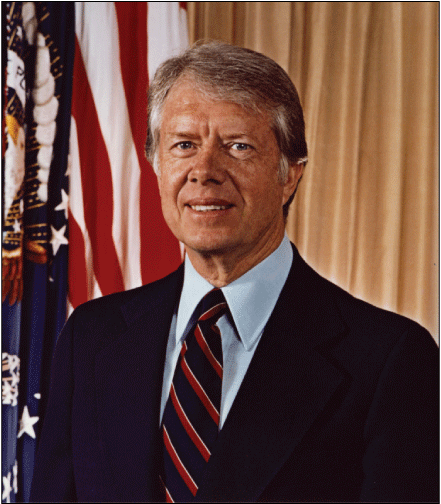
Photograph of President Jimmy Carter; appears courtesy of the Jimmy Carter Presidential Library.
Summary
At the invitation of the American Society on Photogrammetry and Remote Sensing, Charles Andregg, the former Deputy Director of the DMA, wrote on the military–USGS mapping cooperation on the USGS’s 100th anniversary in 1979 (Andregg, 1979). Andregg concluded that “this [military–USGS cooperation] has been a continuing and very important relationship since our military mapping and charting community is at once an ancestor, a collaborator, and a major customer of the Geological Survey.” His comments parallel and highlight the conclusions of this report on the development of the close, collaborative relationship between Federal civil agencies, particularly the USGS, and the IC and DOD, as represented in figure 1.
Andregg writes about how the need for topographic maps was driven by military requirements and the need for explorers to document their findings. He discusses the role of General George Washington’s establishment of a military mapping unit to support Revolutionary War efforts, the connections between civilian mapping and exploration efforts following the war, and the military men or former military men who led those efforts, mentioning names listed earlier in this report: Meriwether Lewis, William Clark, John Fremont, Gouverneur Warren, William Emory, and Zebulon Pike. With the establishment by the U.S. Army Corps of Topographic Engineers (today’s USACE) in 1838, officers and enlisted personnel were trained to conduct mapping efforts, and this training culminated in the Wheeler Survey of the Western United States.
Once the USGS was established, many of the Army-trained mapping and surveying personnel from the “Four Great Surveys of the West” transitioned to the USGS and continued its topographic mapping efforts. Eventually, the Army turned to the USGS for maps of domestic areas. As Andregg confirms, the collaboration continued during World War I, with the technological development of photogrammetry, the use of aerial photography to compile topographic maps, and the joint mapping work during World War II. Andregg leaves off that the DMA and USGS are “formalizing the exchange of technical personnel, and of the coordination of acquisition and systems.” In 1979, the USGS’s use of classified remote-sensing images to revise topographic maps was still classified; as a result, that topic is not covered in his article nor in any other unclassified publication before President Clinton’s declassification of Corona in 1995.
In 1981, the National Academy of Sciences reviewed the current relationship between the defense and civilian mapping agencies. Before the study, in 1972, the DOD established the DMA by consolidating 80 percent of the DOD’s MC&G staff into a single agency to serve the national security community’s needs for maps (NRC, 1981, p. 47). For military mapping needs in domestic areas, DMA relies on civil agencies such as the USGS as Andregg confirmed in his remarks made in 1979. As the NAS study reported, the DMA relied on advanced technology to map inaccessible foreign areas and shared that advanced technology with civil agencies. Terms such as “advanced technology” were often used to describe classified remote sensing capabilities, as with Corona and Hexagon satellite images, the fact of which remained classified. The USGS produced 1:24,000-, 1:50,000-, and 1:250,000-scale topographic and special maps to meet DMA’s needs. The two organizations also worked on the maintenance of joint civilian-military digital terrain data for the United States and the standardization of data file formats and entered formal agreements for cooperation in research and development, along with the procurement of production systems (NRC, 1981).
Today’s close, collaborative relationship in the mapping and remote sensing sciences between the DOD, IC, and Federal civil agencies (fig. 1), particularly the USGS, developed over time. This collaboration benefited both the DOD–IC and the Federal civil sector. The USGS mapping and remote-sensing functions realized great advantages in their relationship with the DOD and IC, and in return, the DOD and IC also realized benefits.
References Cited
Anderson, J.R. and Witmer, R.E., 1975, The national land use data program of the U.S. Geological Survey in Proceedings of the NASA Earth Resources Survey Symposium, Houston, Texas, June 1975—First Comprehensive Symposium on the Practical Application of Earth Resources Survey Data: Houston, Tex., Lyndon B. Johnson Space Center, v. 1–C, [June 1, 1975], 7 p., accessed November 18, 2023 at https://ntrs.nasa.gov/api/citations/19760010471/downloads/19760010471.pdf.
Anderson, J.R., Hardy, E.E., Roach, J.T., and Witmer, R.E., 1976, A land use and land cover classification system for use with remote sensor data: [U.S.] Geological Survey Professional Paper 964, 28 p., accessed November 25, 2023, at https://doi.org/10.3133/pp964.
Andregg, C.H., 1979, Military-USGS Mapping Cooperation: Photogrammetric Engineering and Remote Sensing, v. 45, no. 12, p. 1621–1624, accessed December 4, 2023, at https://www.asprs.org/wp-content/uploads/pers/1979journal/dec/1979_dec_1621-1624.pdf.
Baclawski, J.A. and Nath, T.B., 2002, Civil Applications Committee’s role in national reconnaissance: National Reconnaissance Office, Center for the Study of National Reconnaissance Bulletin, combined 2002 issue, p. 13, accessed August 30, 2023, at https://www.governmentattic.org/docs/NRO_CSNR_Bulletin_Comb2002Issue.pdf.
Bagley, J.W., 1917, The use of the panoramic camera in topographic surveying with notes on the application of photogrammetry to aerial surveys: U.S. Geological Survey Bulletin 657, 88 p., accessed January 4, 2023, at https://doi.org/10.3133/b657.
Baker, D. J. and Zall, L., 2020, The MEDEA Program—Opening a window into new earth science data: Oceanography, v. 33, no.1, p. 20–31, accessed March 2, 2023 at https://doi.org/10.5670/oceanog.2020.104.
Beydler, H., [undated], Soldier of the Two World Wars—Mapmaker, Daniel O’Madigan Kennedy Celebrates His First 100 Years: U.S. Geological Survey web page, accessed January 16, 2023, at https://www.usgs.gov/human-capital/soldier-two-world-wars.
Brugioni, D.A., 1970, The serendipity effect: Central Intelligence Agency, Studies in Intelligence, v. 14, no. 1, p. 43–76, accessed March 3, 2023, at https://www.cia.gov/readingroom/docs/CIA-RDP78T03194A000300010009-3.pdf.
Campbell, J.B., 2008, Origins of aerial photographic interpretation, U.S. Army, 1916 to 1918: Photogrammetric Engineering & Remote Sensing, v. 74, no. 1, p. 77–93, accessed January 4, 2023, at https://doi.org/10.14358/PERS.74.1.77.
Casana, J., Goodman, D.D., Ferwerda, C., 2023, A wall or a road? A remote sensing-based investigation of fortifications on Rome's eastern frontier: Antiquity, v. 97, no. 396, p. 1–18, accessed November 25, 2023, at https://doi.org/10.15184/aqy.2023.153.
Central Intelligence Agency [CIA], 1962, [Correspondence between the U.S. Geological Survey and the U.S. Army Corp of Engineers from June to December 1962]: CIA document release CIA–RDP78B04747A000100030009–9, approved for release August 22, 2000, [12 p.], accessed January 31, 2023, at https://www.cia.gov/readingroom/docs/CIA-RDP78B04747A000100030009-9.pdf.
Central Intelligence Agency [CIA], 1963a, Staff Study—Multi-sensor reconnaissance survey of east rift zome [sic] of Volcano Kilanea, Hawaii: CIA release document CIA–RDP78B04747A000100030005–3, approved for release August 22, 2000, [8 p.], accessed January 24, 2023, at https://www.cia.gov/readingroom/docs/CIA-RDP78B04747A000100030005-3.pdf.
Central Intelligence Agency [CIA], 1963b, Institute of Science and Technology, The University of Michigan—News release, January 24, 1963: CIA document release CIA–RDP78B04747A000100030001–7, approved for release August 22, 2000, [3 p.], accessed February 23, 2023, at https://www.cia.gov/readingroom/docs/CIA-RDP78B04747A000100030001-7.pdf.
Central Intelligence Agency [CIA], 1964, [Routing slip, memorandum, and article titled “Infrared Surveys of Hawaiian Volcanos,” declassified in part]: CIA document release CIA–RDP78B05167A000800050001–1, sanitized copy approved for release January 15, 2014, [12 p.], accessed February 23, 2023, at https://www.cia.gov/readingroom/docs/CIA-RDP78B05167A000800050001-1.pdf.
Central Intelligence Agency [CIA], 1966, [Routing and memorandum with attachments—Briefing note on the potential use of remote sensors for studying and recording data on the Earth’s resources—declassified in part]: CIA document release CIA–RDP80T01137A000600010011–2, sanitized copy approved for release April 26, 2012, [12 p.], accessed September 9, 2023, at https://www.cia.gov/readingroom/docs/CIA-RDP80T01137A000600010011-2.pdf.
Central Intelligence Agency [CIA], 1967, Journal—Office of Legislative Affairs: CIA document release CIA–RDP69B00369R000100180185–2, approved for release March 11, 2004, 1 p., accessed January 31, 2023, at https://www.cia.gov/readingroom/docs/CIA-RDP69B00369R000100180185-2.pdf.
Central Intelligence Agency [CIA], 1968a, Memorandum for the United States Intelligence Board—Plans for use of TALENT/KEYHOLE data by the United States Geological Survey, March 28, 1968: CIA document release C05106760, approved for release May 2, 2019, [4 p.], accessed March 17, 2023 at https://ia904507.us.archive.org/0/items/nro-fta-scrape/Plans%20for%20Use%20of%20TALENT%20KEYHOLE%20Data%20by%20the%20United%20States%20Geological%20Su rvey.pdf.
Central Intelligence Agency [CIA], 1968b, COMIREX Mapping, Charting and Geodesy Working Group, minutes of meeting held in room 5B2830, 1330–1600, 19 February 1968: CIA document release CIA–RDP79B01709A000500010047–6, approved for release October 10, 2003, [7 p.], accessed March 17, 2023 at https://www.cia.gov/readingroom/docs/CIA-RDP79B01709A000500010047-6.pdf.
Central Intelligence Agency [CIA], 1969a, Committee on Imagery Requirements and Exploitation—COMIREX–M–63 [meeting minutes, 13 February 1969: CIA document release CIA–RDP79B01709A000800020002–1, approved for release April 17, 2003, [22 p.], accessed March 17, 2013 at https://www.cia.gov/readingroom/docs/CIA-RDP79B01709A000800020002-1.pdf.
Central Intelligence Agency [CIA], 1969b, Memorandum for [Committee on Imagery Requirements and Exploitation, Mapping, Charting and Geodesy Working Group], Notes on the MC&G Working Group meeting of 22 April 1969: CIA document release CIA–RDP79B01709A000400030059–2, approved for release February 17, 2005, [9 p.], accessed March 19, 2023 at https://www.cia.gov/readingroom/docs/CIA-RDP79B01709A000400030059-2.pdf.
Central Intelligence Agency [CIA] 1969c, Memorandum for the Record—Steering Committee/ARGO Meeting of 9 December 1969: CIA document release CIA–RDP80T01137A0002000060001–2, [6 p.], accessed March 11, 2023, at https://www.cia.gov/readingroom/docs/CIA-RDP80T01137A000200060001-2.pdf.
Central Intelligence Agency [CIA], 1971, Memorandum for Chairman, COMIREX—Satellite photography of the U.S. for United States Geological Survey mapping activities: CIA document release CIA–RDP79B01709A000400030004–2, approved for release July 7, 2004, [4 p.], accessed March 19, 2023, at https://www.cia.gov/readingroom/docs/CIA-RDP79B01709A000400030004-2.pdf.
Central Intelligence Agency [CIA], 1973, [Various correspondence concerning draft memorandum civil use of classified reconnaissance systems, technologies and products]: CIA document release CIA–RDP76B00734R000100210002–6, approved for release March 15, 2006, [24 p.], accessed March 14, 2023, at https://www.cia.gov/readingroom/docs/CIA-RDP76B00734R000100210002-6.pdf.
Central Intelligence Agency [CIA], 1975, [Various correspondence to and from COMIREX on civil uses of satellite technology—declassified in part]: CIA document release CIA–RDP80M01133A000500100030–0, sanitized copy approved for release January 17, 2007, [38 p.], accessed November 15, 2023, at https://www.cia.gov/readingroom/docs/CIA-RDP80M01133A000500100030-0.pdf.
Central Intelligence Agency [CIA], 1976, USIB Committee on Imagery Requirements and Exploitation (COMIREX): CIA document release CIA–RDP79B01709A001400020029–4, sanitized copy approved for release August 14, 2012, 1 p., accessed September 9, 2023, at https://www.cia.gov/readingroom/docs/CIA-RDP79B01709A001400020029-4.pdf.
Central Intelligence Agency [CIA], 1977a, Memorandum for the Honorable Daniel K. Inouye, Chairman, Senate Select Committee on Intelligence—Transmitting requested report on nonmilitary uses of intelligence assets, [signed S. Turner]: CIA document release CIA–RDP8300171R001200190001–4, approved for release November 3, 2007, [35 p.], accessed February 23, 2023, at https://www.cia.gov/readingroom/docs/CIA-RDP83M00171R001200190001-4.pdf.
Central Intelligence Agency [CIA], 1977b, USSR—Status of the 1976/77 Winter Grains—Environment Analysis Brief, January 31, 1977: CIA document release CIA–RDP79–01056A000100120001–0, approved for release April 27, 2001, 4 p., accessed November 25, 2023, at https://www.cia.gov/readingroom/docs/CIA-RDP79-01056A000100170001-0.pdf.
Central Intelligence Agency [CIA], 1977c, China Crop Environmental Brief—1977, First Report, June 1977: CIA document release CIA–RDP79–01056A000100010001–7, approved for release April 9, 2001, [12 p.], accessed November 25, 2023, at https://www.cia.gov/readingroom/docs/CIA-RDP79-01056A000100010001-7.pdf.
Central Intelligence Agency [CIA], 1981, Memorandum for Director of Central Intelligence—CCCT Meeting—Landsat issue [redacted], December 15, 1981: CIA document release CIA–RDP84B00049R001700060018–4, approved for release March 20, 2007, [3 p.], accessed August 29, 2023, at https://www.cia.gov/readingroom/docs/CIA-RDP84B00049R001700060018-4.pdf.
Clark, K.C. and Hemphill, J.J., 2002, The Santa Barbara oil spill—A retrospective in Danta, D., ed., [2002], Yearbook of the Association of Pacific Coast Geographers: [Honolulu, Hawaiʻi], University of Hawai'i Press, v. 64, p. 157–162, accessed March 6, 2023, at https://doi.org/10.1353/pcg.2002.0014.
Cloud, J., 2001, Imaging the world in a barrel—Corona and the clandestine convergence of the earth sciences: Social Studies of Science, v. 31, no. 2, p. 231–251, accessed March 10, 2023, at https://doi.org/10.1177/0306312701031002005.
Cloud, J., 2002, American cartographic transformations during the Cold War: Cartography and Geographic Information Science, v. 29, no. 3, p. 261–282, accessed February 15, 2023, at https://doi.org/10.1559/152304002782008422.
Collier, P., 2002, The impact on topographic mapping of developments in land and air survey—1900–1939: Cartography and Geographic Information Science, v. 29, no. 3, p. 155–174, accessed February 15, 2023, at https://doi.org/10.1559/152304002782008440.
Davis, L.R., Fishburn, K.A., Lestinsky, H., Moore, L.R., and Walter, J.L., 2018, US Topo Product Standard (ver. 2.0, February 2019): U.S. Geological Survey Techniques and Methods book 11, chap. B2, 20 p., 3 pls., scales 1:24,000, 1:25,000, and 1:20,000, accessed January 4, 2023, at https://doi.org/10.3133/tm11B2.
Dickens, C.W., Ravenstein, C.A., and Fuller, J.F., ed., 1973, Air Weather Service and meteorological satellites, 1950–1960: Scott Air Force Base, Ill., Air Weather Service, Military Airlift Command, United States Air Force, 164 p., accessed September 23, 2023, at http://www.airweaassn.org/reports/Pages%20from%20Air%20Weather%20Service%20and%20Meteorological%20Satellites,%201950--1960_partA.pdf.
Defense Mapping Agency [DMA], 1982, MC&G—Mapping, charting, geodesy—A brief history of U.S. military mapmaking, and the first decade of the Defense mapping agency: Washington, D.C., Defense Mapping Agency, 41 p., accessed July 4, 2023, at https://catalog.hathitrust.org/Record/002171654.
Desmond, G.B., 2003, Measuring and mapping the topography of the Florida Everglades for ecosystem restoration: U.S. Geological Survey Fact Sheet 021–03, 4 p., accessed February 1, 2023, at https://doi.org/10.3133/fs02103.
Doyle, F.J., 1973, Can satellite photography contribute to topographic mapping?: Journal of Research of the U. S. Geological Survey, v. 1, no. 3, p. 315–325, accessed April 6, 2024, at https://pubs.usgs.gov/journal/1973/vol1issue3/report.pdf.
Evans, R.T. and Frye, H.M., 2009, History of the topographic branch (division): U.S. Geological Survey Circular 1341, 196 p., accessed January 4, 2023, at https://doi.org/10.3133/cir1341.
Fisher, G.B., Slonecker, E.T., Dilles, S.J., Molnia, B.F., and Angeli, K.M., 2023, Using global Fiducials Library high-resolution imagery, commercial satellite imagery, Landsat and Sentinel satellite imagery, and aerial photography to monitor change at East Timbalier Island, Louisiana, 1953–2021: U.S. Geological Survey Scientific Investigations Report 2022–5107, 61 p., accessed November 25, 2023, at https://doi.org/10.3133/sir20225107.
FitzGerald, G., 1951, Surveying and Mapping in Alaska: U.S. Geological Survey Circular 101, 24 p., accessed February 23, 2023, at https://doi.org/10.3133/cir101.
Forti, L., Pelfini, M., Sissakian, V.K., Zerbini, A., 2023, Settling the riverscape of Erbil (Kurdistan region of Iraq)—long-term human overprint on landforms and present-day geomorphological hazard: Anthropocene, v. 44, article 100413, accessed November 25, 2023, at https://doi.org/10.1016/j.ancene.2023.100413.
Fraser, L.W. and Siegler, E.H., 1948, High altitude research using the V–2 rocket, March 1946–April 1947: Laurel, Md., The Johns Hopkins University Applied Physics Laboratory Bumblebee Report 81, 90 p., accessed January 2, 2023, at https://apps.dtic.mil/sti/citations/AD0636108.
Haggit, C., comp., 2021a, Maps of the Wheeler Survey—Geographical Surveys of the United States West of the 100th Meridian, 1869–1889: Denver, Colo., Denver Public Library, 18 p., accessed August 25, 2023 at https://history.denverlibrary.org/sites/history/files/WheelerMapsWHG_202104.pdf.
Haggit, C., 2021b, Maps of the Wheeler Survey: Denver Public Library web page, accessed August 25, 2023, at https://storymaps.arcgis.com/stories/ceb249908ba040128571d1f864acc3c9.
Hall, R. C., 2001, Samos to the Moon—The clandestine transfer of reconnaissance technology between government agencies: National Reconnaissance Office, Office of the Historian, 8 p., accessed February 3, 2023 at https://www.nro.gov/Portals/65/documents/history/csnr/programs/docs/prog-hist-01.pdf.
Hersch, S.M., 1974, Huge C.I.A. operation reported in U.S. against antiwar forces, other dissidents in Nixon years: New York Times, December 22, 1974, accessed January 4, 2023, at https://www.nytimes.com/1974/12/22/archives/huge-cia-operation-reported-in-u-s-against-antiwar-forces-other.html.
Howe, R. H. L., 1958, Procedures of applying air photo interpretation in the location of ground water: Photogrammetric Engineering & Remote Sensing, v. 24, no. 1, p. 35-49, accessed February 9, 2023, at https://www.asprs.org/wp-content/uploads/pers/1958journal/mar/1958_mar_35-49.pdf
Hutchins, T., 1796, Plat of the seven ranges of townships being part of the territory of the United States, N.W. of the River Ohio: Philadelphia, Pa., Mathew Carey, accessed July 11, 2023, at https://www.loc.gov/item/99441743/.
Jacobsen, A.M., 2016, The Pentagon's brain—An uncensored history of DARPA, America's top secret military research agency (large print version): New York, Little, Brown, and Company, 771 p., accessed March 2, 2023, at, https://archive.org/details/pentagonsbrainun0000jaco.
Leith, W., ed., and Bonham, S., comp., 1997, Reports and maps of the Military Geology Unit 1942–1975: U.S. Geological Survey Open-File Report 97–175, 130 p., accessed January 16, 2023, at https://doi.org/10.3133/ofr97175.
Lipp, J.E. and Salter, R. M., eds., 1954, Project RAND—Project feed back [sic]—Summary report R–262, volume 1: Santa Monica, Calif., RAND Corporation, 175 p., accessed January 27, 2023, at https://www.rand.org/pubs/reports/R262z1.html.
Loud, E.I., Jr., 1952, Book 3—Topographic instructions; part 3C—Photogrammetric mapping chapter 3C7 a–e: U.S. Geological Survey Circular 164, 76 p., accessed January 13, 2023, at https://doi.org/10.3133/cir164.
Lundahl, A.C., and Brugioni, D.O., 1985, Aerial photography—World class disaster fighter: The Information Society, v. 3, no. 4, p. 327–345, accessed November 22, 2023, at https://doi.org/10.1080/01972243.1985.9960010.
MacKallor, J.A., 1967, Interagency Report NASA 87—A photo-mosaic of western Peru from Gemini photography: U.S. Geological Survey Open-File Report [67–150,] prepared by the U.S. Geological Survey for NASA under contract, 10 p., accessed April 10, 2024, at https://doi.org/10.3133/ofr67150. [3 scanned sheets comprise 1 digital map, scale 1:1,000,000.]
Manji, A.S., 1968, Uses of conventional aerial photography in urban areas—Review and bibliography: NASA Interagency Report NASA–131, prepared by the U.S. Geological Survey under NASA contract W–12570, task no. 160–75–01–35–10, 45 p., accessed February 9, 2023, at https://ntrs.nasa.gov/api/citations/19690019218/downloads/19690019218.pdf.
Mitchell, W.B., Guptill, S. C., AndersonK.E., Fegeas, R.G., and Hallam, C.A., 1977, GIRAS—A Geographic Information Retrieval and Analysis System for handling land use and land cover data: U.S. Geological Survey Professional Paper 1059, 21 p., accessed November 16, 2023, at https://doi.org/10.3133/pp1059.
Mitchell, V.O., 2012, Sharing space—The secret interaction between the National Aeronautics and Space Administration & the National Reconnaissance Office, 1961–1965 [approved for release September 30, 2021]: National Reconnaissance Office, Center for the Study of National Reconnaissance, release no. C05116216, 600 p., accessed March 9, 2023, at https://www.nro.gov/Portals/65/documents/foia/declass/ForAll/012422/F-2019-00002_C05116216.pdf.
Monmonier, M, 2002, Aerial photography at the Agricultural Adjustment Administration: Acreage controls, conservation benefits, and overhead surveillance in the 1930s: Photogrammetric Engineering & Remote Sensing, v. 68, no. 12, p. 1257–1261, accessed February 9, 2023, at https://www.asprs.org/wp-content/uploads/pers/2002journal/december/2002_dec_1257-1262.pdf.
Moore, J.G., and Koyanagi, R.Y., 1969, The October 1963 eruption of Kilauea Volcano, Hawaii: U.S. Geological Survey Professional Paper 614–C, 13 p., accessed February 23, 2023, at https://doi.org/10.3133/pp614C.
National Research Council [NRC], 1981, Federal surveying and mapping—An organizational review: Washington, D.C., National Academy Press, 83 p., accessed November 10, 2023, at https://nap.nationalacademies.org/read/10987/chapter/1.
National Coordination Office for Space-Based Positioning, Navigation, and Timing, 2023, GPS—The Global Positioning System—A global public service brought to you by the U.S. government: National Coordination Office for Space-Based Positioning, Navigation, and Timing website, accessed May 29, 2023, at https://www.gps.gov.
National Reconnaissance Office [NRO], 2011a, GAMBIT 1 (KH–7)—America’s eyes in space: NRO, Center for the Study of National Reconnaissance Fact Sheet (September), 2 p., accessed February 3, 2023, at https://www.nro.gov/Portals/65/documents/history/csnr/gambhex/Docs/GAM_1_Fact_sheet.pdf.
National Reconnaissance Office [NRO], 2011b, GAMBIT 3—America’s eyes in space: NRO, Center for the Study of National Reconnaissance Fact Sheet (September), 2 p., accessed February 3, 2023, at https://www.nro.gov/Portals/65/documents/history/csnr/gambhex/Docs/GAM_3_Fact_sheet.pdf.
National Reconnaissance Office [NRO], 2011c, Hexagon—America’s eyes in space: NRO, Center for the Study of National Reconnaissance Fact Sheet (September), 2 p., accessed February 3, 2023, at https://www.nro.gov/Portals/65/documents/history/csnr/gambhex/Docs/Hex_fact_sheet.pdf.
National Reconnaissance Office [NRO], 2013, The Corona story: Chantilly, Va., National Reconnaissance Office, Center for the Study of National Reconnaissance [CSNR], CSNR Classics series, 195 p., accessed January 19, 2023, at https://www.nro.gov/Portals/65/documents/history/csnr/Corona/The%20CORONA%20Story.pdf?ver=BgSn5nPYz45EZ9O_ZF57Ow%3d%3d.
Nelson, C.M., and Rose, E.P.F., 2012, The U.S. Geological Survey’s Military Geology Unit in World War II—‘the Army’s pet prophets’: Quarterly Journal of Engineering Geology and Hydrogeology, v. 45, p. 349–367, accessed January 4, 2023, at https://www.lyellcollection.org/doi/10.1144/1470-9236/11-054.
Opstal, D.W., 2017, A sunk cost well spent—Powering interagency remote sensing through civil applications: American Intelligence Journal, v. 34, no. 1, p. 131–135, accessed February 1, 2023, at https://www.jstor.org/stable/26497128.
Opstal, D.W., and Rogers, R.T., 2022, Civil Applications Committee (ver. 1.1, February 2022): U.S. Geological Survey Fact Sheet 2022–3002, 2 p., accessed April 6, 2022, accessed January 4, 2023, at https://doi.org/10.3133/fs20223002.
Pedlow, G.W. and Welzenbach, D.E., 1998, The CIA and the U–2 Program, 1954-1974: Center for the Study of Intelligence, Central Intelligence Agency, 334 p., accessed November 12, 2024, at https://www.cia.gov/resources/csi/books-monographs/the-cia-and-the-u-2-program-1954-1974/.
Price, C.V., Nakagaki, N., Hitt, K.J., and Clawges, R.M., 2007, Enhanced historical land-use and land-cover data sets of the U.S. Geological Survey—Raster format files: U.S. Geological Survey data release, accessed November 16, 2023, at https://doi.org/10.5066/P9MY8D4K.
Rabbitt, M.C., 1979, Minerals, lands, and geology for the common defence [sic] and general welfare—Volume 1, before 1879: Washington, D.C., U.S. Government Printing Office, 331 p., accessed January 4, 2023, at https://pubs.usgs.gov/book/rabbitt1979mlg/.
Rabbitt, M.C., 1980, Minerals, lands, and geology for the common defence [sic] and general welfare—Volume 2, 1879–1904: Washington, D.C., U.S. Government Printing Office, 407 p., accessed January 4, 2023, at https://pubs.er.usgs.gov/publication/800002.
Rabbitt, M.C., 1986, Minerals, lands, and geology for the common defence [sic] and general welfare—Volume 3, 1904–1939: Washington, D.C., U.S. Government Printing Office, 479 p., accessed January 4, 2023, at https://pubs.er.usgs.gov/publication/800003.
Rabbitt, M.C., 1989, The United States Geological Survey—1879–1989: U.S. Geological Survey Circular 1050, 52 p., accessed January 4, 2023, at https://doi.org/10.3133/cir1050.
Rabbitt, M.C., and Nelson, C.M., 2015, Minerals, lands, and geology for the common defence [sic] and general welfare—Volume 4, 1939–1961: Reston, Va., U.S. Geological Survey, 704 p., accessed January 4, 2023, at https://doi.org/10.3133/70142267.
RAND Corporation, 1996, 50th project Air Force—1946–1996: Santa Monica, Calif., RAND Corporation, 80 p., accessed January 23, 2023, at https://www.rand.org/content/dam/rand/www/external/publications/PAFbook.pdf.
Richelson, J.T., 2011, The office that never was—The failed creation of the National Applications Office: International Journal of Intelligence and Counter Intelligence, v. 24, no. 1, p. 65–118, accessed February 15, 2023, at https://doi.org/10.1080/08850607.2011.519229.
Ruffner, K.C., ed., 1995, Corona—America’s first satellite program: Washington, D.C., History Staff, Center for the Study of Intelligence, Central Intelligence Agency, CIA Cold War Records series, 362 p., accessed November 13, 2023, at https://www.cia.gov/resources/csi/static/3d24f7019bf7e718fd1d2a5c57e6a646/corona.pdf.
Sargent, R.H., and Moffit, F. H., 1929, Aerial photographic surveys in southeastern Alaska, chap. E of Mineral resources of Alaska, report on progress of investigations in 1926: U.S. Geological Survey Bulletin 797, p. 143–160, accessed January 4, 2023, at https://doi.org/10.3133/b797E.
Schneider, R. E., 2017, Hidden treasure—Panoramas of the Alaska Territory by topographers with the United States Geological Survey (1910–1932): International Panorama Council Journal, v. 1 ((Re)thinking the panorama, selected proceedings from the 26th IPC Conference), p. 27–34, accessed February 23, 2023, at https://panoramacouncil.org/pics/files/IPC_Journal_Volume_1.pdf.
Schubert, F.N., 1980, Vanguard of expansion—Army engineers in the trans-Mississippi West 1819–1879: Washington, D.C., Historical Division, Office of Administrative Services, Office of the Chief of Engineers, 160 p., accessed January 4, 2023, at https://catalog.hathitrust.org/Record/011409103.
Senesac, M., 2020, One of four—Hurricane Camille: National Weather Service web page, accessed April 13, 2023, at https://vlab.noaa.gov/web/nws-heritage/-/one-of-four-hurricane-camille.
Society of American Military Engineers [SAME], 2022, Society history: SAME web page, accessed December 29, 2022, at https://www.same.org/about-same/society-history/.
Summer Study on Space Applications, 1969, Useful applications of earth-oriented satellites—Report of the Central Review Committee: Washington, D.C., National Academy of Sciences, prepared by authors under NASA and National Academy of Sciences contract NSR 09 012 909 (1967), 92 p., accessed November 22, 2024, at https://ntrs.nasa.gov/api/citations/19690018862/downloads/19690018862.pdf.
Taftsoglou, M., Valkaniotis, S., Papathanassiou, G., and Karantanellis, E., 2023, Satellite imagery for rapid detection of liquefaction surface manifestations—The case study of Türkiye–Syria 2023 earthquakes: Remote Sensing, v. 15, no. 17, article 4190, 30 p., accessed November 25, 2023, at https://doi.org/10.3390/rs15174190.
Thompson, M.M., 1987, Maps for America—Cartographic products of the U.S. Geological Survey, (3rd ed.): Washington, D.C., U.S. Government Printing Office, 265 p., accessed January 3, 2023, at https://doi.org/10.3133/70178836.
U.S. Army Corp of Engineers [USACE], 2021, Commemorating the 150th anniversary of the Wheeler Survey, 1871–1879, I. “Partly Military, Partly Civil, Working Always in Harmony”—An overview (March 2021, no. 142): USACE web page, accessed November 15, 2023, at https://www.usace.army.mil/About/History/Historical-Vignettes/Parks-and-Monuments/142-Wheeler-Overview/.
[U.S.] Commission on CIA Activities Within the United States, 1975, Report to the President by the Commission on CIA Activities Within the United States, June 1975: Washington, D.C., U.S. Government Printing Office, 299 p., accessed July 4, 2023 at https://archive.org/details/Rockefeller-commission-report-to-the-president-by-the-commission-on-cia-activiti/page/n5/mode/2up.
U.S. Department of the Interior [DOI], 1975, Memorandum on establishment of the Committee for Civil Applications of Classified Overhead Photography of the United States, December 19, 1975, [approved for release November 23, 2005]: U.S. Department of the Interior Memorandum, Central Intelligence Agency document release CIA–RDP80B01495R00120012002–7, 1 p. accessed September 15, 2023, at https://www.cia.gov/readingroom/docs/CIA-RDP80B01495R001200120002-7.pdf.
U.S. Department of State [DOS], 1966, Memorandum on Report of the NSAM 156 Committee on “Political and Security Aspects of Non-Military Applications of Satellite Earth-Sensing,” as transmitted to the White House: DOS, Deputy Under Secretary of State, 11 p., accessed February 8, 2023, at https://www.nro.gov/Portals/65/documents/foia/declass/Archive/narp/SC-2016-00003aj.pdf.
[U.S.] Geographical Surveys West of the 100th Meridian, [1889a], 1876 progress map of the U.S. Geographical Surveys west of the 100th Meridian—to accompany the annual report of 1st Lieut. George M. Wheeler, Corps of Engineers, U.S. Army, in Atlas v. 1 of Report upon United States geographical surveys west of the one hundredth meridian: [Washington. D.C., U.S. Government Printing Office], 1 sheet, scale 1:6,000,000, accessed August 17, 2023, at https://archive.org/details/progressmapofusg00whee.
[U.S.] Geographical Surveys West of the 100th Meridian, [1889b], Parts of southern Colorado and northern New Mexico, atlas sheet no. 70 (A)—Issued May 7th 1877 in Atlas v. 2 of Report upon United States geographical surveys west of the one hundredth meridian: [Washington. D.C., U.S. Government Printing Office], 1 sheet, scale 1:253,440, accessed December 13, 2023, at https://www.davidrumsey.com/luna/servlet/detail/RUMSEY~8~1~371~30078:70A--Parts-Of-Southern-Colorado-And?sort=pub_list_no_initialsort%2Cpub_date%2Cpub _date%2Cpub_list_no&qvq=q:70A.%20Parts%20Of%20Southern%20Colorado%20And%20Northern%20New%20Mexico;sort:pub_list_no_initialsort%2Cpub_date%2Cpub_date%2 Cpub_list_no;lc:RUMSEY~8~1&mi=0&trs=3
[U.S.] Geographical Surveys West of the 100th Meridian, [1889c], Economic features of parts of southern Colorado and northern New Mexico, atlas sheet no. 70 (A)—Issued May 7th, 1877, in Atlas v. 2 of Report upon United States geographical surveys west of the one hundredth meridian: [Washington. D.C., U.S. Government Printing Office], 1 sheet, scale 1:253,440, accessed December 13, 2023, at https://www.davidrumsey.com/luna/servlet/detail/RUMSEY~8~1~372~30079:70A--Economic-Features-Of-Parts-Of-?sort=pub_list_no_initialsort%2Cpub_date%2Cpub _date%2Cpub_list_no&qvq=q:70A.%20Parts%20Of%20Southern%20Colorado%20And%20Northern%20New%20Mexico;sort:pub_list_no_initialsort%2Cpub_date%2Cpub_date%2 Cpub_list_no;lc:RUMSEY~8~1&mi=1&trs=3.
[U.S.] Geographical Surveys West of the 100th Meridian, [1889d], Parts of southern Colorado and northern New Mexico, atlas sheet no. 70 (A)—Issued May 7th 1877, 2nd ed., June 30th, 1881, in Atlas v. 2 of Report upon United States geographical surveys west of the one hundredth meridian: [Washington. D.C., U.S. Government Printing Office], 1 sheet, scale 1:253,440, accessed December 13, 2023, at https://www.davidrumsey.com/luna/servlet/detail/RUMSEY~8~1~373~30080:Parts-Of-Southern-Colorado-And-Nort.
[U.S.] Geographical Surveys West of the 100th Meridian, [1889e], Report upon United States geographical surveys west of the one hundredth meridian: [Washington, D.C., U.S. Government Printing Office], [various volumes.], accessed August 25, 2023, at https://www.loc.gov/item/03026075/. [Report comprises 7 v. and 1 supplement, accompanied by 1 topographic and 1 geologic atlas.]
U.S. Geological Survey [USGS], 1922, USGS 1:62500-scale quadrangle for Schoolcraft, MI 1922: U.S. Geological Survey topographic map, 1 sheet, scale 1:62,500, accessed August 17, 2023, at https://www.sciencebase.gov/catalog/item/5a8a3920e4b00f54eb3e15ec.
U.S. Geological Survey [USGS], 1928, Topographic instructions of the United States Geological Survey: U.S. Geological Survey Bulletin 788, [variously paged], accessed January 4, 2023, at https://doi.org/10.3133/b788.
U.S. Geological Survey [USGS], 1945, The Military Geology Unit—U.S. Geological Survey and Corps of Engineers, U.S. Army: [Pittsburgh, Pa.], Geological Society of America, 22 p., accessed January 4, 2023, at https://play.google.com/books/reader?id=kGBNAQAAIAAJ&pg=GBS.PP1&hl=en.
U.S. Geological Survey [USGS], 1961, USGS 1:250000-scale Quadrangle for Brunswick, GA 1961: U.S. Geological Survey topographic map, 1 sheet, scale 1:250,000, accessed August 17, 2023, at https://www.sciencebase.gov/catalog/item/5a8a37ffe4b00f54eb3df619.
U.S. Geological Survey [USGS], 1966a, USGS 1:24,000-scale Quadrangle for Herndon, VA 1966: U.S. Geological Survey topographic map, 1 sheet, scale 1:24,000, accessed August 17, 2023, at https://www.sciencebase.gov/catalog/item/5a8a3477e4b00f54eb3d972b.
U.S. Geological Survey [USGS], 1966b, USGS 1:24000-scale Quadrangle for Herndon, VA 1966 (photorevised 1983): U.S. Geological Survey 7.5-minute series (topographic) map, accessed August 17, 2023 at, https://www.sciencebase.gov/catalog/item/5a8a3477e4b00f54eb3d9731
U.S. Geological Survey [USGS], 1969, [Letters from the Chief of the USGS Special Projects Office to the Central Intelligence Agency (CIA) COMIREX Chairman dated January 22, 1969, and March 14, 1969, requesting photography. Approved for release February 17, 2005]: CIA document release CIA–RDP79B01709A000400030060–0, [2 p.], accessed March 17, 2023, at https://www.cia.gov/readingroom/docs/CIA-RDP79B01709A000400030060-0.pdf.
U.S. Geological Survey [USGS], 1972, Land use and land cover, 1972—Cleveland, Ohio; Pennsylvania; United States, Ontario, Canada [U.S. portion only]: U.S. Geological Survey Land Use Series Map L–72, 1 sheet, scale 1:250,000, accessed November 22, 2023, at https://doi.org/10.3133/l72.
U.S. Geological Survey [USGS], 1977, Maps published of Antarctica by the U.S. Geological Survey, September 1977: Washington, D.C., U.S. Government Printing Office, 15 p., accessed November 26, 2023, at https://doi.org/10.3133/70039536.
U.S. Geological Survey [USGS], 1978, USGS 1:250,000-scale Quadrangle for Brunswick, Ga.: U.S. Geological Survey, accessed August 17, 2023 at https://www.sciencebase.gov/catalog/item/5a8a3800e4b00f54eb3df62a
U.S. Geological Survey [USGS], 2017a, [Corona satellite photograph, KH–1 camera, Mission 9009, acquired August 18, 1960], Entity ID DS009009014DV040, in Declassified satellite imagery-1 (1996) dataset: U.S. Geological Survey EarthExplorer website, accessed March 14, 2024, at https://doi.org/10.5066/F78P5XZM.
U.S. Geological Survey [USGS], 2017b, [Corona satellite photograph, KH–1 camera, Mission 9009, acquired August 18, 1960], Entity ID DS009009002DV058, in Declassified satellite imagery-1 (1996) dataset: U.S. Geological Survey EarthExplorer website, accessed March 14, 2024, at https://doi.org/10.5066/F78P5XZM.
U.S. Geological Survey [USGS], 2017c, [Corona satellite photograph, KH–4A camera, Mission 1023, acquired June 8, 1965], Entity ID DS1023-1063DF010, in Declassified satellite imagery-1 (1996) dataset: U.S. Geological Survey EarthExplorer website, accessed March 14, 2024, at https://doi.org/10.5066/F78P5XZM.
U.S. Geological Survey [USGS], 2017d, [Corona satellite photograph, KH–4B camera, Mission 1101, acquired September 25, 1967], Entity ID DS1101-2157DA033, in Declassified satellite imagery-1 (1996) dataset: U.S. Geological Survey EarthExplorer website, accessed March 14, 2024, at https://doi.org/10.5066/F78P5XZM.
U.S. Geological Survey [USGS], 2017e, [Corona satellite photograph, KH–4B camera, Mission 1101, acquired September 25, 1967], Entity ID DS1101-2157DF028, in Declassified satellite imagery-1 (1996) dataset: U.S. Geological Survey EarthExplorer website, accessed March 14, 2024, at https://doi.org/10.5066/F78P5XZM.
U.S. Geological Survey [USGS], 2018a, USGS EROS Archive—Declassified data—Declassified satellite imagery—1: U.S. Geological Survey web page, accessed February 3, 2023, at https://www.usgs.gov/centers/eros/science/usgs-eros-archive-declassified-data-declassified-satellite-imagery-1?qt-science_center_objects=0#qt-science_ center_objects.
U.S. Geological Survey [USGS], 2018b, USGS EROS Archive—Declassified data—Declassified satellite imagery—2: U.S. Geological Survey web page, accessed February 3, 2023, at https://www.usgs.gov/centers/eros/science/usgs-eros-archive-declassified-data-declassified-satellite-imagery-2?qt-science_center_objects=0#qt-science_ center_objects.
U.S. Geological Survey [USGS], 2018c, USGS EROS Archive—Declassified data—Declassified satellite imagery—3: U.S. Geological Survey web page, accessed February 3, 2023, at https://www.usgs.gov/centers/eros/science/usgs-eros-archive-declassified-data-declassified-satellite-imagery-3.
U.S. Geological Survey [USGS], 2020, National Land Imaging Program: U.S. Geological Survey Fact Sheet 2020–3034, 4 p., accessed July 27, 2023, at https://doi.org/10.3133/fs20203034.
U.S. Geological Survey [USGS], 2021, Creation, Authority, Mission, and Functions: U.S. Geological Survey Manual, chap. 120.1, accessed November 22, 2023, at https://www.usgs.gov/survey-manual/1201-creation-authority-mission-and-functions.
U.S. Geological Survey [USGS], 2023a, United States Geological Survey (USGS) meeting minutes of the National Civil Applications Committee (Space Photography), 1975–1980: Reston, Va., U.S. Geological Survey Freedom of Information Act (FOIA) response, tracking no. DOI–USGS–2021–002476, [variously paged; 143 p.], accessed November 27, 2023, at https://www.governmentattic.org/50docs/USGSminCAC975-1980.pdf.
U.S. Geological Survey [USGS], 2023b, [Hexagon satellite photograph, KH–9 camera, Mission 1209, acquired December 12, 1974,] Entity ID D3C1215-200689A004, in Declassified satellite imagery-3 (2013) dataset: U.S. Geological Survey EarthExplorer website, accessed June 18, 2024, at https://doi.org/10.5066/F7WD3Z10.
U.S. Geological Survey [USGS], 2023c, [Hexagon satellite photograph, KH–9 camera, Mission 1215, acquired June 8, 1979,] Entity ID D3C1215-200689A004, in Declassified satellite imagery-3 (2013) dataset: U.S. Geological Survey EarthExplorer website, accessed June 17, 2024, at https://doi.org/10.5066/F7WD3Z10.
U.S. Geological Survey [USGS], 2023d, [Hexagon satellite photograph, KH–9 camera, Mission 1215, acquired June 13, 1979,] Entity ID D3C1215-300737F021, in Declassified satellite imagery-3 (2013) dataset: U.S. Geological Survey EarthExplorer website, accessed June 17, 2024, at https://doi.org/10.5066/F7WD3Z10.
U.S. Geological Survey [USGS], 2023e, [Hexagon satellite photograph, KH–9 camera, Mission 1217, acquired September 5, 1982,] Entity ID D3C1217-301212F003, in Declassified satellite imagery-3 (2013) dataset: U.S. Geological Survey EarthExplorer website, accessed June 18, 2024, at https://doi.org/10.5066/F7WD3Z10.
U. S. Space Force [USSF], 2017, Fact Sheets—Global Positioning System: U.S. Space Force web page, accessed May 29, 2023, at https://www.spaceforce.mil/About-Us/Fact-Sheets/Article/2197765/global-positioning-system/.
U.S. Space Force [USSF], 2023, Defense Meteorological Satellite Program (DMPS) Fact Sheet: U.S Space Force Space Operations Command Fact Sheet (current as of February 2023), 2 p., accessed September 22, 2023, at https://media.defense.gov/2023/Feb/10/2003159885/-1/-1/1/DMSP%20FACTSHEET.PDF.
Usery, E.L., Varanka, D., and Finn, M.P., 2010, GIS best practices—125 years of topographic mapping at USGS: Redlands, Calif., ESRI, 15 p., accessed January 4, 2023, at https://pubs.er.usgs.gov/publication/70038929.
Vaughan, R.G., Schindler, K., Stevens, J., and Hough, I., 2019, Walk in the footsteps of the Apollo astronauts—A field guide to northern Arizona astronaut training sites, chap. in Pearthree, P.A., ed., Geologic excursions in southwestern North America: Boulder, Colo., Geological Society of America, Geological Society of America Field Guide series, v. 55, p. 307–318, accessed August 18, 2023, at https://doi.org/10.1130/2019.0055(12).
Werle, D., 2016, Early aerial photography and contributions to Digital Earth—The case of the 1921 Halifax air survey mission in Canada in 9th Symposium of the International Society for Digital Earth (ISDE), October 5–9, 2015, Halifax, Canada: IOP Conference Series—Earth and Environmental Science, v. 34, article 012039, accessed February 9, 2023, at https://doi.org/10.1088/1755-1315/34/1/012039.
Washington, G., 1998, [Letter] from George Washington to John Hancock, 26 January 1777, in Gizzard, F.E., Jr., ed., The Papers of George Washington, Revolutionary War series v. 8 (January 6, 1777 – March 27, 1777), p. 160–163, accessed March 27, 2024, at https://founders.archives.gov/documents/Washington/03-08-02-0167.
White House, 1962, National Security Action Memorandum no. 156, Washington, May 26, 1962—Document 420 in Organization of foreign Policy; Information Policy; United Nations; Scientific Matters, v. XXV of Foreign Relations of the United States, 1961–1963: U.S. Department of State, Office of the Historian web page, accessed February 8, 2023 at https://history.state.gov/historicaldocuments/frus1961-63v25/d420.
White House, 1967, Memorandum for [the Secretaries of Interior, Agriculture, and Commerce, and the Administrators of NASA and the Agency for International Development with attachment], February 3, 1967, [approved for release February 1, 2018]: National Reconnaissance Office document release C05101954, [8 p.], accessed February 9, 2023, at https://www.nro.gov/Portals/65/documents/foia/declass/Archive/narp/2017/SC-2017-00008i.pdf.
White House, [1968a], Project ARGO executive summary[with routing slip], [sanitized copy approved for release March 26, 2010]: Executive Office of the President, Office of Science and Technology, Central Intelligence Agency document release CIA–RDP80T01137A000200060044–5, [30 p.], accessed February 15, 2023, at https://www.cia.gov/readingroom/docs/CIA-RDP80T01137A000200060044-5.pdf.
[White House], [1968b], Agenda—Project ARGO Symposium, 6 March 1968, [sanitized copy approved for release March 26, 2010]: [Executive Office of the President, Office of Science and Technology], Central Intelligence Agency document release CIA–RDP80T01137A000200060045–4, [2 p.], accessed February 15, 2023, at https://www.cia.gov/readingroom/docs/CIA-RDP80T01137A000200060045-4.pdf.
White House, 1968c, Memorandum for [the Secretaries of Agriculture, Commerce, Interior, and Transportation, the Administrators of Agency for International Development and the National Aeronautics and Space Administration, and the Director Office of Emergency Planning], from Donald Hornig, March 5, 1968, [sanitized copy approved for release March 25, 2010]: White House, Central Intelligence Agency document release CIA–RDP80T01137A000300040004–0, [3 p.], accessed March 3, 2023, at https://www.cia.gov/readingroom/docs/CIA-RDP80T01137A000300040004-0.pdf.
[White House], 1968d, Minutes of the ARGO Steering Committee meeting of 10 July 1968, [sanitized copy approved for release March 26, 2010]: Executive Office of the President, Office of Science and Technology, Central Intelligence Agency document release CIA–RDP80T01137A000200060031–9, [3 p.], accessed March 3, 2023, at https://www.cia.gov/readingroom/docs/CIA-RDP80T01137A000200060031-9.pdf.
White House, 1970a, Minutes—Meeting of the National Disaster Support Task Group, [February 17, 1970], [sanitized copy approved for release March 25, 2010]: White House, Central Intelligence Agency document release CIA–RDP80T01137A000200030037–6, 5 p., accessed April 29, 2023, at https://www.cia.gov/readingroom/docs/CIA-RDP80T01137A000200030037-6.pdf.
White House, 1970b, Memoranda—[ARGO request for coverage by NRP assets of selected U.S. areas, 9 April 1970; KH–4 coverage of selected areas of the United States, April 6, 1970, and March 30, 1970], [sanitized copy approved for release March 25, 2010]: White House, Central Intelligence Agency document release CIA–RDP80T01137A000200030016–9, [6 p.], accessed April 29, 2023, at https://www.cia.gov/readingroom/docs/CIA-RDP80T01137A000200030016-9.pdf.
[White House], 1970c, Memorandum for the record, 14 April 1970—Meeting of the National Disaster Support Task Force [5th meeting, March 31, 1970], [sanitized document approved for release, March 25, 2010]: [White House], [Central Intelligence Agency document release CIA–RDP80T01137A000200030019–6], [4 p.], accessed April 29, 2023, at https://www.cia.gov/readingroom/docs/CIA-RDP80T01137A000200030019-6.pdf.
[White House], 1970d, Memorandum for Chairman, ARGO Steering Committee, Office of Science and Technology, Executive Office of the President, from Chairman, National Disaster Support Task Group Report—Task Group Report, August 3, 1970—Applications of remote sensing imagery in natural disaster effects assessments, [sanitized copy approved for release March 23, 2010]: [White House], prepared by National Disaster Support Task Group, [Central Intelligence Agency document release CIA–RDP80T01137A000300010001–6], [73 p.], accessed April 29, 2023, at https://www.cia.gov/readingroom/docs/CIA-RDP80T01137A000300010001-6.pdf.
[White House], 1973, Report of the Federal Mapping Task Force on Mapping, Charting, Geodesy and Surveying, July 1973: Executive Office of the President, Office of Management and Budget, 198 p., accessed September 28, 2023, at https://archive.org/details/FederalMapping00n.
White House, 1975a, Memorandum for the Attorney General, the Assistant to the President of National Security Affairs, the Director, Office of Management and Budget, and the Director of Central Intelligence, August 16, 1975, [approved for release February 2, 2004]: White House, Central Intelligence Agency document release CIA–RDP80M01133A000900130008–8, [3 p.], accessed September 15, 2023, at https://www.cia.gov/readingroom/docs/CIA-RDP80M01133A000900130008-8.pdf.
White House, 1975b, Memorandum for the Secretary of Defense; Secretary of Interior; Secretary of Agriculture; Secretary of Commerce; Administrator, National Aeronautics and Space Administration; Administrator, Environmental Protection Agency; and Chief of Engineers, United States Army—Establishment of the Committee for Civil Applications of Classified Overhead Photography of the United States, [declassified]: White House, [2 p.], accessed July 24, 2023, at https://nsarchive2.gwu.edu/NSAEBB/NSAEBB229/18.pdf.
White House, 1978, Presidential Directive/NSC–37—National Space Policy: White House, Presidential Directive, 7 p., accessed September 10, 2023, at https://d9.qa.jimmycarterlibrary.gov/sites/default/files/pdf_documents/assets/documents/directives/pd37.pdf.
White House, 1995, Executive Order 12951 of February 22, 1995—Release of imagery acquired by space-based national intelligence reconnaissance systems: Federal Register, v. 60, no. 39, p. 10789–10790, accessed January 25, 2023, at https://www.govinfo.gov/content/pkg/FR-1995-02-28/pdf/95-5050.pdf.
Wilson, W.E., 2010, Star crossings and stone monuments—Field astronomy by the Wheeler Survey in 1870s Colorado: U.S. Geological Survey Circular 1362, 38 p., accessed January 4, 2023, at https://doi.org/10.3133/cir1362.
Young, P.M., 2022, PubTalk–05/2022—Using military remote sensing technology to support Federal civil agency science—USGS Presentations: U.S. Geological Survey video, 01:01:49, posted May 26, 2022, accessed November 11, 2023, at https://youtu.be/cYkNnk6W7u0?si=q6SPqEfoph8I7hci.
Young, P.M., 2023, National Civil Applications Center (ver. 1.1, March): U.S. Geological Survey Fact Sheet 2022–3085, 4 p., accessed May 4, 2023, at https://doi.org/10.3133/fs20223085.
Conversion Factors
U.S. customary units to International System of Units
Abbreviations
ACIC
Aeronautical and Chart Information Center
AEF
American Expeditionary Forces
AMS
[U.S.] Army Map Service
ARPA
Advanced Research Projects Agency
AWS
Air Weather Service
B.C.E.
before common era
BOB
Bureau of the Budget
CAC
Civil Applications Committee
CAMS
COMIREX [Committee on Imagery Requirements and Exploitation] Automated Management System
CIA
Central Intelligence Agency
COMIREX
Committee on Imagery Requirements and Exploitation
COMOR
Committee on Overhead Reconnaissance
DCI
Director of Central Intelligence
DIA
Defense Intelligence Agency
DMA
Defense Mapping Agency
DMSP
Defense Meteorological Satellite Program
DOD
Department of Defense
DOI
Department of the Interior
EPA
Environmental Protection Agency
ERDA
Energy Research and Development Administration
EROS
Earth Resources Observation and Science Center
ETL
[U.S. Army] Engineer Topographic Laboratory
ft
foot
GAP
Geographic Applications Program
GIMRADA
Geodesy, Intelligence, Mapping Research and Development Agency
GIRAS
Geographic Information Retrieval and Analysis System
GPS
Global Positioning System
IC
[U.S.] Intelligence Community
ICBM
Intercontinental Ballistic Missile
in.
inch
IST
Institute of Science and Technology
LUDA
Land Use Data Analysis
MC&G
Mapping, Charting, and Geodesy
MGB
Military Geology Branch
MGS
Military Geology Section
MGU
Military Geology Unit
mi
mile
mi2
square mile
MSS
multispectral scanner
NAS
National Academy of Sciences
NASA
National Aeronautics and Space Administration
nmi2
square nautical mile
NOAA
National Oceanic and Atmospheric Administration
NPIC
National Photographic Interpretation Center
NRC
National Research Council
NRO
National Reconnaissance Office
NSAM
National Security Action Memorandum
NTM
National Technical Means
OMB
Office of Management and Budget
SAME
Society of American Military Engineers
SCIF
sensitive compartmented information facility
SMC
Special Mapping Center
SMO
Special Mapping Office
SPO
Special Projects Office
TIROS
Television Infrared Observation Satellite
TVA
Tennessee Valley Authority
USAAF
U.S. Army Air Forces
USACE
U.S. Army Corp of Engineers
USAF
U.S. Air Force
USAID
U.S. Agency for International Development
USFS
U.S. Forest Service
USGS
U.S. Geological Survey
USIB
U.S. Intelligence Board
USSF
U.S. Space Force
U.S.S.R.
Union of Soviet Socialist Republics
Va.
Virginia
WS–117L
Weapons System 117L
For more information about this report, contact
Director
USGS National Civil Applications Center
12201 Sunrise Valley Drive, MS 562
Reston, VA 20192
703–648–4493
For additional information visit https://www.usgs.gov/programs/
national-land-imaging-program
Publishing support provided by the
Reston Publishing Service Center
Edited by Stokely J. Klasovsky
Layout by David G. Bruce
Figure preparation by Kimberly A. Swidarski
Disclaimers
Any use of trade, firm, or product names is for descriptive purposes only and does not imply endorsement by the U.S. Government.
Although this information product, for the most part, is in the public domain, it also may contain copyrighted materials as noted in the text. Permission to reproduce copyrighted items must be secured from the copyright owner.
Suggested Citation
Young, P.M., 2025, The U.S. Geological Survey, the U.S. Department of Defense, and the U.S. Intelligence Community—100 years of mapping and remote sensing collaboration, 1879–1979: U.S. Geological Survey Circular 1552, 64 p., https://doi.org/10.3133/cir1552.
ISSN: 2330-5703 (online)
ISSN: 1067-084X (print)
| Publication type | Report |
|---|---|
| Publication Subtype | USGS Numbered Series |
| Title | The U.S. Geological Survey, the U.S. Department of Defense, and the U.S. Intelligence Community—100 years of mapping and remote sensing collaboration, 1879–1979 |
| Series title | Circular |
| Series number | 1552 |
| ISBN | 978-1-4113-4627-7 |
| DOI | 10.3133/cir1552 |
| Publication Date | September 03, 2025 |
| Year Published | 2025 |
| Language | English |
| Publisher | U.S. Geological Survey |
| Publisher location | Reston, VA |
| Contributing office(s) | National Civil Applications Center |
| Description | xi, 64 p. |
| Online Only (Y/N) | N |