

Hydroclimatic and Land-Use Factors Affecting Peak Streamflow in Illinois, Iowa, Michigan, Minnesota, Missouri, Montana, North Dakota, South Dakota, and Wisconsin
Links
- Document: Report (66 MB pdf) , HTML , XML
- Dataset: USGS National Water Information System database - USGS water data for the Nation
- Data Releases:
- USGS data release - Results from investigating changes in streamflow seasonality associated with hydroclimatic variability in the north-central United States among three discrete temporal periods, 1946–2020
- USGS data release - Data for investigating the joint effect of changes in impervious cover and climate on trends in floods
- USGS data release - Peak streamflow data, climate data, and results from investigating hydroclimatic trends and climate change effects on peak streamflow in the Central United States, 1921–2020
- Referenced Work:
- Scientific Investigations Report 2023–5064 - Peak streamflow trends and their relation to changes in climate in Illinois, Iowa, Michigan, Minnesota, Missouri, Montana, North Dakota, South Dakota, and Wisconsin
- Scientific Investigations Report 2025–5023 - A framework for understanding the effects of subsurface agricultural drainage on downstream flows
- Open-File Report 2023–1034 - Method for identification of reservoir regulation within U.S. Geological Survey streamgage basins in the Central United States using a decadal dam impact metric
- Journal of Hydrology—Regional Studies article, volume 57 - Changes in streamflow seasonality associated with hydroclimatic variability in the north-central United States among three discrete temporal periods, 1946–2020
- Journal of Hydrology article, volume 648 - The joint effect of changes in urbanization and climate on trends in floods—A comparison of panel and single-station quantile regression approaches
- NGMDB Index Page: National Geologic Map Database Index Page (html)
- Download citation as: RIS | Dublin Core
Acknowledgments
Funding for this project was provided by the Transportation Pooled Fund-5(460) project in cooperation with the following State agencies: Illinois Department of Transportation, Iowa Department of Transportation, Michigan Department of Transportation, Minnesota Department of Transportation, Missouri Department of Transportation, Montana Department of Natural Resources and Conservation, North Dakota Department of Water Resources, South Dakota Department of Transportation, and Wisconsin Department of Transportation.
Abstract
Flood-frequency analysis provides the basis for flood risk estimates used by water-resource managers in land-use planning, and it informs the design of essential infrastructure such as bridges and culverts. Federal guidelines for flood-frequency analysis do not offer guidance on addressing changing climate and land-use conditions when estimating floods. However, failing to consider climatic and land-use changes that cause abrupt or gradual changes in flood regimes can result in a poor representation of the true flood risk.
In response to concerns about changing flood regimes, the U.S. Geological Survey, in cooperation with nine State agencies (Illinois Department of Transportation, Iowa Department of Transportation, Michigan Department of Transportation, Minnesota Department of Transportation, Missouri Department of Transportation, Montana Department of Natural Resources and Conservation, North Dakota Department of Water Resources, South Dakota Department of Transportation, and Wisconsin Department of Transportation) began a study to examine variability and change in hydrology and climate and the effects of urbanization and tile drainage on flooding. The analyses of patterns and changes in hydrology and climate were reported in a multichapter Scientific Investigations Report, the findings of which are summarized in this U.S. Geological Survey Circular. Additional analyses documenting changes in seasonality of flooding and the effects of urbanization and tile drainage were completed and published as separate studies and are also summarized in this Circular. These studies provide extensive exploratory analysis of peak streamflow, daily streamflow, and climate data, setting the stage for advancements in flood-frequency analysis.
Plain Language Summary
In response to concerns about changing flood regimes, the U.S. Geological Survey, in cooperation with nine State agencies, began a study to examine variability and change in hydrology and climate and the effects of urbanization and tile drainage on flooding. The findings of that study are briefly summarized in this report.
Introduction
Flood-frequency analysis provides the basis for flood risk estimates used by water-resource managers, and it informs the design of essential infrastructure such as bridges and culverts (figs. 1–4). Standardized guidelines for completing flood-frequency analyses are presented in a U.S. Geological Survey (USGS) Techniques and Methods Report known as Bulletin 17C (England and others, 2018). Bulletin 17C methods assume that, given a sufficient period of record, floods vary around a typical value within a known envelope of variance. Put another way, the stationarity assumption is that the statistical properties—mean, standard deviation, and skew—of annual peak streamflows (hereafter referred to as “peak flows”) remain constant over time.
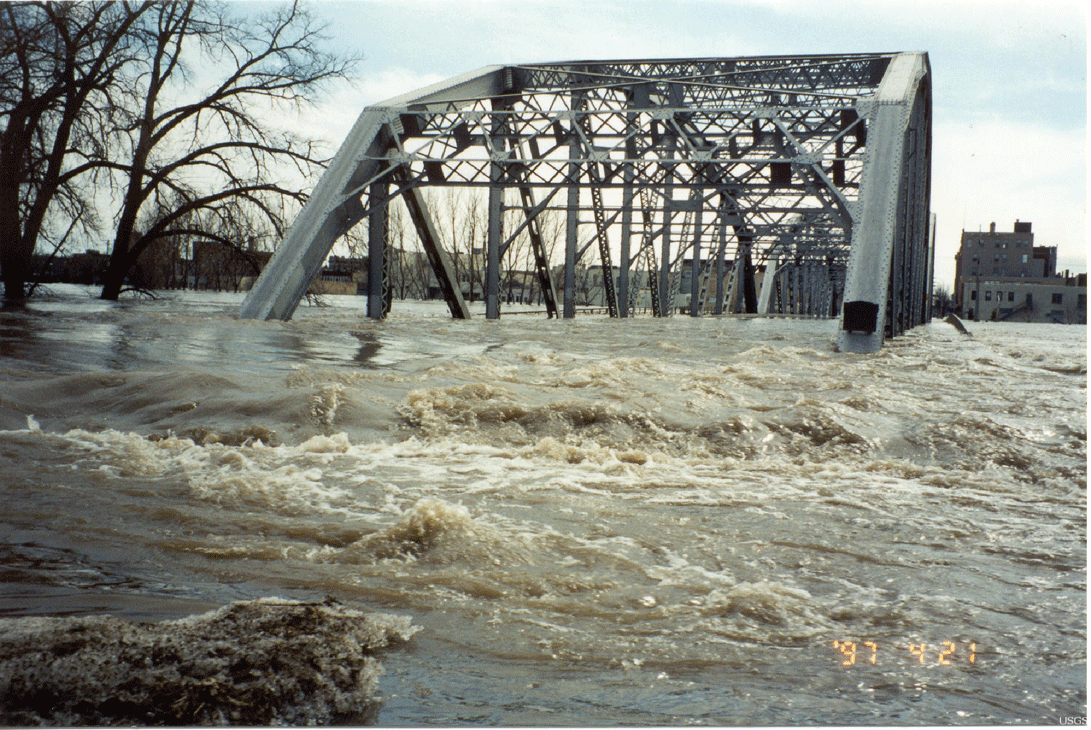
Photograph showing the Sorlie Bridge between Grand Forks, North Dakota, and East Grand Forks, Minnesota, during the 1997 Red River of the North flood. Photograph by the U.S. Geological Survey.
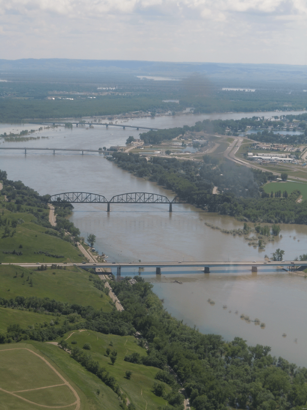
Photograph showing the 2011 flooding of the Missouri River at Bismarck and Mandan, North Dakota. Bridges from top to bottom: Expressway Bridge, Liberty Memorial Bridge, Burlington Northern Santa Fe Railway Bridge, and Interstate 94 Grant Marsh Bridge. Photograph by Joel Galloway, U.S. Geological Survey.
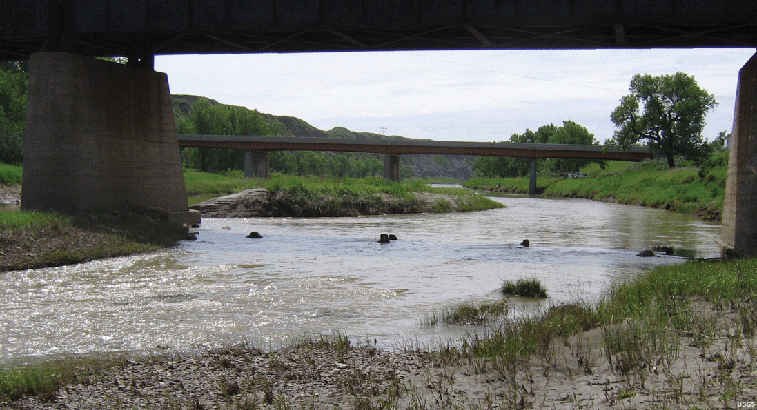
Photograph showing the Little Missouri River at Marmarth, North Dakota, flowing under the railroad and highway bridges with a streamflow of 260 cubic feet per second and a gage height of 2.38 feet. Photograph by Nathan Stroh, U.S. Geological Survey.
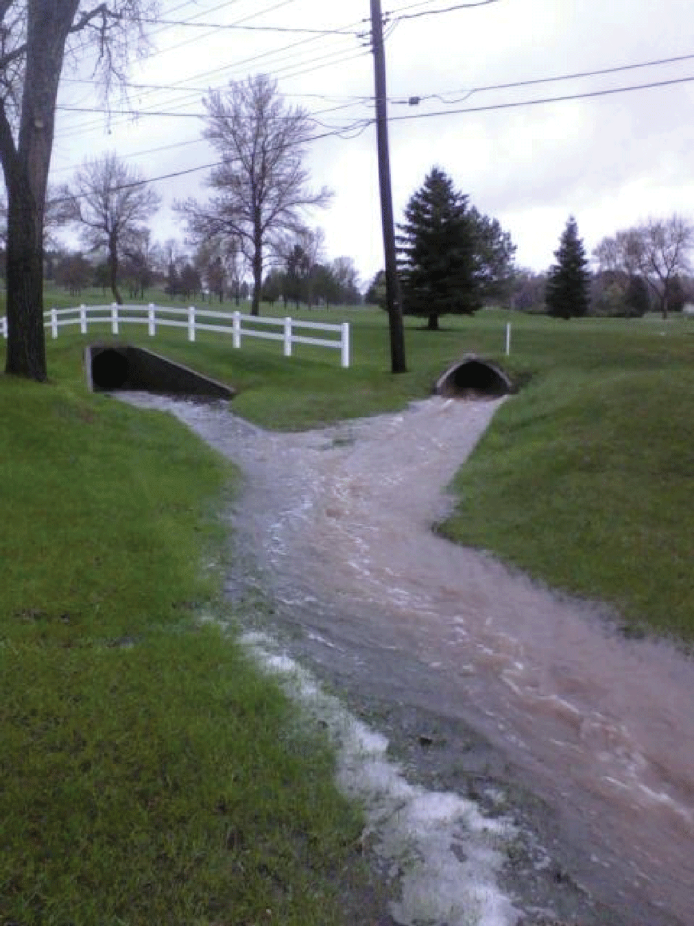
Photograph showing stormwater runoff through culverts in the Arrowhead drainage basin immediately below Arrowhead Country Club during a May 2010 storm event in Rapid City, South Dakota. Runoff from this drainage discharges into Rapid Creek. Photograph by Galen Hoogestraat, U.S. Geological Survey.
Historically, the assumption of stationarity was widely accepted until increased awareness of climatic persistence—extended periods of wet or dry conditions—and concerns over climate and land-use changes prompted a reassessment (Milly and others, 2008; Lins and Cohn, 2011; Stedinger and Griffis, 2011). When the long-term mean flood at a particular site or the variability in flooding changes gradually or abruptly, the time series is considered nonstationary. More generally, nonstationarity refers to changes in the parameters of a time series, and in the context of flood frequency and Bulletin 17C, those parameters are mean, standard deviation, and skew. Nonstationarity can arise from numerous factors, including flow regulation, natural climate variability, climate change, and land-use change.
Bulletin 17C does not offer guidance on addressing nonstationarities or incorporating changing conditions when estimating floods (England and others, 2018). Nevertheless, failing to consider climatic and land-use changes that cause abrupt or gradual changes in flood regimes can result in a poor representation of the true flood risk. Bulletin 17C does identify a need for additional flood-frequency studies that incorporate changing climate or basin characteristics into the analysis (England and others, 2018).
In response to the recent reassessment of the assumption of stationarity and the lack of guidance in Bulletin 17C, the USGS, in collaboration with the Illinois Department of Transportation, Iowa Department of Transportation, Michigan Department of Transportation, Minnesota Department of Transportation, Missouri Department of Transportation, Montana Department of Natural Resources and Conservation, North Dakota Department of Water Resources, South Dakota Department of Transportation, and Wisconsin Department of Transportation, began a study across nine States in the north-central United States (Marti and others, 2023). This study area features diverse physical features, climate, and land use. Variations in elevation, soils, and climate substantially affect the magnitude and timing of peak flows. As shown in figure 5, parts of the study area have contributing drainage areas in Canada and in States that were not part of the study. Many streamgage selection methods use prescreened lists of sites, such as the Geospatial Attributes of Gages for Evaluating Streamflow, Version II (GAGES-II), dataset (Falcone, 2011), that leave out streamgages with parts of their drainage area in Canada because of a lack of unified climate, land-use, and other ancillary data (for example, refer to Ryberg [2022]). However, such data screening leaves out some long-term streamgages in this study area, so we included streamgages with drainage areas outside the nine-State boundary, including areas in Canada.
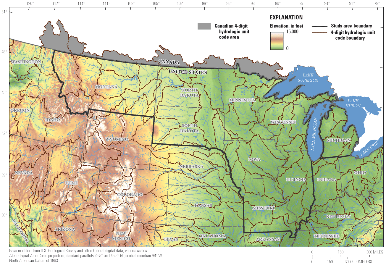
Map showing topography and hydrography of the study area in the north-central United States (modified from fig. 1 of Ryberg and others [2024]).
The first phase of the study summarized how variability in hydrology and climate affects the temporal and spatial distributions of peak-flow data at unregulated sites (Ryberg and others, 2024). The second phase examined changes in seasonality (Barth and others, 2025) and land-use changes related to urbanization (Over and others, 2025) and tile drainage (Podzorski and Ryberg, 2025). These hydrology, climate, and land-use studies are summarized in the following sections.
Hydroclimatic Study
Hydroclimatology “was defined by Langbein (1967) as the study of the influence of climate upon the waters of the land” (Wendland, 1987, p. 497). Precipitation, temperature, evapotranspiration, and imbalances between them are the hydroclimate. Along with physical characteristics like soils and topography, the hydroclimate underlies floods and droughts (Shelton, 2008). The physical characteristics and the hydroclimatology of the study area are diverse. These factors, along with human modifications, affect the peak-flow regime, or the distribution and characteristics of peak flows in a basin (Whipple and others, 2017; Burn and Whitfield, 2023). In some areas, peak-flow regimes are clearly dominated by snowmelt (fig. 6); in other areas, peak-flow regimes are strongly affected by rainfall in spring or summer; and in some areas, peak flows are the result of snowmelt and rain (fig. 7).
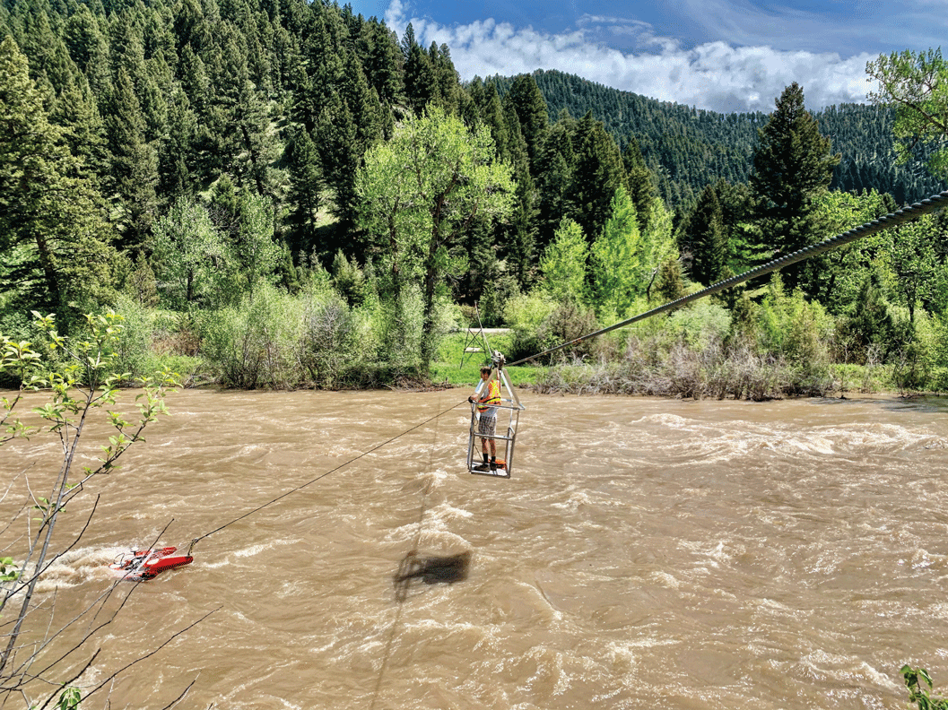
Photograph showing a hydrologic technician making a high-flow measurement during a snowmelt event on the Gallatin River near Gallatin Gateway, Montana. Photograph by Brett Price, U.S. Geological Survey.
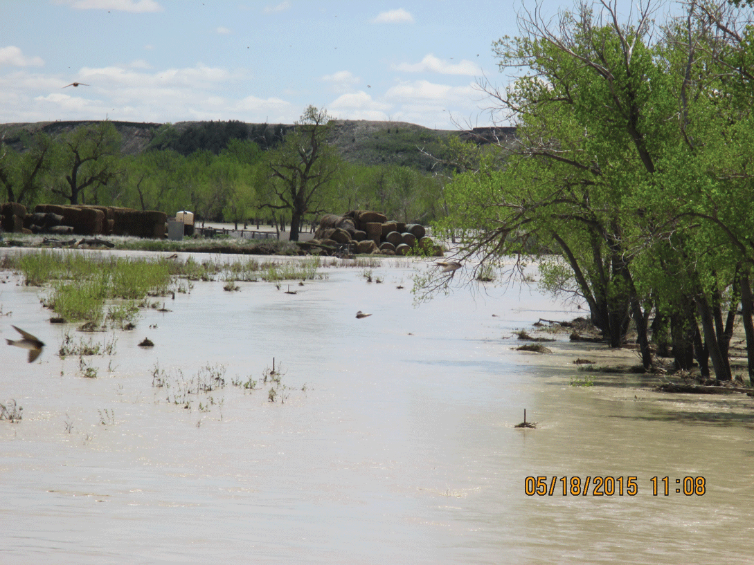
Photograph showing flooding on the White River near Kadoka, South Dakota (U.S. Geological Survey streamgage 06447000). The gage house is left of center near hay bales. Streamflow at this site was measured by the U.S. Geological Survey as about 26,000 cubic feet per second on May 18, 2015. Major flooding was observed on the White River in South Dakota in May 2015 after snow and rain events in western South Dakota. Photograph by Brian Engle, U.S. Geological Survey.
Long-term changes—gradual and abrupt—have been documented in peak flow in the study area; downward trends in the western part of the study area (Sando and others, 2022; Knapp and others, 2023), and upward trends in much of the eastern part of the study area (Levin and Holtschlag, 2022; Knapp and others, 2023). These changes have been attributed to short- and long-term climate patterns and land-use changes (Levin and Holtschlag, 2022; Sando and others, 2022), demonstrating the applicability of concerns about nonstationarity in peak flows in the study area.
Hydroclimatic change and variability were analyzed using peak flow (the maximum instantaneous streamflow values recorded at a particular site for the entire water year [the period from October 1 to September 30 that is designated by the year in which it ends], also called the annual maximum series or AMS), daily mean streamflow (daily streamflow), and climate metrics. Climate metrics analyzed included monthly time series estimates of temperature, precipitation, potential evapotranspiration, actual evapotranspiration, rainfall, snowfall, soil moisture storage, snow water equivalent, and runoff. The precipitation and temperature values are observed data obtained from the NClimGrid dataset (Vose and others, 2015). All other monthly time series are modeled outputs from a monthly water-balance model for 1900–2020 (Wieczorek and others, 2022). All climate metrics were averaged over the contributing drainage area for each streamgage in the study to create basin-average values. The climate metric analysis included areas in bordering States; however, because monthly water-balance model data are only available within the United States, the average is computed only for the area inside the United States. The fraction of each basin that is within the United States is recorded for the analyst to consider in interpreting the climatic results (this information is provided in an associated USGS data release [Marti and others, 2024a]).
The streamflow and climate data were analyzed in parallel for comparative purposes. All data were analyzed across four periods: (1) a 100-year period, 1921–2020; (2) a 75-year period, 1946–2020; (3) a 50-year period, 1971–2020; (4) and a 30-year period, 1991–2020 (Ryberg and others, 2024). To focus on hydroclimatic variability, a data-informed, regionally consistent approach of screening candidate streamgages for substantial regulation or water diversions was necessary. The method used consisted of examining existing streamflow qualification codes and using a dam impact metric to determine whether a streamgage was suitable for our analysis (Marti and Ryberg, 2023). The number of streamgages used varies with period, and few sites were in the 100-year period compared to the 30-year period. In addition, the number of streamgages with daily streamflow is less than the number with sufficient peak flow for this study. Therefore, some site-trend period combinations have peak-flow and daily flow analyses, but others have only peak-flow analyses. The climate analyses were completed for all streamgages included in the study.
Literature review, data compilation, and analyses were completed as a consistent whole for the nine-State study. These steps are documented in chapter A (Ryberg and others, 2024) of a multichapter USGS Scientific Investigations Report (Ryberg, 2024a). An array of statistical and graphical analyses was used to investigate peak flow, daily streamflow, and the climate metrics, including testing for monotonic trends and change points. Monotonic trends are gradual increases or decreases in peak flow that are not necessarily linear. Monotonic trends can have some curvature, as opposed to a straight-line representation of the trend (as in linear regression), but the trend direction is always upward or always downward (a line representing the pattern in the data cannot be s-shaped; Helsel and others, 2020). Change points are abrupt changes, sometimes called step trends or breakpoints, in the central tendency of floods or in the variability of floods.
Daily streamflow was used to study floods through peaks-over-threshold (POT) analysis using partial-duration flood series. A partial-duration flood series is a list of all flows that exceed a chosen base stage or discharge, regardless of the number of peaks resulting during a water year. This partial-duration flood series also is referred to as “floods above a base” (Langbein and Iseri, 1960; England and others, 2018). Because of a lack of general guidelines for setting a threshold for the floods above a base, this POT approach tends to be underused compared to analyses that use annual maximum floods based on water year. The primary challenge with the POT approach is meeting the independence criteria between candidate daily flood events. In this study, the approach described in Neri and others (2019) was applied to complete a POT analysis with, on average, two events per year (POT2) and four events per year (POT4) and no more than one event in a time window defined as 5 days plus the logarithm of the drainage area in square miles (|log (drainage area) +5 days|).
The code, text documentation, and numerical and graphical analysis results for peak flow and daily streamflow were combined in R Markdown documents that are available in an associated USGS data release (Marti and others, 2024b). Similarly, numerical and graphical analysis results for the climate analyses are combined in R Markdown documents (Marti and others, 2024b). R Markdown documents are reproducible “notebook interfaces” that combine code, narrative, and graphics (RStudio, 2020). Once the data release files are downloaded, the Markdown documents allow users to navigate through the results and view graphical depictions of analyses at every site in the study. An introduction to the entire study area and detailed descriptions of the statistical and graphical analyses were provided in chapter A (Ryberg and others, 2024) of a multichapter USGS Scientific Investigations Report (Ryberg, 2024a). Interpretations of the results were reported in separate chapters for each of the nine States (Barth and Sando, 2024; Levin, 2024a, b; Marti and Heimann, 2024; Marti and Over, 2024; O’Shea, 2024; Ryberg and Williams-Sether, 2025; Sando and others, 2025; Williams-Sether and Sanocki, 2025).
Presentation of Statistical Significance
For all statistical hypothesis tests, the probability (p) values are reported in an associated data release (Marti and others, 2024b). When the results of statistical tests for trends are mapped, the trends are presented using a likelihood approach, an alternative to simply reporting significant trends with an arbitrary cutoff point. Trend likelihood values were determined using the p-value reported by each test using the following equation: trend likelihood=1–(p-value/2). When the trend is likely upward or likely downward, the trend likelihood value associated with the trend is between 0.85 and 1.0; that is, the chance of the trend going in the specified direction is at least 85 out of 100. When the trend is somewhat likely upward or somewhat likely downward, the trend likelihood value associated with the trend is between 0.70 and 0.85; that is, the chance of the trend going in the specified direction is between 70 and 85 out of 100. When the trend is about as likely as not, the trend likelihood value associated with the trend is less than 0.70; that is, the chance of the trend being either upward or downward is less than 70 out of 100 (refer to Ryberg and others [2024] for additional details).
State-Based Summaries
Summaries of interpretations by State follow. Notably, not all analyses completed are summarized here, and although many spatial and temporal patterns transcend State boundaries, the patterns observed in each State are different; therefore, the State summaries have differing foci. For example, not all summaries include results from the POT analyses.
Many more interpretations are available for each State in the State-based chapters (Barth and Sando, 2024; Levin, 2024a, b; Marti and Heimann, 2024; Marti and Over, 2024; O’Shea, 2024; Ryberg and Williams-Sether, 2025; Sando and others, 2025; Williams-Sether and Sanocki, 2025). In addition, all numerical results and graphics generated for each site-trend period analysis are available for further use and interpretation in an associated data release (Marti and others, 2024b).
Illinois Summary
Peak-streamflow magnitude has generally increased at streamgages across Illinois, and most streamgages in the 100- and 75-year trend periods had a likely or somewhat likely upward monotonic trend in the peak-streamflow median magnitude (fig. 8), including the Sangamon River (fig. 9). Most streamgages in the 50- and 30-year trend periods have upward trends but are clustered in the northern and southern parts of the State, and a larger fraction of streamgages in the 50- and 30-year trend periods do not have a trend than in the longer trend periods (Marti and Over, 2024). The median trend magnitudes (normalized by median peak flow) equate to a 41-percent increase over 100 years, a 35-percent increase over 75 years, a 26-percent increase over 50 years, and a 23-percent increase over 30 years (Marti and Over, 2024).
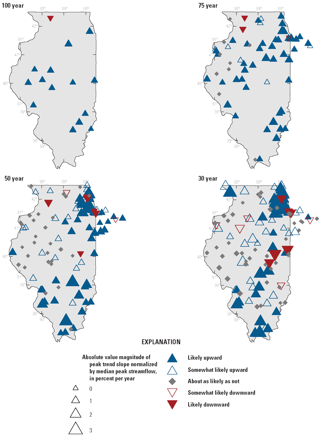
Maps showing likelihoods and magnitudes of monotonic trends in peak-streamflow magnitude in Illinois for all trend periods (modified from fig. 10 of Marti and Over [2024]).
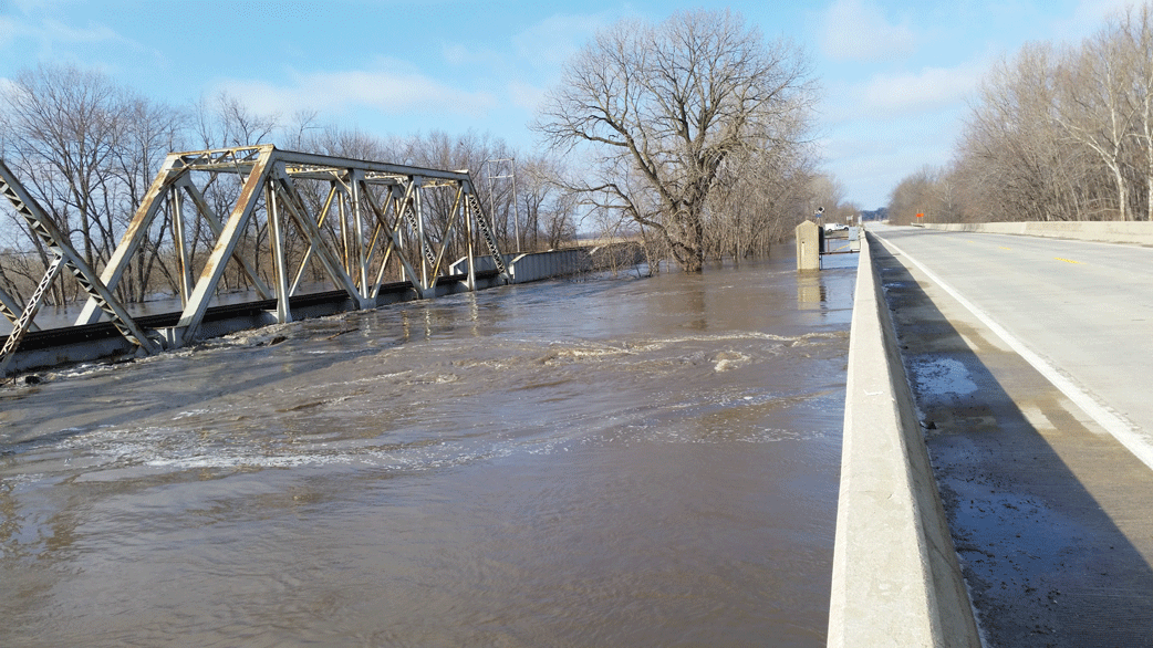
Photograph showing flooding conditions at U.S. Geological Survey streamgage 05583000 (Sangamon River near Oakford, Illinois) on January 1, 2016. Daily mean streamflow on this date was measured as 71,700 cubic feet per second. Photograph by Perry Draper, U.S. Geological Survey.
Streamgages with trends often also have change points (a change point is an abrupt rather than gradual change in peak flow). More than two-thirds of streamgages in the 100- and 75-year trend periods had a monotonic trend and change point in peak flows; the shorter trend periods had a smaller percentage of overlap (Marti and others, 2024b). The change-point results generally mimic those of the monotonic trends, and upward change points were detected throughout most of the State at the 100- and 75-year trend periods and in northern and southern Illinois at the 50- and 30-year trend periods. Increases in the frequency of peak flows, evaluated using a POT analysis, were observed in similar areas as increases in peak-streamflow magnitude (Marti and others, 2024b). Changes in peak flow in Illinois seem to be driven by increasing annual and seasonal precipitation (fig. 10), which increases soil water moisture and runoff. Precipitation has increased despite higher temperatures, which are driving increases in potential evapotranspiration (Marti and Over, 2024).
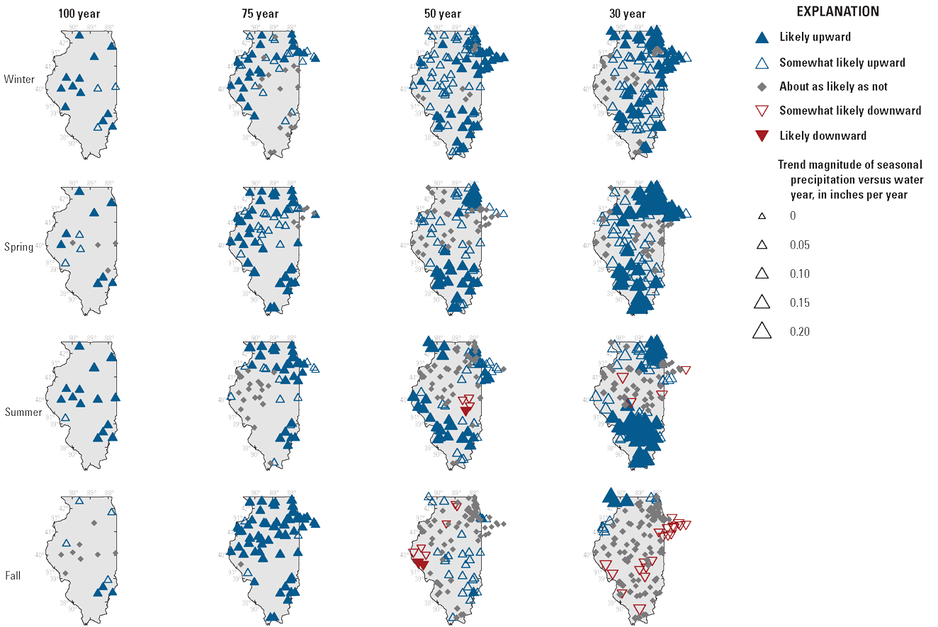
Maps showing likelihoods and magnitudes of trends in seasonal precipitation in study basins in Illinois for all trend periods and seasons (winter, December–February; spring, March–May; summer, June–August; and fall, September–November). Symbols are mapped at the outlets of basins (that is, at the location of the streamgage; modified from fig. 26 of Marti and Over [2024]).
Iowa Summary
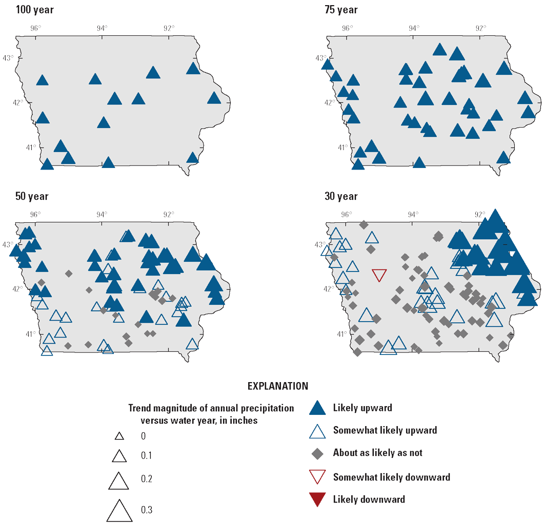
Nearly two-thirds of streamgages included in the study for Iowa have indications of nonstationarity, and more than half have an upward trend in each of the four trend periods (fig. 11). The magnitude of these trends is substantial; median trend magnitude (normalized by the median peak flow) equates to a 48-percent increase over 100 years, a 21.8-percent increase over 75 years, a 25.5-percent increase over 50 years, and a 33-percent increase over 30 years (O’Shea, 2024). A cluster of streamgages in southwestern Iowa had largely downward trends for the 75- and 50-year trend periods (fig. 11). The USGS streamgage Big Sioux River at Akron, Iowa (06485500), on the Iowa-South Dakota border is part of the area in northwestern Iowa with increasing trends in magnitude (figs. 11 and 12).
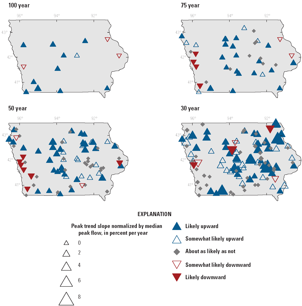
Maps showing likelihoods and magnitudes of monotonic trends in peak-streamflow magnitude in Iowa for all trend periods (modified from fig. 10 of O’Shea [2024]).
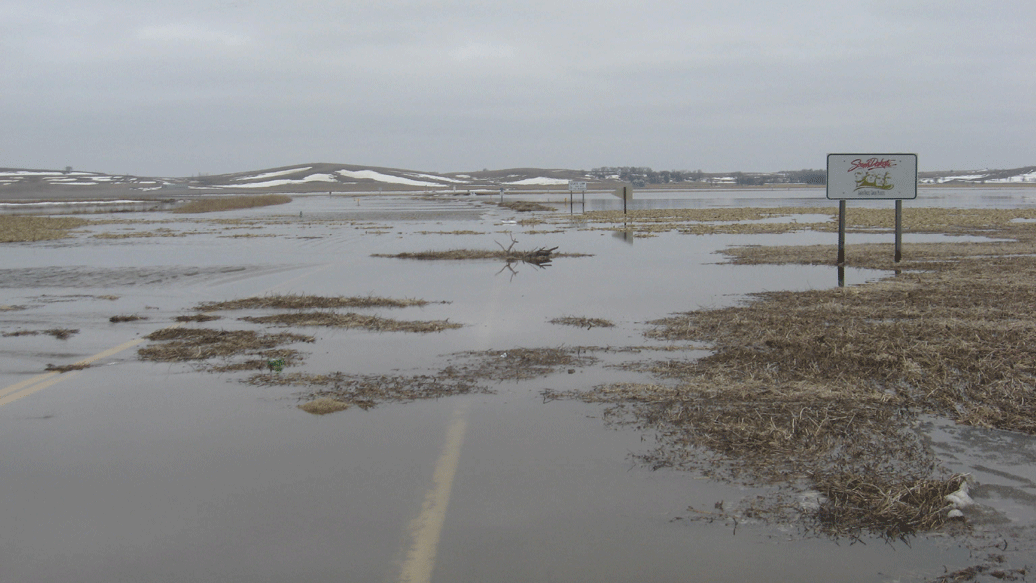
Photograph showing flooding conditions at U.S. Geological Survey streamgage 06485500 (Big Sioux River at Akron, Iowa) on March 17, 2010. Daily mean streamflow on this date was more than 30,000 cubic feet per second. Photograph by Nate Stevens, U.S. Geological Survey.
Trends in annual and seasonal precipitation, particularly for the spring and summer, correspond well to the upward monotonic trends at most USGS streamgages in Iowa. Exceptions include southwestern Iowa where downward trends in peak flow are more common despite mostly upward trends in precipitation for the region (fig. 13). Decreasing trends in the accumulation of snow, as measured by the snow water equivalent, as well as changes in the timing of peak flow indicate a shift away from springtime snowmelt-driven floods toward short but intense precipitation-driven flooding in Iowa (Marti and others, 2024b; O’Shea, 2024).
Maps showing likelihoods and magnitudes of trends in annual precipitation in study basins in Iowa for all trend periods (modified from fig. 27 of O’Shea [2024]).
Michigan Summary
Trends (fig. 14) and change points (refer to the associated data release [Marti and others 2024b]) in peak flow were detected across the State of Michigan (Levin, 2024a). Trends and change points in peak flow were primarily upward in the lower peninsula across all time periods (the upward trends represent gradual increases and the upward change points represent abrupt increases in the central tendency of the peak flows), such as for the 30-year period for the Rifle River (fig. 15; refer to results in the associated data release [Marti and others, 2024b]) with some isolated downward changes. In the upper peninsula, trends and change points were downward for the 75- and 50-year time periods but upward or neutral for the 30-year period. Shifts in the timing of peak flows were identified with a shift toward later peaks in the southern half of the lower peninsula, and a shift toward earlier peaks in the eastern and northern areas of the lower peninsula. For streamgages with upward trends in peak-flow timing in the 75-year period, the peak flow shifted an average of 23 days later in the spring during the analysis period (Levin, 2024a; Marti and others, 2024b).
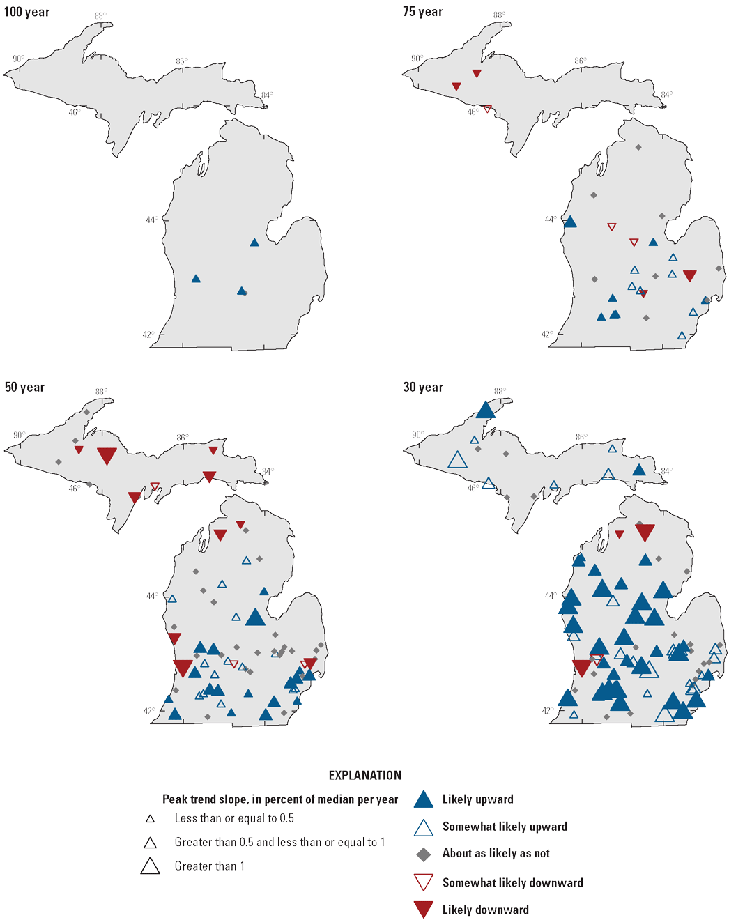
Maps showing magnitudes and likelihoods of monotonic trends in annual peak-streamflow trends at selected U.S. Geological Survey streamgages in Michigan for four analysis periods ending in water year 2020 (modified from fig. 10 of Levin [2024a]). [A water year is the period from October 1 to September 30 and is designated by the year in which it ends]
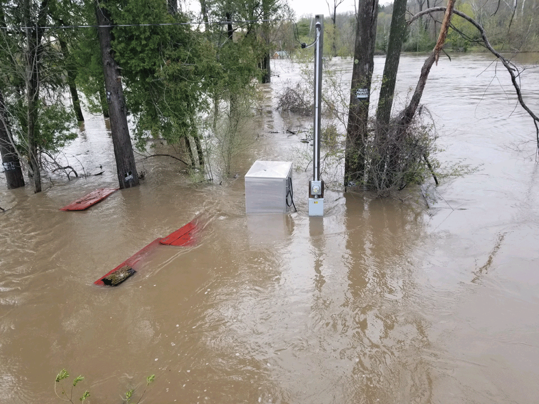
Photograph showing U.S. Geological Survey nutrient sampler submerged during major flooding on the Rifle River, Michigan, in May 2020. This site is near U.S. Geological Survey streamgage 04142000 (Rifle River near Sterling, Michigan). Photograph by Tom Weaver, U.S. Geological Survey.
Changes in climate during the periods of analysis point to wetter conditions overall and are likely driving increases in streamflow (fig. 16). Annual precipitation increased at nearly every streamgage in the study, and the largest in magnitude was in winter and spring. Temperature increased statewide, and most temperature trends began in the mid-1970s. Temperature trends were generally strongest in fall and winter and weakest in the spring. Despite widespread increases in annual temperature, modeled potential evapotranspiration to precipitation ratios indicate an overall trend toward wetter conditions in Michigan (Levin, 2024a).
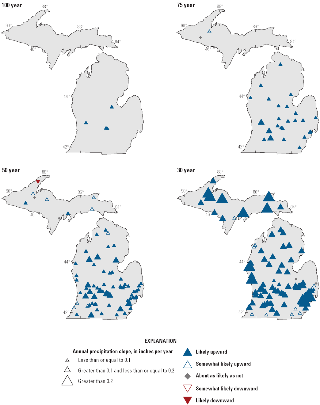
Maps showing magnitudes and likelihoods of monotonic trends in annual precipitation at selected U.S. Geological Survey streamgages in Michigan for four analysis periods ending in water year 2020 (modified from fig. 21 of Levin [2024a]). [A water year is the period from October 1 to September 30 and is designated by the year in which it ends]
Minnesota Summary
Upward monotonic trends in peak flow were detected northwest to southeast in the 100-, 75-, and 50-year analysis periods and north to south in the 30-year analysis period (fig. 17). Downward monotonic trends were detected mainly in the northeastern and southeastern areas of Minnesota. Change points in the median peak flow were detected during 1959 to 2003, and most detections were in the early to mid-1990s. Some sites indicated increases in the number of peaks above a threshold in the 1990s as well, including the Roseau River below South Fork near Malung, Minnesota (USGS streamgage 05104500; fig. 18). The spatial patterns in change points were like those for monotonic trends. Trends in peak-flow timing indicated that peak flows are later in the water year mainly in the southern part of Minnesota and earlier in the water year mainly in the northern part of Minnesota (Williams-Sether and Sanocki, 2025).
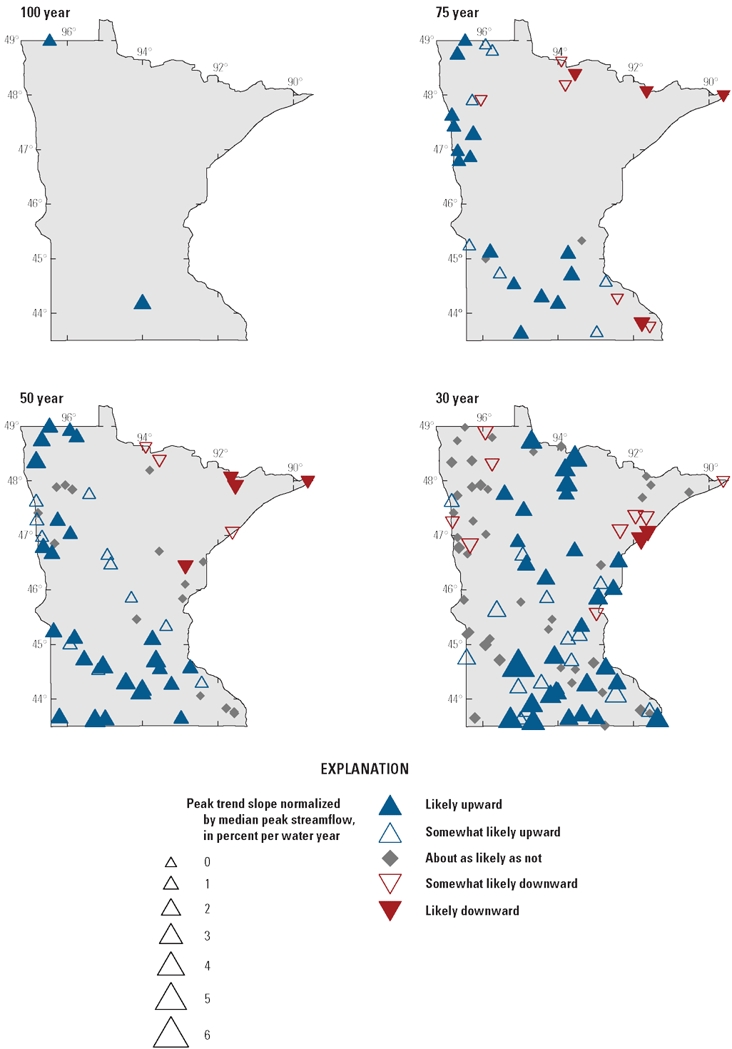
Maps showing likelihoods and magnitudes of monotonic trends in peak-streamflow magnitude in Minnesota for all trend periods (modified from fig. 11 of Williams-Sether and Sanocki [2025]).
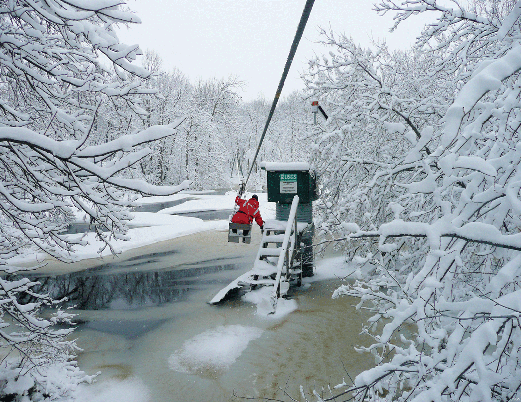
Photograph showing a U.S. Geological Survey (USGS) hydrologic technician using a cable car to access USGS streamgage 05104500 (Roseau River below South Fork near Malung, Minnesota) on March 26, 2009. Photograph by Brett Savage, USGS.
Changes in climate, in general, point to wetter conditions in the southern areas of Minnesota and drier conditions in the northern areas of Minnesota. Annual precipitation was determined to be increasing northwest to southeast in the 100-, 75-, and 50-year analysis periods and in the east in the 30-year analysis period (fig. 19). In contrast, areas in the north and northwest in the 50- and 30-year analysis periods indicated decreasing annual precipitation (fig. 19). These differences in trend direction may have several causes. Trend methods are sensitive to periods of record because of persistence, especially at the beginning or end of the record, from naturally occurring quasi-periodic hydroclimatic processes (Cohn and Lins, 2005). If a series of dry years was at the end of the 30-year period, that would strongly affect the detection of a downward trend. Continued observations will indicate whether that downward trend persists.
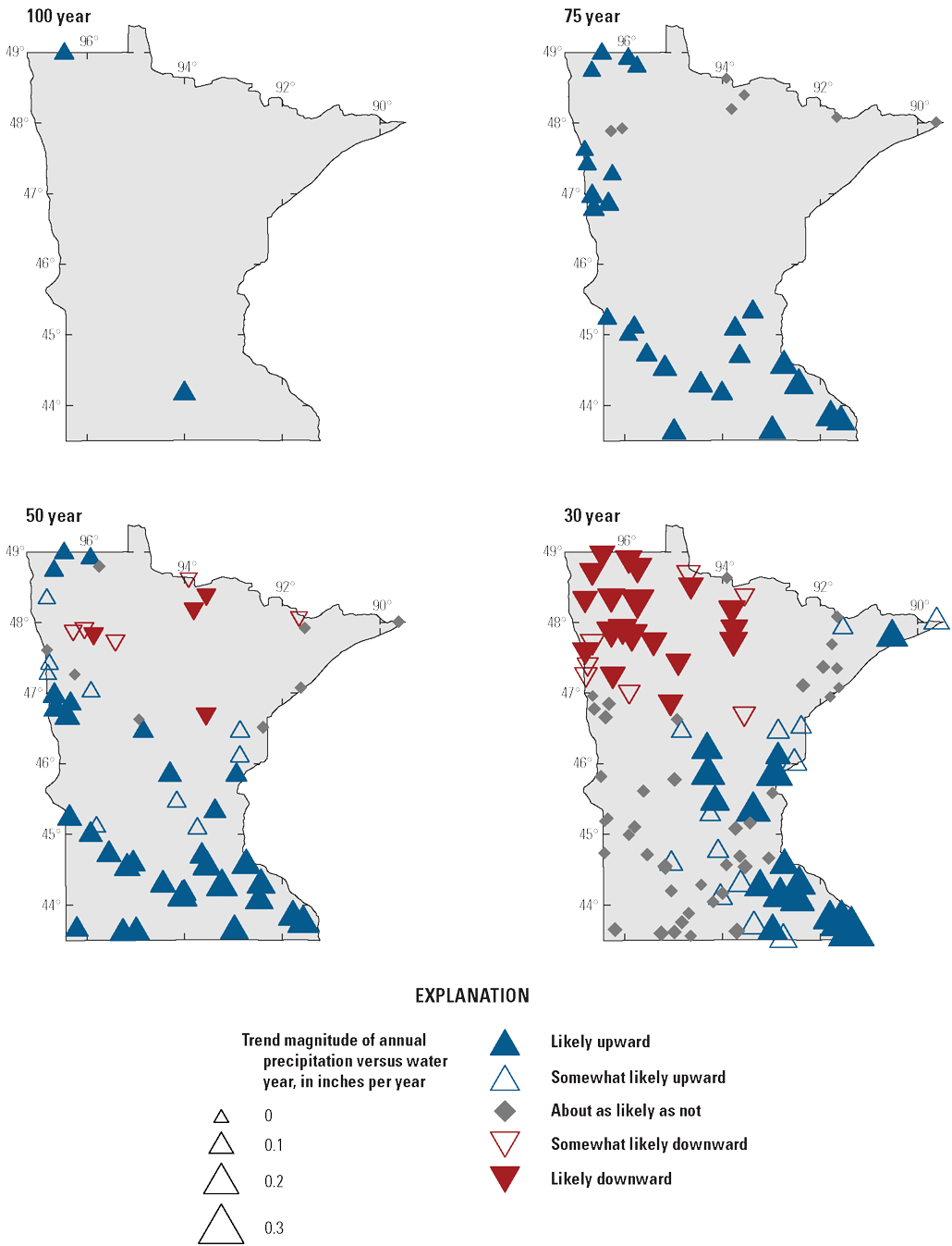
Maps showing magnitudes and likelihoods of monotonic trends in annual precipitation at selected U.S. Geological Survey streamgages in Minnesota for four analysis periods ending in water year 2020 (modified from fig. 23 of Williams-Sether and Sanocki [2025]). [A water year is the period from October 1 to September 30 and is designated by the year in which it ends]
Notable patterns in other climate metrics were detected in Minnesota. The graphics are not shown here (refer to Williams-Sether and Sanocki [2025] for graphics) but are summarized as follows. Annual snowfall was determined to be mostly decreasing across Minnesota except in areas in the extreme northeast, where annual snowfall was determined to be increasing. Decreases in annual potential evapotranspiration were detected mainly in the southern half of Minnesota, and increases were detected in the northern half of Minnesota. Annual soil moisture increased in the southern area of Minnesota and decreased in the northern area of the Minnesota in the 100-, 75-, and 50-year analysis periods. Annual soil moisture decreased in the northern and eastern parts of the Minnesota in the 30-year analysis period (Williams-Sether and Sanocki, 2025).
Missouri Summary
Peak-streamflow magnitude has increased at most streamgages across the State of Missouri for the 100-, 75-, and 50-year trend periods (fig. 20). At least 77 percent of streamgages in the 100-, 75-, and 50-year trend periods had an upward monotonic trend in peak-streamflow magnitude, and no streamgages had a downward trend, including the Meramec River (fig. 21). In the 30-year trend period, 37 percent of streamgages had an upward trend, clustered mostly in southwestern Missouri, and most streamgages in northern and southeastern Missouri had no trend. The median trend magnitude (normalized by the median peak flow) equates to a 40-percent increase in the median peak flow over 100 years, a 40-percent increase over 75 years, a 28-percent increase over 50 years, and a 10-percent increase over 30 years (Marti and Heimann, 2024). Patterns in change points in peak-streamflow magnitude generally match patterns in the monotonic trends with upward change points throughout most of the State at the 100- and 75-year trend periods (Marti and others, 2024b). The frequency of large streamflows has increased at some streamgages and trend periods in Missouri, but these increases are not as widespread as the increases in peak-streamflow magnitude (Marti and Heimann, 2024).
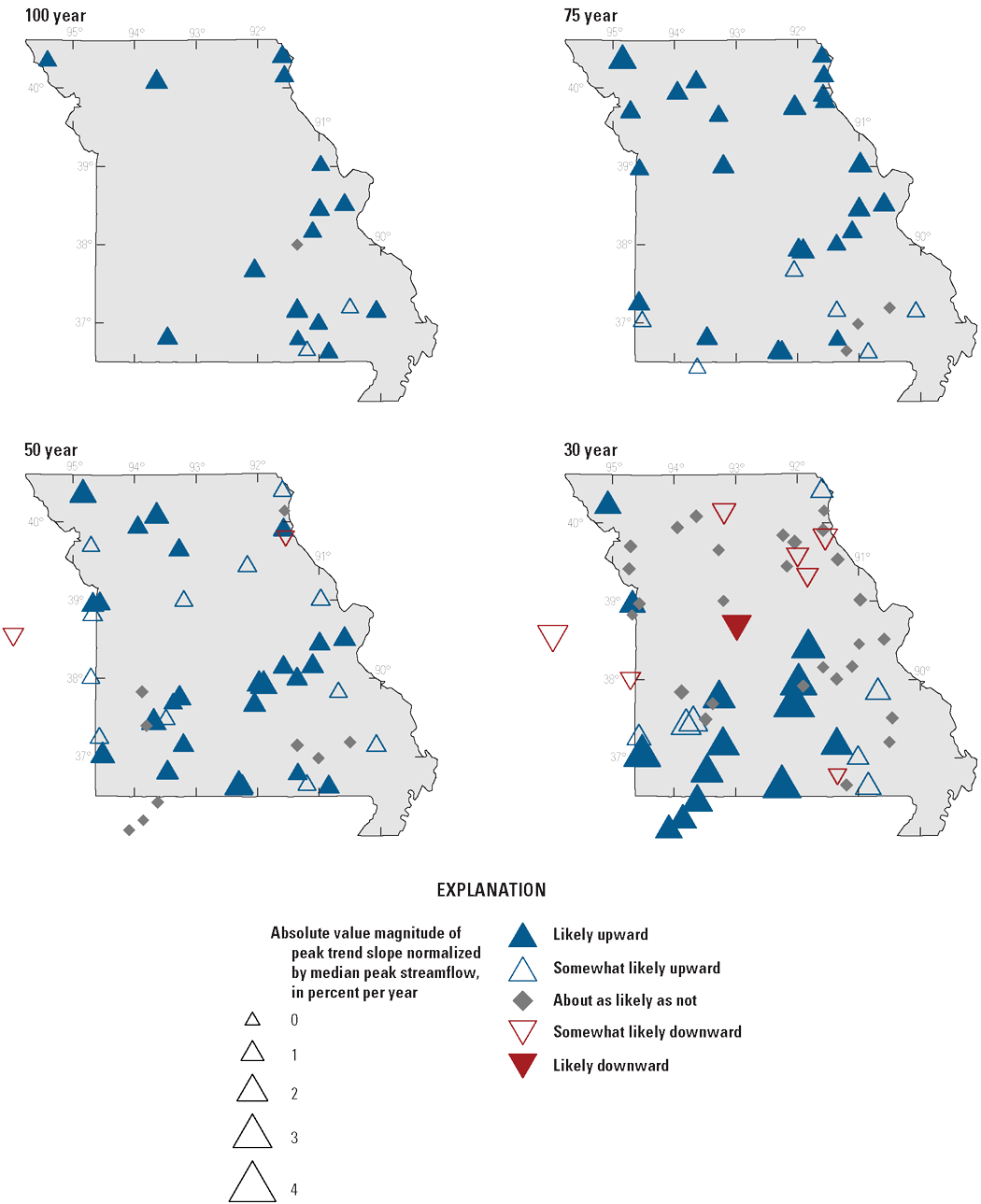
Maps showing likelihoods and magnitudes of monotonic trends in peak-streamflow magnitude in Missouri for all trend periods (modified from fig. 10 of Marti and Heimann [2024]).
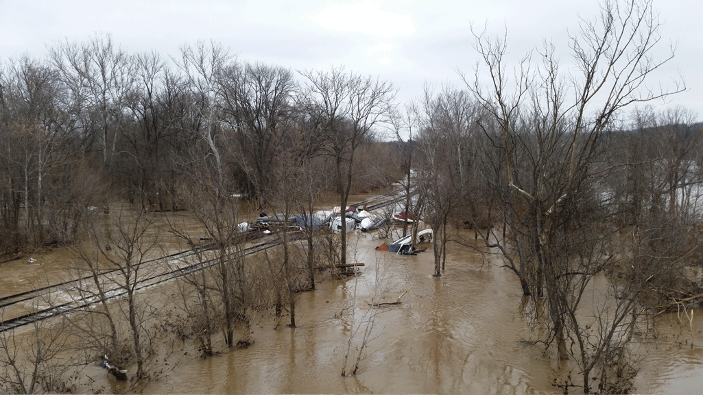
Photograph showing record flooding on the Meramec River in Eureka, Missouri, on December 30, 2015. In late 2015 and early 2016, unusually large rainfall in the Upper Mississippi River Valley led to substantial flooding in Arkansas, Illinois, Louisiana, Mississippi, Missouri, and Tennessee. Photograph by Miya Barr, U.S. Geological Survey.
Changes in peak flow in Missouri seem to be driven by increasing annual and seasonal precipitation, which increases soil water moisture and runoff (fig. 22). Precipitation has increased despite higher temperatures, which are driving increases in potential evapotranspiration for the 75-, 50-, and 30-year trend periods (Marti and Heimann, 2024).
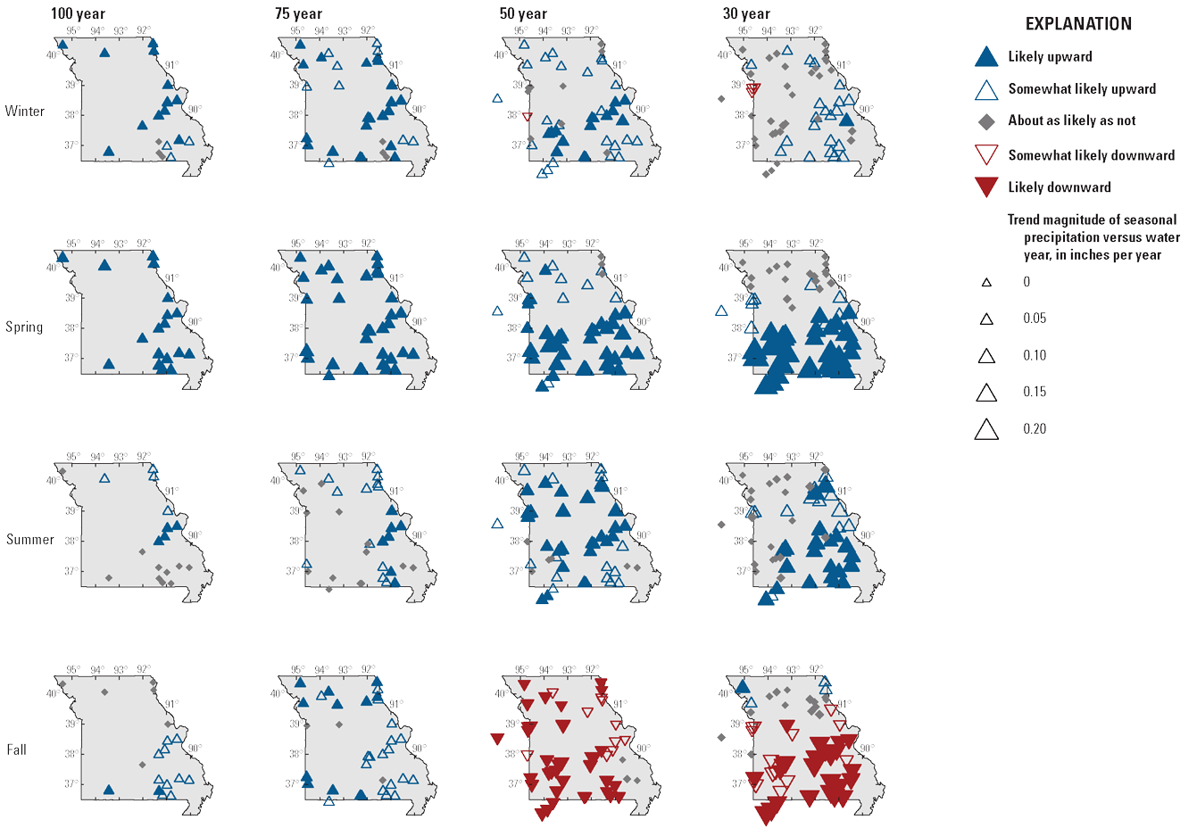
Maps showing likelihoods and magnitudes of trends in seasonal precipitation in study basins in Missouri for all trend periods (winter, December–February; spring, March–May; summer, June–August; and fall, September–November). Symbols are mapped at the outlets of basins (that is, at the location of the streamgage; modified from fig. 26 of Marti and Heimann [2024]).
Montana and Northern Wyoming Summary
Montana and northern Wyoming make up a part of the study area that is geographically diverse with plains in the east to high mountains in the west (fig. 23). As such, the results of nonstationarity analysis for Montana and contributing basins in northern Wyoming are variable (figs. 24A–D and 25A–D). The 30- and 50-year peak-flow change-point results have substantial percentages of trends that are about as likely as not. The general patterns of the peak-flow change-point results and the peak-flow monotonic trend results are quite similar (figs. 24A–D and 25A–D).
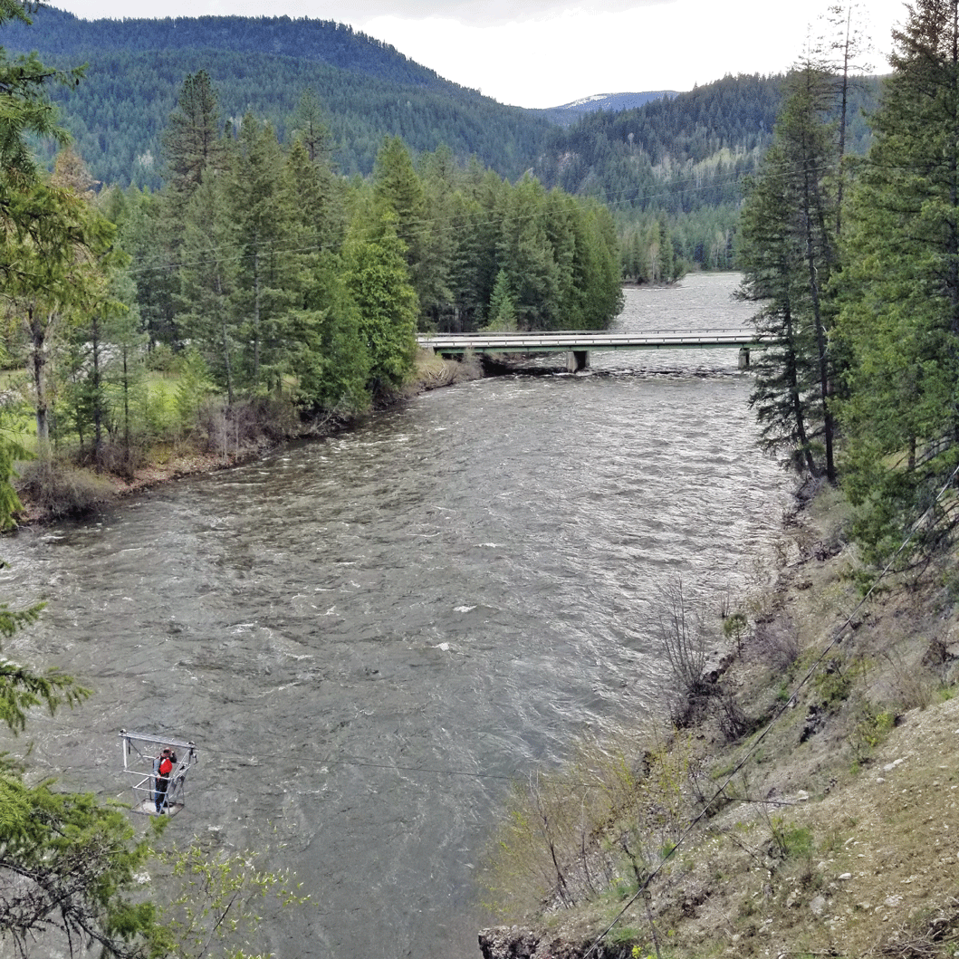
Photograph showing a U.S. Geological Survey hydrologic technician on the cableway over the Yaak River near Troy, Montana. Photograph by Ryan Smith, U.S. Geological Survey.
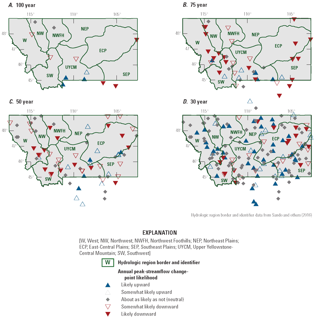
Maps showing annual peak-streamflow change-point likelihoods for streamgages included in the (A) 100-, (B) 75-, (C) 50-, and (D) 30-year analyses in Montana and northern Wyoming (modified from fig. 23 of Sando and others, 2025).
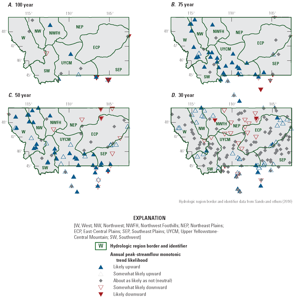
Maps showing annual peak-streamflow monotonic trend likelihoods for streamgages included in the (A) 100-, (B) 75-, (C) 50-, and (D) 30-year analyses in Montana and northern Wyoming (modified from fig. 26 of Sando and others, 2025).
The change points for the 50-, 75-, and 100-year periods are predominantly downward (fig. 24A–C) and are concentrated in the 1970s and 1980s (Sando and others, 2025). The downward 50- and 75-year nonstationarities are associated with mostly upward temperature and potential evapotranspiration to precipitation ratio monotonic trends (Sando and others, 2025). The 30-year peak-flow change-point and monotonic trend results are predominantly neutral and moderately upward, respectively, and proportions of streamgages where peak flows are increasing are about twice as prevalent as streamgages where peak flows are decreasing (figs. 24D and 25D). It is reasonable to conclude that increases in annual precipitation, winter precipitation, and the annual snow to precipitation ratio contributed to the increases in peak flow.
For the 100-year monotonic trend results, three streamgages are likely downward and five are likely upward (fig. 25A). The five likely upward streamgages are in the mountains, and three of the five are in the mountainous headwaters of the Missouri and Yellowstone Rivers. The three likely downward streamgages are in the lower Yellowstone River Basin (Sando and others, 2025). The annual center of volume duration (the number of days between the dates by which 25 percent and 75 percent of the annual streamflow volume has passed a streamgage) decreased for two of the streamgages with likely upward peak-flow trends in the Missouri and Yellowstone River Basins, which could indicate that the snowmelt runoff period is compressing in those mountainous headwaters (refer to the associated data release for graphics showing this compression [Marti and others, 2024b]). Conversely, the annual center of volume duration increased for two of the streamgages with likely downward peak-flow trends, which could indicate an expanding snowmelt runoff period for those streamgages in the lower Yellowstone River Basin (Sando and others, 2025).
The trend analyses cover periods of substantial variability in hydroclimatic conditions: persistent periods of warm and dry conditions with low streamflows and cool and wet conditions with high streamflows (fig. 26). In some cases, small adjustments of about 10 years in the starting point of a given analysis period might provide different results for the same analysis period length. The trend analysis periods should be considered in relation to these hydroclimatic fluctuations (Sando and others, 2025).
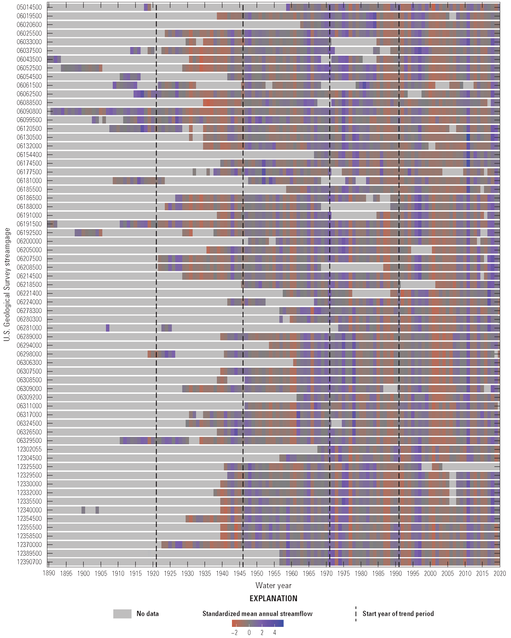
Graph showing standardized departures of annual mean streamflow from long-term mean annual streamflow for 65 selected streamgages in or near Montana (1890–2020; U.S. Geological Survey, 2021). The annual departures were standardized using Z-scores, which are the number and direction of standard deviations away from the long-term mean annual streamflow (modified from fig. 8 of Sando and others 2025). [A water year is the period from October 1 to September 30 and is designated by the year in which it ends]
North Dakota Summary
In summarizing patterns, analysts balance the intersecting objectives of widespread spatial coverage for trends and temporal coverage by using the longest trend period possible. In this study, for the State of North Dakota, the 50-year trend period is the period that balances spatial and temporal coverage best (fig. 27; Ryberg and Williams-Sether, 2025). The pattern of monotonic changes in peak flow in this period can be summarized as increased magnitude in the eastern half of the State and decreased magnitude in the western half of the State. The 100th meridian is an approximate dividing line, a pattern also observed in South Dakota (Barth and Sando, 2024) and more broadly in the Great Plains (Powell, 1879; Stegner, 1954; Knapp and others, 2023).
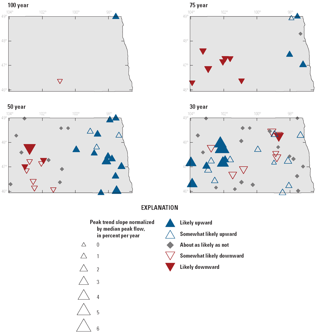
Maps showing likelihoods and magnitudes of monotonic trends in peak-streamflow magnitude in North Dakota for all trend periods (modified from fig. 13 of Ryberg and Williams-Sether [2025]).
For the 50-year period, the ratio of annual snowfall to annual precipitation declined across the State (Ryberg and Williams-Sether, 2025). This pattern of decreased annual snowfall as a fraction of annual precipitation can be observed across the Northern Hemisphere; however, like in North Dakota, the resulting streamflow variation is complex (Han and others, 2024; Ryberg, 2024b).
Eastern parts of the State are in a snow climate and typically have a pattern indicating that the highest frequency of occurrence of peak flow is in the spring, indicative of snowmelt (fig. 28A and B; Ryberg and others, 2016). Snowmelt peaks tend to be larger than rain-generated peaks; however, in the eastern part of the State, flood magnitude increased but snow as part of total precipitation declined. This observation can be explained by changes in annual and seasonal precipitation. In the 50-year trend period, annual precipitation increased; therefore, even if snow amounts held steady, the ratio of snow to total precipitation would decline. In addition, summer and fall precipitation increased (fig. 29), but the ratio of annual potential evapotranspiration and precipitation declined (Ryberg and Williams-Sether, 2025). Greater than normal precipitation in the fall can increase soil moisture, resulting in increased soil moisture in the eastern part of the State. Moisture-surplus conditions carry over into the spring and can increase runoff and flood risk (Ryberg and others, 2014). Evapotranspiration, which is controlled in part by temperature, is a primary part of the water balance along with precipitation and runoff, and results indicate that, despite increased temperatures, the ratio of annual potential evapotranspiration and precipitation has decreased. This decrease indicates that precipitation is a larger driver of observed peak-streamflow trends in the east than temperature or evapotranspiration (Marti and others, 2024b; Ryberg and Williams-Sether, 2025).
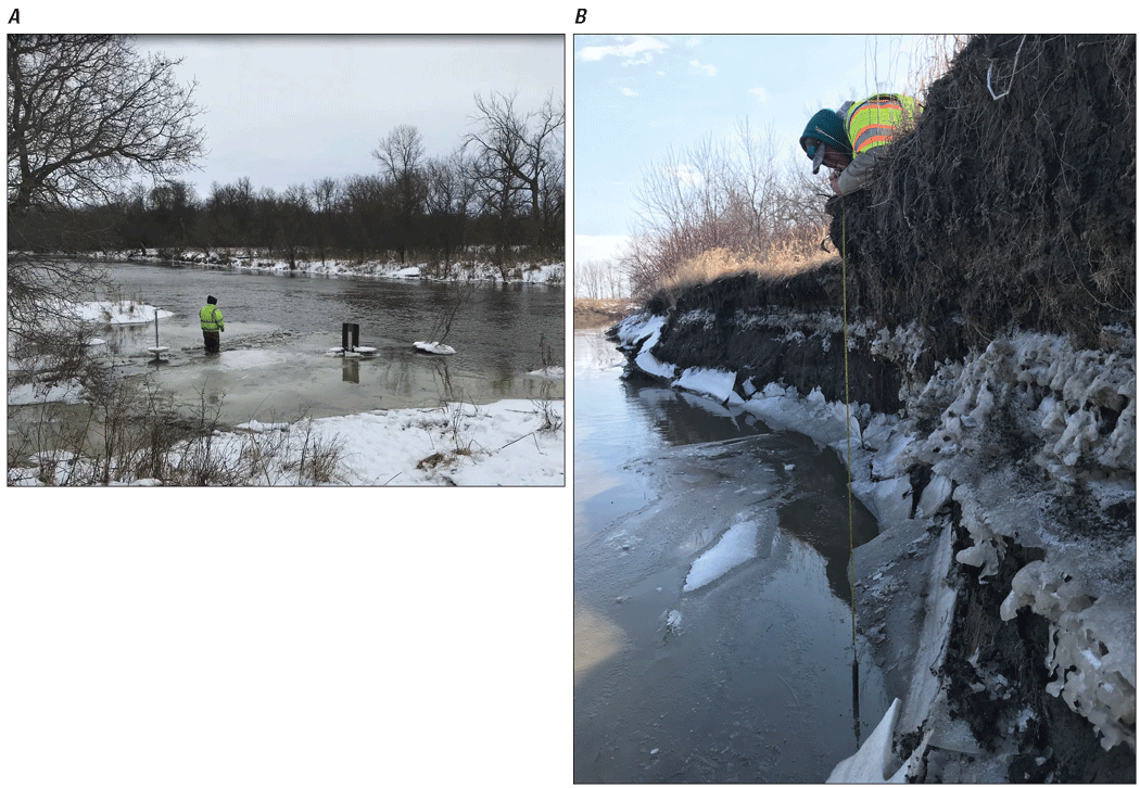
Photographs showing (A) a U.S. Geological Survey (USGS) hydrologist wading out in freezing waters to collect flood data on the Sheyenne River near Cooperstown, North Dakota, and (B) a USGS hydrologic technician measuring a high-water mark on the Pembina River at Neche, North Dakota. Photographs by (A) David Baude and (B) Ernie McCoy, USGS.
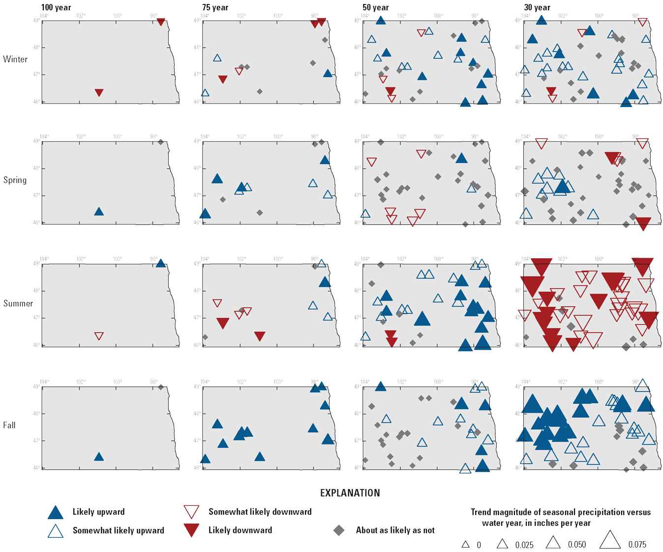
Maps showing likelihoods and magnitudes of trends in seasonal precipitation in study basins in North Dakota for all trend periods and four seasons (winter, December–February; spring, March–May; summer, June–August; and fall, September–November). Symbols are mapped at the outlets of basins (that is, at the location of the streamgage; modified from fig. 25 of Ryberg and Williams-Sether [2025]).
The trend magnitude pattern for the western part of the State is similar to the pattern of eastern Montana (Sando and others, 2025); annual and seasonal precipitation trends are mixed, temperature trends are upward, snowfall as a ratio of total precipitation is downward, and potential evapotranspiration and snow moisture trends are mixed and have smaller magnitudes than the trends in the east. These factors combine to create conditions in which peak flow has declined (Ryberg and Williams-Sether, 2025).
South Dakota Summary
Once regulated sites were removed from the analysis, South Dakota did not have any sites in the 100-year analysis period. In South Dakota, a distinct east-west spatial pattern of likely upward and downward monotonic trends (fig. 30) and change points was detected in the 75- and 50-year trend periods, respectively, but an inconsistent spatial pattern was detected in the 30-year trend period, such as for the Moreau River near Whitehorse, South Dakota (USGS streamgage 06360500), which recorded a peak of record in 2011 but did not have an increasing trend in streamflow (fig. 31; Barth and Sando, 2024). Additionally, change points in the median peak flows were detected in the late 1970s and early 1980s in the western part of the State, but in the east, the change point was more commonly detected in 1992–93 (refer to the associated data release [Marti and others, 2024b] for visualizations of change points), a pattern also detected in North Dakota (Ryberg and Williams-Sether, 2025). A similar east-west spatial pattern of upward and downward trends was detected in the peak-flow timing (not shown) based on the day of the year of the peak flow (Barth and Sando, 2024). In the western part of the State, the peak flows are arriving earlier, but in the east, the peak flows are arriving later. Similar to detected changes in the peak flow, an east-west upward or downward change corresponding to an increase or decrease, respectively, in the frequency of daily streamflow greater than predefined thresholds was detected (Barth and Sando, 2024).
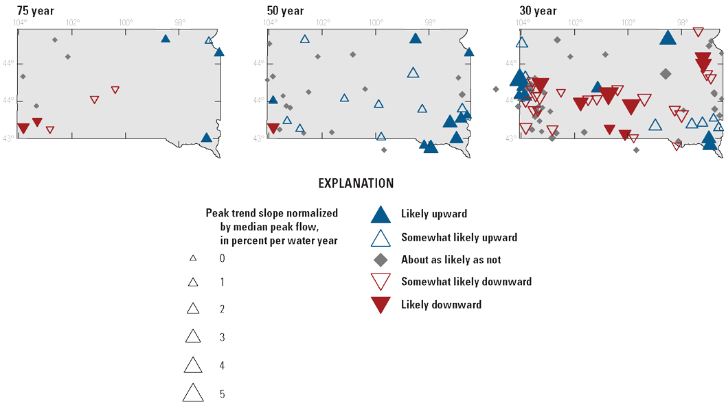
Maps showing likelihoods and directions of monotonic trends in peak-streamflow magnitude in South Dakota for three trend periods (modified from fig. 15 of Barth and Sando [2024]).
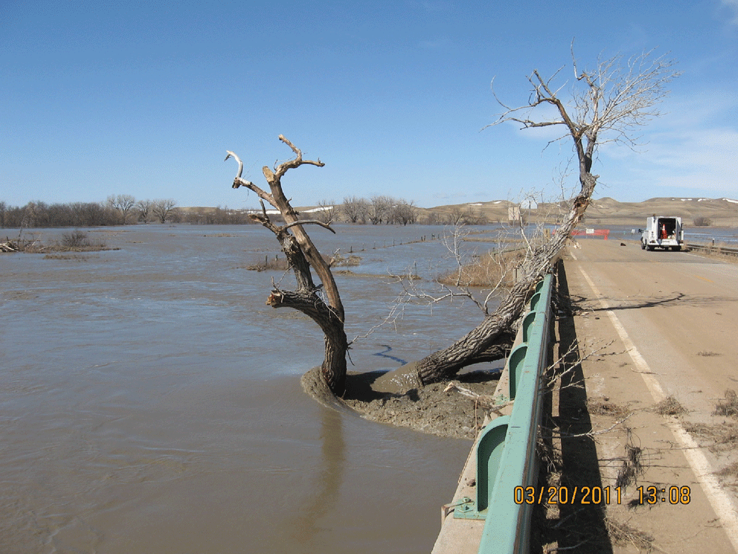
Photograph showing flood conditions on the Moreau River near Whitehorse, South Dakota (U.S. Geological Survey streamgage 06360500), on March 20, 2011. Streamflow for this site set a new peak of record high of 34,200 cubic feet per second. Photograph by Joel Petersen, U.S. Geological Survey.
Detected trends in the annual climate metrics for the 75- and 50-year trend periods indicate a spatially consistent statewide increase in precipitation, decrease in snowfall, increase in potential evapotranspiration, and increase in soil moisture storage (Barth and Sando, 2024). Furthermore, detected trends in seasonal precipitation in the 75- and 50-year trend periods highlight a pronounced change in precipitation in winter and later into the summer season, especially in the 50-year trend period in the eastern part of the State (Barth and Sando, 2024). Statewide increases in seasonal soil moisture storage were also detected (fig. 32), highlighting year-round increasing flood magnitudes, particularly in the eastern part of the State (Barth and Sando, 2024).
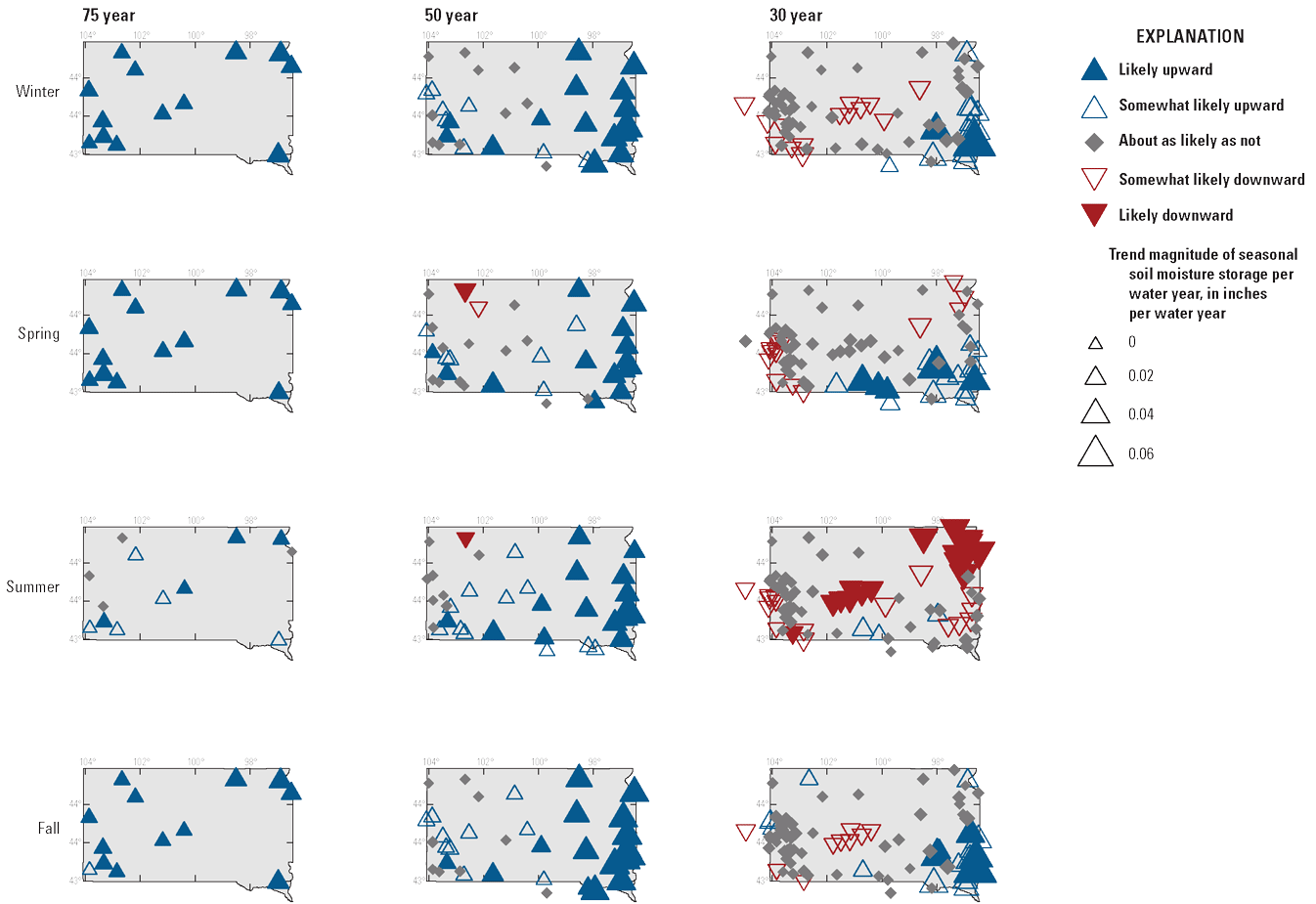
Maps showing likelihoods and magnitudes of trends in seasonal soil moisture storage in study basins in South Dakota for three trend periods and four seasons (winter, December–February; spring, March–May; summer, June–August; and fall, September–November). Symbols are mapped at the outlets of basins (that is, at the location of the streamgage; modified from fig. 36 of Barth and Sando [2024]).
The climate metrics analysis results tended to have more statewide consistency than did the results of peak and daily streamflow analyses. Metrics of streamflow indicated more east-west differences. Several factors contribute to these differences. The combination of increased precipitation in the eastern part of the State, the geologic setting, and related soil composition lead to basin memory, or persistence, in the east. The basin memory also drives changes not only in annual peak and daily streamflow but also in flow durations and volumes (Norton and others, 2022; Barth and Sando, 2024).
Wisconsin Summary
Trends and change points in peak flows varied spatially and temporally during the study period in Wisconsin (Levin, 2024b). Peak flows in the Driftless Area of Wisconsin (a region in the southwestern part of Wisconsin that was not glaciated and is geomorphologically different from other areas of the State with rugged hills and deep, steeply sloped river valleys; refer to fig. 4 of Levin [2024b], also refer to Knox [2019]) decreased from 1920 through the 1980s but increased between 1990 and 2020 (fig. 33). The change in direction of the trend around 1990 was accompanied by a change in the timing of peak flows; peak flows became more common in the late summer and early fall (Levin, 2024b). Peak flows at most streamgages in the southeastern corner of Wisconsin increased throughout all analysis periods (fig. 33). Trends in peak flows in the central and northern regions of Wisconsin were variable, and upward and downward trends were present (fig. 33).
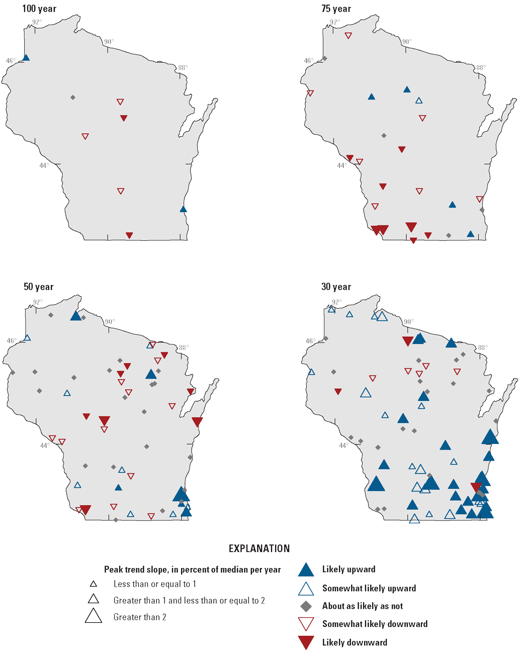
Maps showing likelihoods and magnitudes of monotonic trends in peak-streamflow magnitude in Wisconsin for all trend periods (modified from fig. 10 of Levin [2024b]).
Analyses of daily flows indicated an increase in base flow across all seasons; previously dry fall and winter periods have marked increases in base flow, and the largest increases are in the most recent 30-year period (Levin, 2024b). Temperature increased at most streamgages in the State in the 100-, 75-, and 50- year periods, driven by fall and winter increases. Precipitation also increased at nearly every streamgage, and the largest increases were in the southern part of the State. An example of rainfall-generated flooding in southern Wisconsin is shown in figure 34. Warmer fall and winter temperatures combined with an increase in precipitation are likely driving an increase in overall wetness across the State, leading to larger base flows, increases in peak-streamflow magnitude, and changes in their timing (fig. 35; Levin, 2024b).
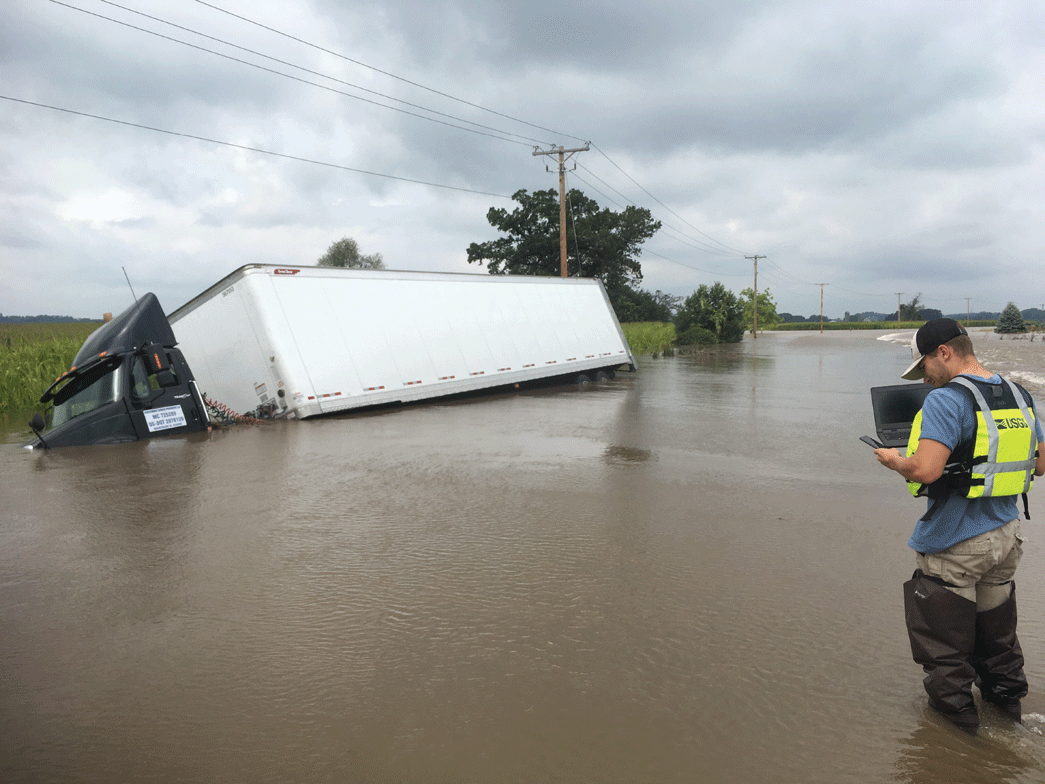
Photograph showing a U.S. Geological Survey hydrologist documenting a flooded street near the Sugar River in Verona, Wisconsin. This photograph was taken after the area received near-record rainfall on August 20, 2018. Photograph by the U.S. Geological Survey.
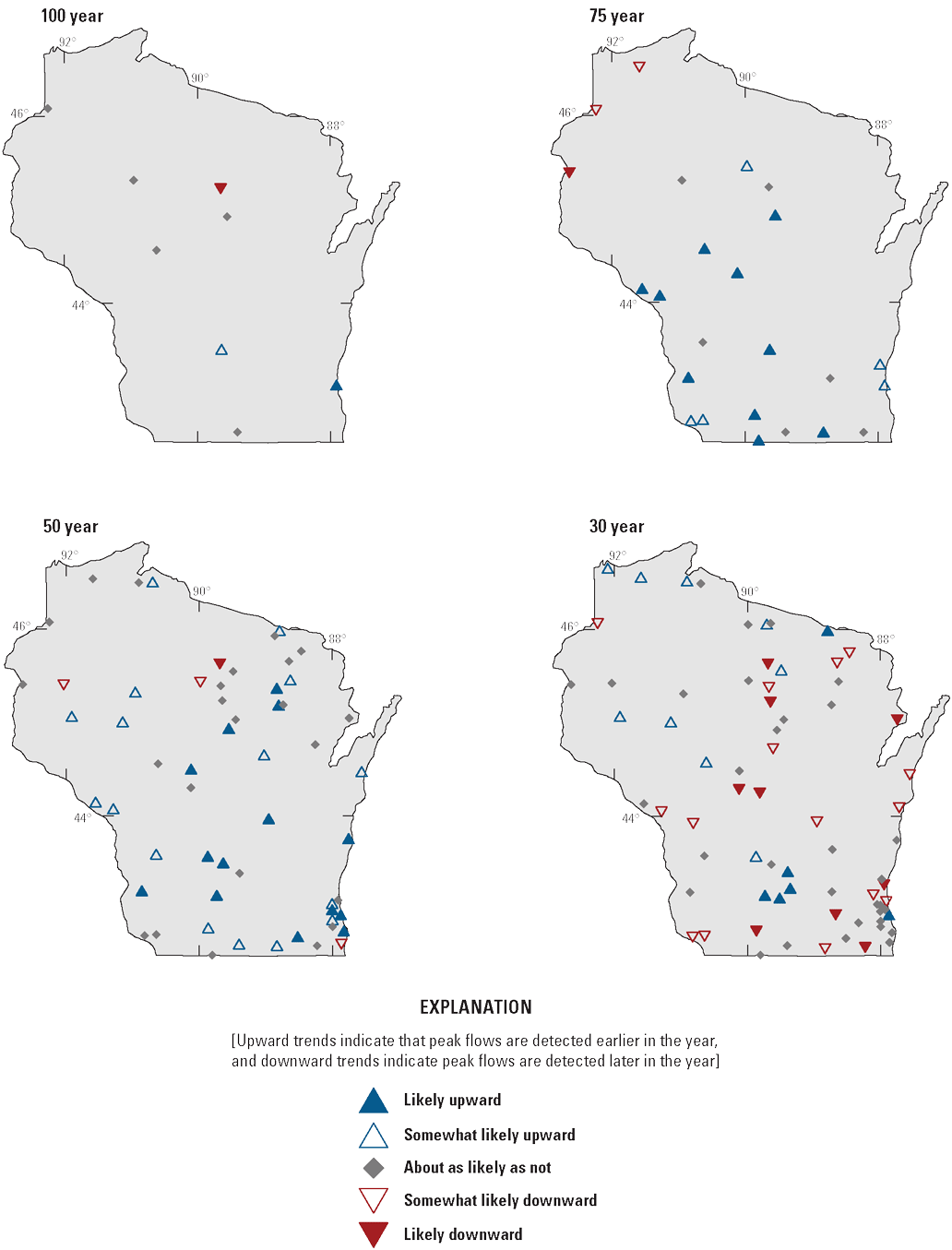
Maps showing likelihoods of peak-streamflow timing trends at selected U.S. Geological Survey streamgages in Wisconsin for four analysis periods ending in water year 2020. Upward trends indicate that peak flow are detected earlier in the year, and downward trends indicate peak streamflows are detected later in the year (modified from fig. 12 of Levin [2024b]). [A water year is the period from October 1 to September 30 and is designated by the year in which it ends]
Seasonality Study
The nine-State hydroclimatic analysis included limited investigation of the timing or seasonality of streamflow (Marti and others, 2024b; Ryberg and others, 2024). As a follow up, a more advanced study was completed using circular statistics to investigate changes in timing and flood-generating mechanisms (Barth and others, 2025). Circular statistics provide a mechanism to analyze the day of the year of an event in a circular fashion, rather than a linear fashion. This circular method is necessary because it allows analysts to accurately represent that January 1 and December 31 are close to each other in time but end up being at opposite ends if a year is represented in a linear fashion.
Circular statistics methods were used to characterize the seasonal properties of annual maximum series (AMS) and partial-duration POT streamflow time series for 841 and 623 selected USGS streamgages, respectively. The streamgages used were those selected for the hydroclimatic variability analyses summarized by State. Therefore, the streamgages analyzed were considered unregulated without substantial diversion. The streamgage selection means that the seasonal patterns were not generated by reservoir operations. In addition, the same 75-, 50-, and 30-year analysis periods through water year 2020 were used (the 100-year analysis period was eliminated because of the small number of sites with records that long). A subset of AMS time series with detected change points (abrupt changes) in the median and (or) spread of the peak flow was analyzed on either side of the change point to evaluate changes in their circular statistics (Barth and others, 2025).
Complete results are available in an associated USGS data release (Barth and others, 2024). Results for the 50-year trend period and implications are summarized here. In the 50-year trend period, five subregions within the nine-State area share common mean flood timing in the AMS and POT partial-duration series (fig. 36). Changes between asymmetric distributions, which tend to have at least two seasons with floods (such as floods generated from snowpack melt and from summer convective storms), and reflective symmetric distributions, which tend to have flood timing concentrated over a number of continuous months (such as floods that are in spring and summer), are detected particularly among the 50- and 30-year trend periods in the States of North Dakota, Minnesota, and Wisconsin. Furthermore, for the subset of streamgages with abrupt change points in the AMS, regional patterns of changes in seasonality are detected between the periods of record before and after the change point. These findings have implications for mixed population analyses; that is, AMS flood-frequency analyses that consider the flood-generating mechanisms. Flood control and response operations also could be affected by changes in high streamflow durations, volumes, and their timing (fig. 37; Barth and others, 2025).
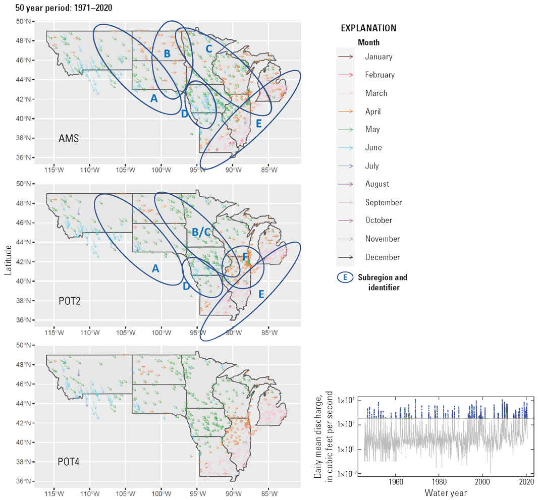
Maps showing the timing (by month, indicated by the color and direction of the arrows, where directionally the months proceed counterclockwise with January upward) and dispersion (indicated by the length of the arrows) for flood peaks from U.S. Geological Survey streamgages in the nine-State study area for the 50-year trend period for the annual maximum series (AMS) and the peaks-over-threshold (POT) partial-duration flood series with an average of two and four daily mean streamflows per water year (POT2 and 4), respectively. A generalized POT2 time series plot is provided to illustrate daily mean values (blue dots) above a POT2 threshold (black horizontal line) (modified from fig. 5 of Barth and others [2025]). [A water year is the period from October 1 to September 30 and is designated by the year in which it ends]
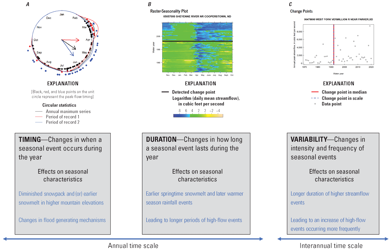
Graphs showing three aspects of seasonality that are affected by climate changes, (A) flood timing, (B) duration, and (C) variability, and examples of their potential effects on seasonal characteristics in the nine-State study area in the north-central United States (modified from fig. 15 of Barth and others [2025]). [A water year is the period from October 1 to September 30 and is designated by the year in which it ends. NR, near; ND, North Dakota; R, River; SD, South Dakota]
Urbanization Study
A relevant land-use change in parts of the study area is urbanization (fig. 38) because of the associated increase in impervious surfaces and the effects on runoff and infiltration. Basins undergoing urbanization often also experience changes in climate, but most previous work on the effect of urbanization on peak flows has considered urbanization alone and only the spatial variation in flood quantiles or its average temporal effect (flood quantiles are the amount of water corresponding to a 100-year flood, a 200-year flood, or some other flood recurrence interval; U.S. Geological Survey, 2024). In addition, most work on the effect of nonstationarity in climate has focused on single-station analyses, which cannot give results for extreme quantiles. To address these gaps, three approaches to the statistical estimation of the joint effects of changes in impervious cover and climate on the estimation of peak-flow quantiles were compared. One method estimates causal effects and peak-flow quantile at individual stations: single-station quantile regression. The other two methods use multiple sites in the same analysis, using panel regression, to add regional information to the model. One method was a fixed effect panel-quantile regression (pQR) method using a location (mean) shift to homogenize the stations in the panel. The other method uses a location-scale panel regression (pQRmom) model, which accounts for location (mean) and scale (variance) effects. The different approaches were applied to a dataset consisting of peak flows from 127 minimally nested basins in Illinois, Iowa, Michigan, Minnesota, Missouri, and Wisconsin with at least a 4-percent change in imperviousness. These data are available in an associated data release (Marti and others, 2024a).
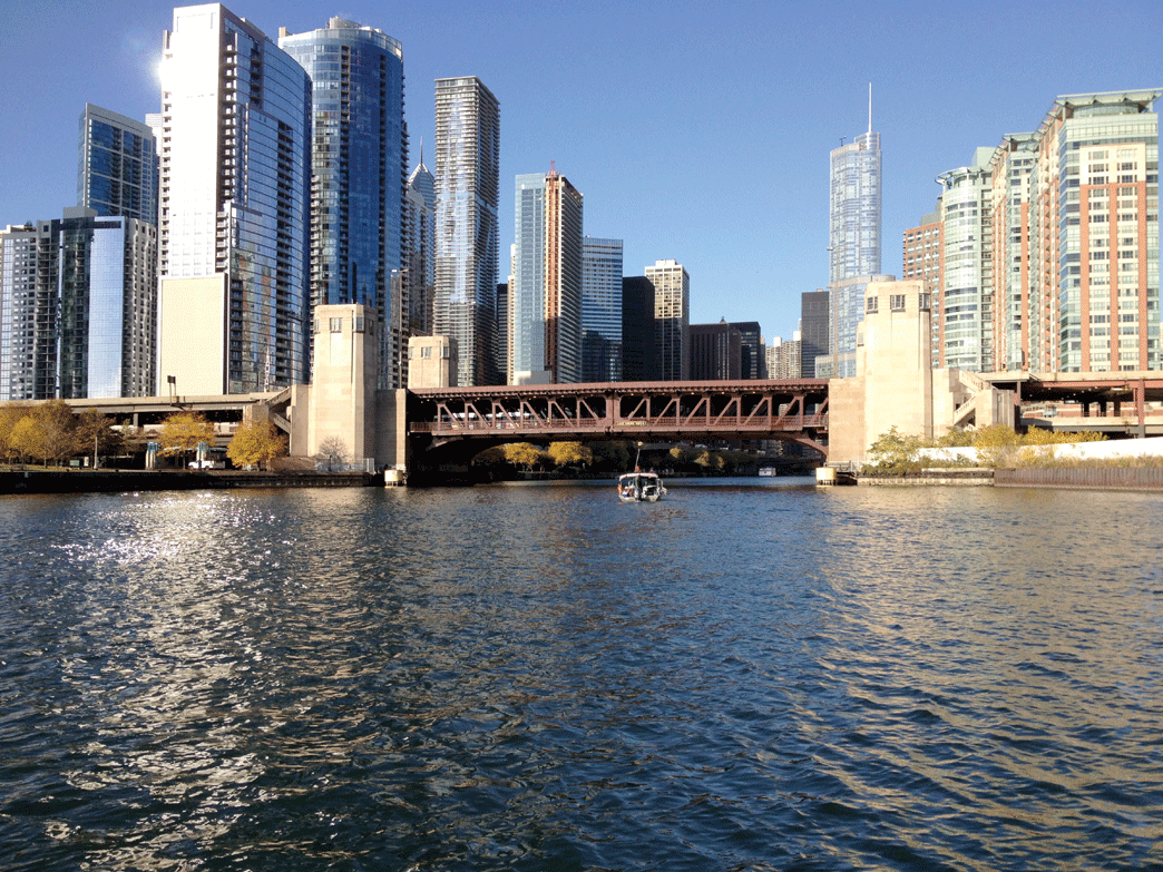
Photograph showing where water and impervious surfaces meet—looking west down the Chicago River main stem from the Chicago River Controlling Works where water enters from Lake Michigan, Illinois. Photograph by Jim Duncker, U.S. Geological Survey.
The annual maximum daily discharge from a water-balance model was selected as the primary climate predictor, although precipitation was also considered. Impervious fraction regression coefficients for the three approaches are shown in figure 39. Single-station regressions were usually effective in determining the effects of climate variation on annual maximum daily discharge but unreliable for determining the effects of urbanization. The panel regression approaches give much more precise results, but their estimates of quantile dependence differ.
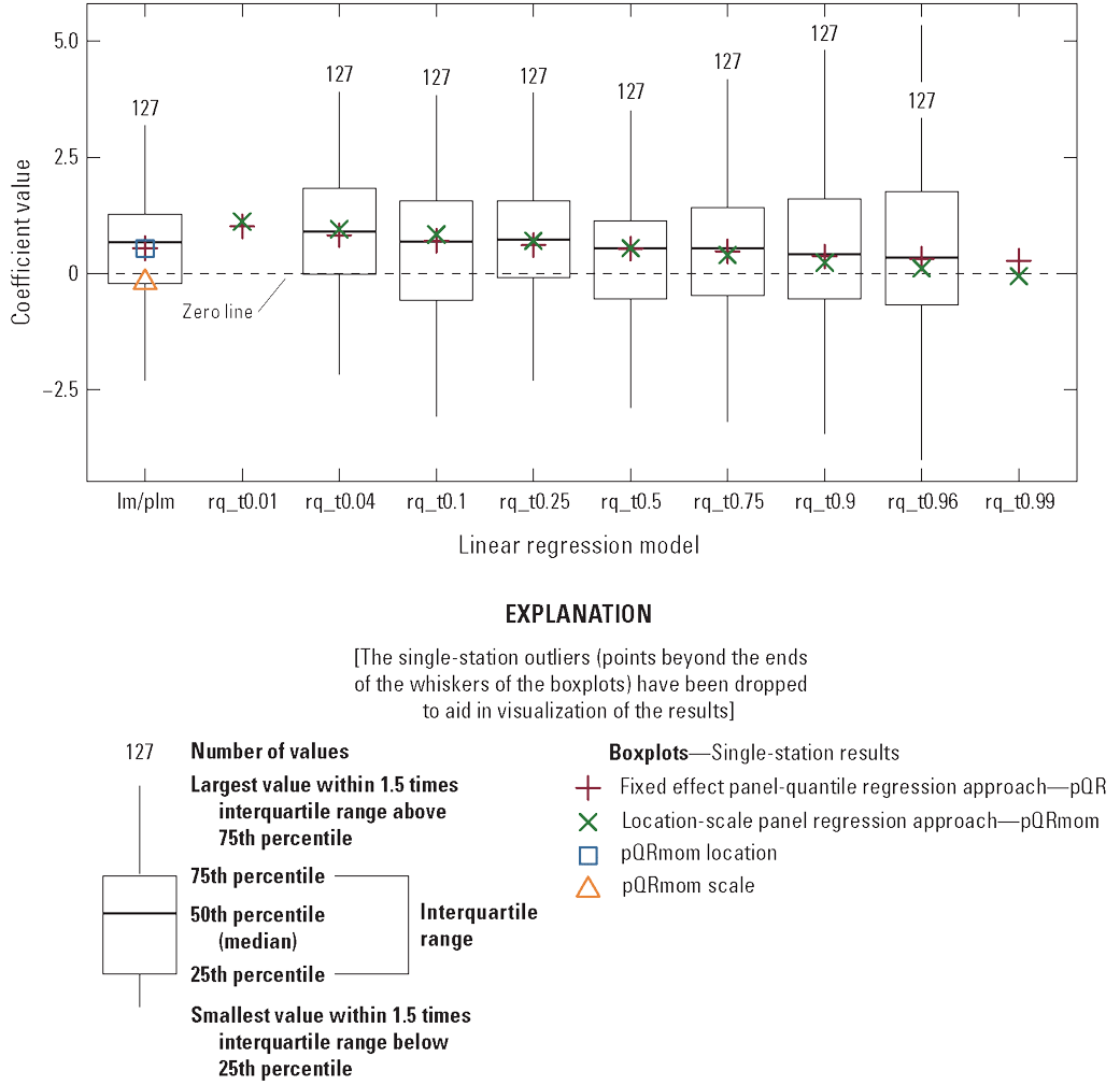
Boxplot showing impervious fraction regression coefficient distributions for the three approaches considered in this study: the single-station quantile regression approach, the fixed effect panel-quantile regression approach, and the location-scale panel regression model (modified from fig. 3B of Over and others [2025]). [lm/plm, single-station and panel least-squares linear model results; rq_tx, quantile regression results for a flood with a nonexceedance probability value from 0.01 to 0.99; pQR, panel-quantile regression approach; pQRmom, location-scale panel regression approach]
Differences in the panel regression methods can be understood by considering at the significance of the urbanization coefficient at different annual exceedance probabilities (AEPs). The AEP is the probability of flooding in any given year considering the full range of possible annual floods (England and others, 2018). An AEP of 0.01, for example, indicates a 1 in 100, or 1 percent, chance of flooding each year. Both methods (pQR and pQRmom) indicate that the larger the flood, the less urbanization affects the magnitude, but they differ in the magnitude at which the urbanization effect becomes insignificant. The pQRmom urbanization coefficients are not significantly different from zero for AEPs less than 0.10, whereas the pQR coefficients remain positive and are significant except for AEP=0.01, the smallest AEP value considered. That is, the pQRmom method determines the urbanization effect goes to zero at floods with less than a 10-percent occurrence each year, but the pQR method determines the urbanization effect goes to zero at larger magnitudes (Over and others, 2025).
Although the location-scale structure of the pQRmom approach has less flexible quantile dependence than the pQR approach, the pQRmom approach has somewhat lower overall error. Results also indicate that by subsetting the dataset to homogenize the scale effects, the pQR and pQRmom results become similar, indicating the insignificant urbanization coefficients for small AEPs of the pQRmom results are likely correct for the study dataset (Over and others, 2025). These findings highlight how selection of the methodology and consideration of variations with AEP can affect results when investigating the joint effects of climate and land use on flooding.
Tile Drainage Study
Subsurface agricultural drainage, also known as tile drainage, uses systems of underground drains that remove excess water from the subsurface to increase agricultural productivity (fig. 40A, B). Subsurface drainage has a complex relation to streamflow characteristics and has been hypothesized as a potential driver of changes in peak flow (Barth and others, 2022). Because of the complex interactions among subsurface drains, precipitation, local soil conditions, and land management practices, subsurface drainage effect on downstream flow has the potential to vary seasonally and by storm events, and not all subsurface drainage systems are expected to have the same effects (Podzorski and Ryberg, 2025). The purpose of this work was to provide a conceptual framework for understanding how peak flow might be affected by tile drainage. Hypotheses presented in this conceptual framework could be tested in future research.
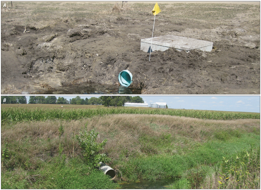
Photographs showing subsurface agricultural tile drainage outlets (A) near Embden, North Dakota, and (B) in the Midwestern Corn Belt. Photographs by (A) Kathleen Rowland and (B) Peter Van Metre, U.S. Geological Survey.
Subsurface drainage can affect the magnitude of peak flow by converting surface runoff from a storm event to subsurface runoff and can differ at the catchment scale compared to the field scale. By increasing hydrologic connectivity of a catchment, subsurface drainage can increase nonevent flow or the streamflow between storm events, which is typically dependent on lateral flow through the subsurface and groundwater. By diverting water from groundwater recharge or by reducing water available for evapotranspiration, subsurface drainage may increase the total volume of streamflow. Finally, changes in precipitation amount, frequency, and timing affect the need for and performance of subsurface drainage.
States in this study area are projected to have increases in precipitation extremes (Knapp and others, 2023; Wilson and others, 2023). These precipitation changes may result in the expanded use of subsurface drainage (estimated tile drainage in 2017 is shown in fig. 41). In addition, changes in precipitation characteristics may increase infiltration excess overland flow, which is also called Hortonian overland flow and is anywhere that surface water input exceeds the infiltration capacity of the surface (Horton, 1933; Tarboton, 2003). Increased infiltration excess overland flow increases flood risk regardless of the presence or absence of subsurface drainage (Podzorski and Ryberg, 2025).
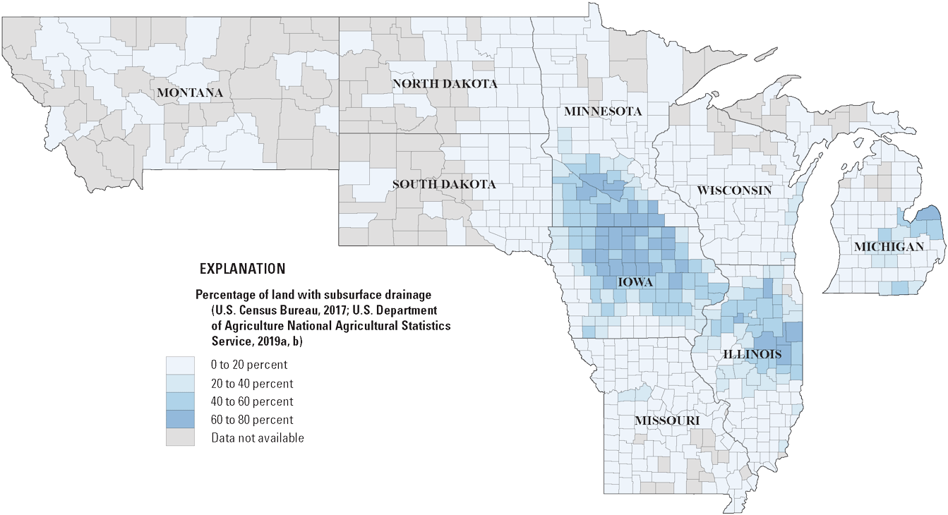
Map showing the percentage of land by county with subsurface agricultural drainage in the nine-State study region (U.S. Census Bureau, 2017; U.S. Department of Agriculture National Agricultural Statistics Service, 2019a, b; modified from fig. 1 of Podzorski and Ryberg [2025]).
Summary of Results and Drivers of Change
In Illinois and Missouri, increases in peak flow are linked to rising annual and seasonal precipitation, despite rising temperatures that increase potential evapotranspiration (Marti and Heimann, 2024; Marti and Over, 2024). In Iowa, trends in precipitation, especially in spring and summer, correspond to peak-flow trends, despite some downward trends in southwestern Iowa (O’Shea, 2024). Iowa has also had changes in seasonality, indicating a shift away from springtime snowmelt driven floods and toward short but intense precipitation-driven flooding (O’Shea, 2024). In Michigan, annual precipitation and temperatures have increased, but modeled potential evapotranspiration to precipitation ratios indicate an overall trend toward wetter conditions (Levin, 2024a). In Minnesota, conditions are wetter in the southern areas and drier in the northern areas of the State, but the peak-flow trends pattern was not as distinct because of changes in snowfall and potential evapotranspiration (Williams-Sether and Sanocki, 2025). In Montana and contributing drainage areas in northern Wyoming, changes in precipitation and snowmelt runoff timing are affecting peak-flow patterns (Sando and others, 2025). In eastern North Dakota, increased annual precipitation is affecting peak flow more than temperature is affecting peak flow, resulting in upward trends, while in western North Dakota, changes in precipitation and temperature result in downward trends (Ryberg and Williams-Sether, 2025). In South Dakota, increased precipitation and soil moisture correlate with rising flood magnitudes (Barth and Sando, 2024). In Wisconsin, increased base flow in fall and winter because of higher precipitation and temperatures is leading to overall wetter conditions (Levin, 2024b).
In previous attributional studies, comparable results were detected at unregulated sites. Long-term precipitation and multidecadal climate variability were determined to be contributing factors to changes in peak flow in western parts of this study area (Sando and others, 2022), and short-term precipitation was a factor in eastern parts (Levin and Holtschlag, 2022). The Fifth National Climate Assessment indicates that temporal and spatial variability will continue to be a dominant feature of precipitation and temperature in the Northern Great Plains with increased risk for floods and droughts (Knapp and others, 2023). In the Midwest, rapid transitions between wet and dry precipitation extremes are expected to increase (Wilson and others, 2023).
In parts of the study area, urbanization has increased floods with lower magnitudes and higher AEPs; that is, floods with a higher frequency (Over and others, 2025). In addition, in parts of the study area, tile drainage could have an effect on streamflow. The effects of these human interventions that affect infiltration and runoff are usefully studied jointly with climate because changes in climate, such as increases in extreme precipitation at a rate that exceeds infiltration, affect how hydrologists model runoff processes and attribute change.
Implications for Flood-Frequency Analysis
Nonstationary flood-frequency analysis necessitates detailed exploratory data analysis and additional data and information about climatic, land-use, and other factors (Serinaldi and Kilsby, 2015). The work summarized here provides extensive exploratory analysis for peak flow and daily streamflow and climate data, as well as major land-use factors, setting the stage for informed nonstationary flood-frequency analysis.
No one nonstationary flood-frequency analysis method is likely applicable to all studies. Many of the suggested nonstationary methods are statistically complex, discouraging widespread adoption. One method of addressing nonstationarity is explaining the nonstationary behavior with an explanatory variable (representing climate or land use) and then generating the conditional mean, variance, and skew with which to complete the stationary flood-frequency analysis (Khaliq and others, 2006; Serago and Vogel, 2018). Generalized additive models for location, scale, and shape can also incorporate explanatory variables and provide a flexible framework for modeling nonstationarities because they can model abrupt changes and trends (Villarini and others, 2009a, b; Machado and others, 2015).
The changes in seasonality and extended periods of high flow can indicate that using only the AMS, peak flow, leaves many floods out of the analysis. A POT approach would include multiple floods in some years (and none in others) that are above a particular threshold. The POT approach has been underused mainly because of the challenge of selecting a threshold and a minimum separation time that ensure independent peaks that meet distributional assumptions and provide enough data for estimation of parameters (Khaliq and others, 2006; Pan and others, 2022).
Results of these studies indicate that the patterns in nonstationarity have spatial cohesiveness or temporal cohesiveness, such as the opposing trends in the Dakotas east and west of the 100th meridian. A panel regression model can incorporate explanatory variables that have fixed effects or vary across space and time and therefore could have a regional component (Khaliq and others, 2006; Ferreira and Ghimire, 2012; Over and others, 2016; Blum and others, 2020). Modeling regional components of flood behavior can be particularly useful given short record lengths at some sites (Khaliq and others, 2006).
In conclusion, by providing exploratory analysis of peak flows and land use and climate drivers, this report sets the stage for the development and application of adaptive flood-frequency analysis methodologies that incorporate the effects of climate and land-use changes. In this way, flood risk can be reassessed considering observed and projected trends with implications for water-resource management, infrastructure design, and disaster preparedness across the north-central United States.
Summary
Flood-frequency analysis provides the basis for estimates of flood risk used by water-resource managers for land-use planning, and it informs the design of essential infrastructure such as bridges and culverts. Federal guidelines for flood-frequency analysis do not offer guidance on addressing changing climate and land-use conditions when estimating floods. However, omitting climatic and land-use changes that cause abrupt or gradual changes in flood regimes can result in a poor representation of the true flood risk.
In response to concerns about changing flood regimes, the U.S. Geological Survey, in cooperation with nine State agencies (Illinois Department of Transportation, Iowa Department of Transportation, Michigan Department of Transportation, Minnesota Department of Transportation, Missouri Department of Transportation, Montana Department of Natural Resources and Conservation, North Dakota Department of Water Resources, South Dakota Department of Transportation, and Wisconsin Department of Transportation) began a study to examine variability and change in hydrology and climate and the effects of urbanization and tile drainage on flooding. The first phase of the study summarized how variability and change in hydrology and climate affects the temporal and spatial distributions of peak-flow data at unregulated sites. The analyses of hydrology and climate were reported in a multichapter Scientific Investigations Report, the findings of which are summarized in this U.S. Geological Survey Circular. The second phase examined changes in seasonality and land-use changes related to urbanization and tile drainage. These additional analyses are published separately and are also summarized in this Circular.
In Illinois and Missouri, increases in peak flow are linked to rising annual and seasonal precipitation, despite rising temperatures that increase potential evapotranspiration. In Iowa, trends in precipitation, especially in spring and summer, correspond to peak-flow trends, despite some downward trends in southwestern Iowa. Iowa has also had changes in seasonality, indicating a shift away from springtime snowmelt driven floods and toward short but intense precipitation-driven flooding. In Michigan, annual precipitation and temperatures have increased, but modeled potential evapotranspiration to precipitation ratios indicate an overall trend toward wetter conditions. In Minnesota, conditions are wetter in the southern areas and drier in the northern areas of the State, but the peak-streamflow trends pattern was not as distinct because of changes in snowfall and potential evapotranspiration. In Montana and contributing watersheds in northern Wyoming, changes in precipitation and snowmelt runoff timing are affecting peak-flow patterns. In eastern North Dakota, increased annual precipitation is affecting peak flow more than temperature is affecting peak flow, resulting in upward trends, while in western North Dakota, changes in precipitation and temperature result in downward trends. In South Dakota, increased precipitation and soil moisture correlate with rising flood magnitudes. In Wisconsin, increased base flow in fall and winter because of higher precipitation and temperatures is leading to overall wetter conditions. In parts of the study area, urbanization has increased floods with lower magnitudes; that is, floods with a higher frequency. In addition, in parts of the study area, tile drainage could have an effect on streamflow. These studies provide extensive exploratory analysis of peak flow, daily streamflow, and climate data, setting the stage for advancements in flood-frequency analysis that incorporate the effects of climate and land-use changes.
References Cited
Barth, N.A., Marti, M.K., Baxamusa, S.R., and Wavra, H.N., 2024, Results from investigating changes in streamflow seasonality associated with hydroclimatic variability in the north-central United States among three discrete temporal periods, 1946–2020: U.S. Geological Survey data release, accessed January 3, 2025, at https://doi.org/10.5066/P13PVGFE.
Barth, N.A., Ryberg, K.R., Gregory, A., and Blum, A.G., 2022, Introduction to attribution of monotonic trends and change points in peak streamflow across the conterminous United States using a multiple working hypotheses framework, 1941–2015 and 1966–2015, chap. A of Ryberg, K.R., ed., Attribution of monotonic trends and change points in peak streamflow across the conterminous United States using a multiple working hypotheses framework, 1941–2015 and 1966–2015: U.S. Geological Survey Professional Paper 1869, p. A1–A29, accessed December 27, 2023, at https://doi.org/10.3133/pp1869.
Barth, N.A., and Sando, S.K., 2024, Peak streamflow trends in South Dakota and their relation to changes in climate, water years 1921–2020, chap. I of Ryberg, K.R., comp., Peak streamflow trends and their relation to changes in climate in Illinois, Iowa, Michigan, Minnesota, Missouri, Montana, North Dakota, South Dakota, and Wisconsin: U.S. Geological Survey Scientific Investigations Report 2023–5064, 70 p., accessed December 31, 2024, at https://doi.org/10.3133/sir20235064I.
Barth, N.A., Wavra, H.N., Koebele, A.R., and Sando, S.K., 2025, Changes in streamflow seasonality associated with hydroclimatic variability in the north-central United States among three discrete temporal periods, 1946–2020: Journal of Hydrology—Regional Studies, v. 57, article 102084, 28 p., accessed December 28, 2024, at https://doi.org/10.1016/j.ejrh.2024.102084.
Blum, A.G., Ferraro, P.J., Archfield, S.A., and Ryberg, K.R., 2020, Causal effect of impervious cover on annual flood magnitude for the United States: Geophysical Research Letters, v. 47, no. 5, article e2019GL086480, 10 p., accessed March 5, 2020, at https://doi.org/10.1029/2019GL086480.
Burn, D.H., and Whitfield, P.H., 2023, Climate related changes to flood regimes show an increasing rainfall influence: Journal of Hydrology, v. 617, part C, article 129075, 13 p., accessed January 3, 2025, at https://doi.org/10.1016/j.jhydrol.2023.129075.
Cohn, T.A., and Lins, H.F., 2005, Nature’s style—Naturally trendy: Geophysical Research Letters, v. 32, no. 23, article L23402, 5 p., accessed October 21, 2021, at https://doi.org/10.1029/2005GL024476.
England, J.F., Jr., Cohn, T.A., Faber, B.A., Stedinger, J.R., Thomas, W.O., Jr., Veilleux, A.G., Kiang, J.E., and Mason Jr., R.R., 2018, Guidelines for determining flood flow frequency—Bulletin 17C (ver. 1.1, May 2019): U.S. Geological Survey Techniques and Methods, book 4, chap. B5, 148 p., accessed May 5, 2022, at https://doi.org/10.3133/tm4B5.
Falcone, J., 2011, GAGES-II—Geospatial attributes of gages for evaluating streamflow: U.S. Geological Survey data release, accessed May 5, 2024, at https://doi.org/10.5066/P96CPHOT.
Ferreira, S., and Ghimire, R., 2012, Forest cover, socioeconomics, and reported flood frequency in developing countries: Water Resources Research, v. 48, no. 8, article W08529, 13 p., accessed February 28, 2024, at https://doi.org/10.1029/2011WR011701.
Han, J., Liu, Z., Woods, R., McVicar, T.R., Yang, D., Wang, T., Hou, Y., Guo, Y., Li, C., and Yang, Y., 2024, Streamflow seasonality in a snow-dwindling world: Nature, v. 629, no. 8014, p. 1075–1081, accessed July 10, 2024, at https://doi.org/10.1038/s41586-024-07299-y.
Helsel, D.R., Hirsch, R.M., Ryberg, K.R., Archfield, S.A., and Gilroy, E.J., 2020, Statistical methods in water resources: U.S. Geological Survey Techniques and Methods, book 4, chap. A3, 458 p., accessed September 19, 2023, at https://doi.org/10.3133/tm4A3.
Horton, R.E., 1933, The role of infiltration in the hydrologic cycle: Transactions, American Geophysical Union, v. 14, no. 1, p. 446–460, accessed January 3, 2025, at https://doi.org/10.1029/TR014i001p00446.
Khaliq, M.N., Ouarda, T.B.M.J., Ondo, J.-C., Gachon, P., and Bobée, B., 2006, Frequency analysis of a sequence of dependent and/or non-stationary hydro-meteorological observations—A review: Journal of Hydrology, v. 329, nos. 3–4, p. 534–552, accessed September 14, 2023, at https://doi.org/10.1016/j.jhydrol.2006.03.004.
Knapp, C.N., Kluck, D.R., Guntenspergen, G., Ahlering, M.A., Aimone, N.M., Bamzai-Dodson, A., Basche, A., Byron, R.G., Conroy-Ben, O., Haggerty, M.N., Haigh, T.R., Johnson, C., Mayes Boustead, B., Mueller, N.D., Ott, J.P., Paige, G.B., Ryberg, K.R., Schuurman, G.W., and Tangen, S.G., 2023, Northern Great Plains, chap. 25 of Crimmins, A.R., Avery, C.W., Easterling, D.R., Kunkel, K.E., Stewart, B.C., and Maycock, T.K., eds., Fifth National Climate Assessment: Washington, D.C., U.S. Global Change Research Program, 58 p., accessed December 19, 2023, at https://doi.org/10.7930/NCA5.2023.CH25.
Knox, J.C., 2019, Geology of the Driftless Area, in Carson, E.C., Rawling, J.E., III, Daniels, J.M., and Attig, J.W., eds., The physical geography and geology of the Driftless Area—The career and contributions of James C. Knox: Boulder, Colo., Geological Society of America, p. 1–36. [Also available at https://doi.org/10.1130/2019.2543(01).]
Langbein, W.B., and Iseri, K.T., 1960, General introduction and hydrologic definitions: U.S. Geological Survey Water Supply Paper 1541–A, 29 p., accessed May 5, 2022, at https://doi.org/10.3133/wsp1541A.
Levin, S.B., 2024a, Peak streamflow trends in Michigan and their relation to changes in climate, water years 1921–2020, chap. D of Ryberg, K.R. comp., Peak streamflow trends and their relation to changes in climate in Illinois, Iowa, Michigan, Minnesota, Missouri, Montana, North Dakota, South Dakota, and Wisconsin: U.S. Geological Survey Scientific Investigations Report 2023–5064, 49 p., accessed August 7, 2024, at https://doi.org/10.3133/sir20235064D.
Levin, S.B., 2024b, Peak streamflow trends in Wisconsin and their relation to changes in climate, water years 1921–2020, chap. J of Ryberg, K.R., comp., Peak streamflow trends and their relation to changes in climate in Illinois, Iowa, Michigan, Minnesota, Missouri, Montana, North Dakota, South Dakota, and Wisconsin: U.S. Geological Survey Scientific Investigations Report 2023–5064, 49 p., accessed April 2, 2024, at https://doi.org/10.3133/sir20235064J.
Levin, S.B., and Holtschlag, D.J., 2022, Attribution of monotonic trends and change points in peak streamflow in the Midwest Region of the United States, 1941–2015 and 1966–2015, chap. D of Ryberg, K.R., ed., Attribution of monotonic trends and change points in peak streamflow across the conterminous United States using a multiple working hypotheses framework, 1941–2015 and 1966–2015: U.S. Geological Survey Professional Paper 1869, p. D1–D22, accessed October 3, 2022, at https://doi.org/10.3133/pp1869.
Lins, H.F., and Cohn, T.A., 2011, Stationarity—Wanted dead or alive?: Journal of the American Water Resources Association, v. 47, no. 3, p. 475–480, accessed March 31, 2022, at https://doi.org/10.1111/j.1752-1688.2011.00542.x.
Machado, M.J., Botero, B.A., López, J., Francés, F., Díez-Herrero, A., and Benito, G., 2015, Flood frequency analysis of historical flood data under stationary and non-stationary modelling: Hydrology and Earth System Sciences, v. 19, no. 6, p. 2561–2576, accessed August 1, 2022, at https://doi.org/10.5194/hess-19-2561-2015.
Marti, M.K., and Heimann, D.C., 2024, Peak streamflow trends in Missouri and their relation to changes in climate, water years 1921–2020, chap. F of Ryberg, K.R., comp., Peak streamflow trends and their relation to changes in climate in Illinois, Iowa, Michigan, Minnesota, Missouri, Montana, North Dakota, South Dakota, and Wisconsin: U.S. Geological Survey Scientific Investigations Report 2023–5064, 50 p., accessed August 7, 2024, at https://doi.org/10.3133/sir20235064F.
Marti, M.K., and Over, T.M., 2024, Peak streamflow trends in Illinois and their relation to changes in climate, water years 1921–2020, chap. B of Ryberg, K.R., comp., Peak streamflow trends and their relation to changes in climate in Illinois, Iowa, Michigan, Minnesota, Missouri, Montana, North Dakota, South Dakota, and Wisconsin: U.S. Geological Survey Scientific Investigations Report 2023–5064, 58 p., accessed August 7, 2024, at https://doi.org/10.3133/sir20235064B.
Marti, M.K., Podzorski, H.L., and Over, T.M., 2024a, Data for investigating the joint effect of changes in impervious cover and climate on trends in floods: U.S. Geological Survey data release, accessed January 3, 2025, at https://doi.org/10.5066/P1ZNSQSG.
Marti, M.K., and Ryberg, K.R., 2023, Method for identification of reservoir regulation within U.S. Geological Survey streamgage basins in the Central United States using a decadal dam impact metric: U.S. Geological Survey Open-File Report 2023–1034, 15 p., accessed March 31, 2022, at https://doi.org/10.3133/ofr20231034.
Marti, M.K., Ryberg, K.R., and Levin, S.B., 2023, Flood-frequency analysis in the Midwest—Addressing potential nonstationarity of annual peak-flow records: AASHTO Technical Committee on Hydrology and Hydraulics, no. 22, p. 9–11, accessed July 3, 2023, at https://transportation.org/design/wp-content/uploads/sites/31/2023/04/Hydrolink-Issue-22.pdf.
Marti, M.K., Wavra, H.N., Over, T.M., Ryberg, K.R., Podzorski, H.L., and Chen, Y.R., 2024b, Peak streamflow data, climate data, and results from investigating hydroclimatic trends and climate change effects on peak streamflow in the Central United States, 1921–2020: U.S. Geological Survey data release, accessed January 25, 2024, at https://doi.org/10.5066/P9R71WWZ.
Milly, P.C.D., Betancourt, J., Falkenmark, M., Hirsch, R.M., Kundzewicz, Z.W., Lettenmaier, D.P., and Stouffer, R.J., 2008, Stationarity is dead—Whither water management?: Science, v. 319, no. 5863, p. 573–574, accessed October 19, 2021, at https://doi.org/10.1126/science.1151915.
Neri, A., Villarini, G., Slater, L.J., and Napolitano, F., 2019, On the statistical attribution of the frequency of flood events across the U.S. Midwest: Advances in Water Resources, v. 127, p. 225–236. [Also available at https://doi.org/10.1016/j.advwatres.2019.03.019.]
Norton, P.A., Delzer, G.C., Valder, J.F., Tatge, W.S., and Ryberg, K.R., 2022, Assessment of streamflow trends in the eastern Dakotas, water years 1960–2019: Scientific Investigations Report 2022–5055, 11 p., accessed October 3, 2022, at https://doi.org/10.3133/sir20225055.
O’Shea, P.S., 2024, Peak streamflow trends in Iowa and their relation to changes in climate, water years 1921–2020, chap. C of Ryberg, K.R., comp., Peak streamflow trends and their relation to changes in climate in Illinois, Iowa, Michigan, Minnesota, Missouri, Montana, North Dakota, South Dakota, and Wisconsin: U.S. Geological Survey Scientific Investigations Report 2023–5064, 55 p., accessed October 4, 2024, at https://doi.org/10.3133/sir20235064C.
Over, T., Marti, M., Ortiz, J., and Podzorski, H., 2025, The joint effect of changes in urbanization and climate on trends in floods—A comparison of panel and single-station quantile regression approaches: Journal of Hydrology, v. 648, article 132281, 21 p., accessed December 11, 2024, at https://doi.org/10.1016/j.jhydrol.2024.132281.
Over, T.M., Saito, R.J., and Soong, D.T., 2016, Adjusting annual maximum peak discharges at selected stations in northeastern Illinois for changes in land-use conditions: U.S. Geological Survey Scientific Investigations Report 2016–5049, 33 p., accessed December 22, 2020, at https://doi.org/10.3133/sir20165049.
Pan, X., Rahman, A., Haddad, K., and Ouarda, T.B.M.J., 2022, Peaks-over-threshold model in flood frequency analysis—A scoping review: Stochastic Environmental Research and Risk Assessment, v. 36, no. 9, p. 2419–2435, accessed November 9, 2022, at https://doi.org/10.1007/s00477-022-02174-6.
Podzorski, H.L., and Ryberg, K.R., 2025, A framework for understanding the effects of subsurface agricultural drainage on downstream flows: U.S. Geological Survey Scientific Investigations Report 2025–5023, 24 p., accessed April 17, 2025, at https://doi.org/10.3133/sir20255023.
Powell, J.W., 1879, Report on the lands of the arid region of the United States with a more detailed account of the land of Utah with maps: Monograph, 203 p., accessed December 7, 2021, at https://doi.org/10.3133/70039240.
RStudio, 2020, R Markdown: RStudio software release, accessed December 1, 2022, at https://rmarkdown.rstudio.com/.
Ryberg, K.R., ed., 2022, Attribution of monotonic trends and change points in peak streamflow across the conterminous United States using a multiple working hypotheses framework, 1941–2015 and 1966–2015: U.S. Geological Survey Professional Paper 1869, chaps. A–H, [variously paged; 328 p.], accessed October 4, 2022, at https://doi.org/10.3133/pp1869.
Ryberg, K.R., comp., 2024a, Peak streamflow trends and their relation to changes in climate in Illinois, Iowa, Michigan, Minnesota, Missouri, Montana, North Dakota, South Dakota, and Wisconsin: U.S. Geological Survey Scientific Investigations Report 2023–5064, [variously paged], accessed January 25, 2024, at https://doi.org/10.3133/sir20235064.
Ryberg, K.R., 2024b, Why snow is crucial for water supply—And what will happen when it becomes scarce: Nature, v. 629, no. 8014, p. 1013–1014, accessed January 4, 2025, at https://doi.org/10.1038/d41586-024-01239-6.
Ryberg, K.R., Akyüz, F.A., Wiche, G.J., and Lin, W., 2016, Changes in seasonality and timing of peak streamflow in snow and semi-arid climates of the north-central United States, 1910–2012: Hydrological Processes, v. 30, no. 8, p. 1208–1218, accessed February 7, 2022, at https://doi.org/10.1002/hyp.10693.
Ryberg, K.R., Lin, W., and Vecchia, A.V., 2014, Impact of climate variability on runoff in the north-central United States: Journal of Hydrologic Engineering, v. 19, no. 1, p. 148–158, accessed March 29, 2023, at https://doi.org/10.1061/(ASCE)HE.1943-5584.0000775.
Ryberg, K.R., Over, T.M., Levin, S.B., Heimann, D.C., Barth, N.A., Marti, M.K., O’Shea, P.S., Sanocki, C.A., Williams-Sether, T.J., Wavra, H.N., Sando, T.R., Sando, S.K., and Liu, M.S., 2024, Introduction and methods of analysis for peak streamflow trends and their relation to changes in climate in Illinois, Iowa, Michigan, Minnesota, Missouri, Montana, North Dakota, South Dakota, and Wisconsin, chap. A of Ryberg, K.R., comp., Peak streamflow trends and their relation to changes in climate in Illinois, Iowa, Michigan, Minnesota, Missouri, Montana, North Dakota, South Dakota, and Wisconsin: U.S. Geological Survey Scientific Investigations Report 2023–5064, 27 p., accessed January 25, 2024, at https://doi.org/10.3133/sir20235064A.
Ryberg, K.R., and Williams-Sether, T., 2025, Peak streamflow trends in North Dakota and their relation to changes in climate, water years 1921–2020, chap. H of Ryberg, K.R., comp., Peak streamflow trends and their relation to changes in climate in Illinois, Iowa, Michigan, Minnesota, Missouri, Montana, North Dakota, South Dakota, and Wisconsin: U.S. Geological Survey Scientific Investigations Report 2023–5064, 80 p., accessed March 4, 2025, at https://doi.org/10.3133/sir20235064H.
Sando, R., Sando, S.K., McCarthy, P.M., and Dutton, D.M., 2016, Methods for estimating peak-flow frequencies at ungaged sites in Montana based on data through water year 2011 (ver. 1.1, February 2018): U.S. Geological Survey Scientific Investigations Report 2015–5019–F, 30 p., accessed October 3, 2022, at https://doi.org/10.3133/sir20155019F.
Sando, R., Sando, S.K., Ryberg, K.R., and Chase, K.J., 2022, Attribution of monotonic trends and change points in peak streamflow in the Upper Plains region of the United States, 1941–2015 and 1966–2015, chap. C, of Ryberg, K.R., ed., Attribution of monotonic trends and change points in peak streamflow across the conterminous United States using a multiple working hypotheses framework, 1941–2015 and 1966–2015: U.S. Geological Survey Professional Paper 1869, p. C1–C36, accessed October 3, 2022, at https://doi.org/10.3133/pp1869.
Sando, S.K., Sando, R.R., Barth, N.A., and Chase, K.J., 2025, Peak streamflow trends in Montana and northern Wyoming and their relation to changes in climate, water years 1921–2020, chap. G of Ryberg, K.R., comp., Peak streamflow trends and their relation to changes in climate in Illinois, Iowa, Michigan, Minnesota, Missouri, Montana, North Dakota, South Dakota, and Wisconsin: U.S. Geological Survey Scientific Investigations Report 2023–5064, 129 p., accessed May 19, 2025, at https://doi.org/10.3133/sir20235064G.
Serago, J.M., and Vogel, R.M., 2018, Parsimonious nonstationary flood frequency analysis: Advances in Water Resources, v. 112, p. 1–16, accessed July 28, 2022, at https://doi.org/10.1016/j.advwatres.2017.11.026.
Serinaldi, F., and Kilsby, C.G., 2015, Stationarity is undead—Uncertainty dominates the distribution of extremes: Advances in Water Resources, v. 77, p. 17–36, accessed December 22, 2020, at https://doi.org/10.1016/j.advwatres.2014.12.013.
Stedinger, J.R., and Griffis, V.W., 2011, Getting from here to where? Flood frequency analysis and climate: Journal of the American Water Resources Association, v. 47, no. 3, p. 506–513, accessed March 31, 2022, at https://doi.org/10.1111/j.1752-1688.2011.00545.x.
Tarboton, D.G., 2003, Runoff generation mechanisms, chap. 2 of Rainfall-runoff processes: Logan, Utah, Utah State University, 159 p., accessed December 23, 2023, at https://hydrology.usu.edu/rrp/.
U.S. Census Bureau, 2017, Cartographic boundary files—Shapefile: U.S. Census Bureau digital data, accessed June 13, 2023, at https://www.census.gov/geographies/mapping-files/time-series/geo/carto-boundary-file.2017.html#list-tab-1556094155.
U.S. Department of Agriculture National Agricultural Statistics Service, 2019a, 2017 Census of Agriculture: U.S. Department of Agriculture National Agricultural Statistics Service, United States Summary and State Data, v. 1, Geographic Area Series part 51, no. AC–17–A–51, accessed September 6, 2023, at https://www.nass.usda.gov/Publications/AgCensus/2017/Full_Report/Volume_1,_Chapter_1_US/usv1.pdf.
U.S. Department of Agriculture National Agricultural Statistics Service, [2019b], Quick Stats: U.S. Department of Agriculture National Agricultural Statistics Service digital data, accessed June 13, 2023, at https://quickstats.nass.usda.gov/.
U.S. Geological Survey, 2021, USGS water data for the Nation: U.S. Geological Survey National Water Information System database, accessed May 23, 2022, at https://doi.org/10.5066/F7P55KJN.
U.S. Geological Survey, 2024, Why do the values for the 100-year flood seem to change with every flood?: U.S. Geological Survey web page, accessed September 18, 2024, at https://www.usgs.gov/faqs/why-do-values-100-year-flood-seem-change-every-flood.
Villarini, G., Serinaldi, F., Smith, J.A., and Krajewski, W.F., 2009a, On the stationarity of annual flood peaks in the continental United States during the 20th century: Water Resources Research, v. 45, no. 8, 17 p., accessed December 22, 2020, at https://doi.org/10.1029/2008WR007645.
Villarini, G., Smith, J.A., Serinaldi, F., Bales, J., Bates, P.D., and Krajewski, W.F., 2009b, Flood frequency analysis for nonstationary annual peak records in an urban drainage basin: Advances in Water Resources, v. 32, no. 8, p. 1255–1266, accessed February 28, 2024, at https://doi.org/10.1016/j.advwatres.2009.05.003.
Vose, R.S., Applequist, S., Squires, M., Durre, I., Menne, M.J., Williams, C.N., Fenimore, C., Gleason, K., and Arndt, D., 2015, NOAA Monthly U.S. Climate Gridded Dataset (NClimGrid) (ver. 1)—Gridded 5km GHCN-daily temperature and precipitation dataset: National Oceanic and Atmospheric Administration National Centers for Environmental Information digital data, accessed January 8, 2021, at https://data.nodc.noaa.gov/cgi-bin/iso?id=gov.noaa.ncdc:C00332.
Wendland, W.M., 1987, Hydroclimatology, in Climatology: Dordrecht, Kluwer Academic Publishers, p. 497–502. [Also available at https://doi.org/10.1007/0-387-30749-4_90.]
Whipple, A.A., Viers, J.H., and Dahlke, H.E., 2017, Flood regime typology for floodplain ecosystem management as applied to the unregulated Cosumnes River of California, United States: Ecohydrology, v. 10, no. 5, article e1817, 18 p., accessed January 3, 2025, at https://doi.org/10.1002/eco.1817.
Wieczorek, M.E., Signell, R.P., McCabe, G.J., and Wolock, D.M., 2022, USGS monthly water balance model inputs and outputs for the conterminous United States, 1895–2020, based on ClimGrid data: U.S. Geological Survey data release, accessed April 26, 2022, at https://doi.org/10.5066/P9JTV1T6.
Williams-Sether, T., and Sanocki, C.A., 2025, Peak streamflow trends in Minnesota and their relation to changes in climate, water years 1921–2020, chap. E of Ryberg, K.R., comp., Peak streamflow trends and their relation to changes in climate in Illinois, Iowa, Michigan, Minnesota, Missouri, Montana, North Dakota, South Dakota, and Wisconsin: U.S. Geological Survey Scientific Investigations Report 2023–5064, 55 p., accessed March 4, 2025, at https://doi.org/10.3133/sir20235064E.
Wilson, A.B., Baker, J.M., Ainsworth, E.A., Andresen, J., Austin, J.A., Dukes, J.S., Gibbons, E., Hoppe, B.O., LeDee, O.E., Noel, J., Roop, H.A., Smith, S.A., Todey, D.P., Wolf, R., and Wood, J.D., 2023, Midwest, chap. 24 of Crimmins, A.R., Avery, C.W., Easterling, D.R., Kunkel, K.E., Stewart, B.C., and Maycock, T.K. eds., Fifth National Climate Assessment: Washington, D.C., U.S. Global Change Research Program, 58 p., accessed December 29, 2023, at https://doi.org/10.7930/NCA5.2023.CH24.
Supplemental Information
A water year is the 12-month period from October 1 through September 30 of the following year and is designated by the calendar year in which it ends.
For more information about this publication, contact:
Director, USGS Dakota Water Science Center
821 East Interstate Avenue, Bismarck, ND 58503
1608 Mountain View Road, Rapid City, SD 57702
605–394–3200
For additional information, visit: https://www.usgs.gov/centers/dakota-water
Publishing support provided by the
Rolla Publishing Service Center
Disclaimers
Any use of trade, firm, or product names is for descriptive purposes only and does not imply endorsement by the U.S. Government.
Although this information product, for the most part, is in the public domain, it also may contain copyrighted materials as noted in the text. Permission to reproduce copyrighted items must be secured from the copyright owner.
Suggested Citation
Ryberg, K.R., Marti, M.K., Barth, N.A., Over, T.M., Levin, S.B., Podzorski, H.L., Sando, S.K., Williams-Sether, T., O’Shea, P.S., and Chase, K.J., 2025, Hydroclimatic and land-use factors affecting peak streamflow in Illinois, Iowa, Michigan, Minnesota, Missouri, Montana, North Dakota, South Dakota, and Wisconsin: U.S. Geological Survey Circular 1557, 56 p., https://doi.org/10.3133/cir1557.
ISSN: 2330-5703 (online)
Study Area
| Publication type | Report |
|---|---|
| Publication Subtype | USGS Numbered Series |
| Title | Hydroclimatic and land-use factors affecting peak streamflow in Illinois, Iowa, Michigan, Minnesota, Missouri, Montana, North Dakota, South Dakota, and Wisconsin |
| Series title | Circular |
| Series number | 1557 |
| DOI | 10.3133/cir1557 |
| Publication Date | July 30, 2025 |
| Year Published | 2025 |
| Language | English |
| Publisher | U.S. Geological Survey |
| Publisher location | Reston, VA |
| Contributing office(s) | Wyoming-Montana Water Science Center, Dakota Water Science Center, Central Midwest Water Science Center, Upper Midwest Water Science Center |
| Description | Report: viii, 56 p.; 3 Data Releases; Dataset |
| Country | United States |
| State | Illinois, Iowa, Michigan, Minnesota, Missouri, Montana, North Dakota, South Dakota, Wisconsin |
| Online Only (Y/N) | Y |
| Additional Online Files (Y/N) | N |