

Forecasting Storm-Induced Coastal Flooding for 21st Century Sea-Level Rise Scenarios in the Hawaiian, Mariana, and American Samoan Islands
Links
- Document: Report (4 MB pdf) , HTML , XML
- Data Release: USGS Data Release - Projected coastal flooding extents and depths for 1-, 20-, and 100-year return interval storms and 0.00, +0.25, +0.50, +1.00, +1.50, +2.00, and +3.00 meter sea-level rise scenarios in the Hawaiian, Mariana, and American Samoan Islands
- NGMDB Index Pages:
- Download citation as: RIS | Dublin Core
Abstract
Oceanographic, coastal engineering, ecologic, and geospatial data and tools were combined to evaluate the increased risks of storm-induced coastal flooding in the populated Hawaiian, Mariana, and American Samoan Islands as a result of climate change and sea-level rise. We followed a hybrid (dynamical and statistical) downscaling approach to map flooding due to waves and storm surge at 10-square meter resolution along all 1,870 kilometers of these islands’ coastlines for annual (1-year), 20-year, and 100-year return-interval storm events and +0.00 meter (m), +0.25 m, +0.50 m, +1.00 m, +1.50 m, +2.00 m, and +3.00 m sea-level rise scenarios. We quantified the coastal flood depths and extents using the latest climate forcing from Intergovernmental Panel for Climate Change’s Sixth Assessment Report Coupled Model Intercomparison Project. The data generated using these methods provide stakeholders and decision makers with a spatially explicit, rigorous valuation of how, where, and when climate change and sea-level rise increase coastal storm-induced flooding to help identify areas where management and (or) restoration could potentially help reduce the risk to, and increase the resiliency of, the coastal communities in the populated Hawaiian, Mariana, and American Samoan Islands.
Introduction
Coastal flooding and erosion from extreme weather events affect thousands of vulnerable coastal communities along the world’s tropical oceans’ coastlines. The impacts of coastal flooding are predicted to worsen during this century because of population growth and climate change, per Hallegatte and others (2013) and Hinkel and others (2014). There is an urgent need to develop better risk reduction and adaptation strategies to reduce coastal flooding and associated hazards (Hinkel and others, 2014; U.S. National Research Council, 2014). For example, the U.S. spends, on average, $500 million per year mitigating such coastal hazards (U.S. Global Change Research Program, 2023).
Observations (Vermeer and Rahmstorf, 2009) and projections (Kopp and others, 2014) of sea level show that global sea-level rise by the end of the 21st century could be meters above year 2000 levels. Although the precise rates of sea-level rise are uncertain, the existing models suggest that eustatic sea level will be substantially higher by the end of the century. Sea-level rise will have a profound impact on low-lying coastal areas. Projections indicate that sea level will be higher in the tropics than the global average (Slangen and others, 2014). Even small projected changes in sea level are projected to make coastal flooding much more frequent, especially in the tropics (Vitousek and others, 2017). Furthermore, research indicates that wave energy is increasing globally from climate change (Reguero and others, 2019, Morim and others, 2019).
Islands are further at risk because they have limited space for adapting to the impacts of coastal flooding. To date, most studies that describe future sea-level rise threats generally have used passive bathtub models to simulate sea-level rise flooding of tropical islands (Berkowitz and others, 2012); however, these models do not incorporate the nonlinear interaction between sea-level rise and waves (Quataert and others, 2015; Storlazzi and others, 2018). Additionally, while global climate models (GCMs) have advanced in recent years, their coarse resolutions and inability to represent mesoscale conditions have so far limited their use for identifying future coastal hazards at the local scale (O’Neill and others, 2018). This limitation can be overcome, however, using a global-to-local downscaling approach like the one described here, which allows us to leverage projected future sea-level rise, tides, surge, and waves.
To better understand the role that climate change and sea-level rise may play in increasing the risk to, and decreasing the resilience of, coastal communities in the populated Hawaiian, Mariana, and American Samoan Islands, the U.S. Geological Survey (USGS), the University of California at Santa Cruz, and Deltares used GCM output to force a series of oceanographic and coastal engineering models. The objective of this report is to present the global-to-local downscaling methodology of these models to define coastal flood hazards due to forecasted climate change and sea-level rise. This includes presentation and discussion of (1) the modeling framework, (2) the required model system inputs, and (3) the resultant generation of local-scale coastal flooding hazards. The resulting coastal flood model water depths and spatial extents are available from Alkins and others (2024).
Methodology
Oceanographic, coastal engineering, ecologic, and geospatial data and tools were combined to provide a quantitative valuation of the coastal flooding hazards caused by climate change and sea-level rise to the Hawaiian, Mariana, and American Samoan Islands. The goal of this effort was to identify how, where, and when climate and sea-level rise increase the risk of storm-induced coastal flooding. This study represents the first unique and comprehensive effort to rigorously quantify the increase in coastal hazard risk caused by climate change and sea-level rise across the populated tropical Pacific Ocean islands of the United States, based on high-resolution flooding modeling. The methods follow a sequence of steps derived from Storlazzi and others (2019, 2021) and Reguero and others (2021) that integrate physics-based oceanographic and coastal engineering modeling, along with ecologic and geospatial data and tools, to quantify the role of climate change and sea-level rise in increasing coastal flooding hazards.
Deep-water Waves and Storm Surges
Hindcasted and forecasted deep-water wave data from WaveWatchIII (Tolman 1997, 1999, 2009) simulations forced from four Intergovernmental Panel on Climate Change (IPCC; https://www.ipcc.ch/) Sixth Assessment Report (AR6) Coupled Model Intercomparison Project, Phase 6 (CMIP6; https://wcrp-cmip.org/cmip-phase-6-cmip6/) GCMs were produced for 31 years (2020–2050) by Erikson and others (2022) for the Hawaiian, Mariana, and American Samoan Islands. Similarly, hindcasted and forecasted tide and storm surge data from the Global Tide and Surge Model (GTSM; Verlaan and others, 2015; Muis and others, 2016, 2020) simulations were forced using the same four GCMs for the same 31 years (2020–2050) by Muis and others (2022) for the Hawaiian, Mariana, and American Samoan Islands. The CMIP6 models are from the HighResMIP project (Haarsma and others, 2016) and are used for both the WaveWatchIII and GTSM simulations: GFDL-CM4C192-highresSST (Guo and others, 2018), CMCC-CM2-VHR4 (Scoccimarro and others, 2017), HadGEM3-GC-31-HM_highres-future (Roberts, 2019a), and HadGEM3-GC-31-HM_highresSST-future (Roberts, 2019b). The future simulations (2020–2050) used IPCC-AR6 Shared Socioeconomic Pathway 8.5 (Lee and others, 2021), which results in a year 2100 radiative forcing level similar to the IPCC 5th Assessment Report’s Relative Concentration Pathway 8.5 climate scenario.
Shallow-water Waves
Following the methodology of Camus and others (2011), more than 270,000 hourly data on wave climate parameters were propagated to the nearshore using a hybrid downscaling approach. The offshore wave climate data were synthesized into 999 combinations of sea states (wave height, wave periods, and wave directions) that best represented the range of conditions from the Erikson and others (2022) database. These selected sea states were then propagated to the coast using the physics-based Simulating Waves Nearshore (SWAN) spectral wave model (Booij and others, 1999; Ris and others, 1999; SWAN, 2016), which simulates wave transformations nearshore by solving the spectral action balance equation. Wave propagation around reef-lined islands has been accurately simulated using SWAN (Hoeke and others, 2011; Taebi and Pattiaratchi, 2014; Storlazzi and others, 2015). Standard SWAN settings were used (for example, Hoeke and others, 2011; Storlazzi and others, 2015), except that the directional spectrum was refined to 5-degree bins (72 total) to better simulate refraction and diffraction in and amongst the islands (appendix 1).
To accurately model from the scale of the island groups or large sections of coastline (on the order of tens of kilometers) down to local scales (on the order of hundreds of meters), a series of dynamically downscaled nested, rectilinear grids were used. The coarse (5-kilometer [km] or 1-km resolution) SWAN grids provided spatially varying boundary conditions for finer-scale (1-km or 200-meter [m] resolution) SWAN grids, with the finest resolution (200-m) grids used for the rest of the modeling infrastructure (fig. 1, appendix 2). The bathymetry for the SWAN grids were generated by grid-cell averaging various topobathymetric digital elevation models (appendix 3). The shallow-water wave conditions from 999 sea-state combination simulations in the finest SWAN grids were extracted at 100-m intervals along the coastline, at a water depth of 30 m, and then reconstructed into hourly time series using multidimensional interpolation techniques (Camus and others, 2011).
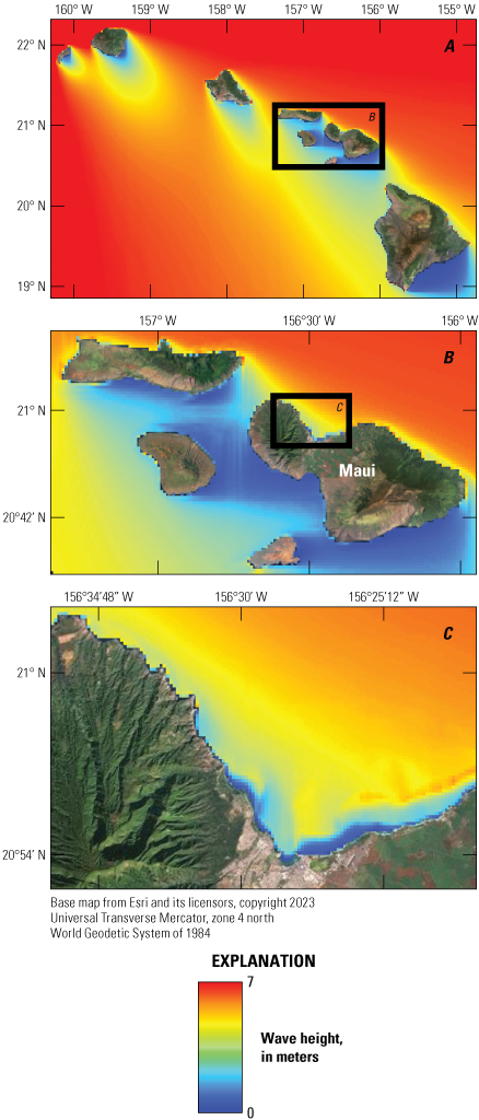
Color maps showing output examples of the Simulating Waves Nearshore (SWAN) model and how 1 of the 999 wave conditions was dynamically downscaled to the 200-meter (m) grid scale offshore West Maui, Hawaiʻi. A, The 5-kilometer (km) resolution Hawaiian Chain model. B, The 1-km resolution Maui Nui model embedded in the Hawaiian Chain model. C, The 200-m resolution West Maui model embedded in the Maui Nui model. Colors indicate significant wave height, in meters.
Benthic habitat maps defining coral reef spatial extent and percent coral cover (appendix 6) were used to delineate the location of nearshore coral reefs and their relative coral abundance along the reef-lined shorelines (fig. 2). Cross-shore transects were created every 100 m alongshore (appendix 4) using the Digital Shoreline Analysis System software version 4.3 in ArcGIS version 10.3 (Thieler and others, 2009). Transects were cast in both landward and seaward directions using the Smoothed Baseline Cast (SBC) method with a 500-m smoothing distance, perpendicular to a baseline generated from coastlines digitized from USGS 1:24,000 quadrangle maps and smoothed in ArcGIS using the Polynomial Approximation with Exponential Kernal algorithm and a 5,000- m smoothing tolerance. Transects had a cross-shore resolution of 1 m and varied in absolute length to ensure each intersected the −30 m and +20 m elevation contours relative to mean sea level. The bathymetric (appendix 3) and coral cover (appendix 6) data were extracted along these shore-normal transects and assigned to the closest transect grid cells.
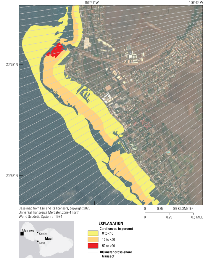
Map showing the coral extent and coverage offshore Lahaina, Maui, Hawaiʻi (Anderson, 2007). Colors indicate percentage of coral coverage; gray lines show cross-shore transects at 100-meter (m) intervals.
The nearshore wave time series (hourly data from 2020 to 2050) at the 30-m isobath were fit to a general extreme value distribution (Méndez and others, 2006; Menéndez and Woodworth, 2010) to obtain the significant wave heights associated with the annual (1-year), 20-year, and 100-year storm return periods in the SWAN grid cells at the end (or nearest the end) of each transect. The corresponding annual (1-year), 20-year, and 100-year storm return period tide and storm surge water levels for the location were taken from the nearest GTSM output point nearest to the offshore end of the each transect.
The return value significant wave heights and associated mean peak periods from SWAN were then propagated over the coral reefs with corresponding (static) return value water levels from GTSM along 100-m spaced shore-normal transects (appendix 4) using the numerical model XBeach (Roelvink and others, 2009; XBeach, 2016), as demonstrated in figure 2. XBeach generated forcing wave time series for each modeled storm return period, which were reused as inputs for modeling different sea level rise scenarios under the same return period. XBeach solves for water level variations up to the scale of long (infragravity) waves using the depth-averaged, nonlinear shallow water equations. The forcing is provided by a coupled wave action balance, in which the spatial and temporal variations of wave energy owing to the incident-period wave groups are solved. The radiation stress gradients derived from these variations result in a wave force that is included in the nonlinear shallow water equations and generates long waves and water level setup within the model. Although XBeach was originally derived for gently sloping sandy beaches, with some additional formulations, it has been applied in reef environments (Pomeroy and others, 2012; van Dongeren and others, 2013; Quataert and others, 2015; Storlazzi and others, 2018) and proved to accurately predict the key reef hydrodynamics.
XBeach was run for 9,000 seconds (s) in one-dimensional hydrostatic mode along the cross-shore transects, at a varying resolution between 10 m seawards and 1 m landwards (resolution varies depending on water depth); the runs generally stabilized after 1,500 s (spin-up time) and thus generate good statistics on waves and wave-driven water levels for more than 2.5 hours (appendix 5). The application of a one-dimensional model neglects some of the dynamics that occur on natural reefs and shorelines, such as lateral flow. Thus, the flooding is likely underrepresented around promontories where wave-energy convergence would cause increased wave-driven flooding that is not captured with one-dimensional models. However, it does represent a conservative estimate for infragravity generation and wave runup, as the forcing is shore normal (for example, van Dongeren and others, 2013; Quataert and others, 2015). Moreover, to reduce the overprediction of infragravity wave energy, the short-wave group variance at the boundary was reduced by 45 percent (wbcEvarreduce = 0.55), per de Goede and others (2020). The choice of a one-dimensional model is warranted in this case because the offshore waves (that is, wave propagation modeled with SWAN) were generally near-normal at the offshore end of the XBeach transects.
The additional formulations that incorporate the effect of higher bottom roughness on incident wave decay through the incident wave friction coefficient (fw) and the current and infragravity wave friction coefficient (cf), as outlined by van Dongeren and others (2013), were applied. The friction induced by corals was parameterized based on the spatially varying coral coverage data and results from a metaanalysis of wave-breaking studies over various reef configurations and friction coefficients for the different coral coverages (for example, van Dongeren and others, 2013; Quataert and others, 2015). Coral coverage classes, as established by the benthic habitat maps, were assigned fw and cf (table 1) over the spatial extent of the reef along the profile as defined from the benthic habitat maps (appendix 6). The future wave and storm surge conditions for each storm return interval were then propagated using the XBeach models over the same 100-m spaced shore-normal transects but modified to account for the different sea-level rise scenarios (fig. 3).
Table 1.
Wave and current friction coefficients for different percentages of coral cover as determined from benthic habitat maps following Storlazzi and others (2019, 2021).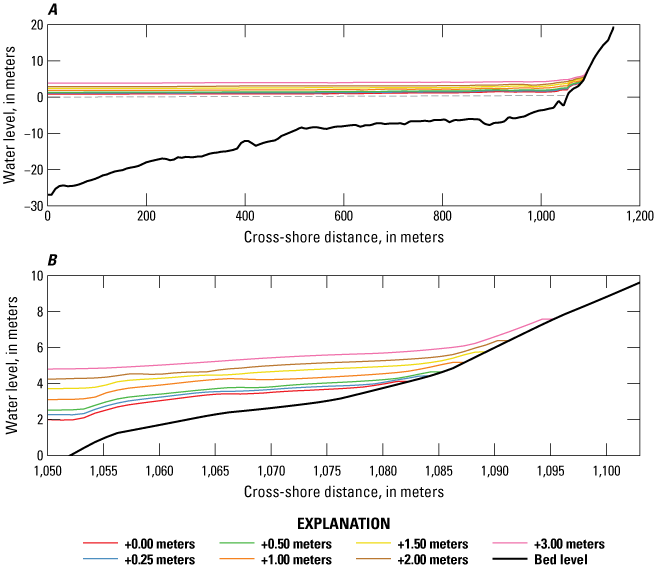
Plots of an example topographic-bathymetric cross section and XBeach model wave-driven total water levels, in meters (m), for the 20-year storm for the seven different sea-level rise scenarios along O’ahu, Hawaiʻi. A, Cross-shore profile 6967 with a continuous fringing reef offshore. B, Zoomed-in view of profile 6967. The black line denotes the seafloor and land, and the colored lines denote the total water level (sea-level rise plus setup plus runup) for the different sea-level rise scenarios.
Coastal Flooding
The Deltares 2-dimensional Super-Fast Inundation of CoastS coastal flooding model (SFINCS) is a super-fast flooding model that dynamically calculates two-dimensional compound flooding maps in coastal areas (Leijnse and others, 2021), which is a vast improvement from interpolating between adjacent XBeach transects per Storlazzi and others (2019). The model uses simplified mass and momentum equations to compute flooding based on water levels and boundary conditions, such as waves, precipitation, and river discharges. Usually, SFINCS ignores the advection term, except for conditions of supercritical flow or when including waves as boundary conditions. In this case, SFINCS was forced with water level and infragravity wave time series; thus, the advection term is included (appendix 7).
The SFINCS boundary conditions were determined from XBeach still water level (tides and surge). The XBeach time series outputs were extracted at the intersection between the transect and the 0.5-m bathymetric contour (below mean sea level), which was below the still water levels during the simulations owing to tides and storm surge; these time series form the basis to force the constant 10-square-meter resolution SFINCS grids (appendix 8), which extended from the 0.5-m bathymetric contour to the 10-m contour. The water level time series boundary conditions were built with a slow ramp-up to avoid initial bathtub-type flooding. The ramp-up goes from mean sea level to the average incoming water level calculated from XBeach. The wave time series were computed as a random signal with a random phase, which were generated from the spectrum calculated from the XBeach incoming water levels (Roelvink and others, 2009; van Dongeren and others, 2013). Both boundary conditions were smoothed in an alongshore direction between adjacent output points to represent a two-dimensional environment. SFINCS was run for 3 hours after the water level ramp-up. A Manning coefficient, which represents friction applied to the flow by the seafloor roughness, of 0.035 was used to account for infragravity wave friction. SFINCS was run for the 3 storm return intervals (fig. 4) and 7 sea-level rise scenarios (fig. 5). SFINCS output flood depth raster data were exported to a geographic information system; the depth rasters were then exported as geotiffs and the flood extent polygons were exported in shapefile format.
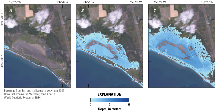
Maps of projected flood depths from the Super-Fast Inundation of CoastS (SFINCS) coastal flooding model at 10-meter resolution for various storm recurrence intervals on south Maui, Hawaiʻi: A, annual (1-year) storm; B, 20-year storm; C, 100-year storm. Colors indicate flood-water depth, in meters. The flood plains for the higher return-period storm scenarios extend farther inland from the shoreline and have greater depths than those for the lower return-period storm scenarios.
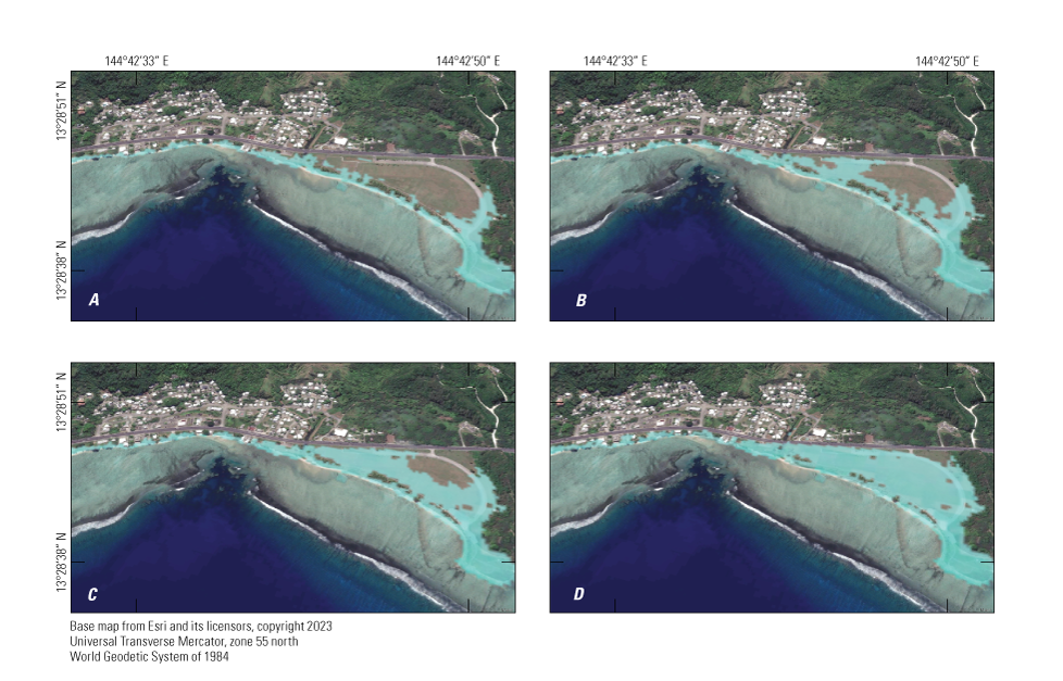
Maps of the projected 20-year storm flood plain extents from the Super-Fast Inundation of CoastS (SFINCS) coastal flooding model at 10-meter (m) resolution for four sea level scenarios at War-in-the-Pacific National Historical Park on west-central Guam: A, current sea level; B, +0.25 m of sea-level rise; C, +0.50 m of sea-level rise; D, +1.00 m of sea-level rise. The flood plains for the higher sea-level rise scenarios extend farther inland from the shoreline than those for the lower sea-level rise scenarios.
Uncertainties, Limitations, and Assumptions
Numerical flood modeling errors were estimated to be ±0.5 m. This value is greater than the root-mean-square and absolute errors computed between model results and measurements (van Dongeren and others, 2013; Quataert and others, 2015) but was used to compensate for the limited number of storms tested and the large geographic scope compared to regions where validation measurements are available. Uncertainties associated with the baseline digital elevation model varied based on input data; see references listed in appendix 3. Other limitations and assumptions pertaining to flood extents include the following:
-
• The extreme value analysis for selecting storm return periods was stationary and did not include nonstationary effects, such as interannual patterns like El Niño, in the selection of values. The fit of each time series had to be limited to several thresholds and could not be adapted iteratively. These thresholds were also different for each region, depending on the local characteristics of extremes in each time series (with a limit of at least 30 extreme values to fit the extreme value distribution).
-
• Because the coral coverage data are defined in five classes, the associated hydrodynamic roughness data are also classified in five classes. This results in a stepwise change in hydrodynamic roughness that can occur over a relatively small distance defining two different coral coverage class polygons that could result from a small change (2 percent; for example, between 9 and 11 percent per table 1) in coral cover.
-
• The model scheme used to define the extreme flood levels were a combination of the wave and surge conditions for certain storm probabilities and did not consider dependencies between both variables or the joint distribution of wave heights, wave periods, and surge levels. However, it is likely that large surges and waves occur simultaneously for large return periods.
-
• We did not separately consider varying tidal levels beyond those registered in the extreme values in the GTSM data that were used to define the extreme sea level for each location.
-
• The modeling structure of one-dimensional nearshore XBeach transects assumes shore-normal wave and wave-driven water level processes.
-
• The same extraction and boundary condition locations were used for all the modeled scenarios. No changes were made for different storms and sea levels.
-
• A constant terrestrial Manning friction value was assumed for the SFINCS models owing to a lack of data for some islands; thus, no differences as a result of land use were considered.
-
• The approach for assessing flood extents associated with each probability assumes that the probability of the extreme flooding conditions on the fore reef defines the probability of the flood zones (thus, the 1-in-100-year total water level represents the 1-in-100-year flood zone).
Conclusions
Here we applied a new methodology to combine oceanographic, coastal engineering, ecologic, and geospatial tools and data to model the impacts of sea-level rise inundation and storm-driven coastal flooding for three storm and seven sea-level rise scenarios. The resulting data make it possible to identify how, when, and where storm-induced flooding hazards will impact the coastal communities in the populated Hawaiian, Mariana, and American Samoan Islands. The goal is to provide sound, scientific guidance for U.S. Federal, State, territorial, commonwealth, and local governments’ efforts on hazard risk reduction and coastal management by providing rigorous, spatially explicit, high-resolution assessments of coastal flooding hazards and, ultimately, to save lives and protect property.
Acknowledgments
This work was carried out by the U.S. Geological Survey (USGS) Coastal and Marine Hazards and Resources Program’s Climate Change Impacts Project as part of an effort in the United States and its trust territories to better understand the effect of climate change and sea-level rise on the U.S. coastlines. This work was supported by U.S. government funding from the Pacific Islands Climate Adaptation Science Center and the USGS Coastal and Marine Hazards and Resources Program. Alex Nereson (USGS) and Kai Parker (USGS) contributed numerous excellent suggestions and a timely review of our work.
References Cited
Alkins, K.C., Gaido L., C., Reguero, B.G., and Storlazzi, C.D., 2024, Projected coastal flooding extents and depths for 1-, 20-, and 100-year return interval storms and 0.00, +0.25, +0.50, +1.00, +1.50, +2.00, and +3.00 meter sea-level rise scenarios in the Hawaiian, Mariana, and American Samoan Islands: U.S. Geological Survey data release, https://doi.org/10.5066/P9RIQ7S7.
Anderson, M., 2007, Benthic habitats of the main eight Hawaiian Islands derived from IKONOS and Quick Bird satellite imagery, 2004–2006: Analytical Laboratories of Hawaii, accessed September 17, 2017, at https://products.coastalscience.noaa.gov/collections/benthic/e97hawaii/data2007.aspx.
Berkowitz, P., Storlazzi, C.D., Courtot, K.N., Krause, C.M., and Reynolds, M.H., 2012, Sea-level rise and wave-driven inundation models for Laysan Island, chap. 2 of Reynolds, M.H., Berkowitz, P., Courtot, K.N., and Krause, C.M., eds., Predicting sea-level rise vulnerability of terrestrial habitat and wildlife of the Northwestern Hawaiian Islands: U.S. Geological Survey Open-File Report 2012–1182, p. 72–126, accessed September 17, 2017, at https://pubs.usgs.gov/of/2012/1182/.
Erikson, L.H., Herdman, L., Flanary, C., Engelstad, A., Pusuluri, P., Barnard, P.L., Storlazzi, C.D., Beck, M., Reguero, B., and Parker, K., 2022, Ocean wave time-series data simulated with a global-scale numerical wave model under the influence of projected CMIP6 wind and sea ice fields: U.S. Geological Survey data release, https://doi.org/10.5066/P9KR0RFM.
Guo, H., John, J.G., Blanton, C., McHugh, C., Nikonov, S., Radhakrishnan, A., Rand, K., Zadeh, N.T., Balaji, V., Durachta, J., Dupuis, C., Menzel, R., Robinson, T., Underwood, S., Vahlenkamp, H., Dunne, K.A., Gauthier, P.P.G., Ginoux, P., Griffies, S.M., Hallberg, R., Harrison, M., Hurlin, W., Lin, P., Malyshev, S., Naik, V., Paulot, F., Paynter, D.J., Ploshay, J., Schwarzkopf, D.M., Seman, C.J., Shao, A., Silvers, L., Wyman, B., Yan, X., Zeng, Y., Adcroft, A., Dunne, J.P., Held, I.M., Krasting, J.P., Horowitz, L.W., Milly, C., Shevliakova, E., Winton, M., Zhao, M., and Zhang, R., 2018, NOAA-GFDL GFDL-CM4 model output prepared for CMIP6 ScenarioMIP ssp585, version 20200501: Earth System Grid Federation web page, accessed September 17, 2022, at https://doi.org/10.22033/ESGF/CMIP6.9268.
Haarsma, R.J., Roberts, M.J., Vidale, P.L., Senior, C.A., Bellucci, A., Bao, Q., Chang, P., Corti, S., Fučkar, N.S., Guemas, V., von Hardenberg, J., Hazeleger, W., Kodama, C., Koenigk, T., Leung, L.R., Lu, J., Luo, J.-J., Mao, J., Mizielinski, M.S., Mizuta, R., Nobre, P., Satoh, M., Scoccimarro, E., Semmler, T., Small, J., and von Storch, J.-S., 2016, High Resolution Model Intercomparison Project (HighResMIP v1.0) for CMIP6: Geoscientific Model Development, v. 9, no. 11, p. 4185–4208, https://doi.org/10.5194/gmd-9-4185-2016.
Hinkel, J., Lincke, D., Vafeidis, A.T., Perrette, M., Nicholls, R.J., Tol, R.S.J., Marzeion, B., Fettweis, X., Ionescu, C., and Levermann, A., 2014, Coastal flood damage and adaptation costs under 21st century sea-level rise: Proceedings of the National Academy of Sciences of the United States of America, v. 111, no. 9, p. 3292–3297, https://doi.org/10.1073/pnas.1222469111.
Kopp, R.E., Horton, R.M., Little, C.M., Mitrovica, J.X., Oppenheimer, M., Rasmussen, D.J., Strauss, B.H., and Tebaldi, C., 2014, Probabilistic 21st and 22nd century sea-level projections at a global network of tide-gauge sites: Earth’s Future, v. 2, no. 8, p. 383–406, https://doi.org/10.1002/2014EF000239.
Lee, J.-Y., Marotzke, J., Bala, G., Cao, L., Corti, S., Dunne, J.P., Engelbrecht, F., Fischer, E., Fyfe, J.C., Jones, C., Maycock, A., Mutemi, J., Ndiaye, O., Panickal, S., and Zhou, T., 2021, Future global climate—Scenario-based projections and near-term information, in Masson-Delmotte, V., Zhai, P., Pirani, A., Connors, S.L., Péan, C., Berger, S., Caud, N., Chen, Y., Goldfarb, L., Gomis, M.I., Huang, M., Leitzell, K., Lonnoy, E., Matthews, J.B.R., Maycock, T.K., Waterfield, T., Yelekçi, O., Yu, R., and Zhou, B., eds., Climate Change 2021, The physical science basis—Contribution of Working Group I to the Sixth Assessment Report of the Intergovernmental Panel on Climate Change: Cambridge, England, and New York, Cambridge University Press, p. 553–672, https://doi.org/10.1017/9781009157896.006.
Leijnse, T., van Ormondt, M., Nederhoff, K., and van Dongeren, A., 2021, Modeling compound flooding in coastal systems using a computationally efficient reduced-physics solver—Including fluvial, pluvial, tidal, wind-and wave-driven processes: Coastal Engineering, v. 163, p. 103796, https://doi.org/10.1016/j.coastaleng.2020.103796.
Morim, J., Hemer, M., Wang, X.L., Cartwright, N., Trenham, C., Semedo, A., Young, I., Bricheno, L., Camus, P., Casas-Prat, M., Erikson, L., Mentaschi, L., Mori, N., Shimura, T., Timmermans, B., Aarnes, O., Breivik, O., Behrens, A., Dobrynin, M., Menendez, M., Staneva, J., Wehner, M., Wolf, J., Kamranzad, B., Webb, A., Stopa, J., and Andutta, F., 2019, Robustness and uncertainties in global multivariate wind-wave climate projections: Nature Climate Change, v. 9, no. 9, p. 711–718, https://doi.org/10.1038/s41558-019-0542-5.
Muis, S., Verlaan, M., Winsemius, H.C., Aerts, J.C.J.H., and Ward, P.J., 2016, A global reanalysis of storm surges and extreme sea levels: Nature Communications, v. 7, article 11969, 11 p., https://doi.org/10.1038/ncomms11969.
Muis, S., Apecechea, M.I., Dullaart, J., de Lima Rego, J., Madsen, K.S., Su, J., Yan, K., and Verlaan, M., 2020, A high-resolution global dataset of extreme sea levels, tides, and storm surges, including future projections: Frontiers in Marine Science, v. 7, p. 263, https://doi.org/10.3389/fmars.2020.00263.
Muis, S., Apecechea, M., Álvarez, J., Verlaan, M., Yan, K., Dullaart, J., Aerts, J., Duong, T., Ranasinghe, R., Erikson, L., O’Neill, A., le Bars, D., Haarsma, R., and Roberts, M., 2022, Global water level change indicators from 1950 to 2050 derived from HighResMIP climate projections: Copernicus Climate Change Service Climate Data Store, accessed October 18, 2022, at https://cds-dev.copernicus-climate.eu/cdsapp#!/dataset/sis-water-level-change-cmip6-indicators?tab=overview.
O’Neill, A.C., Erikson, L.E., Barnard, P.L., Limber, P.W., Vitousek, S., Warrick, J.A., Foxgrover, A.C., and Lovering, J., 2018, Projected 21st century coastal flooding in the Southern California Bight. Part 1—Development of the third generation CoSMoS model: Journal of Marine Science and Engineering, v. 6, no. 2, p. 59, https://doi.org/10.3390/jmse6020059.
Quataert, E., Storlazzi, C.D., van Rooijen, A., Cheriton, O.M., and van Dongeren, A., 2015, The influence of coral reefs and climate change on wave-driven flooding of tropical coastlines: Geophysical Research Letters, v. 42, no. 15, p. 6407–6415, https://doi.org/10.1002/2015GL064861.
Reguero, B.G., Storlazzi, C.D., Gibbs, A.E., Shope, J.B., Cole, A.D., Cumming, K.A., and Beck, M.W., 2021, The value of US coral reefs for flood risk reduction: Nature Sustainability, v. 4, no. 8, p. 688–698, https://doi.org/10.1038/s41893-021-00706-6.
Roberts, M., 2019a, MOHC HadGEM3-GC31-HM model output prepared for CMIP6 HighResMIP highres-future, version 20200501: Earth System Grid Federation web page, accessed September 17, 2022, at https://doi.org/10.22033/ESGF/CMIP6.5984.
Roberts, M., 2019b, MOHC HadGEM3-GC31-HM model output prepared for CMIP6 HighResMIP highresSST-future, version 20200501: Earth System Grid Federation web page, accessed September 17, 2022, at https://doi.org/10.22033/ESGF/CMIP6.6008.
Reguero, B.G., Losada, I.J., and Mendez, F.J., 2019, A recent increase in global wave power as a consequence of oceanic warming: Nature Communications, v. 10, no. 1, p. 205, https://doi.org/10.1038/s41467-018-08066-0.
Scoccimarro, E., Bellucci, A., and Peano, D., 2017, CMCC CMCC-CM2-VHR4 model output prepared for CMIP6 HighResMIP. Version 20200501: Earth System Grid Federation web page, accessed September 17, 2022, at https://doi.org/10.22033/ESGF/CMIP6.1367.
Slangen, A.B.A., Carson, M., Katsman, C.A., van de Wal, R.S.W., Köhl, A., Vermeersen, L.L.A., and Stammer, D., 2014, Projecting twenty-first century regional sea-level changes: Climatic Change, v. 124, no. 1-2, p. 317–332, https://doi.org/10.1007/s10584-014-1080-9.
Storlazzi, C.D., Elias, E.P.L., and Berkowitz, P., 2015, Many atolls may be uninhabitable within decades due to climate change: Scientific Reports, v. 5, no. 1, p. 14546, https://doi.org/10.1038/srep14546.
Storlazzi, C.D., Gingerich, S.B., van Dongeren, A., Cheriton, O.M., Swarzenski, P.W., Quataert, E., Voss, C.I., Field, D.W., Annamalai, H., Piniak, G.A., and McCall, R., 2018, Most atolls will be uninhabitable by the mid-21st century because of sea-level rise exacerbating wave-driven flooding: Science Advances, v. 4, no. 4, eaap9741, https://doi.org/10.1126/sciadv.aap9741.
Storlazzi, C.D., Reguero, B.G., Cole, A.D., Lowe, E., Shope, J.B., Gibbs, A.E., Nickel, B.A., McCall, R.T., van Dongeren, A.R., and Beck, M.W., 2019, Rigorously valuing the role of U.S. coral reefs in coastal hazard risk reduction: U.S. Geological Survey Open-File Report 2019–1027, 42 p., accessed September 17, 2022, at https://doi.org/10.3133/ofr20191027.
Storlazzi, C.D., Reguero, B.G., Cumming, K.A., Cole, A.D., Shope, J.A., Gaido L., C., Viehman, T.S., Nickel, B.A., and Beck, M.W., 2021, Rigorously valuing the coastal hazard risks reduction provided by potential coral reef restoration in Florida and Puerto Rico: U.S. Geological Survey Open-File Report 2021–1054, 35 p., accessed September 17, 2022, at https://doi.org/10.3133/ofr20211054.
SWAN, 2016, SWAN web page, accessed December 19, 2016, at https://www.tudelft.nl/en/ceg/over-faculteit/departments/hydraulic-engineering/sections/environmental-fluid-mechanics/research/swan/.
Taebi, S., and Pattiaratchi, C., 2014, Hydrodynamic response of a fringing coral reef to a rise in mean sea level: Ocean Dynamics, v. 64, no. 7, p. 975–987, https://doi.org/10.1007/s10236-014-0734-5.
Thieler, E.R., Himmelstoss, E.A., Zichichi, J.L., and Ergul, A., 2009, The Digital Shoreline Analysis System (DSAS) version 4.0—An ArcGIS™ extension for calculating shoreline change: U.S. Geological Survey Open-File Report 2008–1278, https://cmgds.marine.usgs.gov/publications/DSAS/of2008-1278/.
U.S. Global Change Research Program, 2023, Coastal erosion: U.S. Climate Resilience Toolkit web page, accessed March 23, 2023, at https://toolkit.climate.gov/topics/coastal-flood-risk/coastal-erosion.
Vitousek, S.K., Barnard, P.L., Fletcher, C.H., Frazer, N., Erikson, L.H., and Storlazzi, C.D., 2017, Doubling of coastal flooding frequency within decades due to sea-level rise: Scientific Reports, v. 7, p. 1399, https://doi.org/10.1038/s41598-017-01362-7.
XBeach, 2016, XBeach Open Source Community:XBeach Open Source Community web page, accessed December 19, 2016, at https://oss.deltares.nl/web/xbeach/.
Appendix 1. SWAN Model Settings
General
	OnlyInputVerify	= false
	SimMode		= stationary
	DirConvention	= nautical
	WindSpeed	= 0.0000000e+000
	WindDir		= 0.0000000e+000
Processes
	GenModePhys	= 3
	Breaking	= true
	BreakAlpha	= 1.0000000e+000
	BreakGamma	= 7.3000002e-001
	Triads		= false
	TriadsAlpha	= 1.0000000e-001
	TriadsBeta	= 2.2000000e+000
	WaveSetup	= false
	BedFriction	= jonswap
	BedFricCoef	= 6.7000002e-002
	Diffraction	= true
	DiffracCoef	= 2.0000000e-001
	DiffracSteps	= 5
	DiffracProp	= true
	WindGrowth	= false
	WhiteCapping	= Komen
	Quadruplets	= false
	Refraction	= true
	FreqShift	= true
	WaveForces	= dissipation 3d
Numerics
	DirSpaceCDD	= 5.0000000e−001
	FreqSpaceCSS	= 5.0000000e−001
	RChHsTm01	= 2.0000000e−002
	RChMeanHs	= 2.0000000e−002
	RChMeanTm01	= 2.0000000e−002
	PercWet		= 9.8000000e+001
	MaxIter		= 100
Output
	TestOutputLevel	= 0
	TraceCalls	= false
	UseHotFile	= false
	WriteCOM	= false
Domain
	DirSpace	= circle
	NDir		= 72
	StartDir	= 0.0000000e+000
	EndDir		= 0.0000000e+000
	FreqMin		= 5.0000001e−002
	FreqMax		= 1.0000000e+000
	NFreq		= 24
	Output		= true
Boundary
	Definition	= orientation
	SpectrumSpec	= parametric
	SpShapeType	= jonswap
	PeriodType	= peak
	DirSpreadType	= power
	PeakEnhanceFac	= 3.3000000e+000
	GaussSpread	= 9.9999998e−003
Appendix 2. SWAN Model Grid Information
Table 2.1.
SWAN model grid sizes, dimensions, and data sources.[km, kilometer; m, meter; NGDC, National Geophysical Data Center; PacIOOS, Pacific Islands Ocean Observing System; —, not applicable]
| Location | 5‑km grid cells | 1‑km grid cells | 200‑m grid cells | Grid dimensions (E‑W × N‑S) | Data source |
|---|---|---|---|---|---|
| American Samoa | — | AmSam | — | 164 × 28 | Lim and others, 2010 |
| American Samoa | — | — | Tutuila | 235 × 100 | Carignan and others, 2013 |
| American Samoa | — | — | Ofu-Olosega & Tau | 155 × 79 | Lim and others, 2010 |
| Northern Mariana Islands | — | — | Saipan | 151 × 136 | PacIOOS, 2016 |
| Guam | — | — | Guam | 221 × 285 | Chamberlin, 2008 |
| Hawai’i | HiChain | — | — | 295 × 192 | NGDC, 2005 |
| Hawai’i | — | Hawaii | — | 142 × 159 | NGDC, 2005 |
| Hawai’i | — | — | Hawaii_North | 400 × 190 | NGDC, 2005 |
| Hawai’i | — | — | Hawaii_East | 235 × 300 | NGDC, 2005 |
| Hawai’i | — | — | Hawaii_Southeast | 310 × 160 | NGDC, 2005 |
| Hawai’i | — | — | Hawaii_South | 350 × 205 | NGDC, 2005 |
| Hawai’i | — | — | Hawaii_West | 185 × 400 | NGDC, 2005 |
| Hawai’i | — | MauiNui | — | 146 × 86 | NGDC, 2005 |
| Hawai’i | — | — | Molokai | 146 × 86 | NGDC, 2005 |
| Hawai’i | — | — | Maui_East | 265 × 220 | NGDC, 2005 |
| Hawai’i | — | — | Maui_West | 195 × 230 | NGDC, 2005 |
| Hawai’i | — | — | Oahu | 420 × 290 | NGDC, 2005 |
| Hawai’i | — | — | Kauai | 293 × 242 | NGDC, 2005 |
References Cited
Carignan, K.S., Eakins, B.W., Love, M.R., Sutherland, M.G., and McLean, S.J., 2013, Tutuila, American Samoa 1/3 arc-second MHW coastal digital elevation model: National Oceanic and Atmospheric Administration, accessed December 19, 2016, at https://www.ngdc.noaa.gov/dem/squareCellGrid/download/4610. [Data moved by time of publication; accessed March 1, 2019, at https://data.noaa.gov//metaview/page?xml=NOAA/NESDIS/NGDC/MGG/DEM/iso/xml/4610.xml&view=getDataView&header=none.]
Chamberlin, C., 2008, Guam 1/3 arc-second MHW coastal digital elevation model: National Oceanic and Atmospheric Administration, accessed December 19, 2016, at https://www.ngdc.noaa.gov/dem/squareCellGrid/download/586. [Data moved by time of publication; accessed March 1, 2019, at https://data.noaa.gov//metaview/page?xml=NOAA/NESDIS/NGDC/MGG/DEM/iso/xml/586.xml&view=getDataView&header=none.]
Lim, E., Taylor, L.A., Eakins, B.W., Carignan, K.S., Grothe, P.R., Caldwell, R.J., and Friday, D.Z., 2010, Pago Pago, American Samoa 3 arc-second MHW coastal digital elevation model: National Oceanic and Atmospheric Administration Technical Memorandum NESDIS NGDC-36, accessed December 19, 2016, at https://www.ngdc.noaa.gov/dem/squareCellGrid/download/647. [Data moved by time of publication; accessed March 1, 2019, at https://data.noaa.gov//metaview/page?xml=NOAA/NESDIS/NGDC/MGG/DEM/iso/xml/647.xml&view=getDataView&header=none.]
National Geophysical Data Center [NGDC], 2005, U.S. Coastal Relief Model vol. 10—Hawaii: National Oceanic and Atmospheric Administration National Geophysical Data Center, accessed December 18, 2016, at https://doi.org/10.7289/V5RF5RZZ.
Pacific Islands Ocean Observing System [PacIOOS], 2016, USGS 10-m digital elevation model, Commonwealth of the Northern Mariana Islands—Saipan: University of Hawaiʻi at Mānoa, accessed December 19, 2016, at http://oos.soest.hawaii.edu/erddap/griddap/usgs_dem_10m_saipan.html.
Appendix 3. Bathymetric Datasets
Table 3.1.
Bathymetric data sources.[NGDC, National Geophysical Data Center; NOAA, National Oceanic and Atmospheric Administration; PacIOOS, Pacific Islands Ocean Observing System; PIBHMC, Pacific Islands Benthic Habitat Mapping Center]
| Location | Sublocation | Data source |
|---|---|---|
| American Samoa | Tutuila | Carignan and others, 2013 |
| American Samoa | Ofu, Olosega, and Taʻū | Lim and others, 2010 |
| Northern Mariana Islands | Saipan Island | PIBHMC, 2007a; Amante and Eakins, 2009; PacIOOS, 2016a |
| Northern Mariana Islands | Tinian Island | PIBHMC, 2007b; Amante and Eakins, 2009; PacIOOS, 2016b |
| Guam | Guam | Chamberlin, 2008 |
| Hawai’i | Island of Hawaiʻi | NGDC, 2005 |
| Hawai’i | Hilo | Love and others, 2011a |
| Hawai’i | Kawaihae | Carignan and others, 2011a |
| Hawai’i | Keauhou | Carignan and others, 2011b |
| Hawai’i | Maui Nui | NGDC, 2005 |
| Hawai’i | Maui | Taylor and others, 2008; NOAA, 2016 |
| Hawai’i | Lānaʻi | NGDC, 2005 |
| Hawai’i | Molokaʻi | NGDC, 2005 |
| Hawai’i | Kahoʻolawe | NGDC, 2005 |
| Hawai’i | Kauaʻi | Friday and others, 2012 |
| Hawai’i | Niʻihau | Friday and others, 2012 |
| Hawai’i | Oʻahu | Love and others, 2011b |
References Cited
Amante, C., and Eakins, B.W., 2009, ETOPO1 1 arc-minute global relief model: National Oceanic and Atmospheric Administration Technical Memorandum NESDIS NGDC-24, accessed on September 1, 2016, at https://doi.org/10.7289/V5C8276M.
Carignan, K.S., Taylor, L.A., Eakins, B.W., Friday, D.Z., Grothe, P.R., Lim, E., and Love, M.R., 2011a, Kawaihae, Hawaii 1/3 arc-second MHW coastal digital elevation model: National Oceanic and Atmospheric Administration, accessed December 19, 2016, at https://www.ngdc.noaa.gov/dem/squareCellGrid/download/1842. [Data moved by time of publication; accessed March 1, 2019, at https://data.noaa.gov//metaview/page?xml=NOAA/NESDIS/NGDC/MGG/DEM/iso/xml/1842.xml&view=getDataView&header=none.]
Carignan, K.S., Taylor, L.A., Eakins, B.W., Friday, D.Z., Grothe, P.R., Lim, E., and Love, M.R., 2011b, Keauhou, Hawaii 1/3 arc-second MHW coastal digital elevation model: National Oceanic and Atmospheric Administration, accessed December 19, 2016, at https://www.ngdc.noaa.gov/dem/squareCellGrid/download/1941. [Data moved by time of publication; accessed March 1, 2019, at https://data.noaa.gov//metaview/page?xml=NOAA/NESDIS/NGDC/MGG/DEM/iso/xml/1941.xml&vvie=getDataView&header=none.]
Carignan, K.S., Eakins, B.W., Love, M.R., Sutherland, M.G., and McLean, S.J., 2013, Tutuila, American Samoa 1/3 arc-second MHW coastal digital elevation model: National Oceanic and Atmospheric Administration, accessed December 19, 2016, at https://www.ngdc.noaa.gov/dem/squareCellGrid/download/4610. [Data moved by time of publication; accessed March 1, 2019, at https://data.noaa.gov//metaview/page?xml=NOAA/NESDIS/NGDC/MGG/DEM/iso/xml/4610.xml&view=getDataView&header=none.]
Chamberlin, C., 2008, Guam 1/3 arc-second MHW coastal digital elevation model: National Oceanic and Atmospheric Administration, accessed December 19, 2016, at https://www.ngdc.noaa.gov/dem/squareCellGrid/download/586. [Data moved by time of publication; accessed March 1, 2019, at https://data.noaa.gov//metaview/page?xml=NOAA/NESDIS/NGDC/MGG/DEM/iso/xml/586.xml&view=getDataView&header=none.]
Friday, D.Z., Taylor, L.A., Eakins, B.W., Carignan, K.S., Love, M.R., and Grothe, P.R., 2012, Kauai, Hawaii 1/3 arc-second MHW coastal digital elevation model: National Oceanic and Atmospheric Administration, accessed December 19, 2016, at https://www.ngdc.noaa.gov/dem/squareCellGrid/download/3550. [Data moved by time of publication; accessed March 1, 2019, at https://data.noaa.gov//metaview/page?xml=NOAA/NESDIS/NGDC/MGG/DEM/iso/xml/3550.xml&view=getDataView&header=none.]
Lim, E., Taylor, L.A., Eakins, B.W., Carignan, K.S., Grothe, P.R., Caldwell, R.J., and Friday, D.Z., 2010, Pago Pago, American Samoa 3 arc-second MHW coastal digital elevation model: National Oceanic and Atmospheric Administration Technical Memorandum NESDIS NGDC-36, accessed December 19, 2016, at https://www.ngdc.noaa.gov/dem/squareCellGrid/download/647. [Data moved by time of publication; accessed March 1, 2019, at https://data.noaa.gov//metaview/page?xml=NOAA/NESDIS/NGDC/MGG/DEM/iso/xml/647.xml&view=getDataView&header=none.]
Love, M.R., Friday, D.Z., Grothe, P.R., Lim, E., Carignan, K.S., Eakins, B.W., and Taylor, L.A., 2011a, Hilo, Hawaii 1/3 arc-second MHW coastal digital elevation model: National Oceanic and Atmospheric Administration, accessed on December 19, 2016, at https://www.ngdc.noaa.gov/dem/squareCellGrid/download/1843. [Data moved by time of publication; accessed March 1, 2019, at https://data.noaa.gov//metaview/page?xml=NOAA/NESDIS/NGDC/MGG/DEM/iso/xml/1843.xml&view=getDataView&header=none.]
Love, M.R., Friday, D.Z., Grothe, P.R., Lim, E., Carignan, K.S., Eakins, B.W., and Taylor, L.A., 2011b, Oahu, Hawaii 1/3 arc-second MHW coastal digital elevation model: National Oceanic and Atmospheric Administration, accessed on December 19, 2016, at https://www.ngdc.noaa.gov/dem/squareCellGrid/download/3410. [Data moved by time of publication; accessed March 1, 2019, at https://data.noaa.gov//metaview/page?xml=NOAA/NESDIS/NGDC/MGG/DEM/iso/xml/3410.xml&view=getDataView&header=none.]
National Geophysical Data Center [NGDC], 2005, U.S. Coastal Relief Model vol. 10—Hawaii: National Oceanic and Atmospheric Administration National Geophysical Data Center, accessed December 18, 2016, at https://doi.org/10.7289/V5RF5RZZ.
National Oceanic and Atmospheric Administration [NOAA], 2016, Kahului, Hawaii 1 arc-second MLLW DEM: National Oceanic and Atmospheric Administration, accessed December 19, 2016, at https://www.ngdc.noaa.gov/dem/squareCellGrid/download/604. [Data no longer available online at time of publication.]
Pacific Islands Benthic Habitat Mapping Center [PIBHMC], 2007a, CRED 5m gridded multibeam bathymetry of Saipan Island, Commonwealth of the Northern Mariana Islands: National Oceanic and Atmospheric Administration, accessed July 26, 2016, at http://www.soest.hawaii.edu/pibhmc/pibhmc_cnmi_sai_bathy.htm.
Pacific Islands Benthic Habitat Mapping Center [PIBHMC], 2007b, CRED 5m gridded multibeam bathymetry of Tinian and Aguijan Islands and Tatsumi Bank, Commonwealth of the Northern Mariana Islands: National Oceanic and Atmospheric Administration, accessed July 26, 2016, at http://www.soest.hawaii.edu/pibhmc/pibhmc_cnmi_tin_bathy.htm.
Pacific Islands Ocean Observing System [PacIOOS], 2016a, USGS 10-m digital elevation model, Commonwealth of the Northern Mariana Islands—Saipan: University of Hawaiʻi at Mānoa, accessed December 19, 2016, at http://oos.soest.hawaii.edu/erddap/griddap/usgs_dem_10m_saipan.html.
Pacific Islands Ocean Observing System [PacIOOS], 2016b, USGS 10-m digital elevation model, Commonwealth of the Northern Mariana Islands—Tinian: University of Hawaiʻi at Mānoa, accessed December 19, 2016, at http://oos.soest.hawaii.edu/erddap/griddap/usgs_dem_10m_tinian.html.
Taylor, L.A., Eakins, B.W., Carignan, K.S., Warnken, R.R., Sazonova, T., and Schoolcraft, D.C., 2008, Lahaina, Hawaii 1/3 arc-second MHW coastal digital elevation model: National Oceanic and Atmospheric Administration Technical Memorandum NESDIS NGDC-10, accessed December 19, 2016, at https://www.ngdc.noaa.gov/dem/squareCellGrid/download/239. [Data moved by time of publication; accessed March 4, 2019, at https://data.noaa.gov//metaview/page?xml=NOAA/NESDIS/NGDC/MGG/DEM/iso/xml/239.xml&view=getDataView&header=none.]
Appendix 4. Cross-shore XBeach Transects
Table 4.1.
Number of transects for each island.Appendix 5. XBeach Model Settings
Flow boundary condition parameters
	front		= abs_1d
	left			= wall
	right		= wall
	back		= wall
Flow
	bedfriction	= cf
	bedfricfile	= bedfricfile.txt
General
	fwfile		= fwfile.txt
	rotate		= 0
	wavemodel	= surfbeat
	wbcEvarreduce	= 0.550000
Grid parameters
	thetamin		= 0
	thetamax		= 360
	dtheta		= 360
Model time
	tstop		= 9000
Tide boundary conditions
	tideloc		= 1
Wave boundary condition parameters
	instat		= jons
	dir0			= 270
Output variables
	Outputformat	= netcdf
	tintm		= 7500
	tintp		= 1
	tintg		= 7500
	tstart		= 1500
Output options
	Nglobalvar	= 1
		H
	nmeanvar	= 7
		H
		zs
		zb
		u
		E
		Sxx
		taubx
	npointvar	= 5
		H
		zb
		u
		zs
		E
	Npoints		= 6
	Nrugauge	= 1
Appendix 6. Benthic Habitat and Shoreline Datasets
Table 6.1.
Benthic habitat and shoreline dataset sources and minimum mapping units.[NOAA, National Oceanic and Atmospheric Administration]
| Location | Sublocation | Benthic habitat data | Shoreline data source | |
|---|---|---|---|---|
| Minimum mapping unit | Data source | |||
| American Samoa | Tutuila Island | 1 acre | Anderson, 2004a | NOAA, 2002d |
| American Samoa | Ofu and Olosega | 1 acre | Anderson, 2004a | NOAA, 2002a |
| American Samoa | Taʻū | 1 acre | Anderson, 2004a | NOAA, 2002a |
| Northern Mariana Islands | Saipan Island | 1 acre | Anderson, 2004c | NOAA, 2002b |
| Northern Mariana Islands | Tinian Island | 1 acre | Anderson, 2004c | NOAA, 2002c |
| Guam | Guam | 1 acre | Anderson, 2004b | NOAA, 2003 |
| Hawai’i | Island of Hawaiʻi | 1 acre | Anderson, 2007 | State of Hawaiʻi, 1997 |
| Hawai’i | Maui | 1 acre | Anderson, 2007 | State of Hawaiʻi, 1997 |
| Hawai’i | Lānaʻi | 1 acre | Anderson, 2007 | State of Hawaiʻi, 1997 |
| Hawai’i | Molokaʻi | 1 acre | Anderson, 2007 | State of Hawaiʻi, 1997 |
| Hawai’i | Kahoʻolawe | 1 acre | Anderson, 2007 | State of Hawaiʻi, 1997 |
| Hawai’i | Kauaʻi | 1 acre | Anderson, 2007 | State of Hawaiʻi, 1997 |
| Hawai’i | Niʻihau | 1 acre | Anderson, 2007 | State of Hawaiʻi, 1997 |
| Hawai’i | Oʻahu | 1 acre | Anderson, 2007 | State of Hawaiʻi, 1997 |
References Cited
Anderson, M., 2004a, Benthic habitats of American Samoa derived from IKONOS imagery, 2001–2003: Analytical Laboratories of Hawaii, accessed September 17, 2017, at https://products.coastalscience.noaa.gov/collections/benthic/e99us_pac/data_as.aspx.
Anderson, M., 2004b, Benthic habitats of Guam derived from IKONOS imagery, 2001–2003: Analytical Laboratories of Hawaii, accessed September 17, 2017, at https://products.coastalscience.noaa.gov/collections/benthic/e99us_pac/data_guam.aspx.
Anderson, M., 2004c, Benthic habitats of the Southern Mariana Archipelago derived from IKONOS imagery, 2001–2003: Analytical Laboratories of Hawaii, accessed September 17, 2017, at https://products.coastalscience.noaa.gov/collections/benthic/e99us_pac/data_cnmi.aspx.
Anderson, M., 2007, Benthic habitats of the main eight Hawaiian Islands derived from IKONOS and Quick Bird satellite imagery, 2004–2006: Analytical Laboratories of Hawaii, accessed September 17, 2017, at https://products.coastalscience.noaa.gov/collections/benthic/e97hawaii/data2007.aspx.
National Oceanic and Atmospheric Administration [NOAA], 2002a, Vectorized shoreline of Ofu, Olosega, and Taʻu, American Samoa, derived from IKONOS imagery, 2001: National Oceanic and Atmospheric Administration Coastal Services Center, accessed May 2, 2016, at https://products.coastalscience.noaa.gov/collections/benthic/e99us_pac/data_as.aspx.
National Oceanic and Atmospheric Administration [NOAA], 2002b, Vectorized shoreline of Saipan, Commonwealth of the Northern Mariana Islands, derived from IKONOS imagery, 2002: National Oceanic and Atmospheric Administration Coastal Services Center, accessed May 2, 2016, at https://products.coastalscience.noaa.gov/collections/benthic/e99us_pac/data_cnmi.aspx.
National Oceanic and Atmospheric Administration [NOAA], 2002c, Vectorized shoreline of Tinian, Commonwealth of the Northern Mariana Islands, derived from IKONOS imagery, 2001: National Oceanic and Atmospheric Administration Coastal Services Center, accessed May 6, 2016, at https://products.coastalscience.noaa.gov/collections/benthic/e99us_pac/data_cnmi.aspx.
National Oceanic and Atmospheric Administration [NOAA], 2002d, Vectorized shoreline of Tutuila, American Samoa, derived from IKONOS imagery, 2001: National Oceanic and Atmospheric Administration Coastal Services Center, accessed May 6, 2016, at https://products.coastalscience.noaa.gov/collections/benthic/e99us_pac/data_as.aspx.
National Oceanic and Atmospheric Administration [NOAA], 2003, Vectorized shoreline of Guam, derived from IKONOS imagery, 2000 through 2003: National Oceanic and Atmospheric Administration Coastal Services Center, accessed May 6, 2016, at https://products.coastalscience.noaa.gov/collections/benthic/e99us_pac/data_guam.aspx.
State of Hawaiʻi, 1997, Coastlines of the main Hawaiian Islands: State of Hawaiʻi Office of Planning, accessed September 17, 2017, at http://planning.hawaii.gov/gis/download-gis-data/.
Appendix 7. SFINCS Model Settings
dx		= 10
dy		= 10
rotation	= 0
latitude	= 0
tspinup		= 60
dtmapout	= 600
dthisout	= 1
dtmaxout	= 1800
dtwnd		= 1800
alpha		= 0.5
theta		= 0.8
huthresh	= 0.005
manning		= 0.035
zsini		= 0
qinf		= 0
rhoa		= 1.25
rhow		= 1024
dtmax		= 999
maxlev		= 999
bndtype		= 1
advection	= 2
baro		= 0
pavbnd		= 0
gapres		= 101200
advlim		= 1
stopdepth	= 100
inputformat	= bin
outputformat	= bin
cdnrb		= 3
cdwnd		= 0 28 50
cdval		= 0.001  0.0025  0.0015
dtout		= 1800
min_lev_hmax	= −10
bzifile		= dummy
Appendix 8. SFINCS Model Grid Information
Table 8.1.
SFINCS model grid information.[m, meter]
Abbreviations
AR6
Sixth Assessment Report
CMIP6
Coupled Model Intercomparison Project, Phase 6
GCM
global climate model
GTSM
Deltares 2-dimensional Global Tide and Surge Model
IPCC
Intergovernmental Panel on Climate Change
NOAA
National Oceanic and Atmospheric Administration
SFINCS
Deltares 2-dimensional Super-Fast Inundation of CoastS coastal flooding model
SWAN
Deltares 2-dimensional Simulating WAves in the Nearshore short-wave model
USACE
U.S. Army Corps of Engineers
USGS
U.S. Geological Survey
XBeach
Deltares 2-dimensional short- and long-wave and coastal flow model
Manuscript approved for publication December 8, 2023
Publishing support provided by the Moffett Field and Reston Publishing Service Centers
Additional Digital Information:
For more information on the U.S. Geological Survey’s Coastal Climate Impacts Project, visit https://www.usgs.gov/science/coastal-climate-impacts.
For more information on the U.S. Geological Survey Coastal and Marine Program’s Coastal Change Hazards Portal, visit https://marine.usgs.gov/coastalchangehazardsportal/.
For more information on the University of California at Santa Cruz’s Coastal Resilience Laboratory, visit https://www.coastalresiliencelab.org.
Disclaimers
Any use of trade, firm, or product names is for descriptive purposes only and does not imply endorsement by the U.S. Government.
Although this information product, for the most part, is in the public domain, it also may contain copyrighted materials as noted in the text. Permission to reproduce copyrighted items must be secured from the copyright owner.
Suggested Citation
Storlazzi, C.D., Reguero, B.G., Gaido L., C., Alkins, K.C., Lowrie, C., Nederhoff, K.M., Erikson, L.H., O’Neill, A.C., and Beck, M.W., 2024, Forecasting storm-induced coastal flooding for 21st century sea-level rise scenarios in the Hawaiian, Mariana, and American Samoan Islands: U.S. Geological Survey Data Report 1184, 21 p., https://doi.org/10.3133/dr1184.
ISSN: 2771-9448 (online)
Study Area
| Publication type | Report |
|---|---|
| Publication Subtype | USGS Numbered Series |
| Title | Forecasting storm-induced coastal flooding for 21st century sea-level rise scenarios in the Hawaiian, Mariana, and American Samoan Islands |
| Series title | Data Report |
| Series number | 1184 |
| DOI | 10.3133/dr1184 |
| Publication Date | February 01, 2024 |
| Year Published | 2024 |
| Language | English |
| Publisher | U.S. Geological Survey |
| Publisher location | Reston, VA |
| Contributing office(s) | Coastal and Marine Geology Program, Pacific Coastal and Marine Science Center |
| Description | Report: iv, 21 p.; Data Release |
| Country | United States |
| State | Hawaii |
| Online Only (Y/N) | Y |