
Monitoring Avian Productivity and Survivorship (MAPS) 6-Year Summary, Naval Outlying Landing Field, Imperial Beach, Southwestern San Diego County, California, 2014–20
Links
- Document: Report (7 MB pdf) , HTML , XML
- Download citation as: RIS | Dublin Core
Acknowledgments
This project was funded by Commander, Navy Region Southwest and the San Diego Association of Governments. Kurt Roblek and Brian Collins from the Tijuana Slough National Wildlife Refuge assisted in site logistics. The authors thank the many biologists who assisted in data collection for this project: Erica Harris from Helix Environmental Planning; Brett Hartl from the Center for Biological Diversity; Jessica Looney from the San Diego Zoo Safari Park; Melanie Madden and Tiffany Shepherd from the U.S. Navy; John Martin, Samantha Padilla, and Sabrina West from the U.S. Fish and Wildlife Service; and Alessandro Bartolo, Annabelle Bernabe, Thomas Dayton, Logan Derderian, Collin Farmer, Kim Geissler, Jonathan Gunther, Katherine Hall, Sara Harris, Alexandra Houston, Scarlett Howell, Marcus Hubbell, Brandon Miller, Christina Santa Maria, Rachelle McLaughlin, Ryan Pottinger, Michelle Treadwell, and Stéphane Vernet from the U.S. Geological Survey.
Executive Summary
From 2014 to 2020, a Monitoring Avian Productivity and Survivorship (MAPS) banding station (station) was operated at the Naval Outlying Landing Field (NOLF), Imperial Beach, in southwestern San Diego County, California. The station was established as part of a long-term monitoring program of Neotropical migratory bird populations on NOLF and helps Naval Base Coronado (NOLF is a component) meet the goals and objectives of the Department of Defense Partners in Flight program and the Birds and Migratory Birds Management Strategies of the Naval Base Coronado Integrated Natural Resources Management Plan. The station was established in 2009 and has been in operation during the spring and summer since 2009 except for 2016 when it was not funded. The station was operated by AMEC Earth and Environmental, Inc., from 2009 to 2011, by the U.S. Geological Survey from 2012 to 2015, the San Diego Natural History Museum in 2017, and the U.S. Geological Survey again from 2018 to 2023. This report synthesizes results from 2014 to 2020. A prior report presents summaries and analyses from 2009 to 2013.
The banding station at NOLF was operated according to the standard MAPS protocol with some exceptions. Ten mist nets used to capture birds were erected in fixed locations that remained consistent between and within years, with few minor relocations. Nets were open for 6 hours per day, once every 10 days (a netting period) for 13 netting periods starting April 1 each year. Occasionally, poor weather conditions (for example, rain, wind, or excessive heat) prevented net operation or forced nets to be closed early (or, rarely, late). Nets were checked periodically throughout the day and birds were removed, processed (leg bands affixed, measurements recorded), and released.
From 2014 to 2020, we had 3,543 captures (including initial captures and recaptures) of a maximum of 3,264 year-unique captures (543±143 year-unique captures [the total number of individual birds captured for the first time each year]). The count of year-unique captures included 2,702 newly banded birds, 258 individuals that were recaptured from previous years, and 304 birds that were released unbanded (218 hummingbirds and 86 other birds that were intentionally released unbanded [game birds, and so forth] or escaped before banding). Individuals of 68 species were captured, 39 of which breed at or in the immediate vicinity of the MAPS banding station. Bird capture rate averaged 43±30 captures per day (corrected to account for variation in effort) for all years (range 7–163 effort-corrected captures per day) and species richness per year averaged 43±4. Bushtit (Psaltriparus minimus) was the most abundant species captured, followed by Orange-crowned Warbler (Leiothlypis celata), Wilson’s Warbler (Cardellina pusilla), House Finch (Haemorhous mexicanus), Song Sparrow (Melospiza melodia), and Common Yellowthroat (Geothlypis trichas). The mean adult sex ratio of all species combined across all years was 54:46 male:female. Adults averaged 73±12 percent of known age captures per year (range 59–94 percent), and juveniles averaged 27±12 percent (range 6–41 percent).
Nineteen sensitive species were detected at NOLF (12 captured and 7 observed only). During 2014–20, we captured one State and federally endangered species, Least Bell’s Vireo (Vireo bellii pusillus); one federally threatened species, California Gnatcatcher (Polioptila californica); one State endangered species, Willow Flycatcher (Empidonax traillii); and two State species of concern, Yellow-breasted Chat (Icteria virens) and Yellow Warbler (Setophaga petechia). One additional State species of concern, Northern Harrier (Circus hudsonius), was observed at the MAPS banding station but not captured. Peregrine Falcon (Falco peregrinus) and White-tailed Kite (Elanus leucurus), California State fully protected species, also were observed at the MAPS banding station. Seven federal bird species of conservation concern—Calliope Hummingbird (Selasphorus calliope), Rufous Hummingbird (Selasphorus rufus), Allen’s Hummingbird (Selasphorus sasin), Nuttall’s Woodpecker (Dryobates nuttallii), Wrentit (Chamaea fasciata), California Thrasher (Toxostoma redivivum), and Lawrence’s Goldfinch (Spinus lawrencei)—also were captured, and four additional federal bird species of conservation concern—Willet (Tringa semipalmata), Western Gull (Larus occidentalis), California Gull (Larus californicus), and Bullock’s Oriole (Icterus bullockii)—were observed but not captured.
Local population trends varied among species and years. From 2012 to 2019, year-round residents Bushtit, Song Sparrow, and Common Yellowthroat significantly decreased, whereas the migrant Least Bell’s Vireo increased. The total number of captures for all species except Least Bell’s Vireo was lowest in 2017, corresponding to the habitat damage caused by Kuroshio shot hole borer beetle (Euwallacea kuroshio) in the Tijuana River Valley.
Annual productivity and annual adult survival were calculated for seven breeding species based on criteria used by the Institute for Bird Populations (Least Bell’s Vireo, Bushtit, Wrentit, House Wren [Troglodytes aedon], Song Sparrow, Orange-crowned Warbler, and Common Yellowthroat). Productivity was highest for most species in 2010 and 2019, years with high precipitation, and lowest in 2014 and 2018, years with low precipitation. Song Sparrow demonstrated the highest productivity among species and Least Bell’s Vireo had the lowest productivity. Annual adult survival was generally high from 2011 to 2012 and from 2018 to 2019. Bushtit had higher annual survival with lower late winter precipitation. Either temperature or precipitation was associated with productivity for all species except Wrentit, and with survival for all species except Least Bell’s Vireo and Common Yellowthroat. For most species, productivity was positively associated with precipitation, and both productivity and survival were negatively associated with temperature. Other studies have found that higher temperatures led to increased predation by snakes and birds and also increased vector-borne disease transmission, such as West Nile virus. Predicted regional increases in temperature over the next 30 years will likely affect the demographics of these species.
The Song Sparrow population increased with higher breeding productivity during the previous year, and the Bushtit population increased with higher annual survival and higher productivity during the previous year. Aside from a possible positive association between survivorship and Common Yellowthroat population growth, productivity and survival rates did not appear to influence population change for other focal species.
Introduction
Monitoring Avian Productivity and Survivorship (MAPS) is an international monitoring program coordinated by the Institute for Bird Populations (IBP), which uses bird capture and banding data to compile basic demographic parameters of resident and migratory species, many of which are imperiled regionally and even globally. Age- and sex-specific data on annual survival, reproduction, and recruitment can be gathered and compared across stations to identify population trends for species of interest and to identify proximate factors responsible for trends, particularly negative trends. In turn, information obtained from long-term monitoring of bird populations can be used to guide management activities intended to maintain or re-establish viable populations throughout the ranges of species.
A MAPS banding station was established in 2009 at the Naval Outlying Landing Field (NOLF), Imperial Beach, in southwestern San Diego County, California (S. Myers, AMEC Earth and Environmental, Inc., unpub. data, 2011). The station was established as part of a long-term monitoring program of Neotropical migratory bird populations on NOLF and helps Naval Base Coronado meet the goals and objectives of the Department of Defense Partners in Flight (DOD PIF) program and the Birds and Migratory Birds Management Strategies of the Naval Base Coronado Integrated Natural Resources Management Plan (U.S. Navy, 2013). This project also supports the Memorandum of Understanding between the DOD and U.S. Fish and Wildlife Service (USFWS) to promote the conservation of migratory birds by implementing an existing, nationwide bird monitoring program at NOLF (U.S. Navy, 2013). The station is operated in a manner consistent with other banding stations participating in an effort to monitor birds worldwide. The station was operated by AMEC Earth and Environmental, Inc. from 2009 to 2011, by the U.S. Geological Survey (USGS) from 2012 to 2015, by the San Diego Natural History Museum in 2017, and again by USGS from 2018 to 2023. The station was not operated in 2016.
There were four objectives for this project: (1) to estimate population sizes and trends for various Neotropical migratory bird species, (2) to estimate demographic and survival parameters for Neotropical migratory bird species, (3) to estimate annual productivity for these species, and (4) to augment existing distributional information for sensitive avian species. This report summarizes banding efforts and results for 2014–20 and population trends, survival parameters, and productivity for 2009–20.
Methods
Site Description
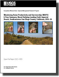
The MAPS banding station was located on NOLF, which encompasses about 509 hectares (ha) in southwestern San Diego County, including 112 ha of roads and developed areas. The site is 16 kilometers (km) south of Naval Air Station North Island (NASNI) and 2.4 km north of the United States-Mexico border. Navy lands extend into the Tijuana River National Estuarine Research Reserve, co-managed by USFWS, the National Oceanic and Atmospheric Administration, and California State Parks (fig. 1). Parts of NOLF are managed cooperatively with the Tijuana Slough National Wildlife Refuge under a memorandum of understanding between NASNI and the USFWS relating to the protection of natural resources. Vegetation at the station was a mix of riparian willow (Salix spp.) forest dominated by arroyo willow (S. lasiolepis), red willow (S. laevigata), black willow (S. gooddingii), and mule fat (Baccharis salicifolia); and riparian scrub dominated by mule fat and sandbar willow (S. exigua).
Location of the Monitoring Avian Productivity and Survivorship banding station, Naval Outlying Landing Field, Imperial Beach, California.
Bird Banding
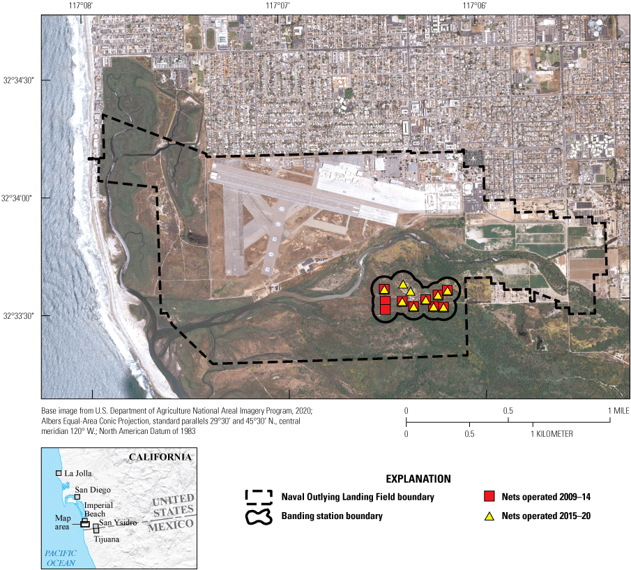
Bird banding at NOLF followed the standardized MAPS protocol (DeSante and others, 2021). Ten mist nets, placed a minimum of 65 meters (m) apart, were erected in fixed locations selected for their potential to capture birds moving through vegetation (table 1; fig. 2). In 2015, two nets were discontinued when trails were closed to discourage unlawful access and were replaced by two new net lanes within the station. Mist nets were made of 30-millimeter (mm) mesh black nylon and were 12-m long by 2.6-m high with four trammels (pockets) running the length of the net. Nets were suspended from vertical aluminum poles anchored by permanent rebar stakes and covered a vertical area ranging from about 0.25 to 2.50 m above ground. Nets were opened within 30 minutes of dawn and remained open for 6 hours, typically until between 1200 and 1300 Pacific Daylight Time (PDT). Nets were not operated during inclement weather such as strong wind, rain, extreme heat, or cold. If nets were not operated for a minimum of 3 hours during a particular period (for instance, if nets were closed early because of inclement weather), we scheduled a make-up day during the same period. On the make-up day, we opened the nets at the approximate time that nets were closed on the short day and then closed the nets when the 6 hours intended for the period were reached.
Table 1.
Global Positioning System locations of mist nets at Monitoring Avian Productivity and Survivorship banding station, Naval Outlying Landing Field, Imperial Beach, California.[Coordinates are in World Geodetic System of 1984 (WGS 84). Nets 5 and 6 were operated 2009–14; nets 11 and 12 were operated 2015, 2017–20. All other nets were operated 2009–15 and 2017–20. For net numbers, see figure 2]
Net locations at Monitoring Avian Productivity and Survivorship banding station, Naval Outlying Landing Field, Imperial Beach, California.
Nets were checked every 30–40 minutes by operators working circuits. Hummingbirds, game birds, and other non-passerines were not banded but were identified by species, age, and sex (when possible) and then released. Birds were removed from nets, held in cloth bags labeled with the net number, and taken to a central processing location where they were banded with numbered Federal aluminum bands. From 2014 to 2019, Least Bell’s Vireo (Vireo bellii pusillus) captured at this MAPS banding station were color-banded with a unique color combination for visual identification as part of a separate survey effort for this species (10[A][1][a] federal recovery permit number ESPER0004080). Using the Identification Guide to North American Birds (Pyle, 1997) as a reference, data recorded for each individual captured (all species) included age, sex, skull ossification, breeding condition, weight, wing chord, fat deposition, feather wear, and molt status. Birds that already had bands when captured also were processed, and their band numbers were recorded. These birds were considered recaptures. We recorded only the initial capture of a bird on each banding day (we did not record same-day recaptures). A bird was considered a recapture on each unique day it was captured after its original banding. Birds were held for 5–45 minutes depending on the number of birds captured during one net run. After processing, juveniles, brooding females, and resident birds from the more distant nets were released near the net in which they had been captured, whereas all other birds were released at the central processing location. A list of all birds observed was kept for each banding day, including species not captured and their possible breeding status at the MAPS banding station. A minimum of four personnel typically operated the MAPS banding station.
Banding Schedule
The MAPS banding station was operated 1 day during every 10-day period from April 1 to August 8 (for a total of 13 banding days per year), except in 2020, when flooding prevented our access to the banding station for the first period in April. Most North American MAPS stations operate during the standard MAPS season (May 1–August 8). Starting in 2012, we added netting periods in April to accommodate earlier breeding species, such as Orange-crowned Warbler (Leiothlypis celata), and for comparisons with other MAPS banding stations in San Diego County, which begin operation in April (Lynn and others, 2018; B. Kus, U.S. Geological Survey, unpub. data, 2021).
Data Analysis
Captures
All banding data were entered into MAPSPROG (the IBP data entry program) for verification and error-checking, which also included cross-checking against data from previous years. Finalized MAPSPROG data were submitted to IBP and Naval Base Coronado each year. This report presents a summary of banding data from 2014 to 2020 and analyses of longer-term population trends, productivity, and survivorship from 2009 to 2020 (2009–13 data are available in Lynn and others, 2015).
Bird captures were quantified by species, age, sex, and number of captures for each year. The total number of captures (including newly banded birds, captured but unbanded birds, and all recaptures) was used to create a captured species list and a total count of captures per species for the MAPS banding station. For analyses, year-unique captures were the total number of individuals captured for the first time each year, including newly banded birds, first-time recaptures of birds originally banded in previous years, and unbanded birds. The population size for each species was the number of year-unique adult captures, corrected for effort (see the “Effort Corrections” section). Hummingbirds and other unbanded birds were included in the total count of captures, the captured species list, and year-unique captures, but they were not included in further analyses of productivity or survival because we could not determine individual identity. We included hummingbirds and other unbanded captures as separate individuals in year-unique captures even though some may have been captured more than once during the season. We calculated species richness defined as the number of species captured at the MAPS banding station, relative species abundance defined as the proportion of all year-unique captures, corrected for effort (see the “Captures” and “Effort Corrections” sections) represented by a particular species, and sex and age ratios (to determine the structure of the population) for all species captured.
Effort Corrections
Netting effort varied between years as a result of adding netting periods in April (starting in 2012) and missing periods or truncating days in response to inclement weather or other logistical constraints. Because of this variation, the intended effort (10 nets run for 6 hours per period or 60 intended net-hours per period) in a survey was not always met. The timing of missed or gained effort during a season or period can alter capture rate estimates and thus skew vital rate calculations. For example, the ratio of juveniles to adults resulting from not capturing adults during times when nets were closed before young-of-the-year fledge or not capturing juveniles during times when nets were closed after fledging, could result in over- or under-estimating productivity, respectively.
We followed methods developed by DeSante and others (2015) to summarize effort and capture data for a single station and to correct capture data for inconsistencies in seasonal effort with modifications for time of capture during the day. Effort corrections began by dividing the banding day into five time bins relative to sunrise: (1) 1 hour before sunrise to 1 hour after sunrise; (2) 1‒2 hours after sunrise; (3) 2‒3 hours after sunrise; (4) 3‒4 hours after sunrise; and (5) more than 4 hours after sunrise. We then compiled the actual effort expended (number of hours nets were open multiplied by number of nets that were open) for each time bin, each sampling period, and each year (Ab,p,t, where b is time bin [1‒5], p is sampling period [1‒13], and t is year [2009‒20, excluding 2016 when the station was not operated]). Second, we summed actual effort for all time bins within a period to get the total actual effort per period:
wheree
is total actual effort,
p
is sampling period (1–13),
t
is year 2009–20 (excluding 2016 when the station was not operated),
b
is time bin (1–5), and
A
is actual effort for each time bin.
H
is the proportion of actual effort per period represented by each time bin,
b
is time bin (1–5),
p
is sampling period (1–13),
t
is year 2009–20 (excluding 2016 when the station was not operated),
A
is actual effort for each time bin, and
e
is total actual effort.
h
is the proportional difference between intended and actual effort,
b
is time bin (1–5),
p
is sampling period (1–13),
t
is year 2009–20 (excluding 2016 when the station was not operated),
I
is intended effort per time bin, and
A
is actual effort per time bin.
Captures per year were calculated by age and by species for all year-unique captures (including birds of undetermined age). To calculate captures per year using effort correction, we began by summing the number of year-unique captures for each species by time bin (nAb,p,t for adults, nJb,p,t for juveniles, and nTb,p,t for all captures). Next, we summed the total number of year-unique captures for each species by period by year:
whereNA
is total number of year-unique adults captured per period per year,
p
is sampling period (1–13),
t
is year 2009–20 (excluding 2016 when the station was not operated),
b
is time bin (1–5), and
nAb,p,t
is the number of year-unique adults captured for each time bin.
is total number of year-unique juveniles captured per period per year,
p
is sampling period (1–13),
t
is year 2009–20 (excluding 2016 when the station was not operated),
b
is time bin (1–5), and
is the number of year-unique juveniles captured for each time bin.
NT
is total number of year-unique captures of all ages per period per year,
p
is sampling period (1–13),
t
is year 2009–20 (excluding 2016 when the station was not operated),
b
is time bin (1–5), and
nTb,p,t
is the number of year-unique captures of all ages for each time bin.
δA
is the proportion of adult captures in a period represented by each time bin,
b
is time bin (1–5),
p
is sampling period (1–13),
t
is year 2009–20 (excluding 2016 when the station was not operated),
nAb,p,t
is the number of year-unique adults captured for each time bin, and
NA
is the total number of year-unique adults captured per period per year.
is for the proportion of juveniles captured in a period represented by each time bin,
b
is time bin (1–5),
p
is sampling period (1–13),
t
is year 2009–20 (excluding 2016 when the station was not operated),
is the number of year-unique juveniles captured for each time bin, and
is total number of year-unique juveniles captured per period per year.
is for proportion of all ages captured in a period represented by each time bin,
b
is time bin (1–5),
p
is sampling period (1–13),
t
is year 2009–20 (excluding 2016 when the station was not operated),
is the number of year-unique captures of all ages for each time bin, and
is total number of year-unique captures of all ages per period per year.
is the effort correction factor for adults,
b
is time bin (1–5),
p
is sampling period (1–13),
t
is year 2009–20 (excluding 2016 when the station was not operated),
is the proportion of adult captures in a period represented by each time bin,
h
is the proportional difference between intended and actual effort, and
H
is the proportion of actual effort per period represented by each time bin.
is the effort correction factor for juveniles,
b
is time bin (1–5),
p
is sampling period (1–13),
t
is year 2009–20 (excluding 2016 when the station was not operated),
is the proportion of juvenile captures in a period represented by each time bin,
is the proportional difference between intended and actual effort, and
is the proportion of actual effort per period represented by each time bin.
is the effort correction factor for all captures,
b
is time bin (1–5),
p
is sampling period (1–13),
t
is year 2009–20 (excluding 2016 when the station was not operated),
is the proportion of all captures in a period represented by each time bin,
is the proportional difference between intended and actual effort, and
is the proportion of actual effort per period represented by each time bin.
is the corrected number of adults,
t
is year 2009–20 (excluding 2016 when the station was not operated),
p
is sampling period (1–13),
b
is time bin (1–5),
is the total number of year-unique adults captured per period per year, and
is the effort correction factor for all adult captures.
is the corrected number of juveniles,
t
is year 2009–20 (excluding 2016 when the station was not operated),
p
is sampling period (1–13),
b
is time bin (1–5),
is the total number of year-unique juveniles captured per period per year, and
is the effort correction factor for all juvenile captures.
is the corrected number of all captures,
t
is year 2009–20 (excluding 2016 when the station was not operated),
p
is sampling period (1–13),
b
is time bin (1–5),
is the total number of year-unique captured of all ages per period per year, and
is the effort correction factor for all captures.
In table 2, we present an example of effort correction for a hypothetical period 5 banding day in 2016. For this example, 10 nets were open for 5 hours each, and all nets were closed 1 hour early because of excessive wind. Total actual effort (e5,2016) was 50 hours, and total year-unique captures in period 5 (NT5,2016) was 100. For this example, the actual effort in time bin 5 (that is, more than 4 hours after sunrise) was 10 hours, while the intended effort was 20 hours. This corrected the number of captures (nT5,5,2016) upward for that time bin, from 10 captures to 12.5 captures. Therefore, the total number of effort-corrected captures for period 5 in 2016 (CT2016) was 103 (rounded from 102.5).
Table 2.
Example of effort correction for a hypothetical banding period when actual netting hours were less than intended netting hours.Focal Species
For a subset of resident and migratory focal species that breed at the station, we examined seasonal and annual variation in capture rates, productivity (the ratio of juveniles to adults captured, as described later in the “Annual Productivity” section), adult survival (based on analysis of recapture rates using Program MARK, as described later in the “Annual Survival” section), and population trends. All species captured at the MAPS station, except Black-throated Magpie-jay (Calocitta colliei), were considered migratory species covered under the Migratory Bird Treaty Act (U.S. Fish and Wildlife Service, 2020; appendix 1, tables 1.1, 1.2); however, some species considered migratory birds under the Act are known to be year-round residents in southwestern San Diego County, and therefore, were considered resident species in our analyses. According to the MAPS protocol, species were considered breeders if they exhibited persistent territorial singing during the height of the breeding season, or hard evidence of breeding (observation of nest, fledglings, etc.) at the station (as opposed to within the larger surrounding area) at least once during station operation. Year-round resident species in analyses of population trends, productivity, survival, and predictors of population change included Bushtit (Psaltriparus minimus), Wrentit (Chamaea fasciata), House Wren (Troglodytes aedon), Song Sparrow (Melospiza melodia), Common Yellowthroat (Geothlypis trichas), and Orange-crowned Warbler. We considered Orange-crowned Warbler to be resident because the species was present at the MAPS station year-round although it was possible that different subspecies occupied the area in the winter than during the breeding season. Nevertheless, Orange-crowned Warbler populations likely did not move long distances between seasons and therefore were subject to climatic conditions similar to the MAPS station during the non-breeding season. One migratory species, Least Bell’s Vireo, known to winter outside southwestern San Diego County, also was included as a focal species in analyses of population trends, productivity, survival, and predictors of population change.
Seasonal and Annual Variation in Captures
Seasonal and annual variations in capture rates for adults and juveniles were examined for locally breeding focal species that constituted 5 percent or more of captures in at least 6 years over the entire span of the MAPS station operation (2009–20). Bushtit and Orange-crowned Warbler constituted more than 5 percent of captures in all 11 years. Song Sparrow constituted more than 5 percent of captures in 10 of the 11 years, and Common Yellowthroat constituted more than 5 percent of captures in 9 of the 11 years. Wilson’s Warbler (Cardellina pusilla) constituted 5 percent or more of captures in 7 of the 11 years, but only wintered at or migrated through the MAPS banding station; therefore, we did not include it as a focal species. We included a fifth species, Least Bell’s Vireo (a migratory species that breeds at the station and winters south of the station), which constituted 1–5 percent of captures each year, to examine the status of this Federal- and State-protected species at NOLF. We examined the seasonal variation in captures for each of these species by plotting captures by MAPS period. We calculated mean captures from 2014 to 2020 by MAPS period for species that could be assigned an age (adults versus juveniles) and compared these to the annual capture rates of adults and juveniles to examine age-related seasonal trends.
We also examined age structure in captures over the entire span of the MAPS station operation by plotting annual captures of each focal species by age from 2012 to 2019, excluding years when early banding periods were missed (2009, 2010, 2011, and 2020). We examined annual population trends in adult captures from 2012 to 2019 for each of the five focal species using Pearson’s correlations. Any P-values less than 0.10 indicated that populations of that species significantly increased or decreased from 2012 to 2019.
Annual Productivity, Survival, and Predictors of Population Size
Seven focal species, the five focal species analyzed for population trends plus two additional resident species (Wrentit and House Wren), were selected for calculations of annual productivity and survival from 2009 to 2020, based on criteria presented by IBP for survival analyses. These criteria include (1) at least 2.5 individuals of the species captured per year, with a minimum of 30 year-unique captures; (2) at least 2 recaptures; and (3) survival and recapture probability not equal to 0 or 1.
Climate Variables
A number of climate variables had the potential to influence productivity and survival of the seven species we selected for these analyses. We selected climate variables based on their potential to explain annual life stages of the focal species. Specifically, we selected bio-year precipitation, or total precipitation from July 1 (year x−1) to June 30 (year x), a date range which encompasses the entire winter, the typical period of high rainfall in southern California. We also divided annual precipitation into two periods, early winter precipitation (October 1[year x−1]–December 31[year x−1]) and late winter precipitation (January 1[year x]–March 31[year x]), which likely influences the timing of increased availability of food resources (seeds, fruits, and insects). We also selected mean maximum daily temperature in August[year x−1] and mean minimum daily temperature in December[year x−1] to represent the hottest and coldest periods of the year. Mean breeding season temperature (mean temperature from March 1[year x] to June 30[year x]) had the potential to influence breeding productivity. Mean bio-year temperature (mean temperature from July 1 [year x−1] to June 30 [year x]) provided an annual measure of potential climate change within the same period as bio-year precipitation, and it can be useful in comparing with results from other regions. Daily temperature and precipitation data were gathered from the Brown Field Municipal Airport (National Oceanic and Atmospheric Administration, 2022), 11 km east of the MAPS station, for the years that the MAPS station was operated. Daily temperature and precipitation data also were gathered from Brown Field Municipal Airport for the years prior to station operation, when available, including 1945–46, 1954–61, and 1997–2008, to compare historical trends to trends during station operation. We used two-sample Student’s t-tests and Wilcoxon signed-rank tests to compare the means of precipitation and temperature before and during station operation. Any P-values less than 0.10 indicated that precipitation and temperature were significantly different before station operation than they were during station operation.
Annual Productivity
We used generalized linear models with a gaussian probability structure to model the effects of climate variables on annual productivity. Annual productivity is defined as the ratio of effort-corrected young (juvenile) captures to effort-corrected adult captures (CJt/CAt). For each of the seven focal-plus species, we created models relating annual productivity (the response variable) to mean breeding season temperature, mean bio-year temperature, bio-year precipitation, early winter precipitation, and late winter precipitation (predictor variables). To simplify interpretation of model results, we standardized the predictor variables before analysis by subtracting the mean and dividing by the standard deviation. We excluded 2018 Wrentit productivity from our analyses because unique-year captures were unusually low (5 individuals), and 80 percent (4/5) were juveniles, creating an artificially high productivity estimate for that year.
We created a set of a priori models containing the predictor variables and used an information-theoretic approach (Akaike’s Information Criterion for small sample sizes, or AICc) to evaluate support for each model (Burnham and Anderson, 2002). To build our model set, we first generated a constant (null) model to serve as a reference and a set of simple models, each of which contained a single predictor variable. Next, we began creating more complex models by adding other predictor variables to each of the simple models and evaluating them relative to the simpler model, eliminating those that did not improve on the simpler model by at least 2 AICc. All remaining models were ranked such that the highest-ranked model had the lowest AICc. Models were considered well supported if the ΔAICc (difference in AICc from the highest-ranked model) was less than 2. Only models with an AICc weight of at least 0.05 were presented in the final model set. After finalizing our model set, we evaluated the contribution of predictor variables to each model by examining the 90-percent confidence interval associated with the beta estimate for each variable. If the 90-percent confidence interval did not include 0, we had 90-percent confidence that the beta estimate differed from 0, and therefore, we determined that the variable likely contributed to the model. Models were created and summarized using the MuMIn package (version 1.43.17; Bartoń, 2020) in R (R Core Team, 2022).
Annual Survival
We analyzed annual survival of adults for the seven focal-plus species in Program MARK (White and Burnham, 1999) using the RMark package (Laake, 2013) in R (R Core Team, 2022). Survival analysis in Program MARK accounts for individuals that were present but not captured by modeling both survivorship and recapture probability. We estimated adult survival but not first-year survival because first-year survival was low for all species, and therefore, we could not differentiate the probability of survival from recapture probability. Birds that originally were banded as juveniles (during their hatching year) were included in analyses as adults in subsequent years. We created encounter histories for each year from 2009 to 2020, coding capture or recapture as 1 and no capture as 0.
Effort was not constant across years because no nets were opened in early banding periods in some years (2009, 2010, 2011, and 2020). To determine whether differences in effort had an effect on survival analyses, we modeled recapture probability in two ways for each species: (1) one model with constant recapture probability and (2) one model with time-varying recapture probability (allowing recapture probability to vary by year), using constant survival in both models. We compared the AICc of the two models and selected the model with the lowest AICc. Models with constant recapture probability ranked well above models with time-varying recapture probability for all species except Orange-crowned Warbler. Therefore, for all species except Orange-crowned Warbler, we used constant recapture probability in all models. For Orange-crowned Warbler, we allowed recapture probability to vary by year in all models. Because the MAPS station was not operated in 2016, annual survival for 2015–16 and 2016–17 was estimated by MARK by interpolating from other years.
Survival models were created to examine the effects of sex and climate variables on annual survival of adults. Climate variables included bio-year precipitation, early winter precipitation, late winter precipitation, mean bio-year temperature, mean maximum daily temperature in August, and mean minimum daily temperature in December. For species that remained at the MAPS station during the winter (Bushtit, Orange-crowned Warbler, Song Sparrow, Common Yellowthroat, Wrentit, and House Wren), survival models were created with precipitation and temperature during the bio-year ending in the current MAPS season. For species that migrated away from the MAPS station during the winter (Least Bell’s Vireo), survival models were created with precipitation during the bio-year ending in the previous MAPS season because migrants were absent from the MAPS banding station from September to March of the current bio-year and, thus, their survival likely was more influenced by precipitation at the MAPS banding station during the previous bio-year than the current bio-year. Similarly, we did not include mean minimum daily temperature in December in models for Least Bell’s Vireo because the species was not present at the MAPS banding station during December. Model sets were created and evaluated using information theoretic approach (AICc; see the “Annual Productivity” section).
Predictors of Population Change
Breeding productivity and annual survival are inherently linked to changes in bird populations. Absent other influences, higher breeding productivity and higher annual survival should result in increased population size. We used multiple regression to evaluate the contribution of breeding productivity and annual survival to population change (λ, or N[year x+1]/N[year x]) for each of the seven focal-plus species. First, we estimated λ using Pradel reverse-time capture-mark-recapture models (Pradel, 1996) in Program MARK. For all Pradel models, we used constant survival and recapture probabilities to isolate annual λ. Then, we used annual productivity in yearx−1 and annual survival estimates from yearx−1 to yearx as predictors, and λ from yearx−1 to yearx as the response variable in multiple regression analysis. For each predictor within a multiple regression model, P-values less than 0.10 indicate that the predictor, in isolation, significantly influenced the population change of that species. An overall P-value less than 0.10 for the overall multiple regression model indicates that population change was influenced by the combination of predictors.
Data were analyzed using Program R. Analyses were considered significant if P≤0.10. Means are presented with standard deviations. All data from NOLF 2009 to 2013 used in analyses can be found in Lynn and others (2015).
Results
Overview of Captures
In 4,603 net-hours (751±51 net-hours per year) during the 2014–20 MAPS seasons, we had a total of 3,543 captures (591±176 captures per year; table 3). Of the 3,543 total captures, 2,702 were newly banded, 258 were individuals recaptured from previous years, and 304 were released unbanded (218 hummingbirds and 86 other birds that escaped before banding or were intentionally released unbanded, such as game birds) for a total of 3,264 year-unique captures (544±155 unique captures per year). We captured 68 species, 39 of which were confirmed or likely breeders at the MAPS banding station (table 3; appendix 1, table 1.1; unidentified species were not included in the species total).
Table 3.
Total number of birds captured, banded, recaptured, and released unbanded at Naval Outlying Landing Field, Imperial Beach, California, 2014–20.[Species: See appendix 1 (tables 1.1, 1.2) for common and scientific names. Total captures: Includes multiple captures of some individuals]
Of note, in 2014, we recaptured a Rufous Hummingbird (Selasphorus rufus) that originally had been banded in Tallahassee, Florida, in January 2014. This hummingbird travelled 3,100 km between its original banding station and our nets.
Sensitive Species
Nineteen sensitive species were detected at NOLF (12 captured and 7 observed only; appendix 1, tables 1.1, 1.2). We captured one State and Federally endangered species, Least Bell’s Vireo, one Federally threatened species, Coastal California Gnatcatcher (Polioptila californica californica), one State endangered species, Willow Flycatcher (Empidonax traillii), and two State species of concern, Yellow-breasted Chat (Icteria virens), and Yellow Warbler (Setophaga petechia; appendix 1, table 1.1; Shuford and Gardali, 2008; U.S. Fish and Wildlife Service, 2020; California Department of Fish and Wildlife, 2023). One additional State species of concern, Northern Harrier (Circus hudsonius), was observed at the MAPS banding station but was not captured (appendix 1, table 1.2; Shuford and Gardali, 2008). Peregrine Falcon (Falco peregrinus) and White-tailed Kite (Elanus leucurus), California State fully protected species, also were observed at the MAPS banding station (California Department of Fish and Wildlife, 2021). Seven Federal bird species of conservation concern—Calliope Hummingbird (Selasphorus calliope), Rufous Hummingbird, Allen’s Hummingbird (Selasphorus sasin), Nuttall’s Woodpecker (Dryobates nuttallii), Wrentit, California Thrasher (Toxostoma redivivum), and Lawrence’s Goldfinch (Spinus lawrencei)—were captured. Four additional Federal bird species of conservation concern—Willet (Tringa semipalmata), Western Gull (Larus occidentalis), California Gull (Larus californicus), and Bullock’s Oriole (Icterus bullockii)—were observed but not captured (appendix 1, tables 1.1, 1.2). Eleven of the sensitive species breed at NOLF (nine captured and two observed only).
Sixty-five Least Bell’s Vireo were captured and banded from 2014 to 2020. Four additional Least Bell’s Vireos captured prior to 2014 were recaptured between 2014 and 2020, for a total of 69 individual Least Bell’s Vireos captured from 2014 to 2020. Nine of the 69 vireos were recaptured in subsequent years (12 total recaptures between 2014 and 2020). Of the 69 individually banded vireos, 49 were given unique color band combinations, and 20 were banded with a single numbered metal band.
Capture Rates
The overall effort-corrected capture rate was 43±30 captures per MAPS period for all years combined (range 7–163 captures; table 4). Effort-corrected capture rates by year ranged from 240 to 745 captures with 2014 and 2018 being the highest capture years. Period 2 in 2014 had the highest effort-corrected capture rate of 163, a result of capturing a large number of birds (128 individuals) during a truncated survey day (0555–0910 PDT) when nets were closed early because of rain.
Table 4.
Capture rate of year-unique individuals by Monitoring Avian Productivity and Survivorship (MAPS) period and year at Naval Outlying Landing Field, Imperial Beach, California, 2014–20.[Year-unique captures were the total number of new captures, first-time recaptures, and unbanded birds captured in that year. Effort-corrected captures were year-unique captures corrected for effort following methods in DeSante and others (2015). Abbreviation: —, no data]
Species Richness
The number of species captured ranged from 37 to 46 per year (tables 5–10). Daily species richness among captures averaged highest in early May, although in 3 years (2015, 2017, and 2020), species richness peaked in early to mid-April. Overall, species richness averaged 43±4 per year.
Table 5.
Number of captures by Monitoring Avian Productivity and Survivorship (MAPS) period and date at Naval Outlying Landing Field, Imperial Beach, California, 2014.[Captures were corrected for effort following methods in DeSante and others (2015). Species: See appendix 1 (tables 1.1, 1.2) for common and scientific names. Effort-corrected totals were rounded to integers; annual effort corrected total captures were calculated from actual (non-integer) values. Abbreviations: mm-dd-yy, month-day-year; —, no data]
Table 6.
Number of captures by Monitoring Avian Productivity and Survivorship (MAPS) period and date at Naval Outlying Landing Field, Imperial Beach, California, 2015.[Captures were corrected for effort following methods in DeSante and others (2015). Species: See appendix 1 (tables 1.1, 1.2) for common and scientific names. Effort-corrected totals were rounded to integers; annual effort corrected total captures were calculated from actual (non-integer) values. Abbreviations: mm-dd-yy, month-day-year; —, no data]
Table 7.
Number of captures by Monitoring Avian Productivity and Survivorship (MAPS) period and date at Naval Outlying Landing Field, Imperial Beach, California, 2017.[Captures were corrected for effort following methods in DeSante and others (2015). Species: See appendix 1 (tables 1.1, 1.2) for common and scientific names. Zero effort-corrected captures resulted from nets that remained open beyond the prescribed 6 hours. Abbreviations: mm-dd-yy, month-day-year; —, no data]
Table 8.
Number of captures by Monitoring Avian Productivity and Survivorship (MAPS) period and date at Naval Outlying Landing Field, Imperial Beach, California, 2018.[Captures were corrected for effort following methods in DeSante and others (2015). Species: See appendix 1 (tables 1.1, 1.2) for common and scientific names. Effort-corrected totals were rounded to integers; annual effort corrected total captures were calculated from actual (non-integer) values. Abbreviations: mm-dd-yy, month-day-year; —, no data]
Table 9.
Number of captures by Monitoring Avian Productivity and Survivorship (MAPS) period and date at Naval Outlying Landing Field, Imperial Beach, California, 2019.[Captures were corrected for effort following methods in DeSante and others (2015). Species: See appendix 1 (tables 1.1, 1.2) for common and scientific names. Abbreviations: mm-dd-yy, month-day-year; &, and; —, no data]
Table 10.
Number of captures by Monitoring Avian Productivity and Survivorship (MAPS) period and date at Naval Outlying Landing Field, Imperial Beach, California, 2020.[Captures were corrected for effort following methods in DeSante and others (2015). Species: See appendix 1 (tables 1.1, 1.2) for common and scientific names. Abbreviations: mm-dd-yy, month-day-year; —, no data]
Relative Species Abundance
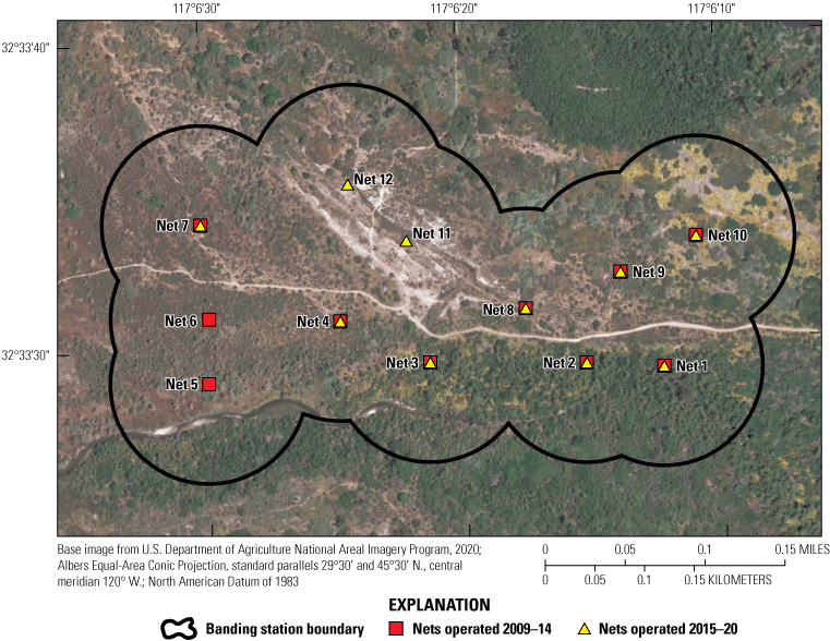
Bushtit was the most abundant species, with 372 effort-corrected captures and a mean of 62±22 effort-corrected captures per year (figs. 3A–E; tables 5–10). Orange-crowned Warbler was the second most abundant species, with 315 effort-corrected captures and a mean of 53±22 effort-corrected captures per year. The third most abundant species was Wilson’s Warbler, with 296 effort-corrected captures (49±35 effort-corrected captures per year). House Finch (Haemorhous mexicanus) was the fourth most abundant species, with 288 effort-corrected captures (48±34 effort-corrected captures per year), followed by Song Sparrow, with 230 effort-corrected captures (38±16 effort-corrected captures per year), and Common Yellowthroat, with 177 effort-corrected captures (30±21 effort-corrected captures per year). These six species each accounted for at least 5 percent of all effort-corrected captures per year and together accounted for 51 percent of all effort-corrected captures during 2014–20. Five of these species, Bushtit, Orange-crowned Warbler, Wilson’s Warbler, Song Sparrow, and House Finch, accounted for at least 5 percent of effort-corrected annual captures during at least 4 years from 2014 to 2020. Additional species that accounted for 5 percent or more of the effort-corrected captures in at least 1 year included Common Yellowthroat, Warbling Vireo (Vireo gilvus), Pacific-slope Flycatcher (Empidonax difficilis), Anna’s Hummingbird (Calypte anna), House Wren, Audubon’s Warbler (Setophaga coronata auduboni), Swainson’s Thrush (Catharus ustulatus), Least Bell’s Vireo, Yellow Warbler, and White-crowned Sparrow (Zonotrichia leucophrys).
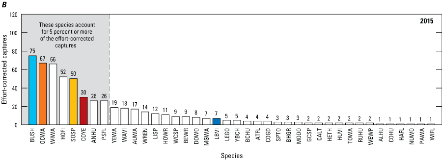
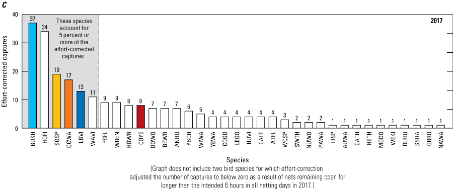
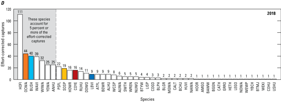
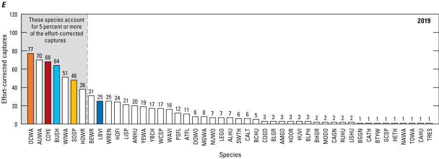
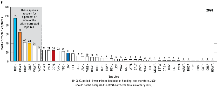
Number of year-unique and effort-corrected captures per species for the years A, 2014; B, 2015; C, 2017; D, 2018; E, 2019; and F, 2020, Naval Outlying Landing Field, Imperial Beach, California, 2014–20. Species that accounted for 5 percent or more of the effort-corrected captures in at least 6 years between 2009 and 2020 were given colored bars to track annual variation. Bushtit was the only species that constituted more than 5 percent of the captures every year. See appendix 1 for common and scientific names. Capture rates were corrected for effort following methods in DeSante and others (2015).
Seasonal and annual captures varied for each of the five focal bird species (figs. 4A–E). Captures of Least Bell’s Vireos were few throughout the MAPS season every year, with a peak in captures in late June corresponding to an increase in juvenile captures in 2015, 2017, 2019, and 2020 (fig. 4A). Bushtit had two identifiable peaks in seasonal captures, one in May and one in late June to early July (fig. 4B). The Bushtit peak in mid to late May corresponded to an increase in adult captures and occurred in all years except 2017. The peak in Bushtit captures in late June to early July corresponded to an increase in juvenile captures and occurred in all years. In general, Song Sparrow captures were highest in April and lowest in June and July, although there was some seasonal variation in captures between years (fig. 4C). Song Sparrow adult captures were highest in April and decreased throughout the MAPS season. Juvenile captures began in mid-April and remained relatively constant throughout the remainder of the MAPS season. Orange-crowned Warbler captures were highest in early to mid-April in most years, prior to the start of the standard MAPS season (May 1; fig. 4D), corresponding to the peak in mean adult captures. A secondary peak in Orange-crowned Warbler captures occurred in May, when mean juvenile captures increased. For Common Yellowthroat, captures varied between years and MAPS periods, although there was a peak in captures in mid-April in 2014, 2019, and 2020 that was exclusively comprised of adults (fig. 4E). Similar to Song Sparrows, mean adult captures of Common Yellowthroats decreased throughout the MAPS banding season. No juvenile Common Yellowthroats were captured in any year until early May, and thereafter, the mean juvenile capture rate generally increased through the end of the MAPS banding season.
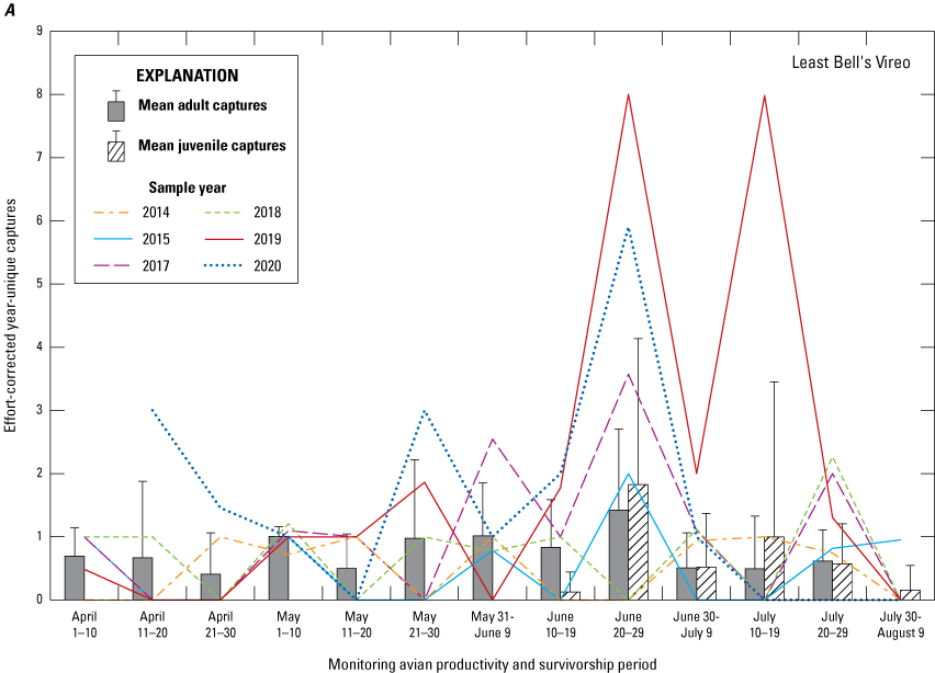
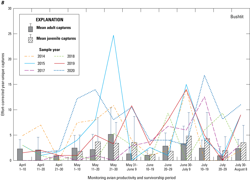
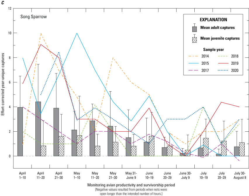
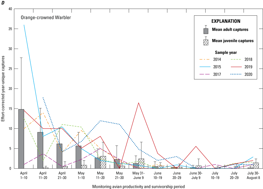
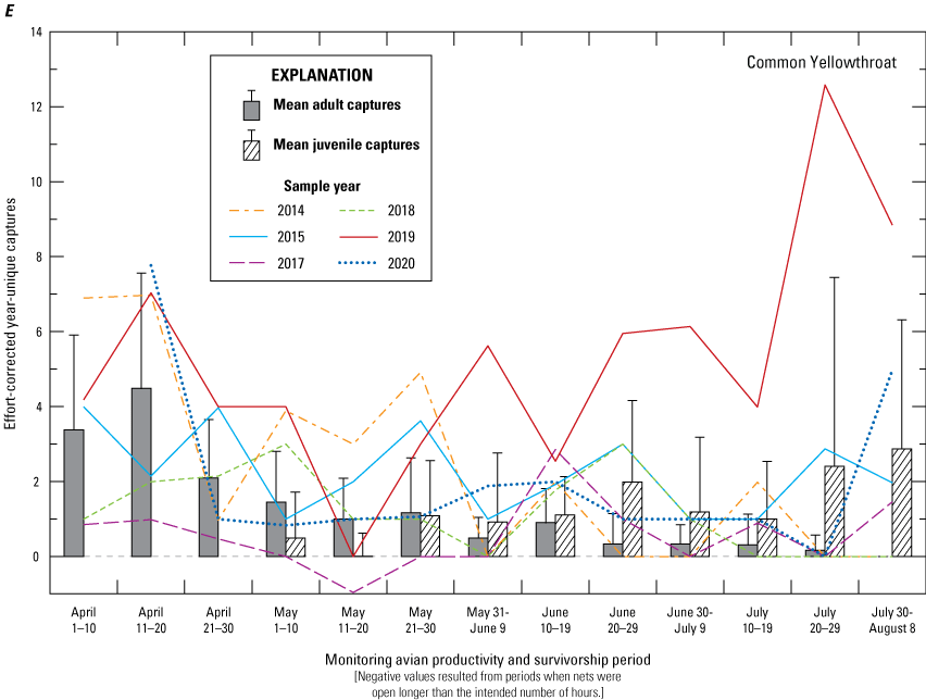
Seasonal and annual variation in the effort-corrected number of year-unique captures of the bird species A, Least Bell’s Vireo; B, Bushtit; C, Song Sparrow; D, Orange-crowned Warbler; and E, Common Yellowthroat at Naval Outlying Landing Field, Imperial Beach, California, 2014–20. Means for adults and juveniles are across years within each banding period. See appendix 1 for common and scientific names. Capture rates were corrected for effort following methods in DeSante and others (2015).
Sex and Age Structure
The overall sex ratio of known-sex adult captures was slightly skewed towards males for all species combined from 2014 to 2020 (54:46 male:female for 2014–20). The male:female ratios ranged from 44:56 in 2014 to 60:40 in 2019 (tables 11–16). Adults averaged 73±12 percent of known-age captures per year (range 59–94 percent), and juveniles averaged 27±12 percent (range 6–41 percent).
Table 11.
Sex and age of year-unique bird captures at Naval Outlying Landing Field, Imperial Beach, California, 2014.[Species: See appendix 1 (tables 1.1, 1.2) for common and scientific names. Age: HY, hatching year; AHY, after hatching year; SY, second year; ASY, after second year; ATY, after third year; I, indeterminant]
Table 12.
Sex and age of year-unique bird captures at Naval Outlying Landing Field, Imperial Beach, California, 2015.[Species: See appendix 1 (tables 1.1, 1.2) for common and scientific names. Age: HY, hatching year; AHY, after hatching year; SY, second year; ASY, after second year; ATY, after third year; I, indeterminant]
Table 13.
Sex and age of year-unique bird captures at Naval Outlying Landing Field, Imperial Beach, California, 2017.[Species: See appendix 1 (tables 1.1, 1.2) for common and scientific names. Age: HY, hatching year; AHY, after hatching year; ASY, after second year; ATY, after third year; I, indeterminant]
Table 14.
Sex and age of year-unique bird captures at Naval Outlying Landing Field, Imperial Beach, California, 2018.[Species: See appendix 1 (tables 1.1, 1.2) for common and scientific names. Age: HY, hatching year; AHY, after hatching year; SY, second year; ASY, after second year; ATY, after third year; I, indeterminant; TY, third year]
Table 15.
Sex and age of year-unique bird captures at Naval Outlying Landing Field, Imperial Beach, California, 2019.[Species: See appendix 1 (tables 1.1, 1.2) for common and scientific names. Age: HY, hatching year; AHY, after hatching year; SY, second year; ASY, after second year; TY, third year; ATY, after third year; I, indeterminant]
Table 16.
Sex and age of year-unique bird captures at Naval Outlying Landing Field, Imperial Beach, California, 2020.[Species: See appendix 1 (tables 1.1, 1.2) for common and scientific names. Age: HY, hatching year; AHY, after hatching year; SY, second year; ASY, after second year; TY, third year; ATY, after third year; I, indeterminant]
A mean of 389±140 adults (effort-corrected) were captured per year. During 4 of 6 years, the adult capture rate was similar to the 6-year mean (within 1 standard deviation). However, in 2014, the adult capture rate was 52 percent greater than the 6-year mean (593 effort-corrected captures, driven primarily by one period when a large number of birds were captured during a truncated netting day). In 2017, the adult capture rate was 60 percent less than the 6-year mean (157 effort-corrected captures).
A mean of 153±96 juveniles (effort-corrected) were captured per year. Like adults, the juvenile capture rate was within 1 standard deviation of the 6-year mean during 4 of the 6 years. In 2017, the juvenile capture rate was 65 percent lower than the 6-year mean (54 effort-corrected captures) and in 2019, the juvenile capture rate was 101 percent greater than the 6-year mean (308 effort-corrected captures). Juveniles of 26 species were captured between 2014 and 2020 (17±5 species per year). The six species with the most juveniles captured (Bushtit, House Finch, Anna’s Hummingbird, Song Sparrow, Common Yellowthroat, and Orange-crowned Warbler, in descending order of abundance) comprised 72 percent of the total number of juvenile captures between 2014 and 2020. The species that contributed the most to juvenile captures each year were House Finch in 2014, 2017, and 2018, Bushtit in 2015 and 2020, and Common Yellowthroat in 2019.
Population Trends
Between 2012 and 2019 (years with no missed banding periods), the age structure of captures varied by year and by species for the five breeding species selected for population trend analyses (fig. 5); however, we noticed some patterns among species. Adults were captured more frequently than juveniles for some species: more adults than juveniles were captured during most years for Least Bell’s Vireos (fig. 5A) and Common Yellowthroats (fig. 5E), and during all years for Orange-crowned Warblers (fig. 5D). We also saw patterns among years. In 2019, more juveniles than adults were captured for all species except Orange-crowned Warbler. In 2014 and 2018, more adults than juveniles were captured for all five species, and in 2017, more adults than juveniles were captured for all species except Common Yellowthroat. In 2014, we captured no juvenile Least Bell’s Vireos or Song Sparrows, only one juvenile Orange-crowned Warbler and Common Yellowthroat, and only six juvenile Bushtits the entire MAPS season.
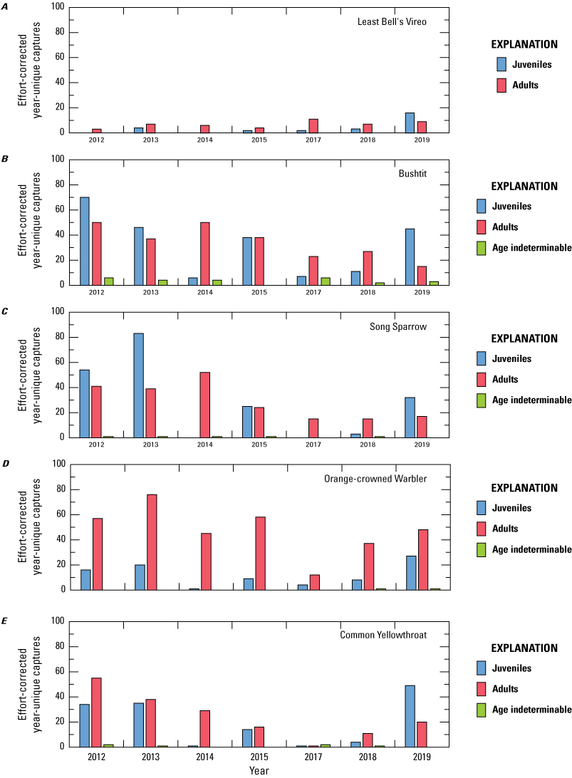
Annual variation in effort-corrected captures for five species that bred at Naval Outlying Landing Field, Imperial Beach, California, 2012‒19. Capture rates are divided into adults, juveniles, and birds of indeterminable age.
From 2012 to 2019, local population size, as measured by the effort-corrected number of adult captures, increased for Least Bell’s Vireo (Pearson’s r=0.69, P=0.09) and decreased for Bushtit (Pearson’s r=−0.90, P=0.01), Common Yellowthroats (Pearson’s r=−0.80, P=0.03), and Song Sparrows (Pearson’s r=−0.84, P=0.02; fig. 6). Orange-crowned Warblers (Pearson’s r=−0.58, P=0.17) had a near-significant negative population trend. All species except Least Bell’s Vireo exhibited a sharp decrease in captures in 2017.
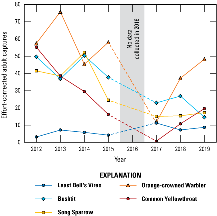
Adult population size for five bird species at Naval Outlying Landing Field, Imperial Beach, California, 2012–19. See appendix 1 for common and scientific names.
Climate Variables
All measures of precipitation (bio-year, early winter, and late winter) were highly variable during the operation of the station (figs. 7A‒C). Nevertheless, precipitation during the bio-year and during early winter was significantly greater during station operation than the historic mean (bio-year: Wilcoxon signed-rank test, W=74, P=0.11; early winter: Wilcoxon signed-rank test, W=43, P=0.01). Late winter precipitation did not deviate from the historical mean (two-sample t-test, t=0.46, P=0.65, df=24.9). Overall, precipitation was highest in 2020 and 2017 and lowest in 2014 and 2018.
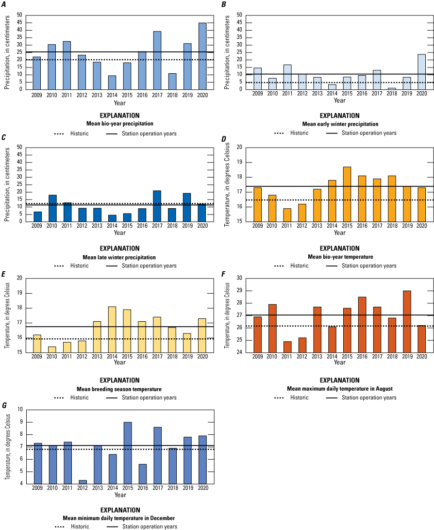
Annual variation in climate variables used in productivity and survival models. Bio-year was July 1[year x−1] to June 30[year x]. Early winter precipitation was October 1‒December 31, and late winter precipitation was January 1‒March 31. Climate variables were measured at Brown Field Municipal Airport (National Oceanic and Atmospheric Administration, 2022). Solid horizontal lines are means for the years the MAPS station was in operation (2009–20). Dotted lines are historical means (1945–46, 1954–61, and 1997–2008).
Although measures of temperature varied little during the operation of the station, mean bio-year temperature (Wilcoxon signed-rank test, W=44, P=0.002), mean temperature during the breeding season (March 1 through June 30; two-sample t-test, t=−2.43, P=0.02, df=26), and mean maximum daily temperature in August (two-sample t-test, t=−1.78, P=0.09, df=25.8) were significantly higher than the historical means (figs. 7D‒F). Mean minimum daily temperature in December did not deviate from the historical mean (two-sample t-test, t=−0.62, P=0.54, df=25.5; fig. 7G). Generally, the highest mean temperatures occurred between 2014 and 2019 and were significantly higher than historic averages (for all temperature variables except mean minimum daily temperature in December). The lowest mean temperatures were registered in 2011 and 2012 for all temperature variables and were higher than historic averages except for the mean minimum daily temperature in December.
Annual Productivity
Annual productivity was high for most focal species in 2010 and 2019 and low in 2014 and 2018 (fig. 8). Song Sparrow had the highest overall productivity (1.3±0.9 juveniles per adult; fig. 8E), and Least Bell’s Vireo had the lowest overall productivity (0.5±0.6 juveniles per adult; fig. 8A). Predictors of productivity were variable among species. Productivity for all species except Wrentit appeared to be driven by some measure of precipitation or temperature (tables 17, 18), although the constant model received strong support for all species except Song Sparrow and was the top model for Wrentit and Common Yellowthroat. The mean breeding season temperature was negatively associated with productivity of Least Bell’s Vireo, House Wren, Song Sparrow, Orange-crowned Warbler, and Common Yellowthroat (figs. 8A, 8D–G), although it varied by less than 3 degrees Celsius (°C; fig. 7E). Precipitation positively affected productivity in Least Bell’s Vireo and Bushtit. Productivity of Bushtits was positively associated with precipitation during the bio-year, with the highest Bushtit productivity occurring in 2020 following the bio-year with the most precipitation (45.0 centimeters, cm) and the lowest productivity for Bushtit occurring in 2014, concurrent with the bio-year with the least precipitation (9.4 cm; fig. 8B). Productivity of Least Bell’s Vireos was positively associated with late winter precipitation, with high productivity in 2010 and 2019 following the second (19.3 cm in 2019) and third (18.0 cm in 2010) highest accumulations of late winter precipitation; and low productivity in 2014 following the lowest accumulation of late winter precipitation (4.5 cm; fig. 8A). Late winter precipitation also was among the top models of productivity for Common Yellowthroat, with patterns similar to those for Least Bell’s Vireo; however, the relationship was not statistically significant (fig. 8G; 90-percent confidence intervals of the estimates crossed zero).
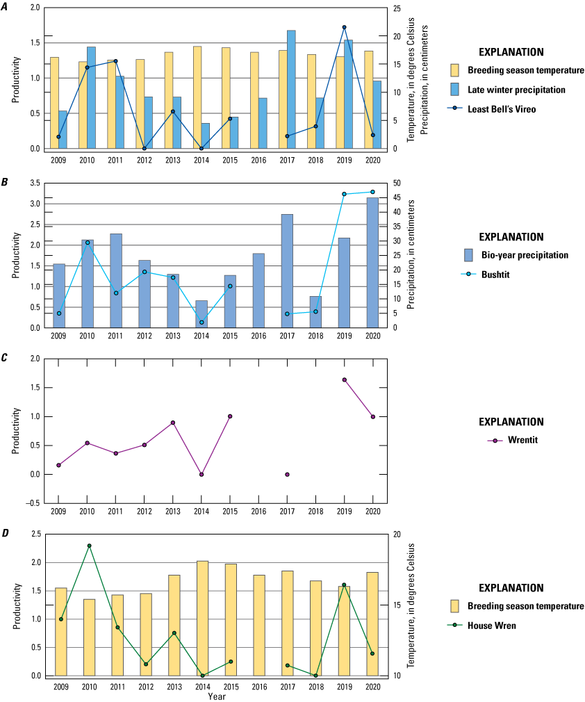
Annual productivity of seven bird species captured as a function of climate variables that influenced productivity according to top models. Climate variables were temperature (measured for the associated bio-year [July 1(year x−1) to June 30(year x)] and breeding season [March 1(year x) to June 30(year x)]), and precipitation (measured for bio-year [July 1(year x−1) to June 30(year x)], early winter [October 1(year x−1) to December 31(year x−1)], and late winter [January 1(year x) to March 31(year x)]) at Naval Outlying Landing Field, Imperial Beach, California, 2009–20. Productivity is calculated as the effort-corrected number of year-unique juveniles divided by the effort-corrected number of year-unique adults captured; this excludes the 2018 Wrentit productivity because unique-year captures were unusually low (5 individuals) and 80 percent (4/5) were juveniles, creating an artificially high productivity estimate for that year.
Table 17.
Multiple regression models for the effects of precipitation and temperature on breeding productivity of seven bird species captured at Naval Outlying Landing Field, Imperial Beach, California, 2009–20.[Models are ranked from most supported to least supported based on Akaike’s Information Criterion for small samples (AICc), the difference in AICc from this model and the top model (ΔAICc), and Akaike weights. The AICc is based on −2 x loge likelihood and the number of parameters in the model. Models with Akaike weights less than 0.05 are not presented. Precipitation and mean annual temperature were compiled for the July 1(year x−1) to June 30(year x) bio-year ending in the Monitoring Avian Productivity and Survivorship (MAPS) season. Mean temperature during the breeding season was compiled for March 1(year x) to June 30(year x)]
Table 18.
Summary of climate covariates that significantly affected productivity of seven bird species captured at Naval Outlying Landing Field, Imperial Beach, California, 2009–20.[. (dot), signifies no relationship; + (plus), indicates significant positive relationship; − (minus), indicates significant negative relationship]
Annual Survival
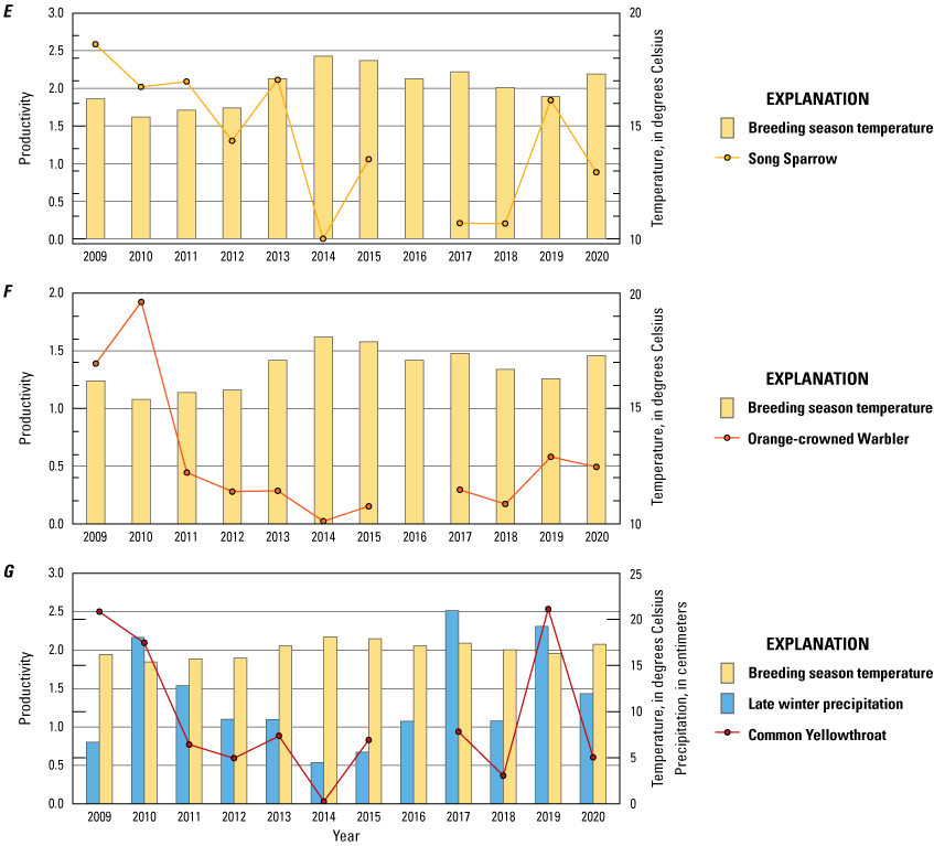
With some exceptions, adult annual survival was generally high from 2011 to 2012 (all species except Least Bell’s Vireo) and from 2018 to 2019 (all species except Bushtit and Orange-crowned Warbler; fig. 9). Otherwise, survival varied among years for all species, with no obvious annual patterns.
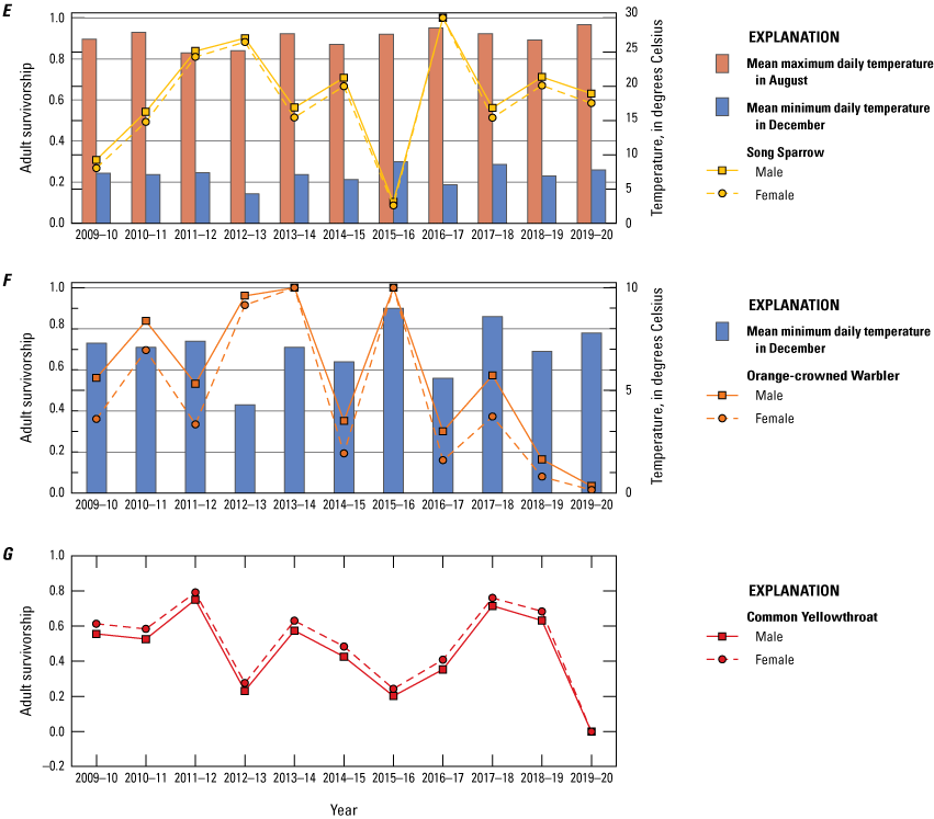
Adult annual survival (estimated by Program MARK) for seven bird species by sex and as a function of climate variables, according to top models. Climate variables were mean bio-year temperature (mean temperature for bio-year[year x−1 to year x]), mean maximum daily temperature in August[year x], mean minimum daily temperature in December[year x−1], bio-year precipitation (bio-year[year x−1 to year x]), early winter precipitation (October 1[year x−1] to December 31[year x−1]), and late winter precipitation (January 1[year x] to March 31[year x]) at Naval Outlying Landing Field, Imperial Beach, California, 2009–20. See appendix 1 for common and scientific names. Precipitation for migrant species (Least Bell’s Vireo) compiled for the bio-year[year x−2 to year x−1].
Climate factors that affected adult survival also varied among species (table 19). The only species significantly influenced by precipitation was Bushtit, which had lower annual survival with higher late winter precipitation (fig. 9B). Late winter precipitation was a significant predictor of Bushtit survival in both of the top-ranked models (table 20). Annual survival of five species was significantly influenced by temperature. In the top-ranked models, Bushtit survival was lower with lower mean minimum daily temperature in December and higher mean bio-year temperature (table 20). Top models showed that survival of Wrentit and Song Sparrow decreased with increasing mean maximum daily temperature in August (figs. 9C, 9E). Song Sparrow and Orange-crowned Warbler survival was lower with higher mean minimum daily temperature in December (figs. 9E, 9F), and House Wren survival was lower with higher mean bio-year temperature (fig. 9D; table 20).
Table 19.
Summary of climate covariates that significantly influence survival of seven bird species captured at Naval Outlying Landing Field, Imperial Beach, California, 2009–20.[. (dot), signifies no relationship; − (minus), indicates significant negative relationship; + (plus), indicates significant positive relationship]
Table 20.
Logistic regression models for the effects of sex, precipitation, and temperature on survival for seven bird species captured at Naval Outlying Landing Field, Imperial Beach, California, 2009–20.[Models are ranked from most supported to least supported based on Akaike’s Information Criterion for small samples (AICc), the difference in AICc from this model and the top model (ΔAICc), and Akaike weights. The AICc is based on −2 x loge likelihood and the number of parameters in the model. Models with Akaike weights less than 0.05 are not presented. Bio-year precipitation and mean annual temperature were compiled for the July 1(year x-1) to June 30(year x). Late winter precipitation was January 1(year x) to March 31(year x). Early winter precipitation was October 1(year x−1) to December 31(year x−1)]
Least Bell’s Vireo annual survival was not influenced by climate variables; however, it was significantly affected by sex (the highest-ranked model included only sex; table 20, fig. 9A). Male Least Bell’s Vireos had a higher annual survival rate (55 percent) than females (11 percent). Annual survival of Common Yellowthroats was not influenced by climate factors or by sex. The top model describing survival of adult Common Yellowthroat was the constant model. Although models containing sex, precipitation, and temperature variables were highly ranked, none of these variables significantly contributed to the models (table 20), indicating that sex and climate factors did not significantly affect survival (fig. 9G).
Predictors of Population Change
In multiple regression, changes in Bushtit, Song Sparrow, and Common Yellowthroat populations were influenced by annual survival and annual breeding productivity (table 21). The Bushtit population significantly increased with the combination of higher productivity during the previous year and higher annual survival. The Song Sparrow population increased with higher productivity during the previous year. The Common Yellowthroat population appeared to increase with increasing survival when in isolation (within the additive model, the survival parameter appears significant); however, the addition of productivity rendered the more complex model non-significant. Breeding productivity and annual survival did not appear to be strong predictors of population change for any of the other focal species.
Table 21.
Results of multiple regression analyses to predict population change (λ, the number of adults in yearx+1 /the number of adults in yearx) for seven bird species captured at Naval Outlying Landing Field, Imperial Beach, California, 2009–20.[Productivity estimates were corrected for effort within and between years. Population estimates were corrected for effort following methods in DeSante and others (2015). Abbreviations: P, probability; R2, coefficient of determination; R2P, probability associated with the coefficient of determination]
Discussion
Of the six most abundant species captured from 2014 to 2020 at NOLF, five were year-round residents and one was present only during migration (passage migrant). An additional nine species were abundant during at least 1 year, two that were year-round residents, two that were present only during winter, four that were migrants that bred at NOLF and wintered elsewhere, and one that was present only during migration. This range of resident and migrant species indicates that NOLF provides a diversity and abundance of resources necessary for breeding, wintering, and migration.
Similar to results from the prior data synthesis for 2009–13 (Lynn and others, 2015), seasonal capture rates for different species reflected differences in life history and breeding patterns. Peaks in capture rates for resident breeding species were driven by adult captures early in the breeding season and juvenile captures later in the season, representing fledging and juvenile dispersal events.
Starting in 2012, we began netting operations at the NOLF MAPS station in April, 1 month earlier than typical MAPS stations. This schedule allowed us to capture breeding data for species that begin breeding earlier than their northern and eastern conspecifics. Because of this expansion of the MAPS season, we documented juvenile Bushtits, California Thrashers, Song Sparrows, Orange-crowned Warblers, and Lesser Goldfinches (Spinus psaltria) in April in various years. Notably, no juvenile Song Sparrows were captured in April from 2012 to 2014 (per data found in this report and in Lynn and others [2015]). However, juvenile Song Sparrows were captured in April in 4 of the next 5 years (April 30, 2015, April 21, 2017, April 17, 2019, and April 24, 2020), indicating that the start of the Song Sparrow breeding season may be earlier than in the past. We did not see this pattern in any of the other species. The earlier commencement of Song Sparrow breeding at NOLF may be an effect of rising temperatures. Temperature was negatively associated with Song Sparrow productivity and survival, so the species may be shifting the start of its breeding season earlier, when the temperatures are cooler, resulting in increased productivity. Resident species, such as Song Sparrow, may have more phenotypic plasticity (defined as the ability of an organism to change in response to stimuli or inputs from the environment; West-Eberhard, 2008) and adjust timing based on local conditions, a strategy that is more challenging for migrant species. Lynn and others (2018) reported in a nearby study that multiple migratory species arrived later over time. The timing of bird migration evolved, allowing exploitation of the availability of food along the migration route; climate-caused shifts in phenology may adversely affect these species in the form of phenological mismatch (Cotton, 2003; Saino and others, 2011; Kellermann and van Riper, 2015).
Population trends were mixed for species captured at NOLF from 2012 to 2019. Least Bell’s Vireos increased but Bushtit, Common Yellowthroat, and Song Sparrow populations decreased. Common Yellowthroat and Song Sparrow populations also have declined since 1995 at the nearby De Luz MAPS station but were stable at the Santa Margarita MAPS station at Marine Corps Base Camp Pendleton (B. Kus, U.S. Geological Survey, unpub. data, 2021). Orange-crowned Warbler populations at NOLF were in decline until 2017 when they appeared to rebound. Populations of all species except Least Bell’s Vireo decreased dramatically in 2017. Effort-correction may partially explain low capture rate in 2017 (survey days were all longer than intended with the extra hours added during early afternoon when bird activity was reduced). However, the absolute number of captures in 2017 also was unusually low, driven primarily by the near absence of juvenile captures, despite high precipitation and high productivity in other areas of San Diego County (B. Kus, U.S. Geological Survey, unpub. data, 2021). This dip in breeding productivity is likely associated with a dramatic change in riparian habitat caused by infestation of the Tijuana River Valley by Kuroshio shot hole borer beetles (Euwallacea kuroshio) in 2015 (Boland, 2016). Adult beetles burrow into tree trunks, lay their eggs, and cultivate a Fusarium fungus which feeds the developing larvae. The Fusarium fungus damages or kills the tree, causing branch loss and collapse of tree trunks (University of California Agriculture and Natural Resources, 2019), a situation that was noticed in the Tijuana River Valley in late 2015 and early 2016 (Boland, 2016). Shot hole borer surveys documented infestation of approximately 70 percent of willow trees in winter 2015–16, 24 percent of which were dead as a result of infestation. The NOLF MAPS station was not operated in 2016, but by 2017, large stands of willows at the MAPS station had died or had been blown down as a result of weakened trunks. The destruction of woody trees that formed the riparian canopy likely had a strong, negative effect on riparian-nesting birds and resulted in low breeding productivity and low occupancy that year. Although Least Bell’s Vireo numbers declined in the highly infested riparian forests, they increased in neighboring riparian scrub that also was encompassed by the NOLF MAPS station (B. Kus, U.S. Geological Survey, unpub. data, 2022). Populations of Orange-crowned Warbler, Song Sparrow, and Common Yellowthroat began increasing again in 2018, concurrent with partial recovery of riparian vegetation in the Tijuana River Valley.
Productivity at NOLF was generally high in 2010 and 2019, following years with high precipitation, and low in 2014 and 2018, following years with low precipitation. Among the analyzed species in common with our nearby Santa Margarita MAPS station at Marine Corps Base Camp Pendleton (Least Bell's Vireo, Song Sparrow, Orange-crowned Warbler, and Common Yellowthroat), Song Sparrows had among the highest productivity and Least Bell’s Vireos had among the lowest productivity at both stations during the same period (B. Kus, U.S. Geological Survey, unpub. data, 2021). Adult survival appeared to be driven by a variety of parameters which were inconsistent among species. Similar to the Santa Margarita MAPS station at Marine Corps Base Camp Pendleton, Least Bell’s Vireo survival at NOLF was mostly influenced by sex: males had higher survival rates than females.
Drought has been found to negatively impact resource availability, primary productivity, and avian productivity and survival (Saracco and others, 2018). At NOLF, climate may have influenced productivity for all species except Wrentit and survival for all except Least Bell’s Vireo and Common Yellowthroat. Productivity was positively associated with precipitation, and both productivity and survival were negatively associated with temperature in most cases. Cox and others (2013) found that increasing daily maximum temperatures led to an increase in the rate of nest predation by snakes and birds. Higher temperatures increase disease transmission as well; West Nile Virus has been found to overwinter in southern California, and when winter temperatures exceed 14.3 °C, the virus replicates and transmits to avian hosts (Reisen and others, 2014). Although it varied by less than 3 °C , mean temperature during the breeding season was among the variables in the top models for 71 percent (5/7) of species, with temperature increases associated with reduced productivity in all five species. Similarly, temperature was negatively associated with survival of 71 percent (5/7) of species. Bushtit survival, in contrast, was more complicated. In the two top well-supported models, Bushtit survival was positively associated with mean low temperature in December but negatively associated with mean annual temperature, indicating that Bushtit survival was best in generally cool years with warm winters. With long-term temperature increases predicted by climate change models (0.8–2.5 °C in San Diego from 1970 to 2050; Messner and others, 2011), demographics of these species are likely to change, and increases in predation and disease are to be expected.
Several studies have found that winter precipitation influences productivity (Nott and others, 2002; Bolger and others, 2005; DeSante and others, 2005; Zarzycki, 2017; B. Kus, U.S. Geological Survey, unpub. data, 2019, 2021). Increased precipitation causes a rise in plant (Birtwistle, 2015) and arthropod abundance (Bolger and others, 2005), which increases fledging success and adult survival (Bolger and others, 2005). Results indicate that the relationship may be further influenced by the timing of winter precipitation (for example, whether it occurs early or late in the season). Productivity of Least Bell’s Vireo was higher with late winter precipitation, which is likely an effect of arthropod abundance boosting food availability during their breeding activities. Least Bell’s Vireo productivity increased with higher precipitation and lower breeding season temperatures. Bushtit was the only species for which survival rate was influenced by precipitation, with Bushtit survival decreasing with increasing precipitation in late winter.
Population size of three of the seven bird species was associated with either breeding productivity the previous year (Bushtit and Song Sparrow) or adult survival from the previous year (Bushtit and Common Yellowthroat). Song Sparrow and Bushtit populations were positively associated with increased breeding productivity during the previous year. Bushtit and Common Yellowthroat populations increased with increasing annual survival.
Whereas productivity and survivorship are ultimately important in explaining the life history of any organism, our analyses have shown precipitation and temperature to be important primary predictors for productivity and survival of the riparian bird species that we analyzed in our study area. However, the constant model for productivity received strong support for almost all species and was the top model for Wrentit and for productivity and survival of Common Yellowthroat, indicating that other, unexamined variables also may have a significant effect on these population parameters. With data from additional years, we can continue to develop our understanding of the relationships between climate, arrival dates, onset of nesting, phenological mismatch (Cotton, 2003; Saino and others, 2011; Kellermann and van Riper, 2015), habitat alteration, and the resulting demographic consequences for avian species that winter at, breed at, and migrate through NOLF. Building on these data by continuing the MAPS program at NOLF will help to elucidate the interacting contributions of productivity, survivorship, and climate to observed patterns in bird populations.
References Cited
Bartoń, K., 2020, MuMIn software package—Multi-model inference, version 1.43.17: CRAN, R Project, accessed February 16, 2022, at https://cran.r-project.org/web/packages/MuMIn/index.html.
Boland, J.M., 2016, The impact of an invasive ambrosia beetle on the riparian habitats of the Tijuana River Valley, California: PeerJ, v. 4, no. e2141, accessed February 14, 2022, at https://doi.org/10.7717/peerj.2141.
Bolger, D.T., Patten, M.A., and Bostock, D.C., 2005, Avian reproductive failure in response to an extreme climatic event: Oecologia, v. 142, p. 398–406. [Available at https://doi.org/10.1007/s00442-004-1734-9.]
California Department of Fish and Wildlife, 2021, Fully protected animals: California Department of Fish and Wildlife website, accessed November 15, 2021, at https://wildlife.ca.gov/Conservation/Fully-Protected#BIRDS.
California Department of Fish and Wildlife, 2023, State and federally listed endangered and threatened animals of California: California Department of Fish and Wildlife website, accessed June 15, 2023, at http://nrm.dfg.ca.gov/FileHandler.ashx?DocumentID=109405&inline.
Cotton, P.A., 2003, Avian migration phenology and global climate change: Proceedings of the National Academy of Sciences, v. 100, no. 21, p. 12219–12222. [Available at https://doi.org/10.1073/pnas.1930548100.]
Cox, W.A., Thompson, F.R., III, and Reidy, J.L., 2013, The effects of temperature on nest predation by mammals, birds, and snakes: The Auk, v. 130, no. 4, p. 784–790. [Available at https://doi.org/10.1525/auk.2013.13033.]
DeSante, D.F., Burton, K.M., Kaschube, D., Velez, P., Froehlich, D., and Albert, S., 2021, MAPS manual—2021 protocol—Instructions for the establishment and operation of constant-effort bird-banding stations as part of the Monitoring Avian Productivity and Survivorship (MAPS) Program: Petaluma, Calif., Institute for Bird Populations, 90 p., accessed December 13, 2021, at https://www.birdpop.org/docs/misc/MAPSManual21.pdf.
DeSante, D.F., Kaschube, D.R., and Saracco, J.F., 2015, Vital rates of North American landbirds: The Institute for Bird Populations website, accessed November 2, 2021, at https://www.VitalRatesOfNorthAmericanLandbirds.org.
DeSante, D.F., Nott, M.P., and Kaschube, D.R., 2005, Monitoring, modeling, and management—Why base avian management on vital rates and how should it be done? in Ralph, C.J., and Rich, T.D., eds., 2005, Bird conservation implementation and integration in the Americas—Proceedings of the Third International Partners in Flight Conference, March 20–24, 2002, Asilomar, Calif.: Albany, Calif., U.S. Department of Agriculture, Forest Service, Pacific Southwest Research Station, General Technical Report PSW-GTR-191, v. 2, p. 795–804.
Kellermann, J.L., and van Riper, C., III, 2015, Detecting mismatches of bird migration stopover and tree phenology in response to changing climate: Oecologia, v. 178, p. 1227–1238. [Available at https://doi.org/10.1007/s00442-015-3293-7.]
Lynn, S., Madden, M.C., Houston, A., and Kus, B.E., 2015, Monitoring Avian Productivity and Survivorship (MAPS) 5-year summary, Naval Outlying Landing Field, Imperial Beach, southwestern San Diego County, California, 2009–13: U.S. Geological Survey Open-File Report 2015–1035, 58 p., accessed February 7, 2022, at https://doi.org/10.3133/ofr20151035.
Lynn, S., Hall, K.A., Madden, M.C., and Kus, B.E., 2018, Monitoring breeding and migration of neotropical migratory birds at Naval Base Coronado, Remote Training Site, Warner Springs, San Diego County, California—5-year summary, 2013–17: U.S. Geological Survey Open-File Report 2018–1112, 98 p., accessed on December 13, 2021, at https://doi.org/10.3133/ofr20181112.
Messner, S., Miranda, S.C., Young, E., and Hedge, N., 2011, Climate change-related impacts in the San Diego region by 2050: Climatic Change, v. 109, no. 1, p. 505–531, accessed March 8, 2023, at https://link.springer.com/article/10.1007/s10584-011-0316-1. [Available at https://doi.org/10.1007/s10584-011-0316-1.]
National Oceanic and Atmospheric Administration, 2022, Climate data online—Dataset discovery: National Oceanic and Atmospheric Administration website, accessed February 1, 2022, at https://www.ncdc.noaa.gov/cdo-web/datasets#GSOM.
Nott, M.P., DeSante, D.F., Siegel, R.B., and Pyle, P., 2002, Influences of the El Niño/Southern Oscillation and the North Atlantic Oscillation on avian productivity in forests of the Pacific Northwest of North America: Global Ecology and Biogeography, v. 11, no. 4, p. 333–342. [Available at https://doi.org/10.1046/j.1466-822X.2002.00296.x.]
Pradel, R., 1996, Utilization of capture-mark-recapture for the study of recruitment and population growth rate: Biometrics, v. 52, no. 2, p. 703–709. [Available at https://doi.org/10.2307/2532908.]
R Core Team, 2022, R—A language and environment for statistical computing: Vienna, Austria, R Foundation for Statistical Computing website. [Available at https://www.R-project.org/.]
Saino, N., Ambrosini, R., Rubolini, D., von Hardenberg, J., Provenzale, A., Hüppop, K., Hüppop, O., Lehikoinen, A., Lehikoinen, E., Rainio, K., Romano, M., and Sokolov, L., 2011, Climate warming, ecological mismatch at arrival and population decline in migratory birds: Proceedings of the Royal Society of B, Biological Sciences, v. 278, no. 1707, p. 835–842. [Available at https://doi.org/10.1098/rspb.2010.1778.]
Saracco, J.F., Fettig, S.M., San Miguel, G.L., Mehlman, D.W., Thompson, B.E., and Albert, S.K., 2018, Avian demographic responses to drought and fire—A community‐level perspective: Ecological Applications, v. 28, no. 7, p. 1773–1781. [Available at https://doi.org/10.1002/eap.1751.]
Shuford, W.D., and Gardali, T.G., eds., 2008, California bird species of special concern—A ranked assessment of species, subspecies, and distinct populations of birds of immediate conservation concern in California—Studies of western birds, no.1: Sacramento, Calif., Western Field Ornithologists, California Department of Fish and Game, 65 p. [Available at https://www.contracosta.ca.gov/DocumentCenter/View/34166/Shuford-Gardali-2008-California-Bird-Species-of-Special-Concern-PDF.]
University of California Agriculture and Natural Resources, 2019, Distribution of PSHB/FD and KSHB/FD in California: Environmental Systems Research Institute (ESRI), accessed August 7, 2019, at https://ucanr.maps.arcgis.com/apps/Viewer/index.html?appid=3446e311c5bd434eabae98937f085c80.
U.S. Fish and Wildlife Service, 2021, Birds of conservation concern 2021: Falls Church, Va., U.S. Department of the Interior, U.S. Fish and Wildlife Service, accessed March 8, 2023, at https://fws.gov/media/birds-conservation-concern-2021pdf.
U.S. Navy, 2013, Final integrated natural resources management plan, Naval Base Coronado, California: U.S. Navy website, accessed February 28, 2023, at https://downloads.regulations.gov/FWS-R8-ES-2019-0113-0005/attachment_35.pdf.
West-Eberhard, M.J., 2008, Phenotypic plasticity, in Jørgensen, S.E., and Fath, B.D., eds., Encyclopedia of ecology: Academic Press, p. 2701–2707, accessed February 18, 2022, at https://www.sciencedirect.com/science/article/pii/B9780080454054008375. [Also available at https://doi.org/10.1016/B978-008045405-4.00837-5.]
White, G.C., and Burnham, K.P., 1999, Program MARK—Survival estimation from populations of marked animals: Bird Study, v. 46, p. S120–S139. [Available at https://doi.org/10.1080/00063659909477239.]
Appendix 1. Alpha Codes, Common Names, and Scientific Names for Species Captured and Observed, Naval Outlying Landing Field, Imperial Beach, California, 2014–20
Table 1.1.
Species captured at Naval Outlying Landing Field, Imperial Beach, California, 2014–20.[Special status: BCC-C, Bird of Conservation Concern, continental U.S.; BCC-R, Bird of Conservation Concern within the coastal California Bird Conservation Region; FE, listed as federally endangered; FT, listed as federally threatened (U.S. Fish and Wildlife Service, 2021); CA-SCC, listed as a species of special concern in California (Shuford and Gardali, 2008); CA-E, listed as endangered by the State of California; —, no data]
Table 1.2.
Species observed but not captured at Naval Outlying Landing Field, Imperial Beach, California, 2014–20.[Special status: BCC-C, Bird of Conservation Concern, continental U.S.; BCC-R, Bird of Conservation Concern within the coastal California Bird Conservation Region (U.S. Fish and Wildlife Service, 2021); CA-SCC, listed as a species of special concern in California (Shuford and Gardali, 2008); CA-FP, fully protected species by the State of California (California Department of Fish and Wildlife, 2023); —, no data]
Conversion Factors
Supplemental Information
Note to USGS users: Use of hectare (ha) as an alternative name for square hectometer (hm2) is restricted to the measurement of small land or water areas.
Abbreviations
AICc
Akaike’s Information Criterion for small sample sizes
DOD PIF
Department of Defense Partners in Flight
DOD
U.S. Department of Defense
IBP
Institute for Bird Populations
MAPS
Monitoring Avian Productivity and Survivorship
NASNI
Naval Air Station North Island
NOLF
Naval Outlying Landing Field
P
statistical probability that the result of a test was incorrect
PDT
Pacific Daylight Time
USFWS
U.S. Fish and Wildlife Service
USGS
U.S. Geological Survey
ΔAICc
difference in Akaike’s Information Criterion for sample sizes
λ
change in population size
For more information concerning the research in this report, contact the
Director, Western Ecological Research Center
U.S. Geological Survey
3020 State University Drive East
Sacramento, California 95819
https://www.usgs.gov/centers/werc
Publishing support provided by the U.S. Geological Survey
Science Publishing Network, Sacramento Publishing Service Center
Disclaimers
Any use of trade, firm, or product names is for descriptive purposes only and does not imply endorsement by the U.S. Government.
Although this information product, for the most part, is in the public domain, it also may contain copyrighted materials as noted in the text. Permission to reproduce copyrighted items must be secured from the copyright owner.
Suggested Citation
Lynn, S., Mendia, S., and Kus, B.E., 2023, Monitoring Avian Productivity and Survivorship (MAPS) 6-year summary, Naval Outlying Landing Field, Imperial Beach, southwestern San Diego County, California, 2014–20: U.S. Geological Survey Open-File Report 2023–1055, 68 p., https://doi.org/10.3133/ofr20231055.
ISSN: 2331-1258 (online)
Study Area
| Publication type | Report |
|---|---|
| Publication Subtype | USGS Numbered Series |
| Title | Monitoring Avian Productivity and Survivorship (MAPS) 6-year summary, Naval Outlying Landing Field, Imperial Beach, southwestern San Diego County, California, 2014–20 |
| Series title | Open-File Report |
| Series number | 2023-1055 |
| DOI | 10.3133/ofr20231055 |
| Publication Date | November 07, 2023 |
| Year Published | 2023 |
| Language | English |
| Publisher | U.S. Geological Survey |
| Publisher location | Reston, VA |
| Contributing office(s) | Western Ecological Research Center |
| Description | viii, 68 p. |
| Country | United States |
| State | California |
| County | San Diego County |
| Online Only (Y/N) | Y |