

Approaches for Using CMIP Projections in Climate Model Ensembles to Address the ‘Hot Model’ Problem
Links
- Document: Report (820 KB pdf) , HTML , XML
- Download citation as: RIS | Dublin Core
Acknowledgments
We would like to thank Levi Brekke of the Bureau of Reclamation, Jeff Lukas of Lukas Climate Research and Consulting, Robyn Niver of the U.S. Fish and Wildlife Service, and Amber Runyon of the National Park Service for their edits and comments on this report.
This research was funded by the U.S. Geological Survey (USGS). This research was also supported in part by an appointment to the USGS Research Participation Program administered by the Oak Ridge Institute for Science and Education (ORISE) through an interagency agreement between the U.S. Department of Energy (DOE) and the U.S. Department of the Interior (DOI). ORISE is managed by Oak Ridge Associated Universities (ORAU) under DOE.
Abstract
Several recent generation global-climate models were found to have anomalously high climate sensitivities and may not be useful for certain applications. Four approaches for developing ensembles of climate projections for applications that address this issue are:
-
1. Using an “all models” approach;
-
2. Screening using equilibrium climate sensitivity and (or) transient climate response;
-
3. Bayesian model averaging; and
-
4. Using global warming levels.
Advantages and disadvantages of each approach are described by using example applications to study the effects of climate change on an imaginary at-risk species. Choosing the right approach is dependent on the location, goals, and system focus of each application and the risk-tolerance and resource-management context.
Introduction
The purpose of this document is to provide information on approaches for developing ensembles of climate futures using global climate models (GCMs), available as part of the Coupled Model Intercomparison Project (CMIP). More information regarding CMIP can be found at Eyring and others, (2016). This guidance is intended for an audience of scientists and technical users, which include U.S. Geological Survey (USGS) Climate Adaptation Science Center partners who support resource management. The approaches that are discussed in this report account for climate sensitivity to greenhouse gas forcing in model-ensemble selection and working with CMIP data in a way that addresses some issues introduced by the anomalous “hot models” described below. This document does not include all possible model selection approaches since the criteria are often specific to user needs and applications.
Equilibrium climate sensitivity (ECS) and transient climate response (TCR) are closely related metrics of the Earth’s surface-warming response to additional greenhouse-gas concentrations in the atmosphere (refer to glossary for definition of terms). GCMs with relatively high ECS and TCR will project more warming, both globally and regionally, for a particular greenhouse gas-emissions scenario or future time period than those with relatively low ECS and TCR. As summarized in the Intergovernmental Panel on Climate Change (IPCC) Sixth Assessment Report (AR6) Working Group 1 Summary for Policy Makers (WG1 SPM), the scientific community has recently narrowed the estimated range in temperature for ECS and TCR. IPCC AR6 WG1 SPM A.4.4 (IPCC, 2021, p. 11) states that “based on multiple lines of evidence, the “very likely” range of equilibrium climate sensitivity is between 2 [degrees Celsius] °C (high confidence) and 5°C (medium confidence). The AR6-assessed best estimate is 3°C with a “likely” range of 2.5°C to 4°C (high confidence).”
IPCC AR6 WG1 Technical Summary (Arias and others, 2021, p. 93) adds
“There is a high level of agreement among the four main lines of evidence listed above (Figure TS.16b), and altogether it is virtually certain that ECS is larger than 1.5°C, but currently it is not possible to rule out ECS values above 5°C. Therefore, the 5°C upper end of the very likely range is assessed with medium confidence and the other bounds with high confidence.”
Figure 1 shows how assessments of ECS have evolved through IPCC reports. Assessment of this narrowed range of ECS and TCR in IPCC AR6 is based on multiple lines of evidence, which includes new information on physical processes, comparison with the observations from the instrumental record and paleoclimate studies, and emergent constraints studies, so models with ECS and TCR outside of these ranges may be considered less physically plausible with respect to projected warming and its effects. As shown in appendix 1, a sizeable fraction of the GCMs used in CMIP version 6 (CMIP6) have ECS and (or) TCR outside of these ranges. Although some GCMs used in the previous CMIP version 5 (CMIP5) are also outside those ranges, the proportion is much lower than GCMs for CMIP6. The high ECS and TCR in CMIP6 is due primarily to model physics and parameterization associated with cloud processes (Dong and others, 2020; Zelinka and others, 2020; Schuddeboom and McDonald, 2021; Smith and others, 2021; Wang and others, 2021; Lutsko and others, 2022).
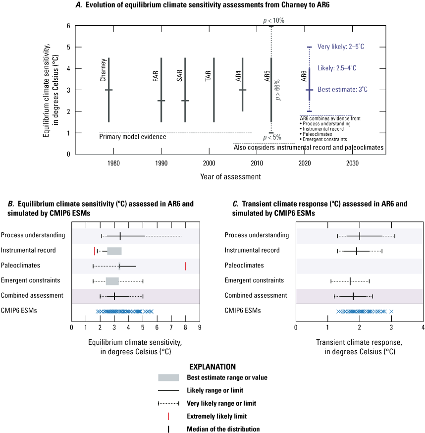
Models showing A, evolution of equilibrium climate sensitivity (ECS) assessments from the Charney Report (a precursor to IPCC Assessment Reports) through a succession of Intergovernmental Panel on Climate Change (IPCC) Assessment Reports to Sixth Assessment Report (AR6), and lines of evidence and combined assessment for B, ECS and C, Transient climate response (TCR) in AR6. This figure is adapted from Arias and others (2021) Figure TS.16.
There are many advantages to using GCMs from CMIP6, as these models include improved representations of physical, chemical, and biological processes at the global scale and generally have higher spatial resolution than previous versions (IPCC, 2021). Furthermore, consideration of an ensemble of model projections is advised since no single model performs best in every region or for every variable of interest, and often the improvements in CMIP6 are application-specific. The use of CMIP6 projections for resource-management applications will grow increasingly in coming years as downscaled datasets, hydrological projections, and associated decision-support tools become available. As of August 2023, most downscaled-climate projections (including derived variables) and decision-support tools are available only for CMIP5 and are therefore useful for many resource-management applications until similar CMIP6 products become available for comparison.
Whenever possible, those wanting to use output from GCMs (and projections downscaled from GCMs) should use multiple-emissions scenarios and multiple GCMs for each scenario to capture a range of possible future conditions (Department of the Interior, 2023), with the understanding that the choice of scenarios is related to the sensitivity and risk profile of the decision. There is extensive literature on model-selection approaches for different purposes (Brekke and others, 2008; Snover and others, 2013; Dubrovksy and others, 2014; Cannon, 2015; Chen and others, 2016; Ruane and McDermid, 2017; Herger and others, 2018; Ross and Najjar, 2019; Rangwala and others, 2021; Mahony and others, 2022; Miller and others, 2022; Wootten and others, 2023), a review of which is beyond the scope of this report.
GCM skill, bias, or performance for single metrics should not generally be considered as a basis for model selection since models will have varying performance by variable and region, and accuracy in reproducing one variable may not be evidence of overall systemic reliability of the model (Knutti 2010; Weigel and others, 2010; Mote and others, 2011; Herger and others, 2019). However, screening by global constraints (such as ECS and TCR) may be appropriate for selection of GCMs as part of an ensemble for analysis. There are a variety of approaches for selecting and (or) weighting the GCMs used in an ensemble based on an understanding of ECS and (or) TCR. Here, we describe several of these approaches that may be considered to develop an ensemble of models to explore the effects of climate change on natural and cultural resources. The preferred approach will be dependent on the user application and implications for resource-management context, so no single approach or combination of approaches is recommended for all situations.
Approaches for GCM Selection and Weighting
All Models Approach
Retaining all models for the analysis ensemble has been a common approach (when analytically feasible) since the IPCC Fourth Assessment Report. In this approach, all GCM projections are considered equally plausible realizations of future conditions (Bureau of Reclamation, 2011; Lawrence and others, 2021) for any given emissions scenario. Retaining the entire set of models allows for the inclusion of the full range of simulated conditions for all available variables. This approach is consistent with more risk-averse decision environments, such as when an end-user is more concerned about the effects associated with low-probability outcomes. However, the retention of all models should be accompanied by a note that the decision of including models with high ECS and TCR may lead to an increased consideration of potentially implausible high future risks for any scenario.
ECS and TCR Screening
Some applications of climate models may allow for use of projection averages or ensemble means, but most impact modeling (hydrologic, land use, ecological, carbon cycling) and dynamical downscaling require the use of individual-model realizations as the climate input. Given the scientific advancement summarized above from IPCC AR6 WG1, screening of models using ECS and (or) TCR ranges provide one viable approach for limiting the GCMs included for impact studies and planning. In some cases, where computational, analytical, and practical constraints demand the selection of a small subset of GCMs for further analysis, ECS and (or) TCR screening can also be used in combination with other selection approaches.
Screening by ECS and (or) TCR disregards models outside the “likely” (66 percent chance range; ECS: 2.5°C–4°C, TCR: 1.4°C–2.2°C) or “very likely” (90 percent chance range; ECS: 2°C–5°C, TCR: 1.2°C–2.4°C), based on the IPCC AR6 WG1 assessment (app. 1). Exclusion of models outside the range of “likely” ECS has been suggested as a viable approach in some studies (Tokarska and others, 2020; Ribes and others, 2021; Hausfather and others, 2022). Selection based on the ECS range of 2.5–4°C eliminates 60 percent of CMIP6 models. Alternatively, Hausfather and others (2022) suggests using TCR ranges inside the “likely” (66 percent chance) range of 1.4–2.2°C for model selection because this approach only excludes 40 percent of CMIP6 models.
The choice of using ECS or TCR ranges for screening depends on user application and consideration of risk. A risk-averse approach may involve adopting the “very likely” ECS range (as opposed to the “likely” range). However, model selection that is based exclusively on ECS and (or) TCR has the potential to remove valuable information (Hausfather and others, 2022), which includes plausible extremes, precipitation variability, and other reasonable ranges for patterns of natural variability (box TS.3 in Arias and others, 2021). Although regional temperatures are usually highly correlated with ECS and TCR, this approach may not be appropriate in some regions that have other complex dynamics, which include areas affected by sea-ice dynamics, convective precipitation, onshore wind, monsoons, and large lakes with complex moisture and heat fluxes (Douglas and Atwood, 2022; Schneider and others, 2022). Users may wish to consider models outside the upper range of ECS and TCR when “low-likelihood, high-warming” scenarios have a major effect on the resource or system being considered (Arias and others, 2021).
Bayesian Model Averaging
An alternative approach to model selection is to retain the full ensemble of climate models and apply weights to each model that reflect the best available information on their accuracy. There are many different weighting approaches that could be used, including those used in the National Climate Assessments (Basile and others, 2023) that have accounted for model skill and independence. One approach, Bayesian Model Averaging (BMA; Raftery and others, 2005; Terando and others, 2012; Massoud and others, 2023), is appealing because model weights and uncertainty are estimated by maximizing a likelihood function that is consistent with scientific understanding of the true state of nature (or the climate system). In this case, the posterior distribution of model likelihoods (the weights) and the uncertainty estimates around those weights are based on thousands of different weighted combinations of ECS values from the ensemble members, which are then compared to the “true” distribution. Here, “truth” is the estimated ECS distribution provided by the IPCC Sixth Assessment Report (Forster and others, 2021), which does not use CMIP6 model outputs to attain the assessed value but rather represents an independent ECS estimate. After sampling thousands of combinations, the most optimal sets of model weights are extracted and used for post-processing. This avoids having to reject any models that are considered outside of the “likely” range of ECS, since all models may appear in any given set of weights. The individual model weights from Massoud and others (2023) are provided in appendix 1.
An advantage of using BMA is that information from models outside of the IPCC-assessed ECS-likelihood range are not discarded from the analysis—just given less (sometimes much less) weight. The resulting weighted ensemble of models is most consistent with current scientific understanding of the temperature sensitivity of Earth’s climate system. An advantage of using the BMA approach is that a fully probabilistic distribution of the “ensemble of opportunity” that represents the CMIP6 output is possible. This can provide not only a better representation of our state of knowledge about how the climate system works (such as the weights), but also a more formalized and faithful representation of our uncertainty about the current state of climate knowledge.
The disadvantage of this approach is the complexity required to apply the BMA weights through the entirety of an application or impact analysis. Transforming model outputs into a probabilistic projection should only be done at the end of the analysis. For example, if using this approach in a context where downscaled climate-model outputs are driving an ecosystem-process model to inform a resource-management decision, the transformation of model outputs to a probabilistic projection should only be performed at the end of the process after the ecosystem-model outputs are produced. Although this appropriately weights the climate input to the ecosystem-process model, the resulting averaging produces a weighted-mean-ecosystem response and masks individual model-simulated effects, which is an important consideration for scenario-planning or risk-averse applications. Furthermore, if the ensemble size of downscaled-climate models is smaller than the full set of earth system models for which BMA weights are available, the new set of weights and uncertainty estimates would need to be re-normalized to reflect the reduced model set. There is no single standard method for weighting, and methods other than those from Massoud and others (2023) may also be appropriate. Similarly, one could derive their own weighting method, but this is complex and requires rigorous calculations and peer reviews.
Global Warming Levels
Finally, some applications may benefit from the use of global warming levels (GWLs) to depict localized patterns of climate change associated with different amounts of average global surface-temperature warming. In 2018, the IPCC published a report that explores the effects of warming of 1.5oC and 2.0oC, which enables us to consider warmer futures without the explicit consideration of when those futures may occur (Hoegh-Guldberg and others, 2018). For example, the local-temperature response to a global-warming level of 3°C will be roughly the same if that amount of warming is reached in 75 years or 100 years. This approach can be similarly applied in the context of resource-management consideration. The advantage of this approach is that the challenges associated with very high ECS values in some members of the CMIP6 ensemble are avoided by removing the time component. This is done by combining results from the entire ensemble across all available scenarios at different levels of global warming (for example, 2°C, 3°C, and 4°C warming), irrespective of when that amount of global warming is projected to occur in individual ensemble members. The primary disadvantage is that this approach will not work for applications that require a time dimension for analysis (such as sea-level-rise planning). Some physical variables (such as sea-level rise) will have a slow response to the GWL, making it more difficult to accurately calculate the associated local-response pattern. In addition, downscaled projections for GWL periods are not commonly available for CMIP6 and are limited for CMIP5, so users of this approach would need to analyze the GCM output globally for a range of future time periods and build an ensemble of downscaled projections based on each GCM’s mean global temperature. More information can be found at IPCC–WG1, 2021. Refer to table 1 for more information.
Table 1.
Summary of advantages and disadvantages associated with the various approaches of developing ensembles of climate futures using global climate models.[ECS and TCR, equilibrium climate sensitivity/transient climate response; BMA, Bayesian model averaging; GWL, global warming levels]
| Approach | Advantages | Disadvantages |
|---|---|---|
| All models | • Retains all available information. • Simplest method. • Lower technical skill required for application. |
• Analytically intensive for many studies that require impact modeling. • May include less plausible projections based on ECS and TCR. |
| ECS and TCR screening | • Lower technical skill required for application. • Based on the current best understanding of climate sensitivity. • Generates a smaller ensemble for impact modeling. • Can be used in combination with other selection methods. |
• May remove information on other variables (for example, plausible extremes,
precipitation variability). • May not be appropriate for regions with other complex dynamics (for example, sea ice, monsoon, onshore wind). |
| BMA | • Higher technical skill required for application; lowered by using published
weights (Massoud and others, 2023). • Addresses some aspects of ECS and TCR exceedance without model selection. |
• Cannot create a smaller ensemble of models for use in impact studies. • Application of weighting approaches can be complicated, especially to non-numeric output (such as maps). • Interpretation can be complicated in scenario-planning or risk-averse applications. |
| GWL | • Addresses most aspects of ECS and TCR exceedance without model selection. • Non-committal to a specific future time horizon or emissions scenario. |
• Cannot create a smaller ensemble of models for use in impact studies. • Higher technical skill required for application, so more guidance, data and applications are required for widespread use. • Not useful in studies where the timing of effects of climate change is important. |
Example: The Imaginary Golden-billed Raptor
To illustrate the application of these approaches, this section provides an example of how each approach might be considered as part of a climate risk assessment for an imaginary at-risk species—the golden-billed raptor. In this scenario, the golden-billed raptor is a charismatic, migratory bird beloved by the American public. The raptor overwinters in the south-central United States and spends its summers along the southern shores of Lake Superior. This imaginary bird has physiological limits and is threatened by extreme high temperatures. Its critical habitat and food source has narrow requirements for temperature, precipitation, and it needs exceptionally sunny conditions. In this scenario, there exists a species model that adequately describes and captures how the golden-billed raptor and its critical habitat change, and this model has been validated using 30 years of climate and species data. We imagine that resource-management partners will want to understand the effects of climate change to this species over the next 80 years.
Using an “all models” approach, one would use appropriately downscaled CMIP6 GCM projections as an input to the species model for multiple-emissions scenarios and analyze the species-model output averaged in 30-year overlapping blocks between 2020 and 2100. In this approach, the species model illustrates a range of potential effects from each scenario. This is consistent with how the model was applied previously using CMIP5. Using CMIP6, one should also explicitly acknowledge and consider how the GCMs with ECS outside the “likely” range might affect the species-model output. If the species model shows little or no difference between outputs based on GCMs inside and outside the “ECS-likely” range, then there may be little risk in including these “hot models” for this application and region; however, if the species model shows substantial differences, then further analysis or consideration may be needed given the risks of extinction for a charismatic bird with high national visibility. Additionally, depending on the computational complexity of the species model and the time and expertise available, utilizing all available model projections may not be feasible. In that case, a more limited ensemble generated through ECS and TCR screening may be more appropriate to implement.
If an “ECS and TCR screening” approach is being used to limit the ensemble, one would choose to incorporate into our species model only those GCM projections with ECS and TCR within the “likely” IPCC range, but otherwise follow the same analysis methodology as used in the first application example. This reduces the number of downscaled GCMs used as input to the species model by 60 percent, which makes for a simpler analysis, but is still consistent with the Department of the Interior policy for using an ensemble of models and a reasonable scientific basis on which models can be excluded from the species analysis. Using this approach, the species model-output range would be narrower as compared to the “all models” approach and thus would explain a narrower range of plausible future effects to the species. Whereas ECS is highly correlated with the temperatures observed at this bird’s summer and winter habitat, it is not highly correlated with changes in precipitation or cloud cover in these locations, so one must consider if the species model is adequate to fully capture changes to its habitat with a more limited number of GCMs as compared to the other approaches. Moreover, we must consider if the resulting range of effects adequately reflects the true range given the importance of this bird to the people living in the United States.
If one wanted to use a BMA approach, we would follow the same steps as the “all models” approach and then apply the BMA weights from Massoud and others (2023) to the resulting species-model output. This approach has the advantage of providing a full ensemble of species impacts informed by each GCM’s ECS. Interpretation of individual species model outputs can be difficult because the BMA weights represent confidence in the output, not a specific numerical value (such as the probability of extinction or magnitude of habitat loss). Rather, the final weighted ensemble collectively captures scientific confidence in the GCM’s ability to simulate temperatures. As with the ECS and TCR screening approach, the sensitivity of the resulting species model to changes in precipitation and cloud cover may be incorrectly weighted since ECS and TCR are only highly correlated with regional temperatures.
Using a GWL approach, we would instead ask questions such as “If the Earth were 2.0°C warmer, what would be the effects to this bird?” We would then use IPCC AR6 WG1 list of years when the GCM mean global temperature was approximately 2.0°C in each model (IPCC–WG1, 2021). From these global-climate simulations, we would select the corresponding downscaled simulations for our regions of interest (or create these downscaled simulations if they did not already exist). We would then use those downscaled simulations as an input to our species-impact model and analyze the results. With this approach, there is no concern that ECS is not related to local precipitation or cloud cover. It also would not matter what the ECS is for any of the GCMs for this case because we are more interested in the regional climate (and the associated effects on this species) resulting from an Earth simulation that is 2.0°C warmer and not the background carbon dioxide (CO2) levels. However, using this approach would not allow us to consider when, over the next 100 years, an unacceptable risk of extinction may occur, as this approach does not allow for consideration of time.
Conclusion
This document offers several approaches for using global climate models (GCMs) in an ensemble of climate projections with the purpose of assisting the technical experts that support resource management. For all approaches, the use of a large ensemble of climate projections, whether centered around a time-period or global-warming level, is always recommended. Choosing the right approach is highly dependent on the location, goals, and system focus of each application and the risk-tolerance and resource-management context. No universal recommendation is being made here on which approach is most appropriate, as each approach has their unique advantages and disadvantages. Ultimately, selection of a method can be challenging and may warrant consultation with a climate-model expert.
References Cited
Arias, P.A., Bellouin, N., Coppola, E., Jones, R.G., Krinner, G., Marotzke, J., Naik, V., Palmer, M.D., Plattner, G.-K., Rogelj, J., Rojas, M., Sillmann, J., Storelvmo, T., Thorne, P.W., Trewin, B., Achuta Rao, K., Adhikary, B., Allan, R.P., Armour, K., Bala, G., Barimalala, R., Berger, S., Canadell, J.G., Cassou, C., Cherchi, A., Collins, W., Collins, W.D., Connors, S.L., Corti, S., Cruz, F., Dentener, F.J., Dereczynski, C., Di Luca, A., Diongue Niang, A., Doblas-Reyes, F.J., Dosio, A., Douville, H., Engelbrecht, F., Eyring, V., Fischer, E., Forster, P., Fox-Kemper, B., Fuglestvedt, J.S., Fyfe, J.C., Gillett, N.P., Goldfarb, L., Gorodetskaya, I., Gutierrez, J.M., Hamdi, R., Hawkins, E., Hewitt, H.T., Hope, P., Islam, A.S., Jones, C., Kaufman, D.S., Kopp, R.E., Kosaka, Y., Kossin, J., Krakovska, S., Lee, J.-Y., Li, J., Mauritsen, T., Maycock, T.K., Meinshausen, M., Min, S.-K., Monteiro, P.M.S., Ngo-Duc, T., Otto, F., Pinto, I., Pirani, A., Raghavan, K., Ranasinghe, R., Ruane, A.C., Ruiz, L., Sallée, J.-B., Samset, B.H., Sathyendranath, S., Seneviratne, S.I., Sörensson, A.A., Szopa, S., Takayabu, I., Tréguier, A.-M., van den Hurk, B., Vautard, R., von Schuckmann, K., Zaehle, S., Zhang, X., and Zickfeld, K., 2021, Technical summary in Masson-Delmotte, V., Zhai, P., Pirani, A., Connors, S.L., Péan, C., Berger, S., Caud, N., Chen, Y., Goldfarb, L., Gomis, M.I., Huang, M., Leitzell, K., Lonnoy, E., Matthews, J.B.R., Maycock, T.K., Waterfield, T., Yelekçi, O., Yu, R., and Zhou, B., eds., Climate change 2021—The physical science basis—Working group I contribution to the sixth assessment report of the intergovernmental panel on climate change: Cambridge and New York City, Cambridge University Press, p. 33–144. [Also available at https://doi.org/10.1017/9781009157896.002.]
Basile, S., Crimmins, A.R., Avery, C.W., Hamlington, B.D., and Kunkel, K.E., 2023, Appendix 3, scenarios and datasets in Crimmins, A.R., Avery, C.W., Easterling, D.R., Kunkel, B.C., Stewart, B.C., Maycock, T.K., eds., Fifth national climate assessment: U.S. Global Change Research Program, Washington, D.C. [Also available at https://doi.org/10.7930/NCA5.2023.A3.]
Brekke, L.D., Dettinger, M.D., Maurer, E.P., and Anderson, M., 2008, Significance of model credibility in estimating climate projection distributions for regional hydroclimatological risk assessments: Climatic Change, v. 89, p. 371–394 [Also available at https://doi.org/10.1007/s10584-007-9388-3.]
Bureau of Reclamation, 2011, West-wide climate risk assessments—Bias-corrected and spatially downscaled surface water projections: Bureau of Reclamation Water and Environmental Resources Division Technical Memorandum No. 86-68210-2011-01, 138 p. [Also available at https://www.usbr.gov/watersmart/docs/west-wide-climate-risk-assessments.pdf.]
Cannon, A.J., 2015, Selecting GCM scenarios that span the range of changes in a multimodel ensemble—Application to CMIP5 climate extremes indices: Journal of Climate, v. 28, no. 3, p. 1260–1267. [Also available at https://doi.org/10.1175/JCLI-D-14-00636.1.]
Chen, J., Brissette, F.P., and Lucas-Picher, P., 2016, Transferability of optimally-selected climate models in the quantification of climate change impacts on hydrology: Climate Dynamics, v. 47, p. 3359–3372. [Also available at https://doi.org/10.1007/s00382-016-3030-x.]
Department of the Interior, 2023, Part 526—Climate change science in Chapter 1—Applying climate change science of Department of Interior Departmental Manual: Office of Policy Analysis, 7 p. [Also available at https://www.doi.gov/sites/doi.gov/files/elips/documents/526-dm-1_1.pdf.]
Dong, Y., Armour, K.C., Zelinka, M.D., Proistosescu, C., Battisti, D.S., Zhou, C., and Andrews, T., 2020, Intermodel spread in the pattern effect and its contribution to climate sensitivity in CMIP5 and CMIP6 models: Journal of Climate, v. 33, no. 18, p. 7755–7775.[Also available at https://doi.org/10.1175/JCLI-D-19-1011.1.]
Douglas, D.C., and Atwood, T.C., 2022, Comparisons of coupled model intercomparison project phase 5 (CMIP5) and coupled model intercomparison project phase 6 (CMIP6) sea-ice projections in polar bear (Ursus maritimus) ecoregions during the 21st century: U.S. Geological Survey Open-File Report 2022–1062, 27 p., accessed August 2023 at https://doi.org/10.3133/ofr20221062.]
Dubrovsky, M., Trnka, M., Holman, I.P., Svobodova, E., and Harrison, P.A., 2014, Developing a reduced-form ensemble of climate change scenarios for Europe and its application to selected impact indicators: Climatic Change, v. 128, p. 169–186. [Also available at https://doi.org/10.1007/s10584-014-1297-7.]
Eyring, V., Bony, S., Meehl, G.A., Senior, C.A., Stevens, B., Stouffer, R.J., and Taylor, K.E., 2016, Overview of the coupled model intercomparison project phase 6 (CMIP6) experimental design and organization: Geoscientific Model Development, v. 9, no. 5, p. 1937–1958. [Also available at https://doi.org/10.5194/gmd-9-1937-2016.]
Forster, P., Storelvmo, T., Armour, K., Collins, W., Dufresne, J.-L., Frame, D., Lunt, D.J., Mauritsen, T., Palmer, M.D., Watanabe, M., Wild, M., and Zhang, H., 2021, The Earth’s energy budget, climate feedbacks, and climate sensitivity, chap. 7 of Masson-Delmotte, V., Zhai, P., Pirani, A., Connors, S.L., Péan, C., Berger, S., Caud, N., Chen, Y., Goldfarb, L., Gomis, M.I., Huang, M., Leitzell, K., Lonnoy, E., Matthews, J.B.R., Maycock, T.K., Waterfield, T., Yelekçi, O., Yu, R., and Zhou, B., eds., Climate change 2021—The physical science basis—Contribution of working group I to the sixth assessment report of the intergovernmental panel on climate change: Cambridge and New York City, Cambridge University Press, p. 923–1054. [Also available at https://doi.org/10.1017/9781009157896.009.]
Hausfather, Z., Marvel, K., Schmidt, G.A., Nielsen-Gammon, J.W., and Zelinka, M., 2022, Climate simulations—Recognize the ‘hot model’ problem: Nature, v. 605, p. 26–29. [Also available at https://doi.org/10.1038/d41586-022-01192-2.]
Herger, N., Abramowitz, G., Knutti, R., Angélil, O., Lehmann, K., and Sanderson, B.M., 2018, Selecting a climate model subset to optimise [sic] key ensemble properties: Earth System Dynamics: ESD, v. 9, no. 1, p. 135–151. [Also available at https://doi.org/10.5194/esd-9-135-2018.]
Herger, N., Abramowitz, G., Sherwood, S., Knutti, R., Angelil, O., and Sisson, S.A., 2019, Ensemble optimisation [sic], multiple constraints and overconfidence—A case study with future Australian precipitation change: Climate Dynamics, v. 53, p. 1581–1596. [Also available at https://doi.org/10.1007/s00382-019-04690-8.]
Hoegh-Guldberg, O., Jacob, D., Taylor, M., Bindi, M., Brown, S., Camilloni, I., Diedhiou, A., Djalante, R., Ebi, K.L., Engelbrecht, F., Guiot, J., Hijioka, Y., Mehrotra, S., Payne, A., Seneviratne, S.I., Thomas, A., Warren, R., and Zhou, G., 2018, Impacts of 1.5°C global warming on natural and human systems, chap. 3 of Masson-Delmotte, V., Zhai, P., Pörtner, H.-O., Roberts, D., Skea, J., Shukla, P.R., Pirani, A., Moufouma-Okia, W., Péan, C., Pidcock, R., Connors, S., Matthews, J.B.R., Chen, Y., Zhou, X., Gomis, M.I., Lonnoy, E., Maycock, T., Tignor, M., and Waterfield T., eds., Global warming of 1.5°C—An IPCC special report on the impacts of global warming of 1.5°C above pre-industrial levels and related global greenhouse gas emission pathways, in the context of strengthening the global response to the threat of climate change, sustainable development, and efforts to eradicate poverty: Cambridge and New York City, Cambridge University Press, p. 175–312. [Also available at https://doi.org/10.1017/9781009157940.005.]
IPCC, 2021, Summary for policymakers, in Masson-Delmotte, V., Zhai, P., Pirani, A., Connors, S.L., Péan, C., Berger, S., Caud, N., Chen, Y., Goldfarb, L., Gomis, M.I., Huang, M., Leitzell, K., Lonnoy, E., Matthews, J.B.R., Maycock, T.K., Waterfield, T., Yelekçi, O., Yu, R., and Zhou, B., eds.: Climate change 2021—The physical science basis—Contribution of working group I to the sixth assessment report of the intergovernmental panel on climate change: Cambridge and New York City, Cambridge University Press, p. 3–32. [Also available at https://doi.org/10.1017/9781009157896.001.]
IPCC–WG1, 2021, Global warming levels: GitHub website, accessed August 2023 at https://github.com/IPCC-WG1/Atlas/tree/main/warming-levels.
Knutti, R., 2010, The end of model democracy? An editorial comment: Climatic Change, v. 102, p. 395–404. [Also available at https://doi.org/10.1007/s10584-010-9800-2.]
Lawrence, D.J., Runyon, A.N., Gross, J.E., Schuurman, G.W., Miller, B.W., 2021, Divergent, plausible, and relevant climate futures for near- and long-term resource planning: Climatic Change, v. 167, no. 38, 20 p. [Also available at https://doi.org/10.1007/s10584-021-03169-y.]
Lutsko, N.J., Luongo, M.T., Wall, C.J., and Myers, T.A., 2022, Correlation between cloud adjustments and cloud feedbacks responsible for larger range of climate sensitivities in CMIP6: Journal of Geophysical Research Atmospheres, v. 127, no. 23. [Also available at https://doi.org/10.1029/2022JD037486.]
Mahony, C.R., Wang, T., Hamann, A., and Cannon, A.J., 2022, A global climate model ensemble for downscaled monthly climate normals over North America: International Journal of Climatology, v. 42, no. 11, p. 5871–5891. [Also available at https://doi.org/10.1002/joc.7566.]
Massoud, E.C., Lee, H.K, Terando, A., and Wehner, M., 2023, Bayesian weighting of climate models based on climate sensitivity: Communications Earth & Environment, v. 4, no. 365, 8 p. [Also available at https://doi.org/10.1038/s43247-023-01009-8.]
Meehl, G.A., Senior, C.A., Eyring, V., Flato, G., Lamarque, J.-F, Stouffer, R.J., Taylor, K.E., and Schlund, M., 2020, Context for interpreting equilibrium climate sensitivity and transient climate response from the CMIP6 Earth system models: Science Advances, v. 6, no. 26, 10 p. [Also available at https://doi.org/10.1126/sciadv.aba1981]
Miller, B.W., Schuurman, G.W., Symstad, A.J., Runyon, A.N., and Robb, B.C., 2022, Conservation under uncertainty—Innovations in participatory climate change scenario planning from U.S. national parks: Conservation Science and Practice, v. 4, no. 3, 15 p. [Also available at https://doi.org/10.1111/csp2.12633]
Möller, V., van Diemen, R., Matthews, J.B.R., Méndez, C., Semenov, S., Fuglestvedt, J.S., Reisinger, A., eds., 2022, Glossary, in Pörtner, H.-O., Roberts, D.C., Tignor, M., Poloczanska, E.S., Mintenbeck, K., Alegría, A., Craig, M., Langsdorf, S., Löschke, S., Möller, V., Okem, A., Rama, B., eds., 2022, Climate change 2022—Impacts, adaptation and vulnerability—Contribution of working group II to the sixth assessment report of the intergovernmental panel on climate change: Cambridge and New York City, Cambridge University Press, p. 2897–2930. [Also available at https://www.ipcc.ch/report/ar6/wg2/downloads/report/IPCC_AR6_WGII_Annex-II.pdf]
Mote, P., Brekke, L., Duffy, P.B., and Maurer, E., 2011, Guidelines for constructing climate scenarios: Eos, Washington, D.C., v. 92, no. 31, p. 257–258. [Also available at https://doi.org/10.1029/2011EO310001]
Raftery, A.E., Gneiting, T., Balabdaoui, F., and Polakowski, M., 2005, Using bayesian model averaging to calibrate forecast ensembles: Monthly Weather Review, v. 133, no. 5, p. 1155–1174. [Also available at https://doi.org/10.1175/MWR2906.1]
Rangwala, I., Moss, W., Wolken, J., Rondeau, R., Newlon, K., Guinotte, J., and Travis, W.R., 2021, Uncertainty, complexity and constraints—How do we robustly assess biological responses under a rapidly changing climate?: Climate, v. 9, no. 12, 28 p. [Also available at https://doi.org/10.3390/cli9120177.]
Ribes, A., Qasmi, S., and Gillett, N.P., 2021, Making climate projections conditional on historical observations: Science Advances, v. 7, no. 4. [Also available at https://doi.org/10.1126/sciadv.abc0671.]
Ross, A.C., and Najjar, R.G., 2019, Evaluation of methods for selecting climate models to simulate future hydrological change: Climatic Change, v. 157, p. 407–428. [Also available at https://doi.org/10.1007/s10584-019-02512-8.]
Ruane, A.C., and McDermid, S.P., 2017, Selection of a representative subset of global climate models that captures the profile of regional changes for integrated climate impacts assessment: Earth Perspectives, v. 4, no. 1, 20 p. [Also available at https://doi.org/10.1186/s40322-017-0036-4.]
Schlund, M., Lauer, A., Gentine, P., Sherwood, S.C., and Eyring, V., 2020, Emergent constraints on equilibrium climate sensitivity in CMIP5—Do they hold for CMIP6?: Earth System Dynamics, v. 11, no. 4, p. 1233–1258. [Also available at https://doi.org/10.5194/esd-11-1233-2020.]
Schneider, D.P., Kay, J.E., and Hannay, C., 2022, Cloud and surface albedo feedbacks reshape 21st century warming in successive generations of an Earth system model: Geophysical Research Letters, v. 49, no. 19. [Also available at https://doi.org/10.1029/2022GL100653.]
Schuddeboom, A.J., and McDonald, A.J., 2021, The Southern Ocean radiative bias, cloud compensating errors, and equilibrium climate sensitivity in CMIP6 models: Journal of Geophysical Research: JGR Atmospheres, v. 126, no. 22. [Also available at https://doi.org/10.1029/2021JD035310.]
Smith, C., Nicholls, Z.R.J., Armour, K., Collins, W., Forster, P., Meinshausen, M., Palmer, M.D., and Watanabe, M., 2021, The Earth’s energy budget, climate feedbacks, and climate sensitivity supplementary material, chap. 7 of Masson-Delmotte, V., Zhai, P., Pirani, A., Connors, S.L., Péan, C., Berger, S., Caud, N., Chen, Y., Goldfarb, L., Gomis, M.I., Huang, M., Leitzell, K., Lonnoy, E., Matthews, J.B.R., Maycock, T.K., Waterfield, T., Yelekçi, O., Yu, R., and Zhou, B., eds., Climate change 2021—The physical science basis contribution of working group I to the sixth assessment report of the intergovernmental panel on climate change: Cambridge and New York City, Cambridge University Press, 35 p. [Also available at https://www.ipcc.ch/report/ar6/wg1/downloads/report/IPCC_AR6_WGI_Chapter07_SM.pdf.]
Snover, A.K., Mantua, N.J., Littell, J.S., Alexander, M.A., McClure, M.M., and Nye, J., 2013, Choosing and using climate-change scenarios for ecological-impact assessments and conservation decisions: Conservation Biology, v. 27, no. 6, p. 1147–1157. [Also available at https://doi.org/10.1111/cobi.12163.]
Terando, A., Keller, K., and Easterling, W.E., 2012, Probabilistic projections of agro-climate indices in North America: Journal of Geophysical Research, v. 117, no. D8. [Also available at https://doi.org/10.1029/2012JD017436.]
Tokarska, K.B., Stolpe, M.B., Sippel, S., Fischer, E.M., Smith, C.J., Lehner, F., and Knutti, R., 2020, Past warming trend constrains future warming in CMIP6 models: Science Advances, v. 6, no. 12. [Also available at https://doi.org/10.1126/sciadv.aaz9549.]
Wang, C., Soden, B.J., Yang, W., and Vecchi, G.A., 2021, Compensation between cloud feedback and aerosol-cloud interaction in CMIP6 models: Geophysical Research Letters, v. 48, no. 4. [Also available at https://doi.org/10.1029/2020GL091024.]
Weigel, A.P., Knutti, R., Liniger, M.A., and Appenzeller, C., 2010, Risks of model weighting in multimodel climate projections: Journal of Climate, v. 23, no. 15, p. 4175–4191. [Also available at https://doi.org/10.1175/2010JCLI3594.1.]
Wootten, A.M., Massoud, E.C., Waliser, D.E., and Lee, H., 2023, Assessing sensitivities of climate model weighting to multiple methods, variables, and domains in the south-central United States: Earth System Dynamics, v. 14, no. 1, p. 121–145. [Also available at https://doi.org/10.5194/esd-14-121-2023.]
Zelinka, M.D., Myers, T.A., McCoy, D.T., Po-Chedley, S., Caldwell, P.M., Ceppi, P., Klein, S.A., Taylor, K.E., 2020, Causes of higher climate sensitivity in CMIP6 models: Geophysical Research Letters, v. 47, no. 1. [Also available at https://doi.org/10.1029/2019GL085782.]
Glossary
- Coupled Model Intercomparison Project (CMIP)
A climate modelling activity from the World Climate Research Programme (WCRP), which coordinates and archives climate model simulations based on shared model inputs by modelling groups from around the world (Möller and others, 2022).
- Earth system model (ESM)
A coupled atmosphere-ocean general circulation model (AOGCM) in which a representation of the carbon cycle is included, allowing for interactive calculation of atmospheric carbon dioxide (CO2) or compatible emissions. Additional components (for example, atmospheric chemistry, ice sheets, dynamic vegetation, nitrogen cycle, as well as urban or crop models) may be included (Möller and others, 2022).
- Equilibrium climate sensitivity (ECS)
The equilibrium (steady-state) change in the surface temperature after a doubling of the atmospheric carbon dioxide (CO2) concentration from pre-industrial conditions (Möller and others, 2022).
- Global climate model (GCM) (also General circulation model)
A numerical representation of the atmosphere-ocean-sea ice system based on the physical, chemical, and biological properties of its components, their interactions, and their feedback processes. GCMs are the basis of the more complex Earth-system models (ESMs) (Möller and others, 2022).
- National Climate Assessment (NCA)
A report developed routinely by the U.S. Global Change Research Program (USGCRP) that summarizes foundational climate-change science (including projections) and assesses effects of climate change on the United States. The 4th National Climate Assessment (NCA4) was published in 2 volumes in 2017 and 2018. The 5th National Climate Assessment (NCA5) was published in November 2023 (Möller and others, 2022).
- Transient climate response (TCR)
The surface temperature response for the hypothetical scenario in which atmospheric carbon dioxide (CO2) increases at 1 percent per year from pre-industrial to the time of a doubling of atmospheric CO2 concentration (year 70; Möller and others, 2022).
Appendix 1
Table 1.1.
Equilibrium climate sensitivity (ECS) and climate feedbacks estimated from Coupled Model Intercomparison Project 5 (CMIP5) and Coupled Model Intercomparison Project 6 (CMIP6) models.[Adapted from Intergovernmental Panel on Climate Change Sixth Assessment Report Working Group 1 Summary for Policy Makers (IPCC, 2021), table 7.SM.5. transient climate response (TCR) from CMIP6 models is provided. Data from Schlund and others (2020), Meehl and others (2020), and Zelinka and others (2020). Footnotes note the models that fall outside the “very likely” (between 2 and 5 degrees Celsius) and “likely” ranges (between 2.5 and 4 degrees Celsius), respectively. CMIP6; Coupled Model Intercomparison Project 6; CMIP5, Coupled Model Intercomparison Project 5; ECS, Equilibrium Climate Sensitivity; °C, degrees Celsius; TCR, Transient Climate Response; —, no data or not applicable]
Table 1.2.
Coupled Model Intercomparison Project (CMIP6) Bayesian model averaging weights.[Adapted from Massoud and others, 2023. CMIP6; coupled model intercomparison project 6, BMA, Bayesian model averaging]
Conversion Factors
Temperature in degrees Celsius (°C) may be converted to degrees Fahrenheit (°F) as follows:
°F = (1.8 × °C) + 32.
Abbreviations
AOGCM
atmospheric-ocean general circulation model
AR6
sixth assessment report
BMA
Bayesian model averaging
CMIP
coupled model intercomparison project
CO2
carbon dioxide
ECS
equilibrium climate sensitivity
ESM
Earth system model
GCM
global climate model
GWL
global warming levels
IPCC
Intergovernmental Panel on Climate Change
NCA
National Climate Assessment
TCR
transient climate response
USGS
U.S Geological Survey
WCRP
World Climate Research Programme
WG1
working group 1
Disclaimers
Any use of trade, firm, or product names is for descriptive purposes only and does not imply endorsement by the U.S. Government.
Although this information product, for the most part, is in the public domain, it also may contain copyrighted materials as noted in the text. Permission to reproduce copyrighted items must be secured from the copyright owner.
Suggested Citation
Boyles, R., Nikiel, C.A., Miller, B.W., Littell, J., Terando, A.J., Rangwala, I., Alder, J.R., Rosendahl, D.H., and Wootten, A.M., 2024, Approaches for using CMIP projections in climate model ensembles to address the ‘hot model’ problem: U.S. Geological Survey Open-File Report 2024–1008, 14 p., https://doi.org/10.3133/ofr20241008
ISSN: 2331-1258 (online)
| Publication type | Report |
|---|---|
| Publication Subtype | USGS Numbered Series |
| Title | Approaches for using CMIP projections in climate model ensembles to address the ‘hot model’ problem |
| Series title | Open-File Report |
| Series number | 2024-1008 |
| DOI | 10.3133/ofr20241008 |
| Publication Date | February 07, 2024 |
| Year Published | 2024 |
| Language | English |
| Publisher | U.S. Geological Survey |
| Publisher location | Reston, VA |
| Contributing office(s) | Alaska Science Center, Southeast Climate Science Center, National Climate Adaptation Science Center, South Central Climate Adaptation Science Center |
| Description | v, 14 p. |
| Online Only (Y/N) | Y |
| Additional Online Files (Y/N) | N |