

Evaluation of 2-D Shear-Wave Velocity Models and VS30 at Six Strong-Motion Recording Stations in Southern California using Multichannel Analysis of Surface Waves and Refraction Tomography
Links
- Document: Report (20 MB) , HTML , XML
- Data Release: USGS Data Release - High-resolution seismic data acquired at six Southern California seismic network (SCSN) recording stations in 2017
- NGMDB Index Page: National Geologic Map Database Index Page (html)
- Download citation as: RIS | Dublin Core
Acknowledgments
We thank Roderick dela Cruz of Southern California Edison for field site access. We thank Keith Galvin, Koichi Hayashi, Dan Langermann, Tony Martin, Devin McPhillips, Ian Richardson, David Saucedo-Green, Luther Strayer, Nathan Suits, and Alan Yong for assistance in the field.
Abstract
To better understand the potential for amplified ground shaking at sites that house critical infrastructure, the U.S. Geological Survey (USGS) evaluated shear-wave velocities (VS) at six strong-motion recording stations in Southern California Edison facilities in southern California. We calculated VS30 (time-averaged shear-wave velocity in the upper 30 meters [m]), which is a parameter used in ground-motion prediction equations (GMPEs) to account for site amplification (Building Safety Seismic Council, 2003; Holtzer and others, 2005; Baltay and Boatwright, 2015). Previous site-characterization studies using multiple methods in Alameda, Napa, and Sonoma Counties, Calif., and in British Columbia (Catchings and others, 2017, 2019; Chan and others, 2018a, 2018b) show that some sites have significant lateral variability; thus, a single measurement of VS30 nearest to the strong-motion recording station may not accurately account for the actual subsurface velocity variations. In the summer of 2017, we recorded body and surface waves along linear profiles (118–174 m long) using active-source seismic methods (226-kilogram [kg] accelerated weight-drop and 3.5-kg sledgehammer impacts) near strong-motion recording stations. We used S-wave refraction tomography and a multichannel analysis of surface waves (MASW) method (using common midpoint cross-correlation; CMPCC) to evaluate two-dimensional (2-D) VS from body and surface waves, respectively. We evaluated VS from both Rayleigh- and Love-waves.
Seismic Survey
Date Acquisition
We acquired high-resolution P- and S-wave seismic data (Chan and others, 2021) along linear profiles near strong-motion recording stations located near Southern California Edison substations (figs. 1–7). We generated P-wave data using one of three types of active sources: a 226-kilogram (kg) vertical accelerated weight-drop (AWD), a 3.5-kg sledgehammer and steel plate combination, or a 2.7-kg hammer and steel plate combination. Active-source S-waves were generated using a combination of a 45-degree (°)-angle AWD and by horizontally striking an aluminum block with a 3.5-kg sledgehammer (table 1). We co-located P-wave sources (roughly 1-m offset) and 40-hertz (Hz), SercelTM L-40A vertical-component geophones every 2 or 4 m to record P-wave data. After acquisition of P-wave data along each profile, we replaced the vertical-component geophones with 4.5-Hz, SercelTM L-28-LBH horizontal-component geophones and co-located S-wave sources (roughly 1-m offset) with the geophones to record S-wave data. Two 60-channel, Geometrics StrataView RX-60TM seismographs were connected to the geophones via refraction cables to record the P- and S-wave data.
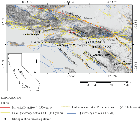
Shaded relief map of southern California showing Quaternary-active faults (lines) and the approximate locations (black circles) of the six strong-motion recording stations and our seismic surveys. Quaternary fault data was acquired from the U.S. Geological Survey Quaternary Fault and Fold Database of the United States (https://usgs.maps.arcgis.com/apps/webappviewer/index.html?id=5a6038b3a1684561a9b0aadf88412fcf, U.S. Geological Survey Earthquake Hazards Program, 2020).
Table 1.
Total number of traces used for P- and S-wave inversion to develop seismic velocity models (Hole, 1992).[Each column shows the number of traces generated by different seismic sources for each of the 7 profiles (Chan and others, 2021). kg, kilograms; °, degrees; AWD, accelerated weight-drop; NA, not applicable]
Profile LA17-1—Olinda (SCSN OLI)
Profile LA17-1-OLI was oriented west to east on an elevated dirt path, adjacent to the Southern California Edison (SCE) Olinda substation (fig. 2). The strong-motion recording station (SCSN OLI) was in the southwest corner of the substation, approximately 65 m from the nearest geophone of the seismic profile. We deployed 82 P- and S-wave geophones at 2-m intervals along the profile and co-located P-wave (226-kg vertical AWD) and S-wave (3.5-kg sledgehammer) sources. We also used a 45°-angle AWD S-wave source approximately every 20 m along the profile and a 2.7-kg hammer and steel plate P-wave source approximately every 24 m along the profile.
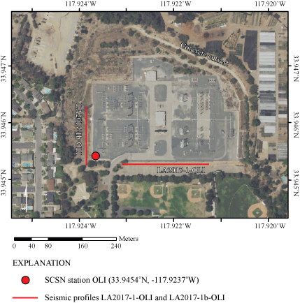
Orthoimage showing seismic profiles LA17-1-OLI and LA17-1b-OLI (red lines) adjacent to Southern California Edison substation in La Habra, Calif. Strong-motion recording station SCSN OLI is in the southwest corner of the substation (red circle). The concrete culvert visible in the upper right-hand corner of the image shows the water drainage rerouted away from the substation. (SCSN, Southern California seismic network). Orthoimage was acquired from The National Map-Orthoimagery (https://apps.nationalmap.gov/viewer/, U.S. Geological Survey National Geospatial Program, 2009).
Profile LA17-1b—Olinda (SCSN OLI)
Profile LA17-1b-OLI was oriented south to north, adjacent to the SCE Olinda substation (fig. 2). The strong-motion recording station (SCSN OLI) was approximately 15 m from the closest geophone of the seismic profile. We deployed 30 P-wave geophones at 4-m spacing along the profile and co-located P-wave (226-kg AWD) seismic sources. S-wave (body waves) data were not acquired along profile LA17-1b-OLI due to time limitations.
Profile LA17-2—Serrano (SCSN SRN)
Profile LA17-2-SRN was oriented southwest to northeast inside the SCE Serrano substation (fig. 3). The strong-motion recording station (SCSN SRN) was approximately 200 m southeast of the closest geophone of the seismic profile. We deployed 88 P- and S-wave wave geophones along the profile, with 2-m spacing between geophones. We co-located P-wave (226-kg AWD) and S-wave (3.5-kg sledgehammer) sources with the geophones (1-m offset), including a 45°-angle AWD S-wave source approximately every 20 m along the profile and a 2.7-kg hammer and steel plate P-wave source approximately every 36 m along the profile.
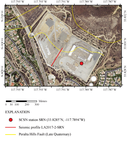
Orthoimage showing seismic profile LA17-2-SRN (red line) inside a Southern California Edison substation in Orange, Calif. Strong-motion recording station SCSN SRN is in the southeastern area of the substation (red circle). The late Quaternary Peralta Hills Fault (yellow lines) is mapped crossing the substation and our seismic profile (SCSN, Southern California seismic network). Orthoimage was acquired from The National Map-Orthoimagery (https://apps.nationalmap.gov/viewer/, U.S. Geological Survey National Geospatial Program, 2009).
Profile LA17-3—Murrieta (SCSN MUR)
Profile LA17-3-MUR was oriented southwest to northeast, adjacent to the SCE Murrieta substation (fig. 4). The strong-motion recording station (SCSN MUR) was located approximately 40 m southwest of the nearest geophone of the seismic profile. We deployed 60 P- and S-wave geophones at 2-m spacing along the profile and co-located P-wave (226-kg AWD) and S-wave (3.5-kg sledgehammer) sources. We also generated S-wave sources using the 45°-angle AWD source and a 2.7-kg hammer and steel plate P-wave source approximately every 20 m along the profile.
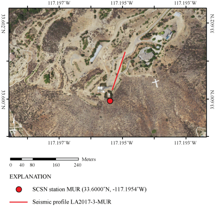
Orthoimage showing seismic profile LA17-3-MUR (red line) adjacent to Southern California Edison substation in Murrieta, Calif. Strong-motion recording station SCSN MUR is in the southeast area of the substation (red circle); (SCSN, Southern California seismic network). Orthoimage was acquired from The National Map-Orthoimagery (https://apps.nationalmap.gov/viewer/, U.S. Geological Survey National Geospatial Program, 2009).
Profile LA17-4—La Cienega (SCSN LCG)
Profile LA17-4-LCG was oriented southeast to northwest, adjacent to the SCE La Cienega substation (fig. 5). The strong-motion recording station (SCSN LCG) was approximately 130 m northwest of the closest geophone of the seismic profile. We deployed 60 P- and S-wave geophones at 2-m spacing along the profile, with co-located S-wave (3.5-kg sledgehammer) seismic sources. P-wave (226-kg AWD) sources were located at every other geophone (4 m spacing) along the profile. We did not use the 45°-angle AWD S-wave or the 2.7-kg hammer and steel plate P-wave sources along this profile due to time limitations.
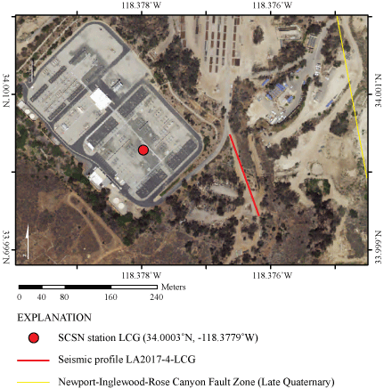
Orthoimage showing seismic profile LA17-4-LCG (red line) east of Southern California Edison substation in Ladera Heights, Calif. Strong-motion recording station SCSN LCG is in the eastern area of the substation (red circle). Late Quaternary Newport-Inglewood-Rose Canyon Fault Zone (yellow line) is mapped less than 200 meters northeast of our seismic profile. (SCSN, Southern California seismic network). Orthoimage was acquired from The National Map-Orthoimagery (https://apps.nationalmap.gov/viewer/, U.S. Geological Survey National Geospatial Program, 2009).
Profile LA17-5—Rush (SCSN RUS)
Profile LA17-5-RUS was oriented southeast to northwest, adjacent to the SCE Rush substation (fig. 6). The strong-motion recording station (SCSN RUS) was approximately 90 m southwest of the nearest geophone of the seismic profile. We deployed 60 P- and S-wave geophones at 2-m spacing along the profile and co-located P-wave (226-kg AWD) and S-wave (3.5-kg sledgehammer) sources. We did not use the 45°-angle AWD S-wave or the 2.7-kg hammer and steel plate P-wave sources here due to time limitations.
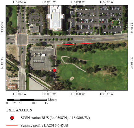
Orthoimage showing seismic profile LA17-5-RUS (red line) northeast of a Southern California Edison substation in Rosemead, Calif. Strong-motion recording station SCSN RUS is in the southeast corner of the substation (red circle); (SCSN, Southern California seismic network). Orthoimage was acquired from The National Map-Orthoimagery (https://apps.nationalmap.gov/viewer/, U.S. Geological Survey National Geospatial Program, 2009).
Profile LA17-6—Santa Clara (SCSN STC)
Profile LA17-6-STC was oriented southeast to northwest, adjacent to the SCE Santa Clara substation (fig. 7). The strong-motion recording station (SCSN STC) was in the northwest corner of the substation, approximately 250 m northwest of the seismic profile. We deployed 60 P- and S-wave geophones at 2-m spacing along the profile and co-located P-wave (226-kg AWD) and S-wave (3.5-kg sledgehammer) sources. We did not use the 45°-angle AWD S-wave or the 2.7-kg hammer and steel plate P-wave sources at this site due to time limitations.
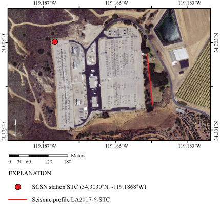
Orthoimage showing seismic profile LA17-6-STC (red line) east of Southern California Edison substation in Ventura, Calif. Strong-motion recording station SCSN STC is in northwest corner of the substation (red circle); (SCSN, Southern California seismic network). Orthoimage was acquired from The National Map-Orthoimagery (https://apps.nationalmap.gov/viewer/, U.S. Geological Survey National Geospatial Program, 2009).
Seismic-Imaging Methods
We used an acquisition geometry that allowed us to develop 2-D P- and S-wave refraction tomography models, tomographic-based VP/VS and Poisson’s ratio models (all based on body waves), and VS models based on Rayleigh and Love waves using the multichannel analysis of surface waves (MASW) method.
Refraction-Tomography Modeling
We used refraction tomography to model subsurface P- and S-wave velocities along all profiles. We first processed the seismic data (Chan and others, 2021) by grouping the recorded seismic traces into shot gathers and adding the survey geometry. We removed traces without recorded signals and corrected the timing of each shot gather to match the timing of each P- and S-wave source. First arrivals from P- and S-wave shot gathers were inverted (table 1) to develop seismic-velocity models using the algorithm of Hole (1992). We developed P- and S-wave starting models based on one-dimensional (1-D) modeling of the shot gathers, and we parameterized our initial 2-D models into vertical and horizontal grids with each grid space at 2-m based on shot and geophone spacing. The total number of traces ranged between 420 and 7,743 for each seismic profile (table 1), and, generally, the large number of first arrivals used for each profile allows for a well-determined velocity model.
Multichannel Analysis of Surface Waves (MASW)
Our data-acquisition method allows us to use Rayleigh- and Love-waves to develop 2-D S-wave velocity models from vertical- and horizontal-component data, respectively, using the MASW method. The MASW method utilizes the dispersive nature of surface waves to estimate VS velocities in the shallow subsurface (Park and others, 1999; Xia and others, 1999). The MASW technique is often used on surface waves in geotechnical site investigations and shallow subsurface studies (Pujol, 2003; Ivanov and others, 2003, 2008, 2013; Miller and others, 1999; Park and others, 1999, 2007; Zeng and others, 2012; Park, 2013; Xia and others, 2000; Yong and others, 2013). We used the common midpoint cross-correlation (CMPCC) method, developed by Hayashi and Hikima (2003) and Hayashi and Suzuki (2004), to construct phase velocity (dispersion) curves from all receivers along each profile. In our analysis, we grouped cross-correlated pairs of seismic traces with common midpoints and converted the CMPCC gathers from time-distance waveform data to images of phase velocity-frequency through an integral transformation. We examined and manually adjusted the fundamental mode dispersion curve picks before inverting the selected picks using a non-linear, least-squares approach. Our starting models (table 2) extended to between 40 and 50 m depth, consisted of 15 layers, and were inverted using up to 10 iterations. The starting model depths were based on one-half to one-third of the length of each seismic profile, whereas other parameters were based on starting models from prior studies with similar underlying geology and topography. Finally, the multiple 1-D VS models along each profile were combined to make 2-D VS models.
VS30 Calculations
We evaluated the time-averaged VS in the upper 30 m of the subsurface (VS30) from (a) our tomographic Vs models, (b) our MASW Rayleigh-wave models (MASRW), and (c) our MASW Love-wave models (MASLW). VS30 is frequently used to evaluate soil properties (Holtzer and others, 2005) and to account for site amplification in ground-motion models (Baltay and Boatwright, 2015) and in ground-motion prediction equations (GMPEs). VS30 is also used to determine site classification, which is an important consideration for establishing building codes for seismic safety (Building Seismic Safety Council, 2003). We calculated VS30 at every 1 m along all profiles for areas of our models with VS values to at least 30 m depth. For parts of our model where VS was not measured to depths of at least 30 m, we calculated VSZ (VS as a function of depth) using interpolated shear-wave velocities to 30 m depth. From our models, we evaluated lateral variations in VS30 across the seismic profiles, and we compared VS30 that were calculated using the multiple modeling methods (Catchings and others, 2017; 2019, Chan and others, 2018a; 2018b).
Velocity Models and Dispersion Curves
In the following sections, we present the various velocity models that we developed using the techniques described above. Appendix 1 shows Rayleigh- and Love-wave dispersion curves nearest to the strong-motion recording stations along each seismic profile. Appendix 2 shows Rayleigh- and Love-wave dispersion curve picks along the entire lengths of the profiles. Appendix 3 shows 1-D velocity-depth profiles nearest to the strong-motion recording stations along each seismic profile. We did not analyze seismic data generated by the 2.7-kg hammer because the source provided no additional seismic information to the refraction tomography and MASW methods.
Profile LA17-1—Olinda (SCSN OLI)
P-wave Refraction Tomography (VP) Model
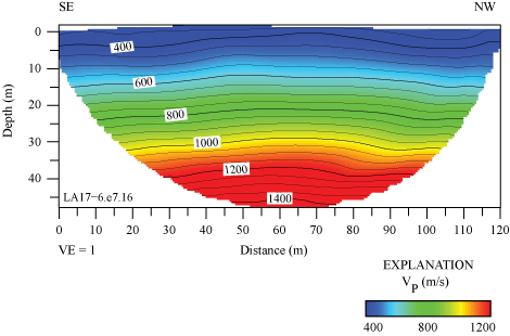
Along the Olinda LA17-1-OLI seismic profile, P-wave velocities (VP) range from approximately 375 meters per second (m/s) near the surface to approximately 1,050 m/s at 40 m depth (fig. 8). Below about 5 m depth, velocity contours and gradients are generally sub-parallel to the surface, and there are slightly higher velocities in the western part of the seismic profile. The strong-motion recording station (SCSN OLI) was located approximately 65 m west of our seismic profile and was nearest to distance meter 0.
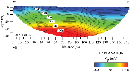
P-wave refraction tomography model for profile LA17-1-OLI. P-wave velocities range from approximately 375 meters per second (m/s) in the near surface to 1,050 m/s at 40 m depth. P-wave velocities are higher near the west end of the seismic profile and at depth. (W, west; E, east; VE, vertical exaggeration; VP, P-wave velocity.)
S-wave Refraction Tomography (VS) Model
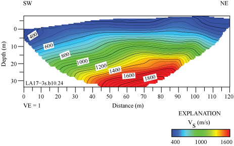
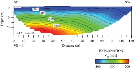
Determined from refraction tomography, VS values range from approximately 200 near the surface to approximately 1,100 m/s at 60 m depth (fig. 9). Similar to the P-wave refraction model, VS gradients are generally sub-parallel to the surface in the western part of the profile, with slightly higher velocities in the upper 20 m of the subsurface to the west. We calculated the range of VS30 across the profile to range from 290 to 362 m/s, with a VS30 of 320 m/s nearest to the strong-motion recording station (SCSN OLI) at distance meter 0 (table 3). To determine VS30 at meter 0, velocities near the center of the profile at 30 m depth are assumed to extend horizontally to meter 0.
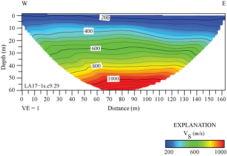
S-wave refraction tomography model for profile LA17-1-OLI. S-wave velocities range from approximately 200 meters per second (m/s) near the surface to approximately 1100 m/s at 60 meters (m) depth. S-wave velocities are slightly higher near the western half of the seismic profile. (W, west; E, east; VE, vertical exaggeration; VS, S-wave velocity.)
Table 3.
VS30 values for seven seismic profiles near strong-motion recording stations located at Southern California Edison substations.[m/s, meters per second; NA, not applicable; 2-D, two dimensional; kg, kilograms; AWD, accelerated weight-drop]
MASRW 2-D S-wave Velocity Model
A Rayleigh-wave dispersion curve shown in appendix 1 (fig. 1.1A) was developed for the location (meter 0) along our seismic profile nearest to the SCSN OLI strong-motion recording station. Fundamental mode dispersion curve picks (red circles) are between phase velocities of approximately 250 and 2,300 m/s and frequencies between 2 and 17 Hz. Rayleigh-wave fundamental mode dispersion curve picks across the entire length of the profile (fig. 2.1A) generally coincide with phase velocities between approximately 200 and 2,500 m/s and frequencies between 3 and 20 Hz. The Rayleigh-wave 1-D depth-velocity model (fig. 3.1A) nearest to the strong-motion recording station shows a weak positive gradient in VS in the upper 30 m of the subsurface and stronger positive gradient in Vs below 30 m depth. We calculated (a) VS30 to be 371 nearest to the SCSN OLI strong-motion recording station, with (b) VS30 ranging from 237 to 371 m/s, and (c) an average VS30 of 291 m/s across the profile (table 3).
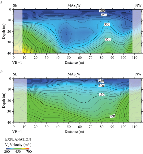
We developed a VS model for the LA17-1-OLI seismic profile by evaluating Rayleigh-waves with the MASW technique. Our 2-D VS model (fig. 10A) shows VS ranges from approximately 150 m/s near the surface to 650 m/s at 40 m depth. VS is slightly higher at depth in the western half of the seismic profile, with channel-like velocity structure at depth near distance meter 130.
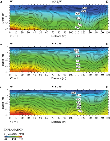
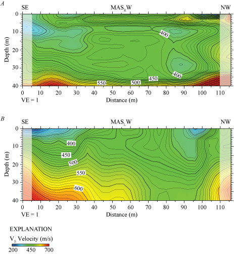
Two-dimensional MASRW and MASLW shear-wave velocity models for profile LA17-1-OLI. A, S-wave velocities for our MASRW model range from approximately 150 meters per second (m/s) near the surface to approximately 650 m/s at 40 meters (m) depth. B, MASLW model developed from data generated by a 3.5-kilogram-sledgehammer and aluminum shear-wave block source. S-wave velocities range from approximately 150 m/s near the surface to approximately 650 m/s at 40 m depth. C, MASLW model developed from data generated by a 45°-angle accelerated weight-drop and aluminum shear-wave block source. S-wave velocities range from approximately 150 m/s near the surface to approximately 650 m/s at 40 m depth. All three multichannel analysis of surface waves models show slightly higher S-wave velocities in the western third of the seismic profile and a channel-like velocity structure near distance meter 130. (W, west; E, east; VE, vertical exaggeration; VS, S-wave velocity.)
MASLW 2-D S-wave Velocity Model—3.5-kg Sledgehammer Source
The Love-wave dispersion curve shown in appendix 1 (fig. 1.1B) was developed for the location along our seismic profile nearest to the SCSN OLI strong-motion recording station (meter 0). Fundamental mode dispersion curve picks (red circles) are between phase velocities of approximately 250 and 2,300 m/s and frequencies between 2 and 26 Hz; we do not observe higher mode dispersion curves. The Love-wave fundamental mode dispersion curve picks across the entire length of the profile (fig. 2.1B) generally coincide with phase velocities between approximately 200 and 2,500 m/s at frequencies between 2 and 25 Hz. The Love-wave 1-D depth-velocity profile (fig. 3.1B) nearest to the strong-motion recording station shows a gradual increase in VS below approximately 10 m depth. We calculated (a) VS30 to be 494 m/s nearest to the SCSN OLI strong-motion recording station, with (b) VS30 ranging from 241 to 494 m/s, as calculated for each meter along the profile. The average VS30 across the entire profile is 289 m/s. (table 3).
Our 2-D MASLW VS model along the LA17-1-OLI seismic profile (fig. 10B) indicates VS ranges from approximately 150 m/s near the surface to approximately 650 m/s at 40 m depth. Modeled velocities are slightly higher at depth in the western half of the seismic profile, with a channel-like velocity structure near distance meter 130.
MASLW 2-D S-wave Velocity Model—45°-Angle Weight-Drop Source
A Love-wave dispersion curve shown in appendix 1 (fig. 1.1C) was developed for the location (meter 0) along our seismic profile that was nearest to the SCSN OLI strong-motion recording station. Fundamental mode dispersion curve picks (red circles) coincide with phase velocities between approximately 250 and 2,300 m/s at frequencies between 2 and 24 Hz; we do not observe higher mode dispersion curves. The Love-wave fundamental mode dispersion curve picks across the entire length of the profile (fig. 2.1C) generally coincide with phase velocities between approximately 200 and 2,000 m/s at frequencies between 2 and 25 Hz. The Love-wave 1-D velocity-depth model (fig. 3.1C) nearest to the strong-motion recording station shows gradual positive gradient in VS below approximately 10 m depth. We calculated (a) VS30 to be 410 m/s nearest to the SCSN OLI strong-motion recording station, with (b) VS30 ranging from 258 to 410 m/s (as measured at each meter along the profile), and (c) an average VS30 of 309 m/s along the entire profile (table 3).
Our 2-D MASLW VS model along the LA17-1-OLI seismic profile (fig. 10C) shows that VS ranges from approximately 150 m/s near the surface to approximately 650 m/s at 40 m depth. Modeled VS is slightly higher at depth in the western half of the seismic profile, with a channel-like velocity structure near distance meter 130.
Profile LA17-1b—Olinda (SCSN OLI)
P-wave Refraction Tomography (VP) Model
VP ranges from approximately 500 m/s near the surface to approximately 1,800 m/s at 45 m depth (fig. 11). Velocity contours are generally sub-parallel, and there are slightly higher velocities in the southern half of the seismic profile. The strong-motion recording station (SCSN OLI) is approximately 10 m east of our seismic profile and nearest to distance meter 16. The 1,500 m/s contour, which has been shown to coincide with the top of groundwater in other studies (Catchings and others, 2001, 2006, 2013, 2014, 2017), is located at approximately 30–40 m depth.
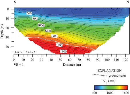
P-wave refraction tomography model for profile LA17-1b-OLI. P-wave velocities range from approximately 500 meters per second (m/s) near the surface to approximately 1,800 m/s at approximately 45 meters (m) depth. P-wave velocities are higher near the south end of the seismic profile at depth. Prior studies suggest the top of groundwater (white dashed line) coincides with 1,500 m/s P-wave velocity contour. (S, south; N, north; VE, vertical exaggeration; VP, P-wave velocity.)
MASRW 2-D S-wave Velocity Model
An MASRW Rayleigh-wave dispersion curve shown in appendix 1 (fig. 1.1D) was developed for the location (meter 16) along our seismic profile that was nearest to the SCSN OLI strong-motion recording station. Fundamental mode dispersion curve picks (red circles) coincide with phase velocities between approximately 250 and 1,400 m/s and frequencies between 3 and 12 Hz. Rayleigh-wave fundamental mode dispersion curve picks across the entire length of the profile (fig. 2.1D) generally coincide with phase velocities between approximately 200 and 1,500 m/s at frequencies between 3 and 21 Hz. The Rayleigh-wave 1-D velocity-depth model (fig. 3.1D) for the geophone nearest to the strong-motion recording station shows a gradual positive gradient in VS below approximately 8 m depth. We calculated (a) VS30 to be 336 m/s nearest to the SCSN OLI strong-motion recording station, with (b) a range of VS30 between 281 and 362 m/s (measured at each meter along the profile), and (c) an average VS30 of 309 m/s for the entire profile (table 3).
Our 2-D MASRW VS model along the LA17-1b-OLI seismic profile (fig. 12) indicates that VS ranges from approximately 200 m/s near the surface to approximately 550 m/s at 40 m depth. Model velocity contours are generally sub-parallel, and VS is slightly higher at depth in the southern third (between distance meters 0 and 40) of the seismic profile. We observe high-velocity contours in the upper south corner of the model, which we interpret as artifacts due to lack of S-wave data in that area.
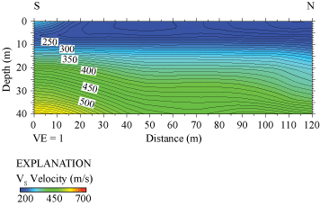
Two-dimensional MASRW shear-wave velocity model for profile LA17-1b-OLI. S-wave velocities for our MASRW model range from approximately 200 meters per second (m/s) near the surface to approximately 550 m/s at 40 meters (m) depth. (S, south; N, north; VE, vertical exaggeration; VS, S-wave velocity.)
Profile LA17-2—Serrano (SCSN SRN)
P-wave Refraction Tomography (VP) Model
VP ranges between approximately 700 m/s near the surface to approximately 2,000 m/s at 50 m depth (fig. 13). VP is lower near both the southwest and northeast ends of the seismic profile. The SCSN SRN strong-motion recording station was approximately 200 m southeast of our seismic profile and nearest to distance meter 124. The 1,500 m/s velocity contour (top of groundwater) varies between about 35 and 45 m beneath the surface.
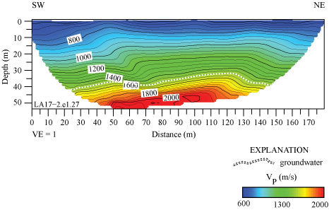
P-wave refraction tomography model for profile LA17-2-SRN. P-wave velocities range from approximately 700 meters per second (m/s) near the surface to approximately 2,000 m/s at approximately 45 meters (m) depth. Top of groundwater is shown as a dashed line. (SW, southwest; NE, northeast; VE, vertical exaggeration; VP, P-wave velocity.)
S-wave Refraction Tomography (VS) Model
VS determined from refraction tomography ranges from approximately 400 m/s near the surface to approximately 900 m/s at 40 m depth (fig. 14). VS is lower near the northeast end of the seismic profile between distance meters 100 and 170. We calculated (a) VS30 along the profile to range between 470 and 588 m/s (measured at each meter along the profile), with (b) a VS30 of 537 m/s nearest (meter 124) to the SCSN SRN strong-motion recording station (table 3).
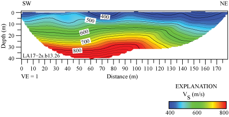
S-wave refraction tomography model for profile LA17-2-SRN. S-wave velocities range from approximately 400 meters per second (m/s) near the surface to approximately 900 m/s at approximately 40 meters (m) depth. S-wave velocities are lower near the northeast end of the seismic profile. (SW, southwest; NE, northeast; VE, vertical exaggeration; VS, S-wave velocity.)
MASRW 2-D S-wave Velocity Model
We present an MASRW (Rayleigh-wave) dispersion curve (fig. 1.2A) for the location (meter 124) along our seismic profile nearest to the SCSN SRN strong-motion recording station. Fundamental mode dispersion curve picks (red circles) coincide with phase velocities between approximately 250 and 1,000 m/s at frequencies between 4 and 22 Hz. Rayleigh-wave fundamental mode dispersion curve picks along the entire length of the profile (fig. 2.2A) generally coincide with phase velocities between approximately 250 and 2,500 m/s at frequencies between 2 and 40 Hz. Our Rayleigh-wave 1-D depth-velocity profile (fig. 3.2A) at the geophone nearest to the strong-motion recording station shows a positive gradient in VS below approximately 2 m depth. We calculated (a) VS30 to be 379 m/s nearest to the SCSN SRN strong-motion recording station, with (b) VS30 ranging between 344 and 429 m/s (measured at each meter along the profile), and (c) an average VS30 of 383 m/s along the entire profile (table 3).
We developed a VS model for the LA17-2-SRN seismic profile by evaluating Rayleigh-waves with the MASW technique. Our 2-D MASRW VS model for the LA17-2-SRN seismic profile (fig. 15A) indicates VS ranges from approximately 300 m/s near the surface to approximately 900 m/s at 50 m depth. Our model shows undulating velocity contours below approximately 20 m depth along the entire seismic profile.
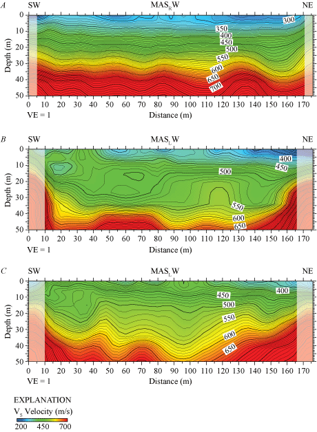
Two-dimensional MASRW and MASLW shear-wave velocity models for profile LA17-2-SRN. A, S-wave velocities for our MASRW model range from approximately 300 meters per second (m/s) near the surface to approximately 900 m/s at 50 meters (m) depth. B, MASLW model developed from data generated by 3.5-kilogram sledgehammer and aluminum shear-wave block sources. S-wave velocities range from approximately 350 m/s near the surface to approximately 850 m/s at 50 m depth. C, MASLW model developed from data generated by 45°-angle accelerated weight-drop and aluminum shear-wave block sources. S-wave velocities range from approximately 350 m/s near the surface to 800 m/s at 50 m depth. All three multichannel analysis of surface waves models show undulating velocity contours along the entire profile. Shaded areas represent regions with few data points. (SW, southwest; NE, northeast; VE, vertical exaggeration; VS, S-wave velocity.)
MASLW 2-D S-wave Velocity Model—3.5-kg Sledgehammer Source
The MASLW (Love-wave) dispersion curve shown in figure 1.2B was developed for the location (meter 124) along our seismic profile nearest to the SCSN SRN strong-motion recording station. Fundamental mode dispersion curve picks (red circles) coincide with phase velocities between approximately 250 and 1,200 m/s at frequencies between 2 and 30 Hz. The Love-wave fundamental mode dispersion curve picks along the entire length of the profile (fig. 2.2B) generally coincide with phase velocities between approximately 250 and 2,500 m/s at frequencies between 1 and 40 Hz. Our Love-wave 1-D velocity depth model (fig. 3.2B) for the location nearest to the strong-motion recording station shows a gradual increase in VS between approximately 2 and 20 m depth, then a gradual decrease in VS between approximately 20 and 40 m depth. We calculated (a) VS30 to be 432 m/s nearest to the SCSN SRN strong-motion recording station, with (b) the VS30 ranging from approximately 415 to approximately 475 m/s (measured at each meter along the profile), and (c) VS30 averaging 444 m/s along the entire profile (table 3).
Our 2-D MASLW VS model along the LA17-2-SRN seismic profile (fig. 15B) shows VS ranges from approximately 350 m/s near the surface to approximately 850 m/s at 50 m depth. Our model shows undulating velocity contours, which suggest complex geologic structures, such as bedrock, at depth.
MASLW 2-D S-wave Velocity Model—45°-Angle Weight-Drop Source
An MASLW (Love-wave) dispersion curve shown in figure 1.2C was developed for the location (meter 124) of our seismic profile that was nearest to the SCSN SRN strong-motion recording station. Fundamental mode dispersion curve picks (red circles) are between phase velocities approximately 250 and 1,100 m/s at frequencies between 2 and 30 Hz. Love-wave fundamental mode dispersion curve picks across the entire length of the profile (fig. 2.2C) are generally at phase velocities between approximately 250 and 1,600 m/s at frequencies between 2 and 40 Hz. Our Love-wave 1-D velocity-depth model (fig. 3.2C) for the location nearest to the strong-motion recording station shows a gradual increase in VS below approximately 2 m depth. We calculated (a) VS30 to be 443 m/s nearest to the SCSN SRN strong-motion recording station, with (b) VS30 ranging between 435 and 486 m/s (measured at each meter along the profile) and (c) VS30 averaging 462 m/s along the profile (table 3).
Our 2-D MASLW VS model along the seismic profile LA17-2-SRN (fig. 15C) indicates VS ranges between approximately 350 m/s at the near surface to 800 m/s at 50 m depth. Our model shows undulating velocity contours, which suggest complex structures at depth.
Profile LA17-3—Murrieta (SCSN MUR)
P-wave Refraction Tomography (VP) Model
Along the SCSN MUR seismic profile, VP ranges between approximately 500 m/s near the surface and approximately 3,500 m/s at 30 m depth (fig. 16). VP is lower near the southwest end of the seismic profile, between distance meters 0 and 70. The SCSN MUR strong-motion recording station is approximately 40 m southwest of our seismic profile and nearest to distance meter 0. The 1,500 m/s velocity contour (top of groundwater) varies between about 10 and 25 m beneath the surface, and the top of groundwater appears shallower in the northeastern half of the profile (distance meter 50 to 120).
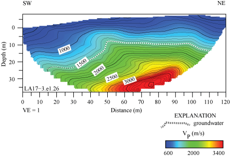
P-wave refraction tomography model for profile LA17-3-MUR (station SCSN MUR). P-wave velocities range between approximately 500 meters per second (m/s) near the surface and 3,500 m/s at approximately 30 meters (m) depth. Top of groundwater is shown as a dashed line. (SW, southwest; NE, northeast; VE, vertical exaggeration; VP, P-wave velocity.)
S-wave Refraction Tomography (VS) Model
VS along the SCSN MUR seismic profile, as determined from refraction tomography, ranges between approximately 400 m/s near the surface and approximately 1,800 m/s at 30 m depth (fig. 17). Similar to the VP model, VS is lower near the southwest end of the seismic profile between distance meters 0 and 70. On the basis of our VS tomography model, we calculated VS30 along the profile, which ranges between 497 and 769 m/s (measured at each meter along the profile), and the VS30 nearest to the SCSN MUR strong-motion station (distance meter 0) is 497 m/s (table 3).
S-wave refraction tomography model for profile LA17-3-MUR (SCSN MUR). S-wave velocities range between approximately 400 meters per second (m/s) near the surface and 1,800 m/s at approximately 30 meters (m) depth. VS is lower along the southwestern half of the seismic profile. (SW, southwest; NE, northeast; VE, vertical exaggeration; VS, S-wave velocity.)
MASRW 2-D S-wave Velocity Model
We present a Rayleigh-wave dispersion curve (fig. 1.3A) for the location (meter 0 of our seismic profile) nearest to the SCSN MUR strong-motion recording station. Fundamental mode dispersion curve picks (red circles) range between phase velocities of approximately 250 and 1,500 m/s at frequencies between 4 and 20 Hz. Rayleigh-wave fundamental mode dispersion curve picks along the length of the profile (fig. 2.3A) range between phase velocities of approximately 100 and 2,600 m/s at frequencies between 4 and 45 Hz. Our derived Rayleigh-wave 1-D velocity model (fig. 3.3A) for the area of the SCSN MUR seismic profile nearest to the strong-motion recording station includes a positive gradient between approximately 8 and approximately 18 m depth and below approximately 36 m depth. From the Rayleigh-wave data, we calculated (a) VS30 to be 613 m/s nearest to the SCSN MUR strong-motion recording station, with (b) a range of VS30 between 557 and 651 m/s along the profile (calculated at each meter along the profile), and (c) an average VS30 of 592 m/s for the entire profile (table 3).
We developed a VS model for the LA17-3-MUR seismic profile by evaluating Rayleigh-waves with the MASW technique. Our 2-D MASRW VS model for the SCSN MUR seismic profile (fig. 18A) suggests VS ranges between approximately 300 m/s near the surface and approximately 1400 m/s at 40 m depth. Our model shows undulating velocity contours below approximately 8 m depth and channel-like structures centered near distance meters 40 and 80 along the profile. VS is higher near the northeast end of the profile below approximately 5 m depth.
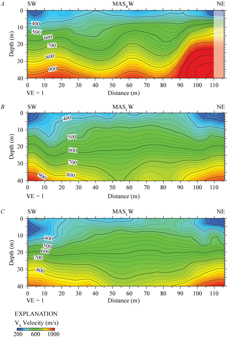
Two-dimensional MASRW and MASLW VS models for profile LA17-3-MUR near the SCSN MUR strong-motion recording station. A, VS for MASRW model ranges between approximately 300 meters per second (m/s) near the surface and approximately 1,400 m/s at 40 meters (m) depth. Gray box between distance meters 110 and 115 represents an area of low confidence due to unclear dispersion curves. B, MASLW VS model derived from data generated by the 3.5-kilogram sledgehammer and aluminum block source. VS ranges between approximately 300 m/s near the surface and 900 m/s at 40 m depth. C, MASLW VS model derived from data generated by the 45°-angle accelerated weight-drop and aluminum block source. VS ranges between approximately 300 m/s near the surface and 900 m/s at 40 m depth. All three multichannel analysis of surface waves models show undulating velocity contours across the profile. (SW, southwest; NE, northeast; VE, vertical exaggeration; VS, S-wave velocity.)
MASLW 2-D S-wave Velocity Model—3.5-kg Sledgehammer Source
We present a Love-wave dispersion curve (fig. 1.3B) for the location (meter 0 of our seismic profile) nearest to the SCSN MUR strong-motion recording station. Fundamental mode dispersion curve picks (red circles) range between phase velocities approximately 250 and 1,500 m/s and frequencies between 4 and 32 Hz. Love-wave fundamental mode dispersion curve picks for sites along the length of the profile (fig. 2.3B) generally coincide with phase velocities between approximately 200 and 1,500 m/s and frequencies between 3 and 33 Hz. Our Love-wave 1-D velocity model (fig. 3.3B) for the site (meter 0) nearest to the strong-motion recording station indicates a positive VS gradient at all depths. From the Love-wave data, we calculated (a) VS30 to be 318 m/s nearest to the SCSN MUR strong-motion recording station, with (b) a range of VS30 between 318 and 508 m/s (calculated at every meter along the profile), and (c) an average VS30 of 463 m/s for the entire profile (table 3).
We developed a 2-D MASLW VS model for the seismic profile LA17-3-MUR (fig. 18B) near the SCSN MUR strong-motion station. Our model indicates VS ranges between approximately 300 m/s near the surface and approximately 900 m/s at 40 m depth. Our model shows undulating velocity contours along much of the profile, with VS values higher below approximately 25 m near the northeast and southwest ends of the profile.
MASLW 2-D S-wave Velocity Model—45°-Angle Weight-Drop Source
We present a Love-wave dispersion curve (fig. 1.3C) for the location (meter 0) on our seismic profile nearest to the SCSN MUR strong-motion recording station. Fundamental mode dispersion curve picks (red circles) range between phase velocities of approximately 250 and 1,500 m/s and frequencies between 4 and 32 Hz. Love-wave fundamental mode dispersion curve picks across the length of the profile (fig. 2.3C) are generally at phase velocities between approximately 200 and 2,500 m/s and frequencies between 3 and 30 Hz. The Love-wave 1-D depth-velocity profile (fig. 3.3C) nearest to the strong-motion recording station shows a gradual increase in VS at all depths. We calculated (a) VS30 to be 318 m/s nearest to the SCSN MUR strong-motion recording station, (b) VS30 at each meter along the profile to range between 318 and 543 m/s, and (c) the average VS30 along the entire profile to be 491 m/s (table 3).
Our 2-D MASLW VS model along the LA17-3-MUR seismic profile (fig. 18C) shows VS ranges between approximately 300 m/s near the surface and approximately 900 m/s at 40 m depth. Our model shows undulating velocity contours throughout much of the profile, and VS is higher below approximately 25 m at both the northeast and southwest ends of the profile.
Profile LA17-4—La Cienega (SCSN LCG)
P-wave Refraction Tomography (VP) Model
Along the LA17-4-LCG seismic profile near the SCSN LCG, VP ranges between approximately 700 m/s near the surface and approximately 2,200 m/s at 25 m depth (fig. 19). VP is relatively higher below approximately 10 m depth at distance meters between approximately 25 and 55. The SCSN LCG strong-motion recording station is approximately 120 m northwest of our seismic profile and nearest to distance meter 120 of the profile. The 1,500 m/s velocity contour (top of groundwater) varies between about 10 to 20 m beneath the surface.
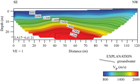
P-wave refraction tomography model for profile LA17-4-LCG. P-wave velocities (VP) range between approximately 700 m/s near the surface and 2,200 m/s at approximately 25 m depth. VP is lower in the northwest and southeast ends of the seismic profile. Top of groundwater is shown as a dashed line. (SE, southeast; NW, northwest; VE, vertical exaggeration; VP, P-wave velocity.)
S-wave Refraction Tomography (VS) Model
Our VS refraction tomography model along the LA17-4-LCG seismic profile indicates that VS ranges between approximately 400 m/s near the surface and approximately 1,100 m/s at 30 m depth (fig. 20). VS is relatively higher between distance meters approximately 20 and 60, with undulating velocity contours in the upper approximately 10 m of the subsurface. We calculated VS30 along the profile to be between 518 and 774 m/s. Calculated VS30 nearest to the SCSN LCG strong-motion station (at distance meter 120 of our seismic profile) is 595 m/s (table 3).
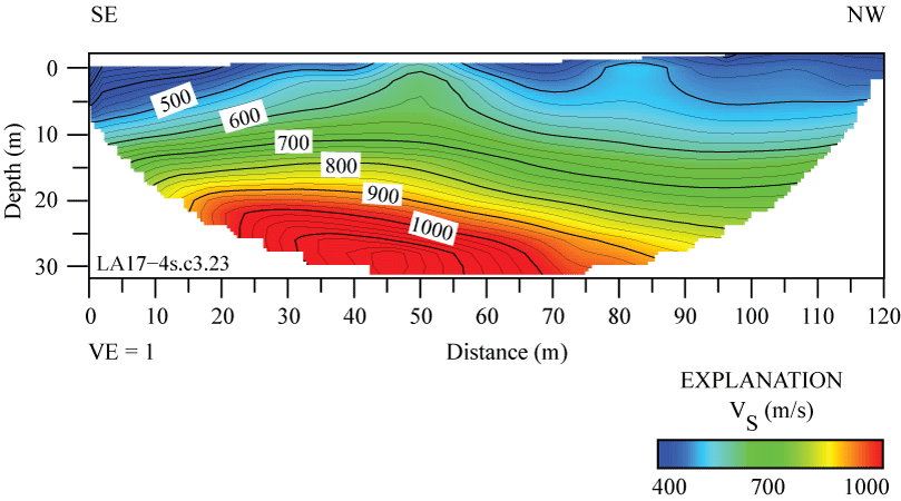
S-wave refraction tomography velocity model for profile LA17-4-LCG. VS ranges between approximately 400 meters per second (m/s) in the near surface and 1,100 m/s at approximately 30 meters (m) depth. VS is lower near the northwest and southeast ends of the seismic profile. (SE, southeast; NW, northwest; VE, vertical exaggeration; VS, S-wave velocity.)
MASRW 2-D S-wave Velocity Model
We present a Rayleigh-wave dispersion curve (fig. 1.4A) for the location (meter 120) on our seismic profile that is nearest to the SCSN LCG strong-motion recording station. Fundamental mode dispersion curve picks (red circles) are between phase velocities of approximately 250 and 1,600 m/s and frequencies between 2 and 56 Hz. Rayleigh-wave fundamental mode dispersion curve picks for the entire length of the profile (fig. 2.4A) are generally at phase velocities between approximately 250 and 1,500 m/s and frequencies between 2 and 56 Hz. Our Rayleigh-wave 1-D depth-velocity profile (fig. 3.4A) for our geophone that was nearest to the SCSN LCG strong-motion recording station shows a gradual increase in VS below approximately 12 m depth. We calculated (a) VS30 to be 425 m/s nearest to the SCSN LCG strong-motion recording station, (b) VS30 at each meter along the profile to range between 357 and 425 m/s, and (c) the average VS30 across the entire profile to be 374 m/s (table 3).
We developed a VS model for the LA17-4-LCG seismic profile by evaluating Rayleigh-waves with the MASW technique. Our 2-D MASRW VS model along the LA17-4-LCG seismic profile (fig. 21A) shows VS ranges between approximately 300 m/s near the surface and approximately 650 m/s at 40 m depth. Our model shows a channel-like structure (VS less than 400 m/s) centered at distance meter 90, extending to approximately 35 m depth. VS is generally between approximately 300 and 400 m/s in the upper 35 m of the subsurface and increases to approximately 650 m/s at depths between 35 and 40 m. VS is higher at the southeast end of the profile at depths below approximately 20 m.
Two-dimensional MASRW- and MASLW-derived shear-wave velocity models for profile LA17-4-LCG. A, MASRW-based VS ranges between approximately 300 meters per second (m/s) near the surface and approximately 650 m/s at approximately 40 meters (m) depth. B, MASLW data were generated using a 3.5-kilogram sledgehammer and aluminum block. VS ranges between approximately 300 m/s near the surface and 650 m/s at 40 m depth. Both MASW-based models show undulating and complex velocity contours along the entire profile. Shaded areas represent regions with few data points. (SE, southeast; NW, northwest; VE, vertical exaggeration; VS, S-wave velocity.)
MASLW 2-D S-wave Velocity Model—3.5-kg Sledgehammer Source
We show a Love-wave dispersion curve (fig. 1.4B) for the location (meter 120) along our seismic profile that was nearest to the SCSN LCG strong-motion recording station. Fundamental mode dispersion curve picks (red circles) correlate phase velocities between approximately 250 and 1,600 m/s and frequencies between 2 and 56 Hz. Love-wave fundamental mode dispersion curve picks along the entire length of the profile (fig. 2.4B) generally coincide with phase velocities between approximately 150 and 1,600 m/s and frequencies between 2 and 70 Hz. A Love-wave 1-D depth-velocity profile (fig. 3.4B) for the part of seismic profile nearest to the SCSN LCG strong-motion recording station shows a gradual increase in VS between 2 and 40 m depth. We calculated (a) VS30 to be 645 m/s nearest to the SCSN LCG strong-motion recording station, (b) VS30 at each meter along the profile to be between 513 and 645 m/s, and (c) the average VS30 along the entire profile to be 555 m/s (table 3).
We developed a 2-D MASLW VS model along the LA17-4-LCG seismic profile (fig. 21B) using Love-waves. Our model shows VS ranges between approximately 300 m/s near the surface and approximately 650 m/s at 40 m depth. Our model shows undulating velocity contours throughout much of the profile and a channel-like velocity structure (VS less than 500 m/s) centered at distance meter 90, which extends past the maximum depth of our model at 40 m. VS is relatively high below approximately 20 m near both the southeast and northwest ends of the profile.
Profile LA17-5—Rush (SCSN RUS)
P-wave Refraction Tomography (VP) Model
We developed a VP model along the LA17-5-RUS seismic profile near the SCSN RUS strong-motion recording station. Along our profile, VP ranges between approximately 300 m/s near the surface and approximately 1,700 m/s at 20 m depth (fig. 22). Velocity contours are generally sub-horizontal in the upper approximately 13 m of the subsurface, and VP is generally higher between distance meters 0 and 50 along the profile. The SCSN RUS strong-motion recording station is approximately 87 m southwest of our seismic profile and nearest to distance meter 0 of the profile. The 1,500 m/s velocity contour (top of groundwater) appears at two discreet locations at depths below approximately 15, which may suggest a perched water table.
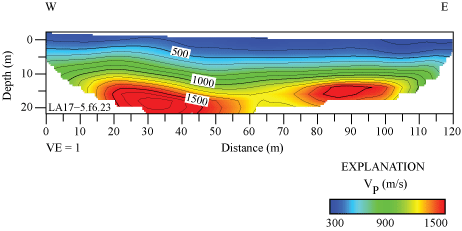
P-wave refraction tomography velocity model for the LA17-5-RUS profile. VP ranges between approximately 300 meters per second (m/s) near the surface and 1,700 m/s at approximately 20 meters (m) depth. VP is relatively higher near the western half of the profile at all depths. (W, west; E, east; VE, vertical exaggeration; VP, P-wave velocity.)
S-wave Refraction Tomography (VS) Model
We developed a S-wave refraction tomography model along the LA17-5-RUS seismic profile using first-arrival S-waves. Our refraction tomography derived VS values range between approximately 300 near the surface and approximately 550 m/s at 25 m depth (fig. 23). VS is relatively higher between distance meters approximately 25 and 60, and a minor basin-like velocity structure is apparent between distance meters approximately 60 and 120. We calculated VS30 at every meter along the profile to range between 393 and 490 m/s. VS30 nearest to the SCSN RUS strong-motion station (distance meter 0 of our seismic profile) is calculated to be 468 m/s (table 3).
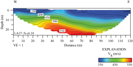
S-wave refraction tomography model for the LA17-5-RUS profile. VS ranges between approximately 300 meters per second (m/s) near the surface and 550 m/s at approximately 25 meters (m) depth. Higher values of VS occur at shallower depths between distance meters approximately 25 and 60 m of the profile. VS is generally higher in the west end of the seismic profile. (W, west; E, east; VE, vertical exaggeration; VS, S-wave velocity.)
MASRW 2-D S-wave Velocity Model
We developed a VS model for the LA17-5-RUS seismic profile by evaluating Rayleigh-waves with the MASW technique. We show a Rayleigh-wave dispersion curve (fig. 1.5A) for the location (meter 0 of our seismic profile) nearest to the SCSN RUS strong-motion recording station. Fundamental mode dispersion curve picks (red circles) correlate with phase velocities between approximately 200 and 800 m/s and frequencies between 2 and 32 Hz. Rayleigh-wave fundamental mode dispersion curve picks for the entire length of the profile (fig. 2.5A) correlate with phase velocities between approximately 200 and 1,300 m/s and frequencies between 2 and 60 Hz. A Rayleigh-wave 1-D depth-velocity profile (fig. 3.5A) nearest to the SCSN LCG strong-motion recording station shows a gradual increase in VS at all depths. We calculated (a) VS30 to be 305 m/s nearest to the SCSN LCG strong-motion recording station, (b) VS30 at each meter along the profile to be between 310 and 330 m/s, and (c) the average VS30 along the entire profile to be 310 m/s (table 3).
We also developed a 2-D MASRW VS model along the seismic profile LA17-5-RUS (fig. 24A) using Rayleigh-waves. Our model shows VS ranges between approximately 200 m/s near the surface and approximately 650 m/s at 40 m depth. Our model shows VS ranges between 200 and 350 m/s in the upper 25 m of the subsurface with a higher gradient below approximately 25 m depth. VS is higher at both the west and east ends of the profile at depths below approximately 10 m.
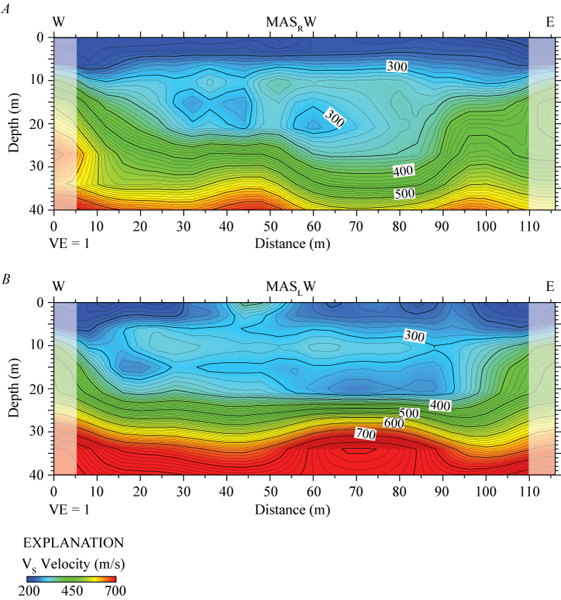
Two-dimensional MASRW and MASLW shear-wave velocity models for profile LA17-5-RUS. A, Our MASRW-derived VS ranges between approximately 200 meters per second (m/s) near the surface and approximately 650 m/s at approximately 40 meters (m) depth. B, Two-dimensional MASLW model (derived from a 3.5-kg sledgehammer and aluminum block source) indicates VS ranges between approximately 250 m/s near the surface and approximately 800 m/s at 40 m depth. Both MASW-based models show VS to be between 250 and 400 m/s in the upper 20 m of the subsurface, with higher VS gradients below 20 m. Shaded areas represent regions with few data points. (W, west; E, east; VE, vertical exaggeration; VS, S-wave velocity.)
MASLW 2-D S-wave Velocity Model—3.5-kg Sledgehammer Source
We developed a Love-wave dispersion curve (fig. 1.5B) for the location (meter 0 on our seismic profile) nearest to the SCSN RUS strong-motion recording station. Fundamental mode dispersion curve picks (red circles) correlate with phase velocities between approximately 150 and 800 m/s and frequencies between 2 and 24 Hz. Love-wave fundamental mode dispersion curve picks along the entire profile (fig. 2.5B) correlate with phase velocities between approximately 150 and 1,200 m/s and frequencies between 2 and 40 Hz. The Love-wave 1-D depth-velocity profile (fig. 3.5B) nearest to the SCSN RUS strong-motion recording station shows a gradual increase in VS below approximately 2 m depth. We calculated (a) VS30 to be 351 m/s nearest to the SCSN RUS strong-motion recording station, (b) VS30 at each meter along the profile to be between 288 and 351 m/s, and (c) the average VS30 across the entire profile to be 308 m/s (table 3).
We developed a 2-D MASLW VS model along the LA17-5-RUS seismic profile (fig. 24B). Our model shows VS ranges between approximately 250 m/s near the surface and approximately 800 m/s at 40 m depth. Our model shows VS ranges between 200 and 350 in the upper 20 m of the subsurface, with a relatively higher gradient below 20 m depth. VS is generally higher at both west and east ends of the seismic profile at depths below approximately 10 m.
Profile LA17-6—Santa Clara (SCSN STC)
P-wave Refraction Tomography (VP) Model
We developed a refraction tomography P-wave velocity model from first arrival refractions. In our model, VP ranges between approximately 350 m/s near the surface and approximately 1400 m/s at 45 m depth (fig. 25). Velocity contours are generally sub-horizontal along the entire seismic profile at all depths in the upper 45 m of the subsurface. The SCSN STC strong-motion recording station was located approximately 240 m northwest of our seismic profile and nearest to distance meter 120 of our profile.
P-wave refraction tomography model for profile LA17-6-STC. P-wave velocities range between approximately 350 meters per second (m/s) near the surface and 1,400 m/s at approximately 45 meters (m) depth. (SE, southeast; NW, northwest; VE, vertical exaggeration; VP, P-wave velocity.)
S-wave Refraction Tomography (VS) Model
We developed an S-wave refraction tomography model from first-arrival shear-waves. Our model shows that VS ranges between approximately 300 m/s near the surface and approximately 700 m/s at 25 m depth (fig. 26). VS contours are generally sub-parallel between distance meters 0 and approximately 65 along the profile. We calculated VS30 at every meter along the profile to be between 372 and 504 m/s and calculated VS30 nearest to the SCSN STC strong-motion station (near distance meter 120 of our seismic profile) to be 377 m/s (table 3).
S-wave refraction tomography model for the LA17-6-STC seismic profile. VS ranges between approximately 300 meters per second (m/s) near the surface and 700 m/s at approximately 25 meters (m) depth. VS is generally lower near the northwest half of the seismic profile. (SE, southeast; NW, northwest; VE, vertical exaggeration; VS, S-wave velocity.)
MASRW 2-D S-wave Velocity Model
We developed a Rayleigh-wave dispersion curve (fig. 1.6A) for the location nearest to the SCSN STC strong-motion recording station (meter 120 of our seismic profile). Fundamental mode dispersion curve picks (red circles) correlate with phase velocities between approximately 200 and 500 m/s and frequencies between 4 and 60 Hz. Rayleigh-wave fundamental mode dispersion curve picks along the entire length of the profile (fig. 2.6A) generally correlate at phase velocities between approximately 150 and 1,400 m/s and frequencies between 2 and 70 Hz. The Rayleigh-wave 1-D depth-velocity profile (fig. 3.6A) nearest to the SCSN STC strong-motion recording station indicates a gradual increase in VS below approximately 8 m depth. We calculated (a) VS30 to be 311 m/s nearest to the SCSN STC strong-motion recording station, (b) VS30 at each meter along the profile to range between 269 and 318 m/s, and (c) the average VS30 along the entire profile to be 294 m/s (table 3).
We developed a VS model for the LA17-6-STC seismic profile by evaluating Rayleigh-waves with the MASW technique. Our 2-D MASRW VS model along the seismic profile LA17-6-STC (fig. 27A) shows VS ranges between approximately 180 m/s near the surface and approximately 550 m/s at 40 m depth. Our VS model shows a channel-like velocity structure below approximately 10 m depth between distance meters approximately 40 and 80. A smaller channel-like velocity structure is also observed between distance meters 90 and 105. VS is higher near both the southeast and northwest ends of the profile at depths below approximately 12 m.
Two-dimensional MASRW- and MASLW-derived VS models for profile LA17-6-STC. A, Our MASRW model indicates VS ranges between approximately 180 meters per second (m/s) near the surface and approximately 550 m/s at approximately 40 meters (m) depth. B, Our MASLW model was derived from data generated by 3.5-kilogram sledgehammer and aluminum block source. VS, derived from the MASLW data, ranges between approximately 200 m/s near the surface and approximately 450 m/s at 40 m depth. Both multichannel analysis of surface waves models show channel-like velocity structures near the middle of the profile, between distance meters approximately 40 and approximately 90. Shaded areas represent regions with few data points. (SE, southeast; NW, northwest; VE, vertical exaggeration; VS, S-wave velocity.)
MASLW 2-D S-wave Velocity Model—3.5-kg Sledgehammer Source
We present a Love-wave dispersion curve (fig. 1.6B) for the location (meter 120 of our seismic profile) nearest to the SCSN STC strong-motion recording station. Fundamental mode dispersion curve picks (red circles) correlate with phase velocities between approximately 200 and 600 m/s and frequencies between 3 and 55 Hz. Love-wave fundamental mode dispersion curve picks along the entire length of the profile (fig. 2.6B) generally correlate with phase velocities between approximately 150 and 1,300 m/s and frequencies between 2 and 80 Hz. Our Love-wave 1-D depth-velocity profile (fig. 3.6B) nearest to the SCSN STC strong-motion recording station shows a gradual increase in VS between approximately 2 and 40 m depth. We calculated (a) VS30 to be 330 m/s nearest to the SCSN STC strong-motion recording station, (b) VS30 at each meter along the profile to be between 302 and 331 m/s, and (c) the average VS30 across the entire profile to be 320 m/s (table 3).
We developed a 2-D MASLW VS model along the seismic profile LA17-6-STC (fig. 27B). Our model shows VS ranges between approximately 200 m/s near the surface and approximately 450 m/s at 40 m depth. Our VS MASLW-derived model shows a channel-like velocity structure below approximately 10 m depth between distance meters approximately 45 and 95. VS is generally higher near both the southeast and northwest ends of the seismic profile at depths below approximately 10 m.
VP/VS Ratios
The ratio of P-wave velocities to S-wave velocities (VP/VS) can provide information about the physical state and lithology of subsurface materials (Tatham, 1982; Castagna and others, 1985). We derived VP/VS models for each of the six seismic profiles (appendix 4) in this report by dividing VP by the VS at each node of the refraction tomography models. VP/VS ratios range between 1 and 3 in all six seismic profiles. VP/VS ratios along the LA17-1-OLI seismic profile range between approximately 1.3 and 2.6, with the highest VP/VS ratios (more than 2) occurring in the upper 5 m of the subsurface (fig. 4.1). VP/VS ratios along the LA17-2-SRN seismic profile range between approximately 1.2 and 2, with the highest VP/VS ratios (approximately 2) forming a southwest-dipping feature between distance meters 110 and 170, which coincides with the approximate mapped trace of the Peralta Hills Fault (fig. 4.2). VP/VS ratios along the LA17-3-MUR seismic profile range between 1 and 2, with the highest ratios (approximately 2) occurring at depths below approximately 25 m between distance meters 65 and 95 and occurring at discrete locations at varying depths between distance meters 45 and 105 (fig. 4.3). VP/VS ratios along the LA17-4-LCG seismic profile range between 1.4 and 2.6, with the highest ratios (more than 2) occurring near the south end of the profile in the upper 10 m of the subsurface and at depths below approximately 10 m between distance meters 40 and 115 (fig. 4.4). VP/VS ratios along the LA17-5-RUS seismic profile range between 1 and 3.5, with the highest ratios occurring at depths below approximately 15 m (fig. 4.5). Finally, VP/VS ratios along the LA17-6-STC seismic profile range between 1 and 1.6, with the highest ratios (approximately 1.6) occurring at depths below approximately 15 to 20 meters between distance meters 70 and 100 (fig. 4.6).
Poisson’s Ratios
Poisson’s ratios provide information about water-saturation levels and clay content of the soil in subsurface materials (Castagna and others, 1985; Catchings and others, 2006), whereby relatively high Poisson’s ratios above 0.44 (determined from tomographic seismic data) typically coincide with the top of groundwater (Catchings and others, 2006; 2014). We developed Poisson’s ratio models from refraction tomographic VP and VS models using the calculation determined by Thomsen (1990). These models are presented in appendix 5 of this report.
Poisson’s ratios along the LA17-1-OLI seismic profile range between approximately 0.02 and 0.4. The highest Poisson’s ratios (approximately 0.4) occur in the upper meter of the subsurface, which may suggest near-surface saturated materials or materials with high clay content on the berm (fig. 5.1). Poisson’s ratios along the LA17-2-SRN seismic profile range between approximately 0.025 and 0.325. The highest Poisson’s ratios (more than 0.3) occur below approximately 5 m depth between distance meters 110 and 155 (fig. 5.2). Whereas Poisson’s ratios along the profile are inconsistent with saturated materials, the highest Poisson’s ratios coincide with a mapped trace of the Peralta Hills Fault, which indicates fluid accumulation along the fault. Poisson’s ratios along the LA17-3-MUR seismic profile range between approximately 0.1 and 0.325, with highest Poisson’s ratios (more than 0.3) occurring at discreet locations and varying depths along the profile (fig. 5.3). Poisson’s ratios along the LA17-4-LCG seismic profile range between approximately 0.05 and 0.375, with highest Poisson’s ratios (more than 0.35) occurring below approximately 5 m depth between distance meters 25 and 120 and extending to the surface between distance meters 0 and 10 (fig. 5.4). Poisson’s ratios along the LA17-5-RUS seismic profile range between 0.05 and 0.45, with highest ratios (more than 0.45) occurring in a near-horizontal zone at approximately 15 m depth, which suggest the presence of saturated materials or clay (fig. 5.5). Poisson’s ratios along the LA17-6-STC seismic profile range between approximately 0.05 and 0.22. The highest ratios (more than 0.2) occur below approximately 20 m depth between distance meters 70 and 100 (fig. 5.6).
Summary
The USGS evaluated VS at six strong-motion recording stations in Southern California Edison substations to better understand the potential for amplified ground shaking during an earthquake. Prior site-characterization studies in California show some sites exhibit considerable lateral variability in shear-wave velocities due to complex geologic structures at depth. We used refraction tomography and MASW methods to evaluate the 2-D VS from body and surface waves data recorded along linear profiles generated by active-source seismic methods. We calculated VS30 at every meter along the linear profiles and compared results between the different methods of analysis.
VS and VS30 Comparisons
Profile LA17-1—Olinda (SCSN OLI)
S-wave refraction tomography, MASRW, and MASLW models all show slightly higher VS in the west side of the LA17-1-OLI profile, whereas the surface-wave models show a channel-like velocity structure centered near distance meter 130 near the east end of the profile. Orthoimagery (fig. 2) indicates a stream (culvert) may have been rerouted around the eastern portion of the substation. The average VS30 values for the profile (table 3), calculated from S-wave refraction tomography, MASRW, and MASLW (sledgehammer and 45°-angle AWD methods), are 334 meters per second (m/s), 291 m/s, 289 m/s, and 309 m/s, respectively. The various methods show only a 45 m/s difference in VS30 values. At the point on the seismic profile nearest to the strong-motion recording station, VS30 values, calculated from S-wave refraction tomography, MASRW, and MASLW (sledgehammer and 45°-angle AWD) methods, are 320 m/s, 371 m/s, 494 m/s, and 410 m/s, respectively. The various methods show up to a 174 m/s difference (table 3) in VS30 values for the location of the profile nearest to the strong-motion recording station, with the greatest difference occurring between VS30 derived from the S-wave refraction tomography and MASLW methods. Calculated using surface wave methods, the average VS30 along the seismic profile nearest to the strong-motion recording station are up to 205 m/s higher than the average VS30 for the entire seismic profile, suggesting significant lateral VS variability across the recording site.
Profile LA17-1b—Olinda (SCSN OLI)
Our MASRW-derived VS model shows slightly higher VS at the southern part of the LA17-1b-OLI profile between distance meters 0 and 45 (fig. 12). The average VS calculated for the entire profile is 309 m/s, whereas VS calculated at the point nearest to the recording station is 330 m/s. VS30 calculated at every meter along the profile in the north-south direction is smaller in range than those calculated for the west-to-east direction (table 3), which suggests variation in VS is smaller in the north-to-south direction.
Profile LA17-2—Serrano (SCSN SRN)
S-wave refraction tomography, MASRW, and MASLW models all show undulating velocity contours, which suggest complex geologic structures at depth (figs. 14 and 15). The Peralta Hills Fault has been mapped as crossing the substation and our seismic profile at approximately distance meters 160–165; our VP/VS and Poisson’s ratios are highest at the same general location, which corroborates the mapped trace of the fault (figs. 4.2 and 5.2). The average VS30 for the profile (table 3), calculated from S-wave refraction tomography, MASRW, and MASLW (sledgehammer and 45°-angle AWD) methods, are 542 m/s, 383 m/s, 444 m/s, and 462 m/s, respectively (a range of 159 m/s). VS30, calculated from S-wave refraction tomography, MASRW, and MASLW (sledgehammer and 45°-angle AWD) methods at the point on the seismic profile nearest to the strong-motion recording station, are 537 m/s, 379 m/s, 432 m/s, and 443 m/s, respectively (a range of 158 m/s). The difference between the average VS30 values calculated for the entire seismic profile and VS30 calculated at the point nearest to the strong-motion recording station is minor (difference up to 19 m/s). Overall, the difference between minimum and maximum VS30 values along the seismic profile ranges between 51 and 118 m/s, with VS30 calculated from the S-wave refraction tomography method having the largest range and higher values than those calculated using surface wave methods. We attribute the differences observed among the different models to the surface wave methods’ difficulty in resolving complex bedrock structures at shallow depths.
Profile LA17-3—Murrieta (SCSN MUR)
S-wave refraction tomography and MASRW models both show higher VS in the northeast end of the LA17-3-MUR profile, between distance meters 40 and 100 (S-wave refraction tomography) and between distance meters 85 and 110 (MASRW). Surface-wave models show more significant undulating velocity contours, which may suggest complex geologic structures in the subsurface; however, there is significant topographic variation along the profile, which causes difficulty for the 1-D surface-wave methods. The average VS30 values for the profile, calculated from S-wave refraction tomography, MASRW, and MASLW (sledgehammer and 45°-angle AWD) methods, are 685 m/s, 592 m/s, 463 m/s, and 491 m/s, respectively. VS30 values (table 3), calculated from S-wave refraction tomography, MASRW, and MASLW (sledgehammer and 45°-angle AWD) methods at the point on the seismic profile nearest to the strong-motion recording station, are 497 m/s, 613 m/s, 318 m/s, and 318 m/s, respectively. The average VS30 calculated for the seismic profile varies by as much as 188 m/s from VS30 calculated nearest to the strong-motion recording station, which suggests lateral VS variability due to complex geological structures and a change in surface topography. Overall, the difference between minimum and maximum VS30 values across the seismic profiles among different methods range between 94 and 272 m/s, with VS30 values calculated from the S-wave refraction tomography method having the largest range. This quality of the S-wave refraction tomography method is generally consistent across the different sites in this study.
Profile LA17-4—La Cienega (SCSN LCG)
S-wave refraction tomography and MASRW-based models for the LA17-4-LCG profile indicate relatively higher VS at depths below approximately 15 meters (m) at distance meters between 0 and 45 (S-wave refraction tomography) and at distance meters between 8 and 25 (MASRW). However, our MASLW-based model shows a channel-like structure, whereas both S-wave refraction tomography and MASRW models show higher VS at depth. Undulating velocity contours seen in all three models may suggest complex geological structures at depth (figs. 20 and 21). The Newport-Inglewood-Rose Canyon Fault Zone has been mapped (fig. 5) less than 200 m northeast of our seismic profile, further suggesting structural complexity at this location. The average VS30 values for the profile (table 3), calculated from S-wave refraction tomography, MASRW, and MASLW methods, are 660 m/s, 374 m/s, and 555 m/s, respectively. VS30, calculated from S-wave refraction tomography, MASRW, and MASLW methods at the point on the seismic profile nearest to the strong-motion recording station are 595 m/s, 425 m/s, and 645 m/s, respectively. The average VS30 calculated for the seismic profile varies by as much as 90 m/s from VS30 calculated nearest to the strong-motion recording station, which suggests lateral VS variability due to complex geological structures at depth. Overall, the difference between minimum and maximum VS30 along the seismic profile ranges between 69 and 256 m/s, with VS30 calculated from the S-wave refraction tomography method having the largest range. In general, Vs determined from the S-wave refraction tomography method is higher than VS determined from surface-wave methods at this location.
Profile LA17-5—Rush (SCSN RUS)
Our S-wave refraction tomography model shows higher VS in the western part of the seismic profile between distance meters 0 and approximately 50, whereas our surface-wave models show higher VS in both the west and east ends of the profile (figs. 23 and 24). The surface-wave models show VS is generally less than 350 m/s in the upper approximately 20 m of the subsurface between distance meters 25 and 90 (MASRW) and between distance meters 10 and 100 (MASLW), with high VS gradients from approximately 20 m depth to the bottom of the models at 40 m. The average VS30 values for the profile (table 3), calculated from S-wave refraction tomography, MASRW, and MASLW methods, are 448 m/s, 310 m/s, and 308 m/s, respectively. VS30 measurements, calculated from the S-wave refraction tomography, MASRW, and MASLW methods at the point on the seismic profile nearest to the strong-motion recording station, are 468 m/s, 305 m/s, and 351 m/s, respectively. The average VS30 calculated from the seismic profile varies as much as 43 m/s from VS30 calculated nearest to the strong-motion recording station. Overall, the difference between minimum and maximum VS30 along the seismic profile ranges between 20 and 97 m/s, with VS30 calculated from S-wave refraction tomography having the largest range.
Profile LA17-6—Santa Clara (SCSN STC)
Our S-wave refraction tomography, MASRW, and MASLW models all show higher VS in the southeastern part of the seismic profile; however, our surface-wave models show channel-like velocity structures between distance meters 40 and 100 (figs. 26 and 27). The average VS30 values for the profile (table 3), calculated from S-wave refraction tomography, MASRW, and MASLW methods, are 443 m/s, 294 m/s, and 320 m/s, respectively. VS30, calculated from S-wave refraction tomography, MASRW, and MASLW methods at the point on the seismic profile nearest to the strong-motion recording station, are 377 m/s, 311 m/s, and 330 m/s, respectively. Overall, the difference between minimum and maximum VS30 along the seismic profile ranges between 29 and 132 m/s, with VS30 calculated from S-wave refraction tomography having the largest and highest ranges relative to those calculated from surface-wave methods.
Method Comparison
We find varying magnitudes of differences in VS30 among all methods (refraction tomography, Rayleigh-wave MASRW, and Love-wave MASLW) when the site contains surface topography, shallow bedrock, and (or) complex geologic structures at depth. Our prior studies (Chan and others, 2018a; 2018b) indicate 2-D S-wave refraction tomography is better at resolving complex sites, while both body- and surface wave methods perform similarly at sites without topography and (or) bedrock. Furthermore, we expect varying VS in our surface wave models due to non-uniqueness of inversion results and the challenges of wave propagation in weathered bedrock (Garofalo and others, 2016a; 2016b; Ladak and others, 2021).
References Cited
Baltay, A.S., and Boatwright, J., 2015, Ground-motion observations of the 2014 south Napa earthquake: Seismological Research Letters, v. 86, no. 2A, p. 355–360, https://doi.org/10.1785/0220140232.
Castagna, J.P., Batzle, M.L., and Eastwood, R.L., 1985, Relationships between compressional-wave and shear-wave velocities in clastic silicate rocks: Geophysics, v. 50, no. 4, p. 571–581, https://doi.org/10.1190/1.1441933.
Catchings, R.D., Addo, K.O., Goldman, M.R., Chan, J.H., Sickler, R.R., and Criley, C.J., 2019, Two-dimensional seismic velocities and structural variations at three British Columbia Hydro and Power Authority (BC Hydro) dam sites, Vancouver Island, British Columbia, Canada: U.S. Geological Survey Open-File Report 2019–1015, 137 p., https://doi.org/10.3133/ofr20191015.
Catchings, R.D., Borchers, J.W., Goldman, M.R., Gandhok, G., Ponce, D.A., and Steedman, C.E., 2006, Subsurface structure of the East Bay plain ground-water basin—San Francisco Bay to the Hayward Fault, Alameda County, California: U.S. Geological Survey Open-File Report 2006–1084, 61 p., https://doi.org/10.3133/ofr20061084.
Catchings, R.D., Gandhok, G., Goldman, M.R., Okaya, D., 2001, Seismic images and fault relations of the Santa Monica Thrust Fault, West Los Angeles, California: U.S. Geological Survey Open-File Report 01–111, 34 p., https://doi.org/10.3133/ofr01111.
Catchings, R.D., Goldman, M.R., Trench, D., Buga, M., Chan, J.H., Criley, C.J., and Strayer, L.M., 2017, Shallow-depth location and geometry of the Piedmont Reverse splay of the Hayward Fault, Oakland, California: U.S. Geological Survey Open-File Report 2016–1123, 22 p., https://doi.org/10.3133/ofr20161123.
Catchings, R.D., Rymer, M.J., Goldman, M.R., Prentice, C.S., and Sickler, R.R., 2013, Fine-scale delineation of the location of and relative ground shaking within the San Andreas Fault zone at San Andreas Lake, San Mateo County, California: U.S. Geological Survey Open-File Report 2013–1041, 53 p., https://doi.org/10.3133/ofr20131041.
Catchings, R.R., Rymer, M.J., Goldman, M.R., Sickler, R.R., and Criley, C.J., 2014, A method and example of seismically imaging near-surface fault zones in geologically complex areas using VP, VS, and their ratios: Bulletin of the Seismological Society of America, v. 104, no. 4, p. 1989–2006, https://doi.org/10.1785/0120130294.
Chan, J.H., Catchings, R.D., Goldman, M.R., and Criley, C.J., 2018a, VS30 at three strong-motion recording stations in Napa and Napa County, California—Main Street in downtown Napa, Napa fire station number 3, and Kreuzer Lane—Calculations determined from S-wave refraction tomography and multichannel analysis of surface waves (Rayleigh and Love): U.S. Geological Survey Open-File Report 2018–1161, 47 p., https://doi.org/10.3133/ofr20181161.
Chan, J.H., Catchings, R.D., Goldman, M.R., and Criley, C.J., 2018b, VS30 at three strong-motion recording stations in Napa and Solano Counties, California—Lovall Valley Road, Broadway Street and Sereno Drive in Vallejo, and Vallejo Fire Station—Calculations determined from S-wave refraction tomography and multichannel analysis of surface waves (Rayleigh and Love): U.S. Geological Survey Open-File Report 2018–1162, 62 p., https://doi.org/10.3133/ofr20181162.
Chan, J.H., Catchings, R.D., Goldman, M.R, Criley, C.J., and Sickler, R.R., 2021, High-resolution seismic data acquired at six Southern California seismic network (SCSN) recording stations in 2017: U.S. Geological Survey data release, https://doi.org/10.5066/P990O55F.
Garofalo, F., Foti, S., Hollender, F., Bard, P.Y., Cornou, C., Cox, B.R., Ohrnberger, M., Sicilia, D., Asten, M., Di Giulio, G., Forbriger, T., Guillier, B., Hayashi, K., Martin, A., Matsushima, S., Mercerat, D., Poggi, V., and Yamanaka, H., 2016a, InterPACIFIC project—Comparison of invasive and non-invasive methods for seismic site characterization—Part I—Intra-comparison of surface-wave methods: Soil Dynamics and Earthquake Engineering, v. 82, p. 222–240, https://doi.org/10.1016/j.soildyn.2015.12.010.
Garofalo, F., Foti, S., Hollender, F., Bard, P.Y., Cornou, C., Cox, B.R., Dechamp, A., Ohrnberger, M., Perron, V., Sicilia, D., Teague, D., and Vergniault, C., 2016b, InterPACIFIC project—Comparison of invasive and non-invasive methods for seismic site characterization—Part II—Inter-comparison between surface-wave and borehole methods: Soil Dynamics and Earthquake Engineering, v. 82, p. 241–254, https://doi.org/10.1016/j.soildyn.2015.12.009.
Hayashi, K., and Hikima, K., 2003, CMP analysis of multi-channel surface wave data and its application to near-surface s-wave velocity delineation, in Symposium on the Application of Geophysics to Engineering and Environmental Problems (SAGEEP), 15th, San Antonio, Tex., April 2003: Denver, Colo., SAGEEP, p. 1348–1355.
Hayashi, K., and Suzuki, H., 2004, CMP cross-correlation analysis of multi-channel surface-wave data: Exploration Geophysics, v. 35, no. 1, p. 7–13, https://doi.org/10.1071/EG04007.
Hole, J.A., 1992, Nonlinear high-resolution three-dimensional seismic travel time tomography: Journal of Geophysical Research, v. 97, no. B5, p. 6553–6562, https://doi.org/10.1029/92JB00235.
Holtzer, T.L., Padovani, A.C., Bennett, M.J., Noce, T.E., Tinsley, J.C., 2005, Mapping NEHRP VS30 site classes: Earthquake Spectra, v. 21, no. 2, p. 1–18, https://doi.org/10.1193/1.1895726.
Ivanov, J., Leitner, B., Shefchik, W., Shwenk, J.T., and Peterie, S.L., 2013, Evaluating hazards at salt cavern sites using multichannel analysis of surface waves: Leading Edge, v. 32, no. 3, p. 298–305, https://doi.org/10.1190/tle32030298.1.
Park, C., 2013, MASW for geotechnical site investigation: Leading Edge, v. 32, no. 6, p. 656–662, https://doi.org/10.1190/tle32060656.1.
Park, C., Miller, R., and Xia, J., 1999, Multichannel analysis of surface waves: Geophysics, v. 64, no. 3, p. 800–808, https://doi.org/10.1190/1.1444590.
Park, C., Miller, R., Xia, J., and Ivanov, J., 2007, Multichannel analysis of surface waves (MASW)—Active and passive methods: Leading Edge, v. 26, no. 1, p. 60–64, https://doi.org/10.1190/1.2431832.
Pujol, J., 2003, Elastic wave propagation and generation in seismology: Cambridge University Press, United Kingdom, https://doi.org/10.1017/CBO9780511610127.
Tatham, R.H., 1982, Vp/Vs and lithology: Geophysics, v. 47, p. 336–344, https://doi.org/10.1190/1.1441339.
Thomsen, L., 1990, Poisson was not a geophysicist!: Leading Edge, v. 9, no. 12, p. 27–29, https://doi.org/10.1190/1.1439706.
U.S. Geological Survey National Geospatial Program, 2009, The National Map-Orthimagery: U.S. Geological Survey, accessed March 1, 2022, at https://apps.nationalmap.gov/viewer/.
U.S. Geological Survey Earthquake Hazards Program, 2020, Quaternary fault and fold database for the United States: U.S. Geological Survey, accessed March 1, 2021, at https://www.usgs.gov/natural-hazards/.
Xia, J., Miller, R.D., and Park, C.B., 1999, Estimation of near-surface shear-wave velocity by inversion of Rayleigh waves: Geophysics, v. 64, no. 3, p. 691–700, https://doi.org/10.1190/1.1444578.
Xia, J., Miller, R., Park, C., and Ivanov, J., 2000, Construction of 2-D vertical shear wave velocity field by the multichannel analysis of surface wave technique, in Symposium on the application of geophysics to engineering and environmental problems 2000: Environment and Engineering Geophysical Society, Symposium on the Application of Geophysics to Engineering and Environmental Problems, p. 1197–1206, https://doi.org/10.4133/1.2922726.
Yong, A., Martin, A., Stokoe, K., and Diehl, J., 2013, ARRA-funded VS30 measurements using multi-technique approach at strong-motion stations in California and Central-Eastern United States: U.S. Geological Survey Open-File Report 2013–1102, 60 p., https://doi.org/10.3133/ofr20131102.
Zeng, C., Xia, J., Miller, R.D., Tsoflias, G.P., and Wang, Z., 2012, Numerical investigation of MASW applications in the presence of surface topography: Journal of Applied Geophysics, v. 84, p. 52–60, https://doi.org/10.1016/j.jappgeo.2012.06.004.
Appendix 1. Rayleigh- and Love-Wave Dispersion Curves Nearest to Strong-Motion Recording Station
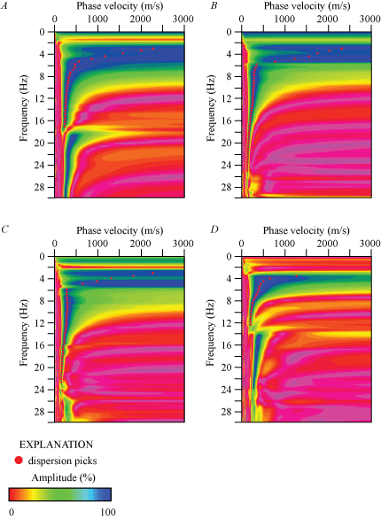
Rayleigh- and Love-wave dispersion curves correlating with points on our LA17-1-OLI and LA17-1b-OLI seismic profiles that are nearest to the SCSN OLI strong-motion station. A, The Rayleigh-wave fundamental mode dispersion curve is between 2 and 17 hertz (Hz). Dispersion curve picks (red circles) correlate with phase velocities between 250 and 2,300 meters per second (m/s). B, Dispersion curve developed from data generated by a 3.5-kilogram sledgehammer and aluminum block source. Love-wave fundamental mode dispersion curve between 2 and 26 Hz. Dispersion curve picks (red circles) are between approximately 250 and 2,300 m/s. C, Dispersion curve developed from data generated by a 45°-angle accelerated weight-drop and aluminum block source. Love-wave fundamental mode dispersion curve between 2 and 24 Hz. Dispersion curve picks (red circles) correlate with phase velocities between 250 and 2,300 m/s. D, A Rayleigh-wave fundamental mode dispersion curve for the LA17-1b-OLI seismic profile is distinct from higher modes between 3 and 12 Hz. Dispersion curve picks (red circles) correlate with phase velocities between approximately 250 and 1,400 m/s.
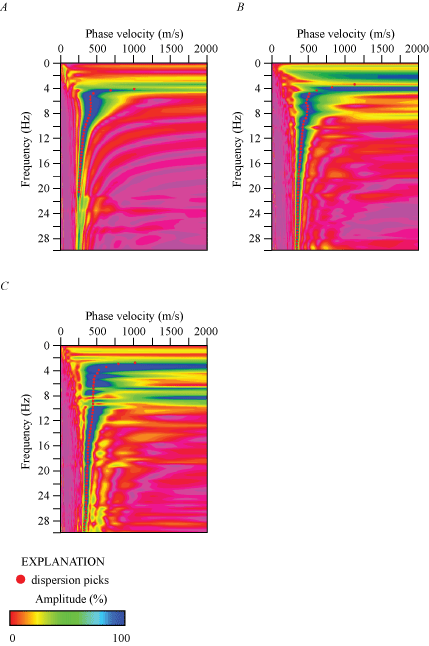
Rayleigh- and Love-wave dispersion curves corresponding to the location along our LA17-2-SRN seismic profile that is nearest to the SCSN SRN strong-motion station. A, A Rayleigh-wave fundamental mode dispersion curve for frequencies between 4 and 22 hertz (Hz). Dispersion curve picks (red circles) correlate with phase velocities between approximately 250 and 1,000 meters per second (m/s). B, Dispersion curve developed from data generated by a 3.5-kilogram sledgehammer and aluminum block source. Love-wave fundamental mode dispersion curve for frequencies between 2 and 30 Hz. Dispersion curve picks (red circles) correlate with velocities of approximately 250 and 1,200 m/s. C, Dispersion curve developed from data generated by a 45°-angle accelerated weight-drop and aluminum block source. This is a Love-wave fundamental mode dispersion curve for frequencies between 2 and 30 Hz. Dispersion curve picks (red circles) correlate with phase velocities between approximately 250 and 1,100 m/s.
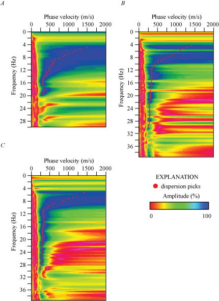
Rayleigh- and Love-wave dispersion curves corresponding to the location on our LA17-3-MUR seismic profile that is nearest to the SCSN MUR strong-motion station. A, Rayleigh-wave fundamental mode dispersion curve for frequencies between 4 and 20 hertz (Hz). Dispersion curve picks (red circles) correlate with phase velocities between 250 and 1,500 meters per second (m/s). B, Dispersion curve developed from data generated by a 3.5-kilogram sledgehammer and aluminum block source. Love-wave fundamental mode dispersion curve for frequencies between 4 and 32 Hz. Dispersion curve picks (red circles) correlate with phase velocities between 250 and 1,500 m/s. C, Dispersion curve developed from data generated by a 45°-angle accelerated weight-drop and aluminum block source. Love-wave fundamental mode dispersion curve for frequencies between 4 and 32 Hz. Dispersion curve picks (red circles) correlating with phase velocities between 250 and 1,500 m/s.
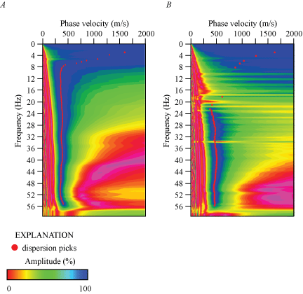
Rayleigh- and Love-wave dispersion curves corresponding to the location on our LA17-4-LCG seismic profile that is nearest to the SCSN LCG strong-motion station. A, Rayleigh-wave fundamental mode dispersion curve for frequencies between 2 and 56 hertz (Hz). Dispersion curve picks (red circles) correlating with phase velocities between 250 and 1,600 meters per second (m/s). B, Dispersion curve developed from data generated by a 3.5-kilogram sledgehammer and aluminum block source. The Love-wave fundamental mode dispersion curve for frequencies between 2 and 56 Hz. Dispersion curve picks (red circles) correlating with phase velocities between 250 and 1,600 m/s.
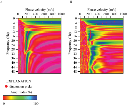
Rayleigh- and Love-wave dispersion curves corresponding to the location along our profile LA17-5-RUS seismic profile that is nearest to the SCSN RUS strong-motion station. A, Rayleigh-wave fundamental mode dispersion curve for frequencies between 2 and 32 hertz (Hz). Dispersion curve picks (red circles) correlating with phase velocities between 200 and 800 meters per second (m/s). B, Dispersion curve picks developed from data generated by a 3.5-kilogram sledgehammer and aluminum block source. Love-wave fundamental mode dispersion curve for frequencies between 2 and 24 Hz. Dispersion curve picks (red circles) correlate with phase velocities between 150 and 800 m/s.
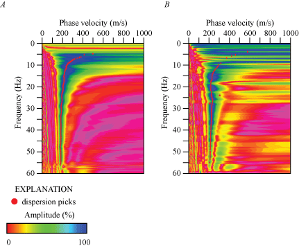
Rayleigh- and Love-wave dispersion curves corresponding to the location on our LA17-6-STC seismic profile that is nearest to the SCSN STC strong-motion station. A, Rayleigh-wave fundamental mode dispersion curve for frequencies between 4 and 60 hertz (Hz). Dispersion curve picks (red circles) correlate with phase velocities between 200 and 500 meters per second (m/s). B, Dispersion curve developed from data generated by a 3.5-kilogram sledgehammer and aluminum block source. Love-wave fundamental mode dispersion curve for frequencies between 3 and 55 Hz. Dispersion curve picks (red circles) correlate with phase velocities between 200 and 600 m/s.
Appendix 2. Rayleigh- and Love-Wave Fundamental mode Dispersion Curve Picks
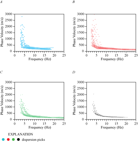
Rayleigh- and Love-wave fundamental mode dispersion curve picks for our LA17-1-OLI and LA17-1b-OLI seismic profiles. A, Rayleigh-wave fundamental mode dispersion curve picks correlate with frequencies between 3 and 20 hertz (Hz) and with phase velocities between 200 and 2,500 meters per second (m/s). B, Dispersion curves developed from data generated by a 3.5-kilogram sledgehammer and aluminum block source. Love-wave fundamental mode dispersion curve picks for frequencies between 2 and 25 Hz and phase velocities between 200 and 2,500 m/s. C, Dispersion curves developed from data generated by a 45°-angle accelerated weight-drop and aluminum block source. Love-wave fundamental mode dispersion curve picks for frequencies between 2 and 25 Hz and phase velocities between 200 and 2,000 m/s. D, Rayleigh-wave fundamental mode dispersion curve picks from data along the LA17-1b-OLI profile for frequencies 3 and 21 Hz and phase velocities between 200 and 1,500 m/s.
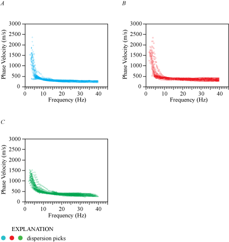
Rayleigh- and Love-wave fundamental mode dispersion curve picks for our LA17-2-SRN seismic profile. A, Rayleigh-wave fundamental mode dispersion curve picks correlate with frequencies between 2 and 40 hertz (Hz) and with phase velocities between 250 and 2,500 meters per second (m/s). B, Dispersion curves developed from data generated by a 3.5-kilogram sledgehammer and aluminum block source. Love-wave fundamental mode dispersion curve picks for frequencies between 1 and 40 Hz and phase velocities between 250 and 2,500 m/s. C, Dispersion curves developed from data generated by a 45°-angle accelerated weight-drop and aluminum block source. Love-wave fundamental mode dispersion curve picks for frequencies between 2 and 40 Hz and phase velocities between 250 and 1,600 m/s.
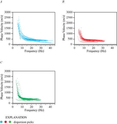
Rayleigh- and Love-wave fundamental mode dispersion curve picks for our LA17-3-MUR seismic profile. A, Rayleigh-wave fundamental mode dispersion curve picks correlate with frequencies between 4 and 45 hertz (Hz) and with phase velocities between 100 and 2,600 meters per second (m/s). B, Dispersion curves developed from data generated by a 3.5-kilogram sledgehammer and aluminum block source. Love-wave fundamental mode dispersion curve picks for frequencies between 3 and 33 Hz and phase velocities between 200 and 1,500 m/s. C, Dispersion curves developed from data generated by a 45°-angle accelerated weight-drop and aluminum block source. Love-wave fundamental mode dispersion curve picks for frequencies between 3 and 30 Hz and phase velocities between 200 and 2,500 m/s.
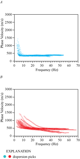
Rayleigh- and Love-wave fundamental mode dispersion curve picks for our LA17-4-LCG seismic profile. A, Rayleigh-wave fundamental mode dispersion curve picks correlate with frequencies between 2 and 56 hertz (Hz) and with phase velocities between 300 and 1,500 meters per second (m/s). B, Dispersion curves developed from data generated by a 3.5-kilogram sledgehammer and aluminum block source. Love-wave fundamental mode dispersion curve picks for frequencies between 2 and 70 Hz and phase velocities between 150 and 1,600 m/s.
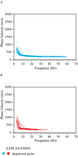
Rayleigh- and Love-wave fundamental mode dispersion curve picks for our LA17-5-RUS seismic profile. A, Rayleigh-wave fundamental mode dispersion curve picks correlate with frequencies between 2 and 60 hertz (Hz) and with phase velocities between 200 and 1,300 meters per second (m/s). B, Dispersion curves developed from data generated by a 3.5-kilogram sledgehammer and aluminum block source. Love-wave fundamental mode dispersion curve picks for frequencies between 2 and 40 Hz and phase velocities between 150 and 1,200 m/s.
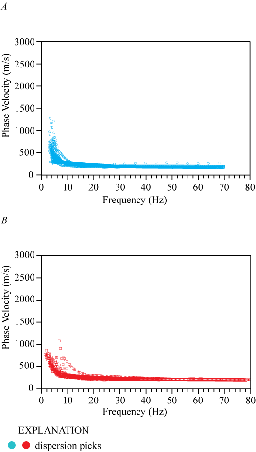
Rayleigh- and Love-wave fundamental mode dispersion curve picks for our LA17-6-STC seismic profile. A, Rayleigh-wave fundamental mode dispersion curve picks correlate with frequencies between 2 and 70 hertz (Hz) and with phase velocities between 150 and 1,400 meters per second (m/s). B, Dispersion curves developed from data generated by a 3.5-kilogram sledgehammer and aluminum block source. Love-wave fundamental mode dispersion curve picks for frequencies between 2 and 80 Hz and phase velocities between 150 and 1,300 m/s.
Appendix 3. Rayleigh- and Love-Wave 1-D Velocity Depth Profiles
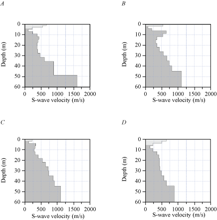
Rayleigh- and Love-wave 1-D depth-velocity profiles correlating with the location along our LA17-1-OLI and LA17-1b-OLI seismic profiles that is nearest to the SCSN OLI strong-motion station. A, Rayleigh-wave 1-D depth-velocity profile showing relatively high gradients below about 30 meters (m) depth. B, Seismic data generated by a 3.5-kilogram sledgehammer and aluminum block source. The Love-wave one-dimensional (1-D) depth-velocity profile shows weak positive gradient in shear-wave velocity (VS) below approximately 10 m depth. C, Dispersion curve developed from data generated by a 45°-angle accelerated weight-drop and aluminum block source. The Love-wave 1-D depth-velocity profile shows weak positive gradient in VS below 10 m depth. D, Rayleigh-wave 1-D depth-velocity profile for the LA17-1b-OLI seismic profile showing a weak positive gradient in VS below approximately 8 m depth. Light grey areas at the near surface represent regions with few data points. (m/s, meters per second.)
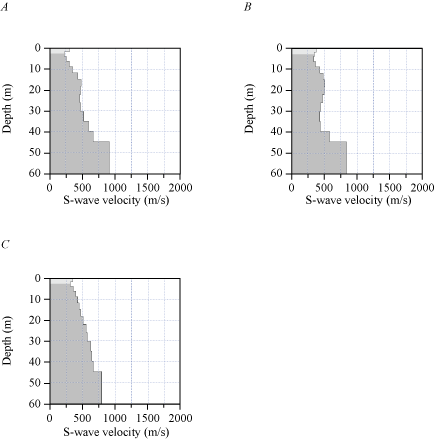
Rayleigh- and Love-wave one-dimensional (1-D) depth-velocity profiles correlating with the location along our LA17-2-SRN seismic profile that is nearest to the SCSN SRN strong-motion station. A, Rayleigh-wave 1-D depth-velocity profile shows positive gradient in shear-wave velocity (VS) below approximately 2 meters (m) depth. B, Seismic data generated by a 3.5-kilogram sledgehammer and aluminum block source. The Love-wave 1-D depth-velocity profile shows weak positive gradient in VS between approximately 2 and approximately 20 m depth, then weak negative gradient in VS between approximately 20 and approximately 40 m depth. C, Seismic data generated by a 45°-angle accelerated weight-drop and aluminum block source. The Love-wave 1-D depth-velocity profile shows weak positive gradient in VS below approximately 2 m depth. Light grey areas at the near surface represent regions with few data points. (m/s, meters per second.)
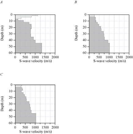
Rayleigh- and Love-wave one-dimensional (1-D) depth-velocity profiles correlating with the location along our LA17-3-MUR seismic profile that is nearest to the SCSN MUR strong-motion station. A, Rayleigh-wave 1-D depth-velocity profile showing positive gradient in shear-wave velocity (VS) between approximately 8 and approximately 18 meters m depth and below approximately 36 m depth. B, Seismic data generated by a 3.5-kilogram sledgehammer and aluminum block source. The Love-wave 1-D depth-velocity profile shows weak positive gradient in VS at all depths. C, Seismic data generated by a 45°-angle accelerated weight-drop and aluminum block source. The Love-wave 1-D depth-velocity profile shows weak positive gradient in VS at all depths. Light grey areas at the near surface represent regions with few data points. (m/s, meters per second)
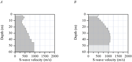
Rayleigh- and Love-wave one-dimensional (1-D) depth-velocity profile correlating with the location along our LA17-4-LCG seismic profile that is nearest to the SCSN LCG strong-motion station. A, Rayleigh-wave 1-D depth-velocity profile showing weak positive gradient in shear-wave velocity (VS) below approximately 12 meters (m) depth. B, Seismic data generated by a 3.5-kilogram sledgehammer and aluminum block source. The Love-wave 1-D depth-velocity profile shows positive gradient in VS between approximately 2 m and approximately 40 m depth. Light grey areas represent regions with few data points. (m/s, meters per second.)
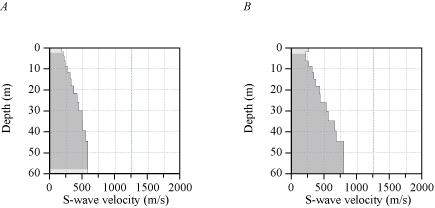
Rayleigh- and Love-wave one-dimensional (1-D) depth-velocity profiles correlating with the location along our LA17-5-RUS seismic profile that is nearest to the SCSN RUS strong-motion station. A, Rayleigh-wave 1-D depth-velocity profile showing weak positive gradient in shear-wave velocity (VS) at all depths. B, Seismic data generated by a 3.5-kilogram sledgehammer and aluminum block source. The Love-wave 1-D depth-velocity profile shows weak positive gradient in VS below approximately 2 m depth. Light grey areas represent regions with few data points. (m/s, meters per second.)
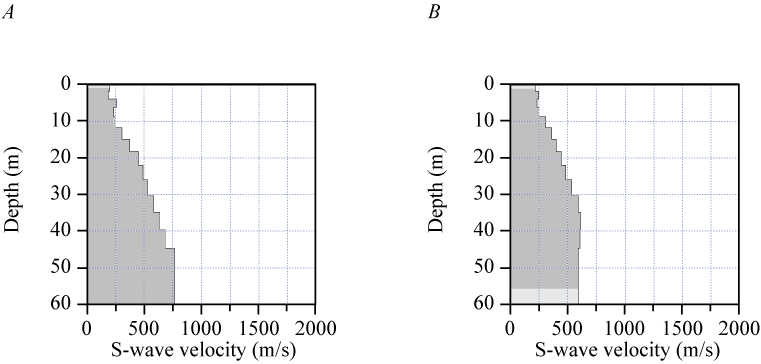
Rayleigh- and Love-wave one-dimensional (1-D) depth-velocity profiles correlating with the location along our LA17-6-STC seismic profile that is nearest to the SCSN STC strong-motion station. A, Rayleigh-wave 1-D depth-velocity profile shows weak positive gradient in shear-wave velocity (VS) below approximately 8 meters (m) depth. B, Seismic data generated by a 3.5-kilogram sledgehammer and aluminum block source. The Love-wave 1-D depth-velocity profile shows weak positive gradient in VS between approximately 2 m and approximately 40 m depth. Light grey areas represent regions with few data points. (m/s, meters per second)
Appendix 4. VP/VS Ratios Determined from P-wave and S-wave Refraction Tomography
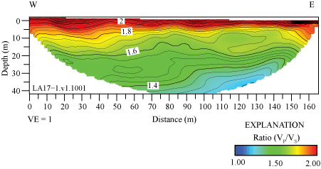
Two-dimensional tomography image of P- to S-wave velocity (VP/VS) ratios along the LA17-1-OLI seismic profile. VP/VS ratios range from about 1.2 to about 2.6 along the seismic profile. (W, west; E, east; m, meters)
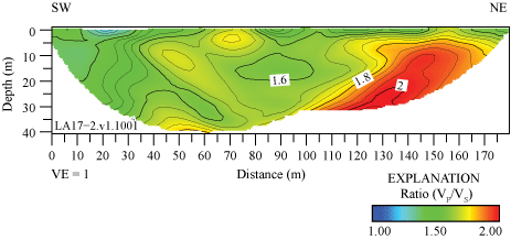
Two-dimensional tomography image of P- to S-wave velocity (VP/VS) ratios along LA17-2-SRN seismic profile. VP/VS ratios range from about 1.2 to about 2 along the seismic profile; the highest (approximately 2) VP/VS ratio coincides with the mapped location of Peralta Hills Fault. (SW, southwest; NE, northeast; m, meters.)
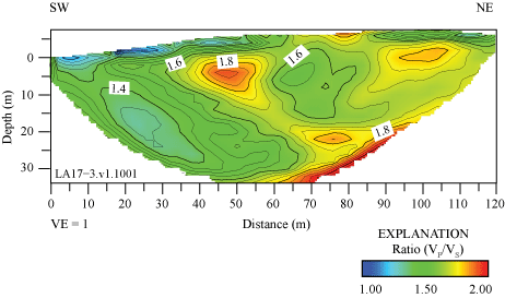
Two-dimensional tomography image of P- to S-wave velocity (VP/VS) ratios along LA17-3-MUR seismic profile. VP/VS ratios range from about 1 to about 2 along the seismic profile. (SW, southwest; NE, northeast; m, meters)
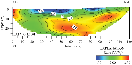
Two-dimensional tomography image of P- to S-wave velocity (VP/VS) ratios along LA17-4-LCG seismic profile. VP/VS ratios range from about 1.4 to about 2.6 along the seismic profile. (SE, southeast; NW, northwest; m, meters.)
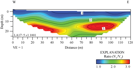
Two-dimensional tomography image of P- to S-wave velocity (VP/VS) ratios along LA17-5-RUS seismic profile. VP/VS ratios range from about 1 to about 3.5 along the seismic profile. (W, west; E, east; m, meters.)
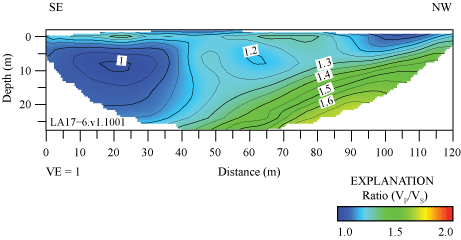
Two-dimensional tomography image of P- to S-wave velocity (VP/VS) ratio along LA17-6-STC seismic profile. VP/VS ratios range from about 1 to about 1.6 along the seismic profile. (SE, southeast; NW, northwest; m, meters.)
Appendix 5. Poisson’s Ratios Determined from P-wave and S-wave Refraction Tomography
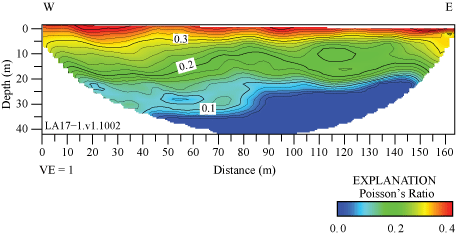
Two-dimensional tomography image of Poisson’s ratios along the LA17-1-OLI seismic profile, derived from P- and S-wave tomography. Poisson’s ratios are highest (approximately 0.4) at the upper approximately 2 meters (m) of the subsurface. (SE, southeast; NW, northwest)
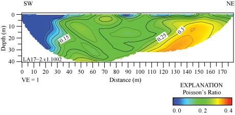
Two-dimensional tomography image of Poisson’s ratios along the LA17-2-SRN seismic profile, derived from P- and S-wave tomography. Highest Poisson’s ratios (approximately 0.3) coincide with the mapped location of Peralta Hills Fault, between approximately 110 and 155 meters (m) distance. (SW, southwest; NE, northeast.)
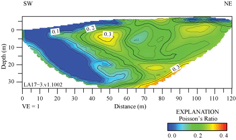
Two-dimensional tomography image of Poisson’s ratios along the LA17-3-MUR seismic profile, derived from P- and S-wave tomography. Poisson’s ratios are highest (approximately 3) at discrete locations across the profile. (SW, southwest; NE, northeast; m, meters)
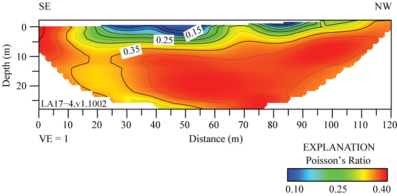
Two-dimensional tomography image of Poisson’s along the LA17-4-LCG seismic profile, derived from P- and S-wave tomography. Poisson’s ratios are highest (approximately 0.35) at depths below approximately 5 meters (m). (SE, southeast; NW, northwest)
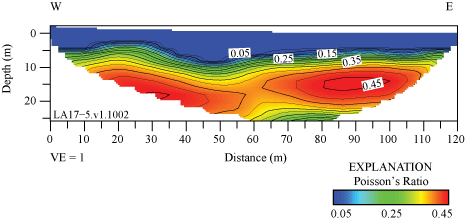
Two-dimensional tomography image of Poisson’s ratios along the LA17-5-RUS seismic profile, derived from P- and S-wave tomography. Poisson’s ratios are highest (approximately 0.4) at depths below approximately 15 meters (m). (W, west; E, east.)
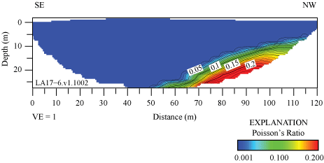
Two-dimensional tomography image of Poisson’s ratios along the LA17-6-STC seismic profile, derived from P- and S-wave tomography. Poisson’s ratios are highest (0.2) at depths below approximately 20 meters (m) in the northwest end of the seismic profile. (SE, southeast; NW, northwest)
Abbreviations
1-D
one-dimensional
2-D
two-dimensional
AWD
accelerated weight-drop
CMPCC
common midpoint cross-correlation
GMPEs
ground-motion prediction equations
Hz
hertz
MASW
multichannel analysis of surface waves
MASLW
MASW using Love-waves
MASRW
MASW using Rayleigh-waves
SCE
Southern California Edison
SCSN
Southern California seismic network
VP
P-wave or compressional-wave velocity
VS
S-wave or shear-wave velocity
VS30
time-averaged shear-wave velocity in the upper 30 meters of the subsurface
Publishing support provided by the Moffett Field Publishing Service Center
Manuscript approved for publication February 22, 2024
Layout and design by Cory Hurd
Disclaimers
Any use of trade, firm, or product names is for descriptive purposes only and does not imply endorsement by the U.S. Government.
Although this information product, for the most part, is in the public domain, it also may contain copyrighted materials as noted in the text. Permission to reproduce copyrighted items must be secured from the copyright owner.
Suggested Citation
Chan, J.H., Catchings, R.D., Goldman, M.R., Criley, C.J., and Sickler, R.R., 2024, Evaluation of 2-D shear-wave velocity models and VS30 at six strong-motion recording stations in southern California using multichannel analysis of surface waves and refraction tomography: U.S. Geological Survey Open-File Report 2024–1016, 58 p., https://doi.org/10.3133/ofr20241016.
ISSN: 2331-1258 (online)
Study Area
| Publication type | Report |
|---|---|
| Publication Subtype | USGS Numbered Series |
| Title | Evaluation of 2-D shear-wave velocity models and VS30at six strong-motion recording stations in southern California using multichannel analysis of surface waves and refraction tomography |
| Series title | Open-File Report |
| Series number | 2024-1016 |
| DOI | 10.3133/ofr20241016 |
| Publication Date | April 18, 2024 |
| Year Published | 2024 |
| Language | English |
| Publisher | U.S. Geological Survey |
| Publisher location | Reston, VA |
| Contributing office(s) | Earthquake Science Center |
| Description | Report: vii, 58 p.; Data Release |
| Country | United States |
| State | California |
| Online Only (Y/N) | Y |