

Airborne Lidar Accuracy Analysis for Dual Photogrammetric and Lidar Sensor Pilot Project in Colorado, 2019
Links
- Document: Report (4.6 MB pdf) , HTML , XML
- Data Release: USGS data release - Hybrid lidar/imagery sensor validation survey data, 2019
- NGMDB Index Page: National Geologic Map Database Index Page (html)
- Download citation as: RIS | Dublin Core
Introduction
This report presents accuracy assessment results of the light detection and ranging (lidar) data collected in Colorado during a pilot project in fall 2019 and supplements the work published in Kim and others (2020). The purpose of the pilot project was to assess the accuracy of lidar and imagery data collected simultaneously for the U.S. Department of Agriculture (USDA) National Agriculture Imagery Program (NAIP) and the U.S. Geological Survey (USGS) National Geospatial Program 3D Elevation Program (3DEP). A multiagency group consisting of U.S. Department of the Interior agencies and USDA agencies participated in the effort. Department of the Interior agencies included Bureau of Land Management (BLM), National Park Service, and USGS; USDA agencies included the Farm Services Agency, the Natural Resource Conservation Service, and U.S. Forest Service (USFS). This pilot project was designed to help determine if a lidar sensor system has the potential to meet future 3DEP topographic lidar collection requirements, ideally at the same altitudes and leaf-on times that NAIP is flown.
The airborne sensor system from Leica Geosystems (part of Hexagon) (hereafter referred to as dual sensor system) was used in the pilot project and can collect imagery and three-dimensional (3D) point cloud data concurrently. This report examines the characteristics of lidar data from a geometric accuracy perspective. Field surveys were performed to evaluate the 3D absolute and relative accuracy of the airborne lidar data and to determine if the data met 3DEP specifications.
Background
3DEP is a partnership program with State, local, and Federal partners that is managed by the USGS to respond to growing needs for high-quality topographic data and for a wide range of other 3D representations of the natural and constructed features in the United States. 3DEP informs critical decisions that are made across the Nation every day, which depend on elevation data ranging from immediate safety of life, property, and the environment to long-term planning for infrastructure projects.
NAIP acquires aerial imagery during the agricultural growing seasons in the continental United States. This “leaf-on” imagery is used as a base layer for geographic information system programs in the Farm Services Agency’s County Service Centers and is used to maintain the Common Land Unit boundaries. Because the airborne lidar sensor system analyzed is a hybrid sensor that collects imagery and lidar data simultaneously, it has the potential to collect data that satisfies USGS 3DEP and USDA NAIP requirements in a single collection.
This report presents accuracy assessment results of the light detection and ranging (lidar) data collected in Colorado during a pilot project in fall 2019 and supplements the work published in Kim and others (2020). The focus of this report is on the geometric quality and characteristics of the lidar data.
Procedures
Procedures used in the pilot project in Colorado in 2019 are described in this section. Procedures included site selection and field campaigns for data collection and procedures for data acquisition. The airborne dual sensor system (lidar and photography) data were collected over two areas with distinct land use patterns (in August–September 2019). In this report, these areas are termed western area of interest (AOI) and eastern AOI. The western AOI included land managed by BLM and USFS near Granby, Colorado. The eastern AOI included agricultural and urban areas in Windsor County, Colo. The two pilot AOIs were selected to be flown in north-central Colorado over two different physical settings to evaluate the system’s performance (fig. 1); therefore, to test the lidar data for geometric accuracy, two distinct surveys were planned and designed (Irwin and others, 2020).
Field data were collected by the USGS in two different field campaigns. The first took place in the western AOI near Granby, Colo., on September 8–11, 2019. The second took place in the eastern AOI east of Fort Collins, Colo. on November 18–20, 2019. The western AOI included six field sites. Four were on land managed by BLM, one site was on land managed by USFS and one was at Windy Gap wildlife area. The eastern AOI included four field sites. The first consisted of two houses in the southeastern part of Fort Collins, Colo. The remaining sites were Chimney Park, Windsor Main Park, and Eastman Park, all within Windsor, Colo. (fig. 2C).
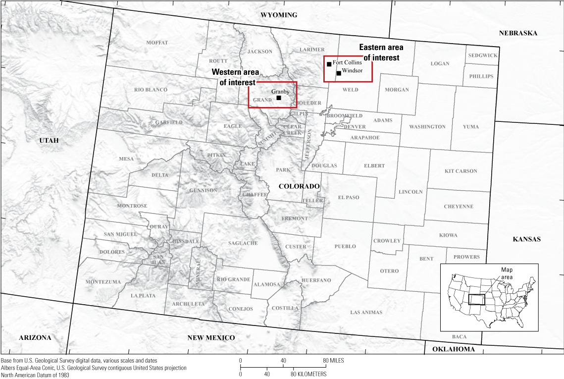
Location of areas of interest (AOI) in Colorado.
Data Acquisition
Hexagon acquired data for this project using the CountryMapper sensor system operating at an altitude of 3.6 kilometers (km), a speed of 180 knots, a pulse repetition frequency of 750 kilohertz (KHz) and a scan rate of 112 Hz. The resulting imagery product was 20 centimeters (cm) ground sample distance ortho imagery and a pulse density of 2.9 points per square meter (ppsm). The elliptical scan pattern of the airborne lidar sensor system allowed for the separation of the point cloud into forward- and backward-looking scanned groups, which enabled intraswath difference analysis.
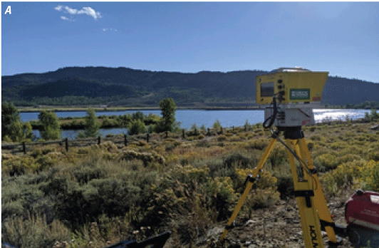
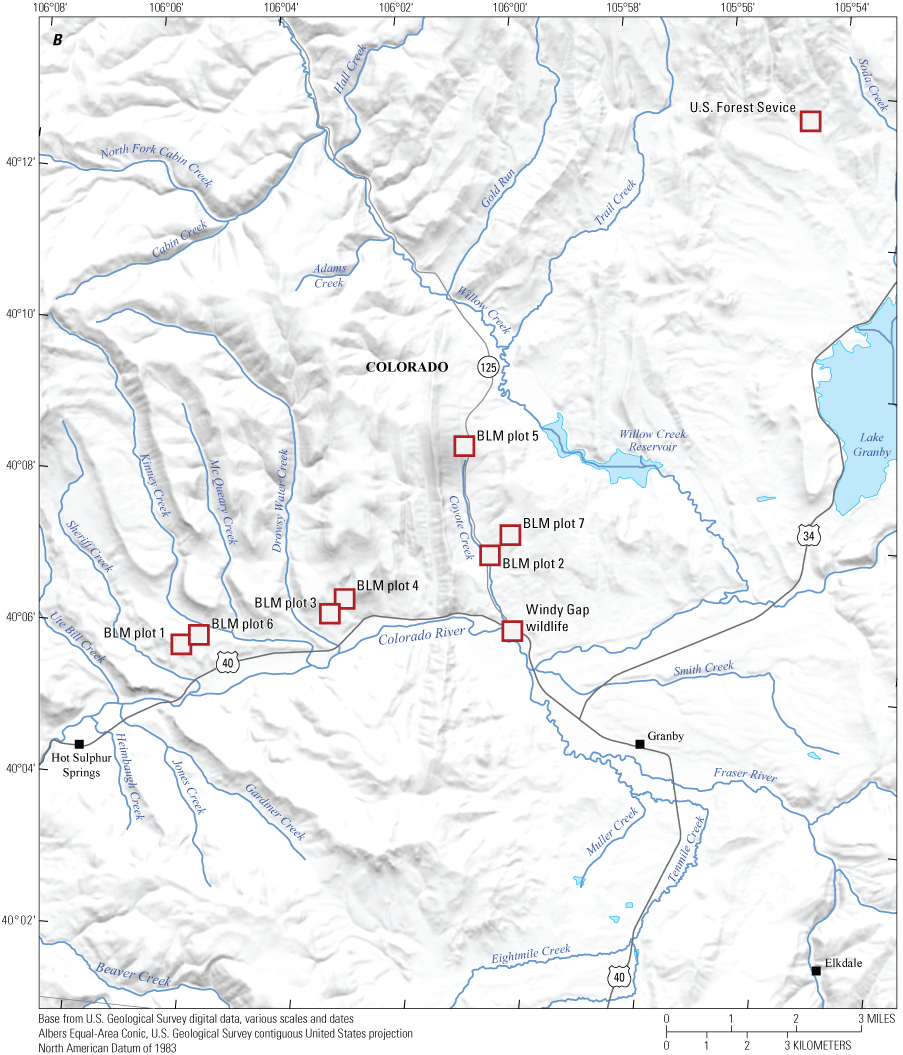
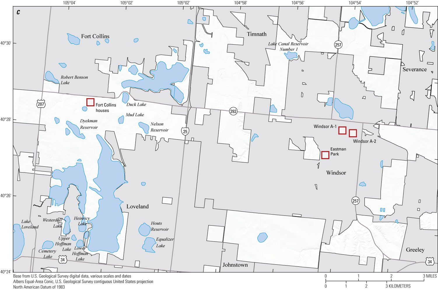
Illustration showing, A, photograph of terrestrial laser scanner used to collect data for the Windy Gap wildlife site in the western area of interest (AOI) site, B, the location of test sites chosen for field visits and detailed surveys using a combination of a terrestrial laser scanner, total station, and global navigation satellite system for data collection of mostly open, vegetated, and forested lands in the western AOI, and, C, the locations of mostly urban sites in the eastern AOI.
Real time kinematic (RTK) global navigational satellite system (GNSS), total station, ground based lidar, unoccupied aerial system (UAS) lidar, and UAS imagery data were collected to compare to the data collected by Hexagon using the airborne lidar sensor system. USGS collected these data using survey-grade GNSS and total station instruments along with a terrestrial laser scanner (TLS). In the RTK method, a fixed base station (base station) occupying either a known location, or a random location that will be post processed to known coordinates, transmits corrections to a moving global positioning system (GPS) receiver (rover). The rover uses these corrections to greatly enhance its positional accuracy, achieving centimeter-level precision (Van Sickle, 2008). The base station data and the rover data were post processed after 16 days, when precise ephemeris of the GNSS satellites were available (Soler and others, 2011). The ground-based lidar is operated by strategically positioning the lidar scanner to ensure full coverage of the target area. These scans from multiple locations are necessary for complete coverage of most targets or those with obstructions. The lidar systematically emits laser pulses and records the return time and intensity of the reflected light, capturing millions of data points. Reflective targets are placed in the region of data collection, and their positions are surveyed using a total station that utilized control established via RTK methods. These targets are used to georeference the lidar data scans and improve the accuracy of merging multiple scans (Bethel and others, 2005). The GNSS and total station data include points collected on ground surfaces, roof planes, infrastructure features, TLS georeferencing spheres, and individual trees. The total station is especially useful in acquiring ground points under tree canopy, where GNSS solutions are difficult to establish. The TLS data include scans of buildings, parking lots, and groups of trees. USGS also collected UAS data. All survey data, including the UAS data, are available at https://doi.org/10.5066/P9CPDWUU (Irwin and others, 2020).
Measurements and Analysis
The analyses quantify the interswath, intraswath (same surface precision), and the absolute geometric errors of airborne lidar data. The quantification (and verification) is important because these errors are indicators of the geometric quality of the data. A dataset can be said to have good geometric quality if (geometric) measurements of identical features, regardless of their position or orientation, yield identical results. Good geometric quality indicates that the data are produced using sensor models that are working as they are mathematically designed and data acquisition processes are not introducing any undue data distortion.
To investigate the quality of the data, USGS assessed absolute and relative (intraswath and interswath) geometric accuracy of the data. The USGS’ Lidar Base Specifications (LBS) version 2.0 defines many quality levels for obtaining lidar data. The airborne lidar data were collected to satisfy the requirements defined by quality level (QL) 2. A detailed description of the quality levels can be obtained from the LBS (National Geospatial Program Standards and Specifications, 2022), and the relevant quality levels for the analysis are listed in table 1.
Table 1.
Lidar data requirements from the Lidar Base Specifications for geometric accuracy of quality level 2 lidar data relevant for this report.[QL2, quality level 2; lidar, light detection and ranging; LBS, Lidar Base Specifications; m2, square meter; ≤, less than or equal to; <, less than; m, meter; RMSE, root mean square error; CE 95, circular error at 95th percentile]
The relative accuracy assessments consisted of two tests: The intraswath or same surface precision of the data and the interswath accuracy, as measured by comparing overlapping regions of a swath (Stensaas and others, 2018). The external or absolute accuracy of the data were measured by testing data against data collected using means of higher accuracy. These included the total station, GNSS, and TLS measurements, and the UAS lidar data. It must be noted that the methods used to quantify (and verify against the USGS lidar base specification) differ from the methods outlined in the LBS. The methods used in this report provide an alternate process to verify the results obtained from the incumbent methods and add quality indicators related to horizontal accuracy that is not tested in the incumbent methods.
Intraswath Analysis and Lidar Density Quantification
The density and the intraswath errors were computed by manually delineating eight polygons (using ArcGIS version 10.8.1 and LP360 software version 2021.1.47.0) in the data. The number of points that fall within the polygon and the area of the polygon are used to compute the density. These polygonal regions were carefully chosen to be as planar as possible (for example, roads known to be smooth, building roofs, parking lots, and so on; fig. 3).
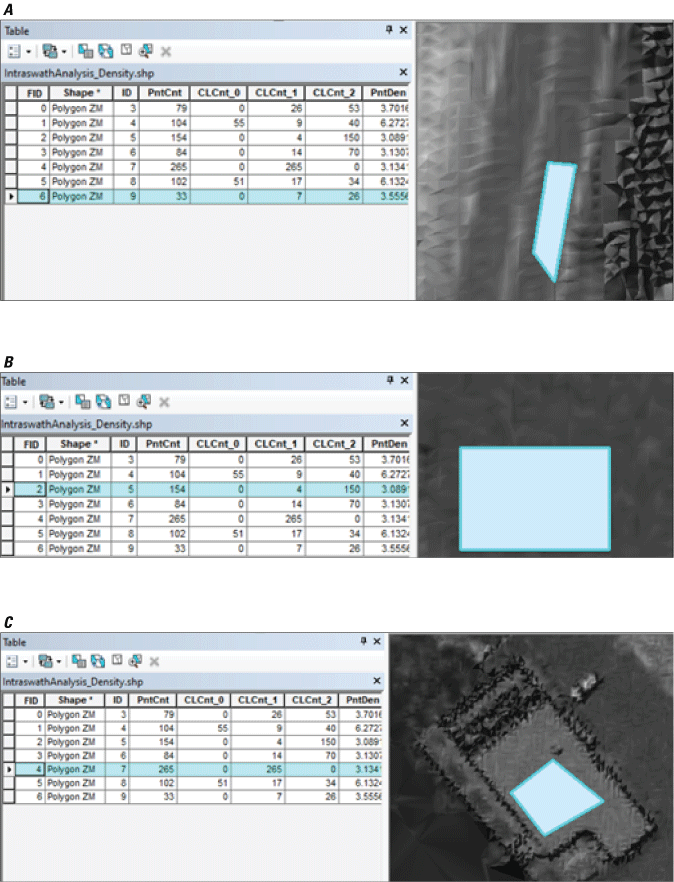
Sample locations used for calculating data density and intraswath precision. A, parts of a smooth road; B, parts of a parking lot; and, C, parts of a roof.
The observed density in the data is shown in figure 4. The regions were selected across the dataset, and the density ranges from 3.1 to 3.7 ppsm, which is better than the requirement for QL2 data as mentioned in table 1 (fig. 4). A couple of regions were chosen in areas of overlapping swaths and where the point density is proportionally (to the number of swaths) higher.
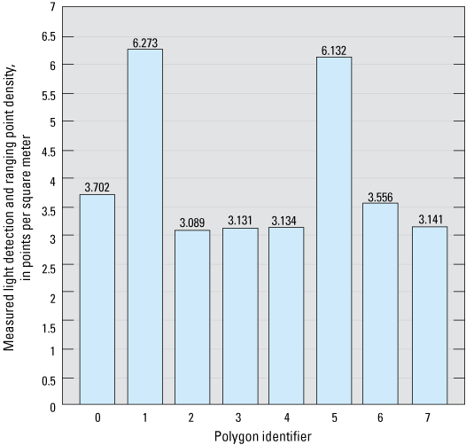
Bar chart showing density estimates from eight polygons.
For intraswath analysis, the precision was measured by fitting a plane through the points inside the manually delineated polygons and then calculating the root mean square error (RMSE) of the planar fit. Generally, the intraswath precision values were very high, better than 1 cm in most cases (fig. 5).
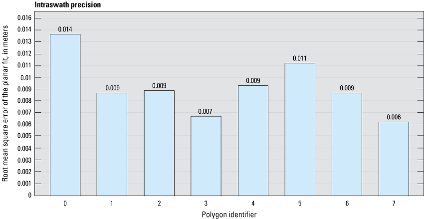
The intraswath precision of lidar data.
Interswath Analysis
Figure 6 shows a profile of a hypothetical surface that falls in the overlapping region of two adjacent swaths. The surface as defined by the swaths is shown in lighter dotted lines, whereas the solid profile represents the actual surface. A poorly calibrated system leads to at least two kinds of errors in lidar data: (1) the same surface is defined in two (slightly) different ways (relative or internal error) by different swaths, and (2) the deviation from actual surface (absolute error). The calibration procedures are of less concern than the final quality of data; however, a process to test the quality of instrument calibration is needed, because a well-calibrated instrument is a necessary condition for high-quality data. Therefore, the interswath error (along with the intraswath error) is an important direct measure of the quality of instrument calibration.
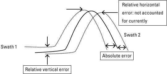
Surface uncertainties in hypothetical adjacent swaths (adapted from Stensaas and others, 2018).
The interswath analysis was done by using the American Society for Photogrammetry and Remote Sensing (ASPRS) Data Quality Metrics (DQM; Stensaas and others, 2018) tool to analyze the swath-to-swath overlapping regions. In this method, data in each tile is split into their component swaths. The ASPRS DQM method implements the concept of point-to-plane data quality measures over natural surfaces. The prototype works on ASPRS’s LASER file exchange format (LAS) files containing swath data. If the swaths are termed Swath 1 and Swath 2 (fig. 7), the software uniformly samples single return points in Swath 1 and then chooses “n” (user input) points. The neighbors of these “n” points (single return points) in Swath 2 are determined.
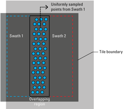
Interswath analysis on a per tile basis. Diagram shows that the1,000 points per swath overlap are uniformly chosen for analysis (adapted from Stensaas and others, 2018).
A least squares plane is fit through the neighboring points using eigenvalue/eigenvector analysis in a manner like principal component analysis. The equation of the planes is the same as the component corresponding to the least of the principal components. The eigenvalue/eigenvector analysis provides the planar equations as well as the RMSE of the plane fit. The use of single return points in conjunction with a low threshold for RMSE is used to eliminate sample measurements from nonhard surfaces (such as trees). The DQM software calculates the offset of the point (say “p”) in Swath 1 to the least squares plane. The output includes the offset distance as well as the slope and aspect of the surface as implied in the planar parameters.
The software was used to calculate the interswath differences on a per tile basis in the western AOI and the eastern AOI. The results are graphically shown in figure 8 and summarized in table 2. A total of 780 tiles of lidar data in the western AOI and 188 tiles of lidar data in the eastern AOI were tested for this analysis.
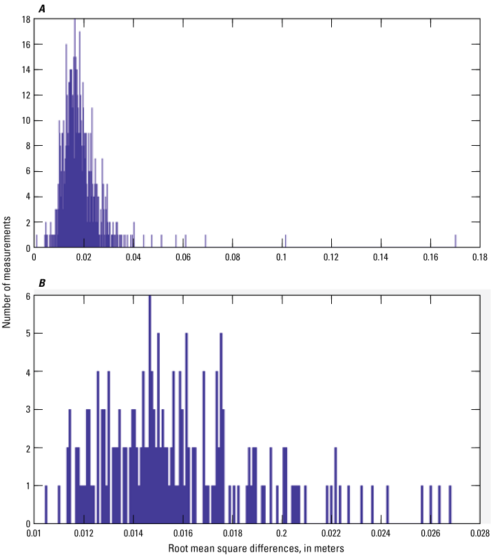
Histogram plot of root mean square differences in the, A, western area of interest, which is predominantly rural, ranches, and forest areas, and, B, the eastern area of interest, which is predominantly urban areas.
Table 2.
Summary of interswath measurements across 780 tiles in the western area of interest and 188 tiles in the eastern area of interest.[AOI, area of interest; RMSD, root mean square difference; m, meter]
In most tiles (99 percent), the root mean square difference values measured were 0.04 m or less for the western AOI and 0.026 cm or less for the eastern AOI. These values are well within the QL2 requirements of the LBS as stated in table 1 and, together with the analysis in the previous section (and figs. 2 and 3), indicate that the data are well calibrated.
Absolute Geometric Accuracy Assessment
The absolute accuracy of airborne lidar data is divided into quantitative and semiquantitative sections. The measurements shown in semiquantitative sections (such as comparison of tree heights and comparison of locations of lane markings) have subjective components to them; however, we consider them to be important metrics towards understanding of the accuracy of the data.
Semiquantitative Measurements and Analysis: Tree Heights
The assessment survey involved collecting total station data as well as TLS data for trees to compare the tree heights obtained from total station and TLS to the airborne data. A UAS-based lidar sensor was also flown to collect lidar data that were compared to the airborne lidar data (fig. 9).
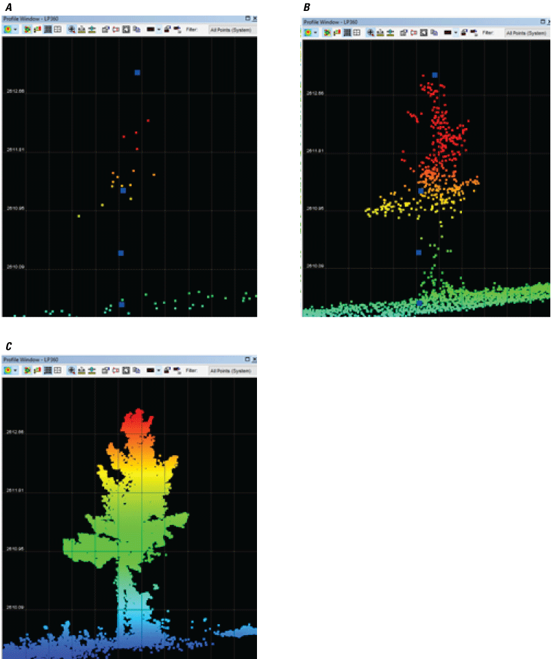
Measurements on trees. Profile of total station points (in blue) laid along with, A, airborne lidar data; B, uncrewed airborne system lidar data; and, C, terrestrial laser scanning lidar data.
Individual trees were selected in the field, and total station points were collected along its trunk up to the highest observed leaf or branch. It is acknowledged that the ability of the total station (and TLS) to accurately obtain tree heights is dependent on the location of total station (or TLS) instrument as well as obstructions; therefore, care was taken to select the instrument locations such that the best view of the selected trees was available in areas of high-density trees. It may not be possible to collect data on the top of trees using a TLS or total station if the line of site is obstructed (fig. 10).
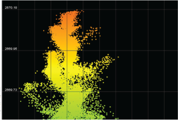
Profile of a coniferous tree scanned using terrestrial laser scanning. The treetop appears to be missing or cut off because of interference from branches of other trees.
Three elevation measurements for each tree were noted: the highest elevation from the total station measurements, the highest elevation from the TLS points, and the highest elevation point of the airborne lidar sensor system. The differences among the airborne lidar data and measurements from the total station as well as TLS were noted. When compared to the elevation of trees obtained from total station data, the airborne lidar data generally were lower by 0.33 to 1.25 m in the BLM plots (table 3). This result has been documented in Andersen and others, 2006. Other studies have determined that the consistency between tree heights is higher if the systems are optimized for capturing vegetation as opposed to bare earth (Wang and others, 2019). The difference between total station- and TLS-based measurements is high in the USFS plot for two possible reasons: (1) the higher density of trees (in USFS plots as compared to BLM plots) can make it difficult for total station-based measurements to capture the top of trees, and (2) the TLS measurements were made from multiple stations, which can increase the chances of capturing top of trees.
Quantitative Measurements and Analysis: Vertical Accuracy and 3D Accuracy
Assessing absolute accuracy in rural areas with few well-defined features that can provide reliable horizontal coordinate measurements is difficult and this assessment is therefore limited to only a vertical accuracy assessment. In this survey, check points were surveyed in clear and open areas as well as in vegetated areas such as in tall grass and shrubs and below tree canopy. The vertical accuracy measurements presented here are measured against only those points classified as ground in the final airborne lidar data. The LP360 software as well as the DQM software were used to derive the measurements. The results presented here are from the LP360, although the DQM software measurements were comparable. Figure 11 shows examples from two locations in the western AOI.
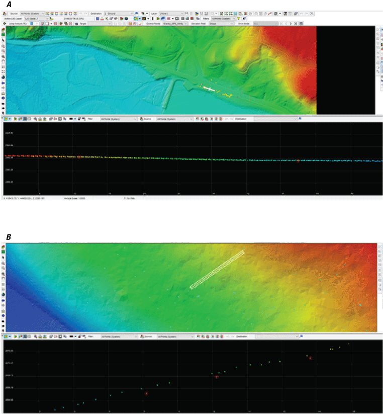
Profile of check points (“+”’dots) against the airborne lidar profile in, A, Windy Gap wildlife area and, B, U.S. Forest Service plot.
Table 4 lists the summary of measurements from western AOI survey locations. Only the Windy Gap wildlife area measurements can be considered ideal for nonvegetated vertical accuracy assessment because those were made over concrete or asphalt surfaces in clear and open areas. Most other locations had substantial cover of shrubs or trees (in the case of USFS plot). The measurements indicate the airborne lidar data are within the specifications for QL2. Table 5 lists the vertical measurements of site surveyed in the eastern AOI. The RMSE ranges from 0.028 to 0.035 m. Tables 4 and 5 indicate that in clear and open areas, the airborne lidar data are well within the requirements specified in the LBS (less than 0.10 m RMSE from table 1) for open areas as well as in vegetated areas. The USFS locations were not considered clear and open as they had substantial tree cover.
Table 4.
Vertical accuracy measurements in the western area of interest.[AOI, area of interest; m, meter; RMSE, root mean square error; USFS, U.S. Forest Service; BLM, Bureau of Land Management].
Horizontal Accuracy Assessment
The horizontal component of accuracy for 3DEP lidar data is not explicitly verified in most 3DEP projects collected under Geospatial Products and Services Contracts. The LBS does not provide quality thresholds or methods for verification of data; therefore, the methods presented in this section are forward-looking research efforts to develop operational methods for verifying 3D accuracy (horizontal and vertical) in future versions of the LBS.
In this report, we present three methods to verify the horizontal component of the airborne lidar data accuracy:
-
· Scanning roof planes of houses and other structures using a TLS system and comparing data with airborne lidar data
-
· Collecting roof plane measurements using total station and comparing data with airborne lidar data
-
· Comparing point measurements of traffic and parking lot markings on freshly paved road surface to their image in airborne lidar intensity images (fig. 12).
The three-dimensional image from the TLS scan is colorized using the red, green, and blue values obtained from the camera collocated with the TLS. This TLS method used manual building roof extraction and comparison of plane intersections using methods described in Kim and others (2020). The total station method used automatic estimation of shift in data (between reference total station and airborne lidar) using methods described in Stensaas and others (2018). The background image for the lidar intensity method was derived from the airborne lidar’s intensity data collected over a parking lot.
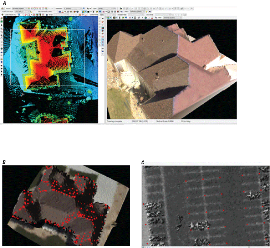
Examples of absolute accuracy assessment methods used on the airborne lidar data (three-dimensional accuracy). A, building roof planes scanned using terrestrial laser scanning. B, total station-based points collected on a building roof surface. C, check points collected on visible parking lot or road markings on freshly paved and painted surfaces.
Terrestrial Laser Scanner Method
The first method, which is described in Kim and others (2019), uses TLS lidar data from preselected building roof planes. The roof planes were manually delineated and mathematically modeled. The intersection points of these roof planes were calculated. The same process (of manually extracting and mathematically modeling the roof planes) was repeated on conjugate roof planes from the airborne lidar data, and the intersection points of the various roof facets were calculated. The 3D accuracy of the points was assessed by comparing the two sets of coordinates. This process was repeated for multiple buildings across the eastern AOI. A detailed report of the procedures, mathematical modeling, and analysis is in Kim and others (2020).
The results from the analysis indicate that the airborne lidar is translated by 0.22 m (standard deviation [s.d.]: 0.033 m) in easting, 0.074 m (s.d.: 0.096 m) in northing and 0.034 m (s.d.: 0.016 m) in elevation (Kim and others, 2020).
Total Station Method
The second method explored was using total station points obtained by carefully pointing the total station viewer to the planes of roofs and measuring points (coordinates) on the surface in reflectorless mode. These points are considered reference check points. This method explores an automated solution to determine the discrepancy in geometric positioning between reference data and airborne lidar data. In figure 13, the check points measured by the total station are notionally illustrated as red dots, and the airborne lidar points illustrated on roof planes are in blue. A two-dimensional neighborhood of points is selected around the total station check point. Since these points are carefully curated during data collection, there is high confidence that the two-dimensional neighborhood of points lie on the roof plane. The equation of the plane is determined by fitting a plane to this neighborhood of points, and the distance of the plane from the check points are calculated. This process is repeated for all the check points collected. The method assumes that the geometric discrepancy between the airborne lidar and the total station points, at the scale of a building or small neighborhood, can be estimated by a single shift (∆; for example, ∆X, ∆Y, ∆Z). The step-by-step process is below:
-
• Use curated total station collected points to develop and model individual roof plane equations.
-
– [P]i_TS=[a, b, c, d]i, i=1,2,.. number of planes>3 in at least three directions. The planes equation used is straightforward: [aX+bY+cZ=d]i. Here, P represents individual planes, and [a, b, c, d] represent the planar parameters and [X,Y,Z]i represents the coordinates of the total station points belonging to plane i.
-
-
• Gather aerial lidar points (from dataset to be evaluated) for each plane. Points can be gathered by manual or automatic means. In this case, we used neighborhood queries using spatial indexing structures to collect points in the aerial lidar point cloud that are closest to the total station collected points. The data structures are built into the ASPRS DQM software.
-
• Fit aerial lidar to (total station check point derived) plane equations and optimize.
-
– Minimize ∑|Pi_TS(Xi_lidar+e)| to determine e=(ex, ey, ez). The e is the estimated displacement between the lidar data and the model of the building roof planes derived from total station points. This displacement is considered as the estimate of error in the lidar data. The Xi_lidar represents individual lidar points (from airborne lidar) that belongs to plane Pi_TS.
-
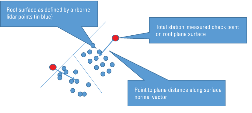
Notional representation of check points collected using total station (red) and the neighboring airborne lidar points over a building (in blue). The normal vectors of the building’s plane are estimated from the neighborhood of points (that is, for each point, an estimate of the mathematical equation of the underlying plane is derived).
Table 6 contains the results of four sites using this method, and appendix 1 table 1.1 shows the measurements in more detail. The measurements shift is estimated by taking the pseudo inverse of the matrix formed by the columns (Nx, Ny, Nz, which represent the equations of the plane) and multiplying it with the corresponding point-to-plane distance vector column.
Table 6.
Horizontal accuracy estimates using total station measurements on building roof surfaces.[∆, axis shift; m, meter]
The average 3D shift between the airborne lidar data and the total station data were determined to be (0.19 m, 0.078 m, 0.057 m) with this method. Two measurements involved roof planes from multiple houses or structures.
Lidar Intensity Method
The third method (fig. 14) for observing horizontal errors in the data involved using check points collected on visible parking lot or road markings on freshly paved surfaces. This method is the most common method used in the industry (when possible) and is analogous to the data quality assessment methods used for aerial and satellite imagery. Because the LBS do not require horizontal accuracy to be reported with the 3DEP data delivery, these measurements are usually made by the data vendors for their internal processes and not externally reported.
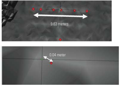
Comparison of check points in intensity data (the image on the right is a zoomed in view of the measurements shown in left). The red dots are the measured check points, and the green dot is the corresponding point in airborne lidar data (delineated manually).
The airborne lidar intensity data were used to identify parking lot line intersections. These check points were selected before the survey in the intensity airborne lidar data, and GNSS (real-time kinematic) methods were used to measure the same check points. The measured differences were noted in only one parking lot and were on an average (0.15 m, 0.06 m, and 0.04 m) in easting, northing, and elevation, respectively. The lower density of QL2 (2 ppsm) precludes a precise location of such intersections. They also require manual delineation; however, with increasing point density (QL1 and QL0 or higher), such methods could offer the least expensive mode of precision testing the 3D accuracy of data, and established image processing toolsets may be able to extract more precise locations of such check points from denser lidar datasets.
Operational Considerations for Assessment of Lidar Data
The objectives of this exercise include examining ways to operationalize the task of quantifying the geometric characteristics of 3DEP lidar data, identifying opportunities for automation, identifying tasks that are bottlenecks (in terms of time), and highlighting methods that can be used for streamlining the process. Table 7 lists and categorizes all the important tasks involved in developing this data quality assessment report. Most of the tasks are listed chronologically. The data acquisition is considered outside the scope of this processing flow.
Table 7.
List of all tasks required for geometric data quality assessments presented in this report.The absolute accuracy assessment is dependent on inputs from the survey, whereas all other aspects of the assessment can be done without field survey. The actual survey (Irwin and others, 2020) consists of several steps (base station setup, instrument locations, tie point target locations, data collection, and so on) and is physically demanding as well as time consuming. Depending on the location of the surveys, these are also difficult in terms of rework. The fact that the field survey is the most time consuming and perhaps expensive part of the tasks (ignoring the data acquisition and focusing only on data validation parts), the objectives and key results obtainable along with the requirements of key stakeholders warrant careful consideration; furthermore, the complexity in terms of coordination and preparation increases if field surveys and lidar data acquisition are simultaneous. In most cases, surveys could be done after lidar acquisition, which reduces complexities arising out of coordination and allows the surveyor to choose targets that are optimal for assessing the dataset in question.
The table shown in appendix 1 table 1.1 lists the estimate time required to collect and process the data for each of the sites visited in this work. Of note, travel, site selection, and site access times have not been included. Operating and collecting the requisite data using the laser scanner, as well as the GNSS base station data collection (at least 2 hours of occupation), clearly contributes to a substantial amount of time; therefore, any future optimization efforts to reduce time required for data collection and processing may benefit from focusing on reducing time required for performing these two tasks. Existing base stations operated by external agencies in the vicinity could be part of the solution, such as a Real Time Network (RTN) service; however, it should be noted that not all RTNs operate in the National Spatial Reference System and RTN services require cell service with mobile internet connections for positional corrections and therefore may not be available in remote areas such as BLM- and USFS-managed lands. Faster laser scanners could also substantially reduce the time required for laser data collection and processing. These scanners allow more set ups in less time, which increases the coverage of data. With the latest scanners, the limiting step (in terms of time) becomes the GNSS base station collection time (which is currently 2 hours); therefore, if 20 well-distributed 3D targets are to be examined, a total of at least 40 hours would be required for just collecting data (20 check points are the minimum required for reporting the quality of geospatial data [ASPRS geospatial data accuracy standards; ASPRS Map Accuracy Standards Working Group, 2015). Here, we assume that the same GNSS station cannot be used between two targets; however, it should also be noted that a GNSS rover can operate within a 10-km radius of its GNSS base station and still get solutions that are survey grade, potentially making it possible to collect numerous well-distributed 3D targets from one base station setup.
Comparative Discussions of the Methods
The three methods mentioned here (using TLS, total station, and GNSS measurements over visible targets) each have their advantages and disadvantages as described below:
Time required for data collection and processing: All three methods depend on setting up a base station (over a National Geodetic Survey-published control point) or collecting GNSS data over a point established for the survey for at least 2 hours. The TLS methods also take more time to acquire and process data.
Equipment availability: The equipment (laser scanner) is expensive and may not be available with licensed surveyors (as compared to a total station and GNSS receivers);
Visualization and ease of understanding data: The TLS data provide more context and are easy to visualize if an appropriate software is available (for example, LP360, CloudCompare). Total station points can be visualized in most geographic information system software (for example, Esri, Global Mapper, GRASS).
Accuracy: The individual total station points are probably at least as precise, if not more, than the individual TLS points. However, the TLS points over planar features of interest can be numerous (in the thousands) compared to the numbers of TS points (typically in tens of points). Theoretically, the availability of thousands of points can make the parameters describing the planar features more robust; however, in terms of final accuracy of the results, more study would be beneficial.
Summary
The U.S. Geological Survey (USGS) analyses of the airborne lidar data collected for a pilot project in Colorado in 2019 show these data appear to satisfy the USGS quality level 2 requirements. The fact that the methods used to verify the data are different from the methods that industry uses indicates the robustness of the conclusions. The report also demonstrates that the practice of assessing the three-dimensional (3D) absolute accuracy of lidar point clouds is useful in assessing the quality of data. The USGS Earth Resources Observation and Science Center plans to continue to work on improving ground survey protocols. Despite some limitations (such as temporal separation between airborne lidar data collection and ground survey data collection), the report demonstrates that the methods for assessing the geometric accuracy of data can be effective for large scale projects.
Of note, the pilot project was flown at lower altitudes to support 20-centimeter Ground Sample Distance National Agriculture Imagery Program imagery collection, so no assessment can be made about meeting 3D Elevation Program requirements from altitudes needed to collect 1-meter imagery for entire states. Also, in terms of ability to collect data leaf-on, although this pilot project demonstrated that ability, the areas included in the pilot project in northern Colorado are sparse in terms of vegetation cover, especially deciduous trees. Conducting a pilot project in the future at higher altitudes over much denser vegetation would be provide a more nuanced assessment of the benefits, and aid decision making process.
This report’s investigations on the methodologies used for data assessments and their relative advantages and disadvantages are important for operationalizing the absolute accuracy assessment process. The report also is indicative of the efforts required to characterize a sensor system to ensure that these sensors can deliver high-quality lidar data to support the 3D Elevation Program.
References Cited
Andersen, H.-E., Reutebuch, S.E., and McGaughey, R.J., 2006, A rigorous assessment of tree height measurements obtained using airborne lidar and conventional field methods: Canadian Journal of Remote Sensing, v. 32, no. 5, p. 355–366. [Also available at https://doi.org/10.5589/m06-030.]
ASPRS Map Accuracy Standards Working Group, 2015, ASPRS positional accuracy standards for digital geospatial data: Photogrammetric Engineering & Remote Sensing, v. 81, no. 3, p. A1–A26, at https://doi.org/10.14358/PERS.81.3.A1-A26.
Bethel, J.S., Johnson, S.D., Prezzi, M., Van Gelder, B.H.W., McCullouch, B.G., Cetin, A.F., Han, S., Hawarey, M, Lee, C., Sampath, A., and Shan, J., 2005, Modern technologies for design data collection: Publication FHWA/IN/JTRP-2003/13, Joint Transportation Research Program, Indiana Department of Transportation and Purdue University, West Lafayette, Indiana. [Also available at https://doi.org/10.5703/1288284313273.]
Irwin, J.R., Sampath, A., Kim, M., Bauer, M.A., Burgess, M.A., Park, S., and Danielson, J.J., 2020, Hybrid lidar/imagery sensor validation survey data, 2019: U.S. Geological Survey data release, accessed April 24, 2023, at https://doi.org/10.5066/P9CPDWUU.
Kim, M., Park, S., Danielson, J., Irwin, J., Stensaas, G., Stoker, J., and Nimetz, J., 2019, General external uncertainty models of three-plane intersection point for 3d absolute accuracy assessment of lidar point cloud: Remote Sensing, v. 11, no. 23, 18 p. [Also available at https://doi.org/10.3390/rs11232737.]
National Geospatial Program Standards and Specifications, 2022, Lidar base specification 2022 rev. A: U.S. Geological Survey, 45 p., accessed April 29, 2024, at https://www.usgs.gov/media/files/lidar-base-specification-2022-rev-a.
Soler, T., Weston, N.D., and Foote, R.H., 2011, The “Online Positioning User Service” Suite” (OPUS-S, OPUS-RS, OPUS-DB): CORS and OPUS for Engineers: Tools for Surveying and Mapping Applications, p. 17–26. [Also available at https://doi.org/10.1061/9780784411643.ch03.]
Stensaas, G., Sampath, A., and Heidemann, K., and the ASPRS Lidar Cal/Val Working Group, 2018, ASPRS guidelines on geometric inter-swath accuracy and quality of lidar data: Photogrammetric Engineering and Remote Sensing, v. 84, no. 3, p. 117–128. [Also available at https://doi.org/10.14358/PERS.84.3.117.]
Van Sickle, J., 2008, GPS for land surveyors (3d ed.): CRC Press, 360 p. [Also available at https://doi.org/10.4324/9780203305225.]
Wang, Y., Lehtomäki, M., Liang, X., Pyörälä, J., Kukko, A., Jaakkola, A., Liu, J., Feng, Z., Chen, R., and Hyyppä, J., 2019, Is field-measured tree height as reliable as believed—A comparison study of tree height estimates from field measurement, airborne laser scanning and terrestrial laser scanning in a boreal forest: ISPRS Journal of Photogrammetry and Remote Sensing, v. 147, p. 132–145. [Also available at https://doi.org/10.1016/j.isprsjprs.2018.11.008.]
Appendix 1. Supplementary Data Table
Table 1.1.
Approximate data collection times and data counts for various tasks.[BLM, Bureau of Land Management; USFS, U.S. Forest Service; GNSS, global navigation satellite system; TLS, Terrestrial Laser Scanner; UAS, unoccupied aerial system]
Abbreviations
3D
three-dimensional
3DEP
3D Elevation Program
AOI
area of interest
ASPRS
American Society for Photogrammetry and Remote Sensing
BLM
Bureau of Land Management
DQM
data quality metrics
GNSS
global navigation satellite system
LBS
Lidar Base Specifications
lidar
light detection and ranging
NAIP
National Agriculture Imagery Program
ppsm
points per square meter
QL
quality level
RMSE
root mean square error
RTK
real time kinematic
RTN
real time network
s.d.
standard deviation
TLS
terrestrial laser scanning
UAS
uncrewed aerial system
USDA
U.S. Department of Agriculture
USFS
U.S. Forest Service
USGS
U.S. Geological Survey
For more information about this publication, contact:
Director, USGS Earth Resources Observation and Science Center
47914 252nd Street
Sioux Falls, SD 57198
605–594–6151
For additional information, visit: https://www.usgs.gov/centers/eros
Publishing support provided by the Rolla Publishing Service Center and Sacramento Publishing Service Center
Disclaimers
Any use of trade, firm, or product names is for descriptive purposes only and does not imply endorsement by the U.S. Government.
Although this information product, for the most part, is in the public domain, it also may contain copyrighted materials as noted in the text. Permission to reproduce copyrighted items must be secured from the copyright owner.
Suggested Citation
Sampath, A., Irwin, J., and Kim, M., 2024, Airborne lidar accuracy analysis for dual photogrammetric and lidar sensor pilot project in Colorado, 2019: U.S. Geological Survey Open-File Report 2024–1036, 22 p., https://doi.org/10.3133/ofr20241036.
ISSN: 2331-1258 (online)
Study Area
| Publication type | Report |
|---|---|
| Publication Subtype | USGS Numbered Series |
| Title | Airborne lidar accuracy analysis for dual photogrammetric and lidar sensor pilot project in Colorado, 2019 |
| Series title | Open-File Report |
| Series number | 2024-1036 |
| DOI | 10.3133/ofr20241036 |
| Publication Date | August 20, 2024 |
| Year Published | 2024 |
| Language | English |
| Publisher | U.S. Geological Survey |
| Publisher location | Reston, VA |
| Contributing office(s) | Earth Resources Observation and Science (EROS) Center |
| Description | Report: v, 22 p.; Data Release |
| Country | United States |
| State | Colorado |