

Using the Horizontal-to-Vertical Spectral Ratio Method to Estimate Thickness of the Barry Arm Landslide, Prince William Sound, Alaska
Links
- Document: Report (12.0 MB pdf) , HTML , XML
- NGMDB Index Page: National Geologic Map Database Index Page (html)
- Download citation as: RIS | Dublin Core
Acknowledgments
We appreciate the forethought and persistence of Michael West and the Alaska Earthquake Center, without whom the installation of seismic stations BAW, BAE, and BAT would not have happened. Multiple agencies collaborated to support work that contributed to this project, including the U.S. Department of Agriculture Forest Service, National Tsunami Warning Center, and Alaska Department of Geological and Geophysical Surveys. The facilities of EarthScope Consortium were used for access to waveforms and related metadata used in this study. These services are funded through the National Science Foundation’s Seismological Facility for the Advancement of Geoscience (SAGE) Award under Cooperative Agreement EAR-1724509. Marc Wathelet of Institut des Sciences de la Terre, Centre National de la Recherche Scientifique, and Institut de Recherche pour le Développement provided invaluable guidance on the inner workings of Geopsy.
The authors are grateful to Lauren Schaefer, Katy Barnhart, and Sean LaHusen of the U.S. Geological Survey for sharing data on landslide event history, previous modeled failure surface depth estimates, and geologic structure at Barry Arm. Alan Yong and Bill Stephenson of the U.S. Geological Survey generously offered their expertise for questions about seismic methods.
Abstract
Conducting detailed investigations of large landslides is difficult, especially in the subsurface, largely due to environmental factors such as steep slopes, difficult access, and numerous objective hazards. These factors have made it challenging to accurately estimate the depth to the failure surface of the Barry Arm landslide, a large (roughly 108 cubic meters), deep-seated bedrock landslide in Prince William Sound, Alaska, recognized in 2019. The landslide has exhibited accelerated movement in recent years and poses a potential tsunamigenic hazard if rapid failure occurs. Failure surface depth, equivalent to landslide thickness, is a necessary metric for landslide-volume calculations and associated tsunami wave models. In this report, we used seismic noise recorded by a seismometer located on the Barry Arm landslide in Alaska to calculate the horizontal-to-vertical spectral ratio (HVSR) to investigate the site fundamental frequency (f0) and depth of the failure surface. To ensure that observed peak frequencies in the spectral ratio were related to the underlying stratigraphy (and not caused by other noise sources like nearby glaciers, topographic resonance, weather, or human activities), we also calculated HVSRs using earthquake signals, HVSRs at other seismic stations within a 2.5-kilometer radius, and a standard spectral ratio between the landslide station and other sites. We observed multiple peaks in the landslide HVSR curves at 1.5 hertz (Hz), 4–5 Hz, and 7–11 Hz. The frequencies of these peaks were consistent at the landslide site through time and across methods and were dissimilar to those identified at other seismic stations in the area, making it unlikely the peaks were caused by local noise.
Directional HVSRs calculated at 15-degree intervals showed amplification of the higher frequency peaks in the direction parallel to slip, indicating two-dimensional site effects. We used the distinct frequency peaks in the seismic record to develop a 4-layer conceptual model of the landslide wherein the top of the deepest layer represents the primary failure surface, or the boundary between damaged (mobile) and undamaged material. We inverted Rayleigh wave ellipticity curves within this 4-layer configuration with constraints on S-wave velocity and layer thickness based on analogous material properties identified in the literature. This was necessary absent any site-specific subsurface S-wave velocity data. The best-fitting models indicate a mean slope-normal depth to the failure surface of 188 (±9) meters (m), with additional stratigraphic boundaries at 4 and 20 m below ground surface, potentially representing layered motion. These results agree with and improve upon ranges estimated by previous studies and can support future modeling and assessment efforts at Barry Arm.
Introduction
In the spring of 2019, a large, slow-moving, and potentially tsunamigenic landslide was recognized at Barry Arm fjord in western Prince William Sound approximately 50 kilometers (km) northeast of Whittier, Alaska (Dai and others, 2020; fig. 1A). Since this initial documentation of deformation history, further analysis of satellite data and historical imagery has revealed episodes of movement dating back at least to the middle of the 20th century, with more rapid movement occurring in the last two decades (Dai and others, 2020; Schaefer and others, 2020, 2022, 2023). The acceleration is temporally coincident with the rapid retreat of the Barry Glacier from 2009 to 2017 (Dai and others, 2020). The landslide has an aerial extent of approximately 3.4 square kilometers (Schaefer and others, 2023) and an estimated volume between 290 × 106 and 689 × 106 cubic meters (m3) (Barnhart and others, 2021). If the slope were to fail catastrophically, it would generate a tsunami that could affect high-use waterways and onshore locations and disrupt the critical harbor infrastructure in Whittier, Alaska (Barnhart and others, 2021).
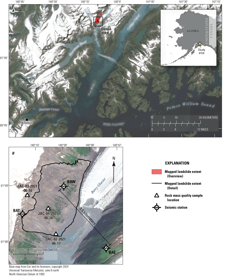
A, Map showing an overview of the Barry Arm landslide site in western Prince William Sound, Alaska, with local place and geographic feature names. The distance from the landslide to Whittier, in the bottom-left corner, is approximately 50 kilometers. Line A–A' illustrates the base width, 7.3 kilometers, used in the topographic resonance calculation. B, Detailed map showing the landslide with the locations of the three seismometers and three rock mass quality sites referenced in this study.
A thorough characterization of the hazard and risk associated with the Barry Arm landslide requires assessment of landslide volume and potential failure mechanisms, both of which are dependent upon accurate estimates of landslide depth and failure surface geometry. Preliminary hazard models and volume estimates at the site have relied on expressions of the headscarp(s) and simplifying assumptions about the subsurface slide geometry, resulting in a high degree of uncertainty (Barnhart and others, 2021). Although direct methods for characterizing landslide depth are impractical for this landslide given the objective hazards and local environmental regulations, geophysical methods can yield valuable information related to the structure of the subsurface. Passive recordings of the ambient seismic wavefield have been used in previous studies to determine landslide thickness and probe the subsurface structure (for example, Pazzi and others, 2017; Thomas and others, 2020; Calamita and others, 2023).
The horizontal-to-vertical spectral ratio (HVSR) of the Fourier spectra of horizontal and vertical components of seismic noise (Nakamura, 1989) is a common method to estimate thickness of unconsolidated sediments over bedrock in basins (for example, Gosar, 2017; Martorana and others, 2018; Panzera and others, 2019). This method requires only a single seismometer and a limited recording time (on the order of minutes to hours). The HVSR—or derivative analyses like the Rayleigh wave ellipticity curve (for example, Fäh and others, 2009)—can be inverted to estimate the vertical S-wave velocity profile (Molnar and others, 2022). Previous authors have applied a similar technique to characterize landslide geometry, where the slip surface is interpreted as an impedance contrast between damaged and undamaged material (for example, Hartzell and others, 2017; Pazzi and others, 2017; Thomas and others, 2020; Maresca and others, 2022; Calamita and others, 2023). Some authors have also explored statistical separation of the HVSR into azimuthal components to assess directional effects as a means to interpret subsurface geologic structure (for example, Del Gaudio and others, 2014; Matsushima and others, 2014; Hartzell and others, 2017; Perton and others, 2018; La Rocca and others, 2020), although results are typically site specific.
In this study, we leveraged the ambient wavefield recorded by three seismometers that were installed around the landslide by the Alaska Earthquake Center (AEC), including one seismometer on the landslide mass itself (fig. 1B). We computed and compared HVSR results using both ambient noise (also called microtremor HVSR, abbreviated to mHVSR in this report) and earthquake event data (referred to as eHVSR; for example, Lermo and Chávez-García, 1993; Yamazaki and Ansary, 1997; Satoh and others, 2001) to assess the stability of the HVSR curves and estimate the site fundamental frequency (f0). We also used the standard spectral ratio (SSR) method (Borcherdt, 1970), using a reference site located 2.5 km east of the landslide to corroborate mHVSR and eHVSR results. We computed the Rayleigh wave ellipticity from noise data gathered from the seismometer on the landslide and inverted the ellipticity curve to determine the landslide thickness.
Absent subsurface geotechnical data for model calibration, we used material properties from previous studies of analogous settings to select reasonable property ranges for the inversions. Our results have the potential to improve observations and interpretation of variations in subsurface properties through time and related to landslide behavior. In addition, our findings can be used to inform hazard assessments that are dependent upon accurate characterization of landslide depth and volume.
Site Setting
The Barry Arm landslide occupies the southeast-facing slopes of the Barry Arm fjord near its head at the terminus of Barry Glacier, Prince William Sound, Alaska. Two additional glaciers—Coxe and Cascade—terminate in the fjord south of Barry Glacier from valleys to the east and west, respectively (fig. 1A). Barry Arm is typically free of sea ice throughout the year. This setting means that glacial dynamics and ocean-wave action contribute to the local ambient seismic wavefield (for example, Montagner and others, 2020). The relatively recent timing of deglaciation in Barry Arm and proximal fjords means that slopes near glacier termini (exposed within the last century) are steep and minimally vegetated (Fastie, 1995; Helm and Allen, 1995; fig. 2). These factors contribute to frequent rockfall and landslide activity, especially because much of the surface material in these areas comprises loose colluvium and glacial drift (Dai and others, 2020).
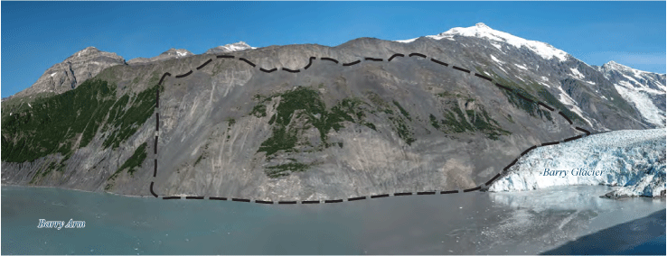
Panoramic photograph of the Barry Arm landslide, with the Barry Glacier terminus (north) to the right. The black dashed line indicates the approximate subaerial extent of the landslide complex. Photograph by Andrew Collins, U.S. Geological Survey.
The geology at Barry Arm is composed primarily of turbidite sequences of the Late Cretaceous Valdez Group represented by variably interbedded sandstone, siltstone, and mudstone flysch (summarized in Wilson and Hults, 2012). These rocks were deposited as part of the Chugach accretionary complex. The rocks are extensively fractured due to multiple subsequent episodes of tectonic deformation, as evidenced by extensive multiscale folding and faulting. Joint sets of varied orientation weaken the rock ubiquitously, with some throughgoing adverse joint sets likely contributing to local slope instability (Schaefer and others, 2023; Coe and others, 2024). Bedding generally strikes southwest and dips moderately to the northwest.
The nearest population center to Barry Arm is Whittier, Alaska, approximately 50 km to the southwest (fig. 1A). The land around Barry Arm lies within the Chugach National Forest, and development since the cessation of mining activities has been limited; however, the area is popular for recreation and commercial fishing. Large commercial cruises frequent Port Wells, Harriman Fiord, Barry Arm, and College Fiord. (Note: the U.S. Board of Geographic Names uses the spelling “Fiord” in proper names. We therefore use this spelling for proper names and the more common spelling, “fjord,” elsewhere). Motorized and nonmotorized small craft also use inlets and bays, and camping is popular on beaches and in low-lying areas along the coast. Therefore, the volume of the Barry Arm landslide, and the size of a potential resultant tsunami wave (Barnhart and others, 2021; Barnhart and others, 2022), has major implications for the region.
Methods
We used the mHVSR method (Nogoshi and Igarashi, 1970, 1971; Nakamura, 1989) to calculate the ratio of smoothed Fourier amplitude spectra of the horizontal component of surface ambient seismic noise to those of the vertical component. This method enabled us to identify (1) f0, or the lowest frequency at which a substrate naturally vibrates, which is controlled by the thickness and mean seismic velocity of lower density layers (like soil) overlying a higher density base (like bedrock) and (2) higher mode resonance frequencies resulting from impedance contrasts between shallower layers in the subsurface (for example, Fäh and others, 2001; Molnar and Cassidy, 2006; Mihaylov and others, 2016). We then used earthquake-derived eHVSR (Lermo and Chávez-García, 1993) and SSR (Borcherdt, 1970) methods to verify the stability and geologic sourcing of these peak frequencies.
We estimated f0 using both HVSRs and Rayleigh wave ellipticity. Ellipticity is understood to show f0 more accurately than HVSR because, as Rayleigh waves are the primary contributor to the shape of the HVSR curve (Lachet and Bard, 1994; Fäh and others, 2001), the ellipticity method removes the complex effect of signals from other types of waves (Fäh and others, 2009). However, this comes at the expense of lower accuracy at peak frequencies above f0, that is, at shallower interfaces. If shallower interfaces can be constrained by seismic velocity or other parameters, this tradeoff can be mitigated (Scherbaum and others, 2003; Fäh and others, 2003, 2009; Wathelet and others, 2004). We calculated Rayleigh wave ellipticity and compared the peak frequencies against mHVSR, eHVSR, and SSR curves to evaluate the stability of peak frequencies and assess the efficacy of the ellipticity as a means to estimate f0 and conduct subsequent analyses.
In the simple case of a uniform, lower density soil layer overlying a strongly contrasting, higher density layer like bedrock, f0 can be used with the shear wave velocity (VS) to estimate the thickness (h) of the overlying material, as shown in equation 1:
For the requirements of equation 1, we assumed the landslide could be modeled as a lower density layer representing damaged, mobile slide-block material overlying a strongly contrasting, higher density base, with VS representing undamaged material below the failure surface (for example, Hartzell and others, 2017; Ma and others, 2019). Using this relation, we inverted the ellipticity curve to model the approximate depth of geologic interfaces.
Seismic Data Selection and Review
Seismic data for this study came primarily from seismometers at stations BAW and BAE of the Alaska Geophysical Network (AEC, University of Alaska Fairbanks, 1987; fig. 1B). The AEC installed BAW on September 4, 2020, on a bedrock knob in the central portion of the Barry Arm landslide (fig. 1B). The station was destroyed by an avalanche on April 18, 2021, after experiencing intermittent reliability issues since mid-December 2020. Station BAE served as our reference station for standard spectral ratio calculations and is located 2.5 km to the southeast of BAW, across the fjord and on top of a bedrock ridge. Station BAE was also installed by AEC on September 4, 2020, and remains operational as of July 2024. Both stations consist(ed) of a triaxial broadband posthole seismometer (Nanometrics Trillium 120) with a 50-hertz (Hz) sample rate. A third station, BAT, was installed on July 23, 2021, to replace BAW; however, due to concerns about hazards at the original site, BAT was installed on the ridge top above the landslide. Instrumentation and sample rate are the same for BAT as for BAW. Records from BAT and BAW do not overlap in time, and BAT is not directly on the landslide. However, we used data from BAT in this study to assess potential effects of local noise sources on the site.
Ambient Noise Data
For calculation of mHVSR, we collected continuous seismic data for the aforementioned sensors using the ObsPy Python utility (Beyreuther and others, 2010). To investigate geophysical changes at the site on a monthly scale, we first reviewed temporal trends by investigating one continuous 24-hour sample of seismic data for each month that BAW and BAE were both transmitting at least part of the time. These are referred to in this report as “monthly data.” These data span September 2020 through April 2021 for BAW and September 2020 through early January 2021 for BAE. The 24-hour sample length mitigated the potential effects of diurnal factors like tides and temperature on the ambient wavefield. We used an interval of 30 days between samples, with ±1-day adjustments as needed in the case of data gaps. This enabled us to identify noteworthy changes in the data across multiple months without storing, managing, and analyzing a continuous record. We investigated monthly data from BAT for a similar but later operational period (September through December 2021) to use for comparative studies.
To provide insight into the rate and potential drivers of daily-scale geophysical changes, we also conducted continuous analysis of spectral characteristics, including computing daily spectrograms to evaluate changes in the mHVSR curve through time, both on and off the landslide. We reviewed all seismic records for completeness and quality. Periods during which seismic stations were out of communication on the scale of days to weeks or were experiencing other data issues (for example, excessive deviations from the prescribed sampling frequency; fig. 3) were excluded from high-resolution analyses. We excluded 2021 data from BAW from the continuous analysis because of reliability issues (likely related to weather interference to the power supply or telemetry equipment) that started in December 2020.
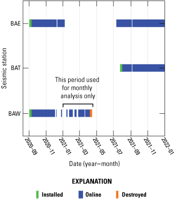
Data availability for BAE, BAT, and BAW seismic stations between September 4, 2020, and January 1, 2022. BAW seismic station was destroyed by an avalanche in April 2021. BAT was installed as a replacement for BAW seismic station in July 2021. Both BAE and BAT seismic stations continue to operate as of July 2024.
Earthquake Data
To calculate eHVSR and SSR to use in comparison against mHVSR results, we selected earthquakes that were recorded on BAE and BAW during the study period from the Advanced National Seismic System Comprehensive Earthquake Database (ComCat) maintained by the U.S. Geological Survey (U.S. Geological Survey, 2017) using the Python library: libcomcat (Hearne and Schovanec, 2020). Using earthquake signals instead of ambient noise for these two methods, and ensuring the peak frequency results are comparable, helps confirm that the mHVSR results are not contaminated by problematic local noise sources because the input waveforms are dominated by signals from a known earthquake source. We selected only earthquakes that occurred in a zone 15–500 km from the central point between BAE and BAW (a distance of approximately 2.5 km; fig. 1B). A minimum distance of 15 km was chosen to minimize potential differences in path effects (Borcherdt, 1970). We used catalogued earthquakes of all magnitudes because fewer than 15 percent of the earthquakes catalogued during the short time that BAW was recording exceeded a magnitude (ML) of 2.0; thus, we determined that no practical magnitude threshold could be established that would not greatly limit the temporal and spatial distribution of data.
For SSR calculations, we selected only earthquakes that were detected at both BAE and BAW and for which S-wave arrival times were recorded or picked. Because of its location near the landslide, BAE was used as the reference station. Filtering by these criteria resulted in 469 applicable earthquakes that spanned September 4, 2020, to January 6, 2021 (after which BAE was offline for an extended period) and ranged in magnitude from 0.5 to 4.7 with a median of 1.4.
HVSR Computation and Parameters
Several software packages were used to complete HVSR analyses. We first used Geopsy (SESAME, 2005; Geopsy Project, 2020) with the monthly datasets to manually adjust parameters and determine the best processing workflow. We also used the final Geopsy results for the inversion. Bulk calculations from large volumes of data for mHVSR, eHVSR, and azimuthal HVSR were performed using the hvsrpy package developed by Vantassel (2021), which is methodologically consistent with Geopsy where their capabilities overlap. For each program, we drew parameters from the software documentation (SESAME, 2005; Vantassel, 2021) or interpreted them based on previous studies (Cara and others, 2003; Martino and others, 2020; Wang and others, 2021; Maresca and others, 2022; Molnar and others, 2022). These parameters are detailed in table 1.
Table 1.
Parameters used for microtremor horizontal-to-vertical spectral ratio calculations in Geopsy (SESAME, 2005; Geopsy Project, 2020) and hvsrpy (Vantassel, 2021).[%, percent; °, degree]
Geopsy uses a log width factor as the constant for Konno-Ohmachi smoothing, whereas hvsrpy uses the exponent “b” as published in Konno and Ohmachi (1998). These values are related by the following equation 2:
Rayleigh wave ellipticity, which relates strongly to the HVSR but mitigates the complicating contributions of Love and body waves, is frequently used to invert for peak frequencies (for example, Fäh and others, 2001; Scherbaum and others, 2003; Wathelet and others, 2004). To derive the ellipticity curve, we used the HVSR time-frequency analysis (HVTFA) and Max2Curve utilities in Geopsy. Although the output of the classical HVSR and HVTFA methods is similar, the HVTFA method uses a continuous wavelet transform (CWT) method to compute the frequency domain signal rather than the Fourier transform. The CWT method requires a different set of parameters (table 2) but is better suited to isolate and analyze spectral maxima in the vertical component, which is assumed to be dominated by Rayleigh wave motion (Fäh and others, 2009). Due to a compatibility issue in the most recent version of Geopsy (3.4.2), Max2Curve steps were implemented in a previous version (2.5; Geopsy Project, 2011) as recommended by Marc Wathelet (Institut des Sciences de la Terre, Centre National de la Recherche Scientifique, and Institut de Recherche pour le Développement, written commun., 2022). All other Geopsy procedures were performed in version 3.4.2 (Geopsy Project, 2020). Parameters for HVTFA and Max2Curve are listed in table 2. For most parameters, the recommendations by Fäh and others (2009) were followed; minimum and maximum histogram values were adjusted to optimize the number of data points captured.
Peak Stability Analysis
To assess the potential effects of various external factors on the mHVSR curve prior to using it to estimate the seismic velocity model, we evaluated the stability of peaks in the curve through time and space. We compared monthly noise curves from BAW to determine if peak amplitude and frequency changed through time between when the station was installed (September 2020) and when it was destroyed (April 2021). We calculated mean curves from BAE and BAT and compared peak frequencies to those at BAW to try to detect consistent and pervasive noise sources like topographic resonance, glacier- or ocean-sourced noise, or atmospheric phenomena that may obscure or otherwise affect the ambient signal. Comparing eHVSR curves and mHVSR curves aided these analyses by demonstrating synchrony between their respective peak frequencies.
We used BAW as the source station and BAE as the reference station to calculate the SSR from earthquake data (Borcherdt, 1970) as another means of verifying peak frequencies. The SSR relies on a common wave train between the source and reference stations, which we derived by isolating the S-wave component at each station for each earthquake. Although the SSR and HVSR are not necessarily expected to match, several studies (for example, Horike and others, 2001; Satoh and others, 2001) have noted that they reliably agree around f0—especially when f0 occurs around or less than 1 Hz—and can agree at higher frequencies (for example, Lermo and Chávez-García, 1993).
Inversion
Analog Material Properties
Inversion of either the HVSR or ellipticity curve to derive the depth profile requires constraints on S-wave velocities of the layer materials. Constraints in the shallow subsurface are especially important for inverting the ellipticity curve (Fäh and others, 2009). As with many unstable slopes, no subsurface exploration or geophysical measurements (for example, refraction-based S-wave profiles) have been conducted at the Barry Arm landslide because of hazardous site conditions; however, surface-rock mass-quality data, including rock quality designation (RQD; Deere and others, 1967) and geologic strength index (GSI; Hoek, 1994; Marinos and Hoek, 2001), were collected at Barry Arm during the 2021 field season (Coe and others, 2024). These data were used as a basis from which to compare material properties to previous studies at sites with similar characteristics where seismic wave velocities were measured. The GSI is somewhat subjective, and RQD can vary considerably in space even on local scales, so both metrics were used for comparison. Three sites near the landslide (fig. 1B) were chosen as representative of a potential range of landslide subsurface material properties (table 3).
Jug and others (2020) provided S-wave velocities for Paleogene flysch sites in Croatia with corresponding GSI and RQD values. Sites used for reference are summarized in table 4. These values are in broad agreement with other authors who have noted S-wave velocities of roughly (~) 350–1,600 meters per second (m/s) in near-surface (upper boundary at 0–60 meters [m]), weathered or highly heterogeneous flysch formations (Gosar and others, 2001; Gosar and Martinec, 2008; Harba and Pilecki, 2017; Totani and Aloisio, 2023). The variability in these ranges corresponds to the degree of weathering, pervasiveness of fracture networks, relative proportions of differently sized particles (for example, sand or clay), and other geologic factors, with more weathered, heterogeneous rock generally corresponding to slower velocities (Jug and others, 2020). Some studies have found higher velocities for deeper flysch (for example, Marcucci and others [2019] modeled a mean S-wave velocity [VS] of 1,750 m/s in a flysch layer 500–1,600 m in depth), but data are sparse for this parameter.
Table 4.
Summary of rock properties and corresponding S-wave velocities collected by Jug and others (2020), with comparable sites from Coe and others (2024) listed.[%, percent; m/s, meter per second]
| Site name | Rock quality designation (%) | Geologic strength index | S-wave velocity (m/s) | Comparable sites from Coe and others (2024) |
|---|---|---|---|---|
| M1 | 15–30 | 20–35 | 250–350 | JAC-03-2021-06-16, JAC-04-2021-06-16 |
| M2 | 35–70 | 40–60 | 350–600 | JAC-02-2021-06-17 |
| S2 | 15–30 | 15–25 | 300–500 | JAC-03-2021-06-16, JAC-04-2021-06-16 |
| S3 | 50–70 | 40–45 | 600–900 | JAC-02-2021-06-17 |
Inversion Modeling
We chose the September ellipticity curve (fig. 4) for inversion based on the well-defined curve, relative lack of transient seismic events, and because it was one of the best-quality monthly curves estimated, passing 3 of 3 criteria for peak reliability and 5 of 6 criteria for peak clarity suggested by SESAME (2005), thereby meeting their classification of “very reliable.” Once we established the final parameter set, we also inverted the October curve to check for consistency. The Dinver utility in Geopsy was used to invert the ellipticity curve to find the seismic velocity model, and we were especially interested in constraining the depths of interfaces. Dinver uses a modified version of the neighborhood algorithm (Sambridge, 1999a, 1999b) to search for all possible solutions in an n-dimensional parameter space with a user-defined parameter that determines the total number of iterations of model selection (Ns), number of initial models randomly sampled from the parameter space (Ns0), and models to consider when resampling (Nr) (Wathelet and others, 2005; Wathelet, 2008; Vantassel and Cox, 2021). These parameters are used to define how much free range the algorithm has to find different solutions at the outset and then to control how the algorithm selects the best fit. For these analyses, we assigned the Dinver default values Ns0=50, Ns=10,000, and Nr=50 to exploratory runs. We used values suggested by Vantassel and Cox (2021): Ns0=100, Ns=50,000, and Nr=100 to verify convergence for the best-fitting model results.
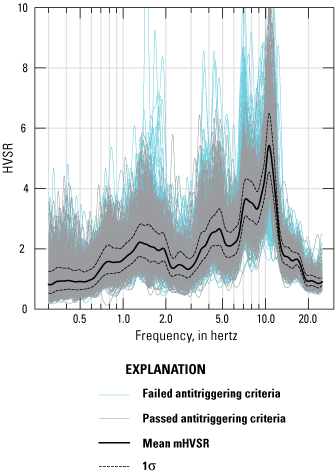
Microtremor horizontal-to-vertical spectral ratio (mHVSR) curve (mean of all windows) at BAW seismic station for the 24-hour period beginning September 9, 2020, 08:00:00 Coordinated Universal Time. Peaks are evident at 1.5 hertz (Hz), 4–5 Hz, and 7–11 Hz. (HVSR, horizontal-to-vertical spectral ratio; σ, standard deviation)
Using the September ellipticity curve, we constructed 3-, 4-, and 10-layer models. The 3- and 10-layer models were based on the minimum and maximum interpretations, respectively, of the number of peaks present in the September 2020 ellipticity curve at BAW. The 4-layer configuration was based on our hypothesis that each major peak in the HVSR might represent a layer boundary, such that three major peaks would indicate four layers including a half-space.
We explored a range of possible parameter values tied to analogs and known rock properties to maximize the potential for a close curve fit in the absence of subsurface calibration data. Ranges used for each parameter across all layer and parameter-space configurations are shown in table 5. We assumed that the layers within the slide block (0 and 1 in the 3-layer model; 0, 1, and 2 in the 4-layer model) were analogous to values found in the literature (Gosar and others, 2001; Gosar and Martinec, 2008; Harba and Pilecki, 2017; Jug and others, 2020; Totani and Aloisio, 2023). Because relatively little is known about the geology within and beneath the Barry Arm landslide, the maximum values used in the model were higher than the maximum values referenced in the literature by a factor of ~2, assuming higher densities and fewer discontinuities at depth. Density was varied to allow for the range of fractured mudstone to coherent sandstone constituents. Because the Dinver results are most sensitive to S-wave velocity and density, we used Dinver’s generalized default values for P-wave velocity and the Poisson’s ratio. Dinver uses the Poisson’s ratio to govern the relation between P-wave velocity (VP) and VS such that unrealistic combinations are not allowed. Still, we verified that, for all model runs, the algorithm never explored unreasonable relations between VP and VS. For example, we verified that no models were run where VP=VS in the shallow subsurface. The minimum VP explored among all model iterations was approximately 300 m/s (corresponding to VS=200 m/s) within the slide block and approximately 1,000 m/s below the primary failure surface (corresponding to VS=700 m/s).
Table 5.
Summary of input parameter ranges across all starting model parameter space sets.[VP, P-wave velocity; m/s, meter per second; VS, S-wave velocity; kg/m3, kilogram per cubic meter; m, meter; N/A, not applicable]
We tested 24 unique starting model parameter space sets for the 3-layer model, 14 for the 4-layer model, and 6 for the 10-layer model. We ran each parameterization at least three times to verify that differences in initial model selection by the neighborhood algorithm would not generate meaningfully different results. To quantify uncertainty in our VS profile results, we computed the standard deviation of output values for interface depth for all model iterations based on the best-fitting starting parameter space with a misfit less than the median. The misfit in Geopsy’s Dinver module is calculated as shown in equation 3:
wherexdi
is the velocity of the input data curve at frequency fi,
xci
is the velocity of the calculated curve at frequency fi,
σi
is the uncertainty estimate of the frequency samples considered (Wathelet and others, 2004), and
nF
is the number of frequency samples considered.
Results and Discussion
HVSR
Peak frequencies in the mHVSR and eHVSR curves at the BAW seismometer site were consistently identified at approximately 1.5 Hz, 4–5 Hz, and in a double peak at 7–11 Hz in the frequency spectrum (fig. 5). Peak frequencies remain consistent through time; however, a marked and sustained change in amplitude of the 7–11-Hz peaks was noted between the October and November monthly curves. The possible causes are explored later in this section, but because of this change, we opted to evaluate peak stability within two separate timeframes: September and October 2020 (preshift), and November 2020 to April 2021 (postshift). The preshift timeframe is considered here to be the reference condition. The monthly curves from this period represent initial conditions for the study and are more likely to pass reliability criteria established by SESAME (2005) due to the higher peak amplitudes and differentiable peak shapes. The September monthly curve demonstrates these characteristics and is shown in greater detail in figure 4.
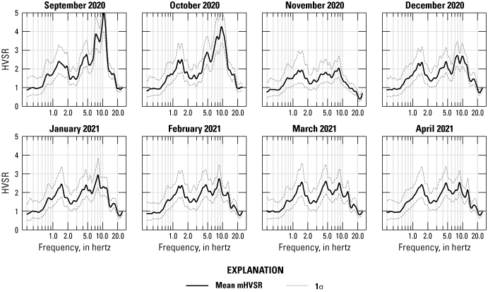
Monthly microtremor horizontal-to-vertical spectral ratio (mHVSR) curves for September 2020 through April 2021. The amplitude, especially of the 4–5-hertz (Hz) and 7–11-Hz peaks, changes through time, but the location of the peaks remains broadly consistent. (HVSR, horizontal-to-vertical spectral ratio; σ, standard deviation)
The highest amplitudes in the preshift timeframe manifest as a double peak in the 7–11-Hz range, with the higher-frequency peak (amplitude ~5 in September) centered on approximately 10 Hz and the lower frequency subpeak (amplitude ~4 in September) centered between 7 and 8 Hz (figs. 4, 5). In November and December, the amplitudes of these higher frequency peaks reduce to the amplitude of the other peaks in the curve (amplitude ~2 in November), although the peak frequencies remain approximately consistent. In January through April 2021, the double-peak shape is replaced by a single peak fluctuating between 7 and 8.5 Hz with shoulder peaks at approximately 11 and 18 Hz. These shoulder peaks were present but less pronounced in preceding samples. A trough at 20 Hz is consistent through time.
The lowest frequency and lowest amplitude peaks were centered around 1.5 Hz consistently through time. In the case of multiple HVSR peaks, we assume the lowest frequency peak (1.5 Hz at BAW) represents f0 and that it reflects the impedance contrast at the boundary between damaged (mobile) and undamaged material (for example, Guéguen and others, 2007; Mihaylov and others, 2016). The consistent locations of the primary peaks through time reinforce the veracity of these peak frequencies, especially in the 1.5-Hz peak, which shows the least temporal and amplitude variability.
All three peaks occur at similar frequencies and show similar behavior through time in earthquake and noise ratios (fig. 6). In both ratios, the 1.5-Hz peak appears stable through time, whereas the 7–11-Hz peaks (and, to a lesser degree, the 4–5-Hz peak) reduce in amplitude in the postshift period. The 7–11-Hz peaks also consolidate from double to single peaks in the 7–8-Hz range between timeframes in both earthquake and noise calculations.
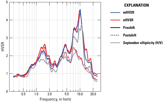
Median microtremor horizontal-to-vertical spectral ratio (mHVSR) from monthly curves compared with the median earthquake horizontal-to-vertical spectral ratio (eHVSR) curves from all earthquakes recorded at BAW and BAE seismic stations during the study period. Data are grouped relative to the change in the shape of the curve at BAW seismic station. The time-grouped curves are similar in shape and amplitude, and the peak frequencies are broadly consistent between all groups. The ellipticity curve from September noise data is comparable in shape and amplitude to the preshift horizontal-to-vertical spectral ratio (HVSR) curves. (H/V, horizontal over vertical)
The Rayleigh wave ellipticity results match closely with the classical mHVSR and eHVSR values. Peaks similarly occur at 1.5 Hz, between 4 and 5 Hz, and between 7 and 11 Hz (fig. 6). The ellipticity curve is considered most reliable for inversion modeling between f0 (1.5 Hz) and the minimum of the trough to the right of f0 (Fäh and others, 2009), which is between 2 and 3 Hz in this study. In this case, the stability of peak frequencies across multiple methods of analysis (mHVSR, eHVSR, SSR, ellipticity) lends confidence to the usability of these parts of the curve.
We computed the mHVSR at BAE (even though it is not on the landslide) to evaluate its quality as a reference site for SSR and to examine if there were any shared peaks with BAW that might indicate local resonant noise sources. The result shows that BAE also has signs of site amplification but not at the same frequencies as BAW, so these effects are likely local to the BAE site. The computed result for BAE shows a primary peak occurring at approximately 2.5 Hz and additional low-amplitude peaks occurring around 5–7 Hz and at approximately 9–10 Hz (fig. 7A). We also investigated BAT (even though it was installed after BAW was destroyed and could not be used as a reference site) to determine if some peaks may be related to local noise sources, in which case they would show up on all sensors. Results from BAT indicate a low-amplitude double peak at 5–6 Hz (fig. 7B). The peak frequencies differ between the three seismic stations such that no common resonant noise sources are evident in the amplitude and frequency ranges evaluated.
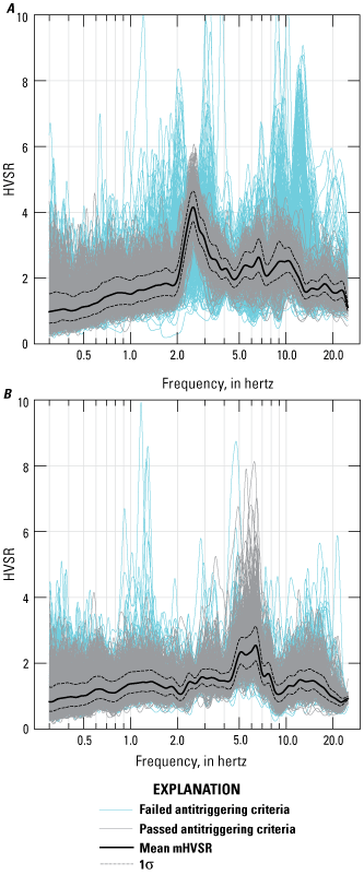
Representative microtremor horizontal-to-vertical spectral ratio (mHVSR) curves for A, BAE seismic station and B, BAT seismic station. BAE seismic station shows a primary peak at 2.5 hertz (Hz) and additional low-amplitude peaks at 5–7 Hz and 10 Hz, and BAT seismic station shows a consistent peak at 5–6 Hz. The differences in peak frequencies between these seismic stations and BAW seismic station likely indicates that the BAW seismic station peaks are stratigraphic in origin. (HVSR, horizontal-to-vertical spectral ratio; σ, standard deviation)
The computed SSRs between BAW and BAE show a similar change between pre and postshift timeframes, wherein the higher frequency peaks in the SSRs reduce in amplitude and some consolidation occurs (fig. 8). For both the preshift and postshift datasets, a peak at 1.5 Hz is consistently represented in the SSRs. A 4–5-Hz peak shows very slightly in the SSRs computed from the east (E)–west (W) components, whereas a peak of similar amplitude shows at between 5 and 6 Hz in the north–south SSRs. The higher frequencies (7–11 Hz and higher) in the SSRs contain more peaks and complexity than in the HVSRs, but the 7–11-Hz peaks are well represented in the preshift SSRs, especially in the E–W components. Postshift, a peak is present at 7 Hz, but additional peaks in the 12–20-Hz range have higher amplitudes.
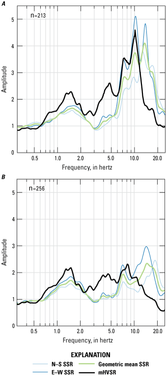
Three-component standard spectral ratios (SSRs) using BAW as the source seismic station and BAE seismic station as the reference site for the periods of A, September through October, and B, November through December 2020. Each horizontal component SSR (north [N]–south [S] and east [E]–west [W]) is shown with the geometric mean of the two. The sample size (n) for the period from September to October is 213 earthquakes; 256 earthquakes were used for the period from November to December. The agreement in the SSRs and microtremor horizontal-to-vertical spectral ratio (mHVSR), particularly at the 1.5-hertz (Hz) peak, indicates that the peak frequencies are stable and representative of subsurface structure.
With such complex topography, topographic resonance as a potential source of low-frequency peaks (Geli and others, 1988; Hartzell and others, 2014; Weber and others, 2022) cannot be definitively ruled out. We investigated the likelihood of its effect using the relation shown in equation 4:
wherefa
is the maximum amplification frequency due to topographic resonance of a contributing source,
VS
is the mean bedrock S-wave velocity, and
L
is the base width of the topographic feature (Hartzell and others, 2014).
Considering a possible S-wave velocity range for the feature between 900 m/s (equal to the highest velocity estimate for flysch provided by Jug and others [2020]) and 2,800 m/s (a conservative estimate based on the results of this study), the maximum frequency of topographic resonance at BAW is likely between 0.1 and 0.4 Hz. This value is much lower than the lowest HVSR peak at 1.5 Hz. The differing peak HVSR frequencies between the three seismic stations and the stability of the HVSR peak frequencies at BAW through time and across methods indicate that, despite the site complexity and numerous potential contributing noise sources, the peaks in the HVSR curves at BAW are stratigraphic in origin and not due to local noise sources. The agreement between HVSRs and SSRs—inclusive of changes to the curve shape—corroborates this conclusion.
We next investigated the cause of the change in curve shape between October and November 2020 at BAW to determine if it provides meaningful information about the landslide or simply reflects seasonal changes. Using a spectrogram-like visualization of the mHVSR computed with continuous data, a discrete shift is visible around October 30 (fig. 9). Movement of the landslide was ongoing throughout the month of October according to interferometric synthetic aperture radar (InSAR) data (Schaefer and others, 2020) and light detection and ranging (lidar) differencing (Schaefer and others, 2023); however, the temporal resolution of these methods is not high enough to determine precisely when motion was occurring.
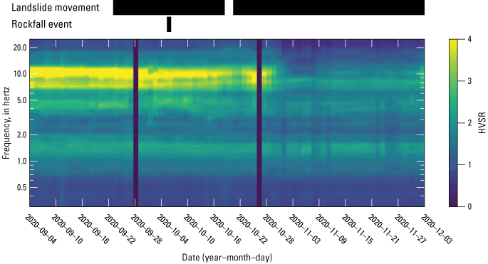
Spectrogram of continuous daily seismic data from BAW seismic station. Microtremor horizontal-to-vertical spectral ratio (mHVSR) amplitude is represented on a time compared to frequency plot as a color ramp with yellow equating to higher amplitudes and blue equating to lower amplitudes. Time windows within which landslide deformation and a large (roughly 650,000 cubic meters) rock avalanche (Schaefer and others, 2023) occurred are also shown in separate black bars above the spectrogram. The time windows of landslide deformation are derived from interferometric synthetic aperture radar and light detection and ranging (lidar) differencing; due to the low temporal resolution of these methods, the exact dates of movement are unknown (Schaefer and others, 2020, 2023). A marked decrease in mHVSR amplitude in the 7–12-hertz (Hz) bandwidth is evident around October 30, with no apparent recovery. This decrease does not seem attributable to hydrologic, glacial, or seasonal changes, but may relate to changes in the subsurface structure due to landslide motion or decoupling of the sensor. (HVSR, horizontal-to-vertical spectral ratio)
We also considered weather as a potential external driver of geophysical change. We reviewed daily wind, precipitation, and temperature data from the two nearest Snow Telemetry (SNOTEL) stations (U.S. Department of Agriculture National Water and Climate Center, 2017) to the landslide. These stations are each approximately 50 km from the landslide and were the only sources of continuous high-resolution weather data we found. We noted that temperatures started to drop below freezing consistently at night at both SNOTEL stations between October 28 and October 30, so one possibility is that the geophysical change around this time (fig. 9) could be due to the seasonal freezing of shallow surface layers, which would change the shallow seismic velocity profile (for example, James and others, 2019; Miao and others, 2019) and thus alter the HVSR profile at higher frequencies. Absent a longer available seismic record at this site, this potential correlation is difficult to establish. There is not a similar change at sites BAE or BAT, but these sites are on ridge tops and may have less near-surface water content, so it is not an ideal comparison between BAW and BAE or BAT. No other relation between weather at these SNOTEL stations and changes in the seismic wavefield was immediately evident; however, because the weather is often highly variable over localized spatial scales in and around Prince William Sound, the conditions at the stations may not be comparable to the conditions at the landslide.
During the study period, small rockfall events are abundant in the seismic record, and a large (~650,000 m3) rock avalanche on October 5 in the central part of the landslide narrowly missed BAW (Schaefer and others, 2023). Deep landslide-wide deformation also occurred around this time, and it is possible that the coupling between the sensor and the surrounding soil was reduced or altered during that period of motion, resulting in a fundamental change in the shape of the HVSR curve. We reviewed the state-of-health records for the sensor at BAW for motion anomalies occurring around the time of the change, and none were evident, but the accuracy of those measurements is low.
Transient shifts, such as the undulation in the mHVSR curve in the 4–5-Hz band around the beginning of October (fig. 9), may also reflect structural changes in the material underlying the receiving seismometer. Other authors (Gaffet and others, 2010; Mainsant and others, 2012; Uhlemann and others, 2023) have noted geophysical evidence of structural changes in unstable slopes in the hours and days leading up to slope failure. The noteworthy and sustained change in the mHVSR curve at BAW at the end of October 2020 may reflect a major event during an episode of ongoing deformation of Barry Arm. The lack of any similar changes observed in the records at BAE and BAT rules out regional-scale effects on noise sources like hydrologic or glacial changes and possibly supports a local structural cause; however, the temporal-coverage limitations of corroborating sources like InSAR at BAW make determination difficult.
Inversion
We found the 4-layer seismic velocity model to best reflect the general shape of the representative September 2020 BAW ellipticity curve with the lowest level of complexity (fig. 10). From 14 different parameter sets initially modeled, we ran the one that produced a model with the lowest overall misfit (0.072) three more times with more initial flexibility and more iterations to verify convergence (Vantassel and Cox, 2021). The mean minimum misfit of the verification runs was 0.067. The input parameter ranges for the parameter set that produced best-fitting model are summarized in table 6. When we inverted the ellipticity curve for a 3-layer model, we were unable to find a solution that adequately reflected the number or shape of peaks in the mHVSR curve. The 10-layer model, despite its increased complexity, did not improve the curve fit. The minimum misfit achieved for the 3-layer model was 0.19, and the minimum misfit for the 10-layer model was 0.12.
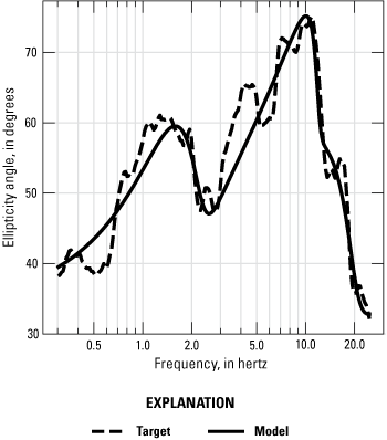
Target ellipticity curve with modeled output curve from the mean best-fitting model. The output curve correlates well with the input, especially at the 1.5-hertz (Hz) and 7–11-Hz peaks. The 4–5-Hz peak was not adequately captured by any 3-, 4-, or 10-layer inversions modeled in this study.
Table 6.
Summary of input parameter ranges for best-performing parameter space for the 4-layer inversion of September 2020 BAW ellipticity curve.[VP, P-wave velocity; m/s, meter per second; VS, S-wave velocity; kg/m3, kilogram per cubic meter; m, meter; >, greater than; N/A, not applicable]
The mean result of the best-fitting model run and three verification runs converged on a bottom interface depth of 188 m below the ground surface, with additional velocity contrasts at 4.4 and 20.5 m below the ground surface. These results are shown in figure 11 and detailed in table 7 along with additional model outputs.
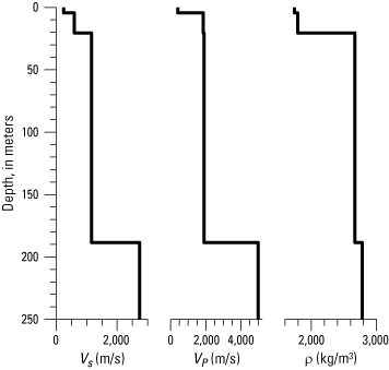
S-wave velocity (VS), P-wave velocity (VP), and density (ρ) profiles of the mean best-fitting inversion model from the September 2020 ellipticity curve. Velocity and density contrasts are present at 4.4, 20.5, and 188 meters below ground surface. (m/s, meter per second; kg/m3, kilogram per cubic meter)
Table 7.
Best-fit result of 4-layer inversion of the September 2020 BAW ellipticity curve.[m, meter; VP, P-wave velocity; m/s, meter per second; VS, S-wave velocity; kg/m3, kilogram per cubic meter; N/A, not applicable]
The comparison of the modeled curve with the target ellipticity curve is shown in figure 10. The base of layer 2 at approximately 188 m below ground surface (fig. 11) is likely to reflect the 1.5-Hz peak and the impedance contrast between coherent bedrock and damaged or displaced overlying material (fig. 10). This depth represents the estimated thickness of the slide mass in slope-normal profile relative to the BAW site. The intermediate contrasts in the profile may represent additional layer boundaries within the damaged and potentially mobile material. Notably, the 4–5-Hz peak of the ellipticity curve is not well captured by the model; no 3-, 4-, or 10-layer parameter configuration we tested was able to capture it. Because this peak was also reduced in or absent from the SSR curves, and peaks at similar frequencies are present in the BAE and BAT HVSR curves (fig. 7), the peak may be related to a noise source rather than a stratigraphic one. We avoided forcing narrow parameter constraints due to the lack of geologic constraints on the data.
The 4-layer inversion of the October ellipticity curve, which we modeled using the same parameters as the September curve, achieved similar results (table 8), albeit with a slightly higher misfit (0.10), which is possibly attributable to more transient events in the October noise record.
Table 8.
Comparison of inversion results for September and October ellipticity curves.[mHVSR, microtremor horizontal-to-vertical spectral ratio; bn, thickness of layer n; m, meter; m/s, meter per second; VSn, S-wave velocity of layer n]
The indication of multiple layers is plausible for a bedrock landslide, where materials may be moving at different rates due to differential pressures, hydrologic conditions, material strengths, fracture densities, or other factors (for example, Yerro and others, 2016). The stability of the 1.5-Hz peak signifies the location of a primary failure surface at a depth that is consistent through time. Changes to the properties or seismometer coupling with a talus layer on the surface of the Barry Arm landslide may be reflected in changes in the higher frequency peak amplitudes, whereas amplitude changes in the 4–5-Hz range may reflect internal deformation of the slide mass.
Inversion Uncertainty
Inversion without calibration targets or reliable geologic constraints is highly nonunique. In an effort to minimize uncertainty under these circumstances, we used multiple methods to verify the stability of peak frequencies in the HVSR curve, constrained material properties (especially at shallow depth) using data from analogous settings, and inverted the ellipticity rather than the HVSR curve. To quantify the uncertainty of the result after applying these constraints, we used an approach similar to that recommended by Vantassel and Cox (2021). We assessed uncertainty qualitatively by plotting all VS profiles with a misfit less than the median (0.10) from each of the four September ellipticity inversion model runs that used the best-fitting starting parameter set (the initial model run and the three verification runs; fig. 12; table 6).
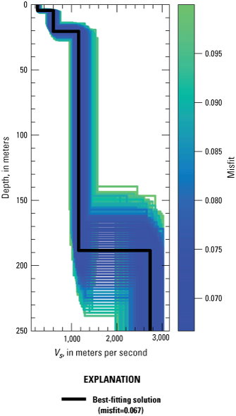
Uncertainty visualized with S-wave velocity (VS) profiles of all model iterations (sample size=84,317) from each of the best-fitting initial parameter spaces with a misfit less than the median misfit, 0.10. Variability in results is notable around the depth of the failure surface; however, agreement generally is good in shape and output values across iterations. The standard deviation of the depth to the landslide failure surface based on this dataset is ±9 meters.
Figure 12 demonstrates, predictably, that uncertainty in velocity increases with depth, as does variability around interface depth. Notably, however, there is generally good agreement between iterations, and the uncertainty is not very high. Although there is no established method to quantify absolute uncertainty in these data, we note that the standard deviation of depth to the landslide failure surface based on the ~84,000 iterations shown in figure 12 is ±9 m around the best-fitting solution of 188 m.
These results, although not constrained by geologic data, are internally consistent given the relatively free range of the model parameter space, the number of parameter sets tested, and the analog property ranges. The results are also consistent with, and an improvement upon, previous modeling work performed at the site that derived log-spiral failure surfaces of the Barry Arm landslide from 45-degree and 60-degree headscarps (Barnhart and others, 2022). Transects from that study passing through the BAW site place the slope-normal depth of the failure surface at 110 and 235 m, respectively, below the ground surface at the BAW site.
Azimuthal Variability
Based on the conclusions of previous studies (for example, Del Gaudio and others, 2014; Matsushima and others, 2014; Hartzell and others, 2017; Perton and others, 2018; La Rocca and others, 2020), we assessed if azimuthal variability in HVSR curves could be used to interpret site structure, like slide mass shape and asymmetry, stratigraphic controls on direction of travel, and overall relation of the slide mass to underlying geologic structure. Deriving rotated components of the September–October mHVSR and eHVSR curves at 15-degree intervals shows decreases in the 4–5-Hz and 7–11-Hz peak amplitude between 30 degrees and 60 degrees, whereas the amplitude of the 1.5-Hz peak stays consistent (fig. 13). The orientations where amplitudes for the 4–5-Hz and 7–11-Hz peaks are higher are approximately parallel to strike-slip faults governing the downslope movement of the Barry Army landslide (Coe and others, 2021; fig. 14) and are approximately perpendicular to the orientation of the main headscarp of the landslide.
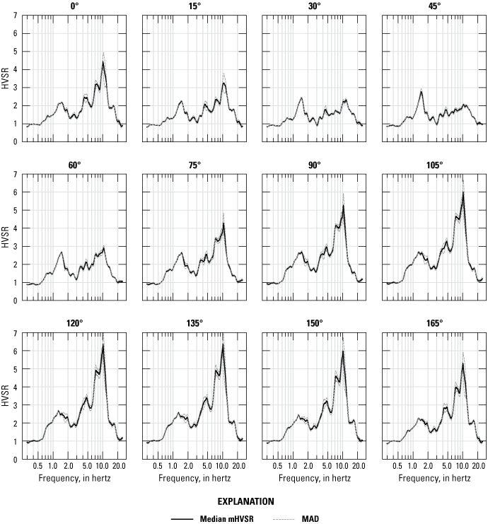
Microtremor horizontal-to-vertical spectral ratio (mHVSR) curves from continuous (September–October) 2020 BAW seismic station noise data reflecting azimuthal variability at 15-degree intervals. A decrease in 7–11-hertz (Hz) peak amplitude between 30 and 60 degrees may reflect effects of landslide geometry and slip-surface orientation. (MAD, median absolute deviation; °, degree; HVSR, horizontal-to-vertical spectral ratio)
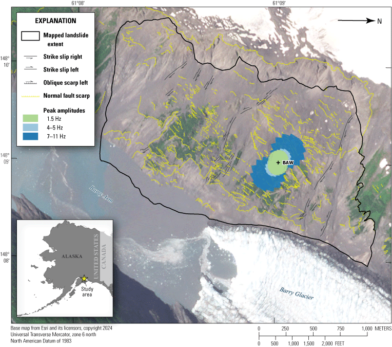
Polar plot showing relative peak amplitudes for each primary microtremor horizontal-to-vertical spectral ratio (mHVSR) peak frequency band at the BAW seismic station at 15-degree intervals overlaid on a map of structural components of the Barry Arm landslide recorded by Coe and others (2021) to illustrate that peak amplitudes, especially in the 4–5-hertz (Hz) and 7–11-Hz frequency bands, are amplified in the orientation parallel to slip. Azimuthal mHVSR amplitudes are calculated at 15 degrees up to 180 degrees and mirrored to create a full 360-degree plot.
The effects of geologic structure on lateral heterogeneity in HVSR curves are not well understood, although many authors have posited that a strong connection exists (for example, Del Gaudio and others, 2014; Matsushima and others, 2014; Hartzell and others, 2017; Perton and others, 2018; La Rocca and others, 2020). Del Gaudio and others (2014) suggested that material weakening due to strain on a landslide slip surface may result in enhanced amplification in the direction of movement, although they also note that topography and structural features likely play a role as well. Tension cracks, which often develop perpendicular to the maximum slope direction (and which occur at various scales at Barry Arm), likely contribute to anisotropy in the slope material and consequently in the seismic signature (Moore and others, 2011; Del Gaudio and others, 2014). Still, the lack of a similar directionality to azimuthal mHVSRs computed for BAT (fig. 15) may indicate that the landslide or hillslope-scale structural features (or both) play a more noteworthy role. These contributions are not well constrained in the existing body of literature.
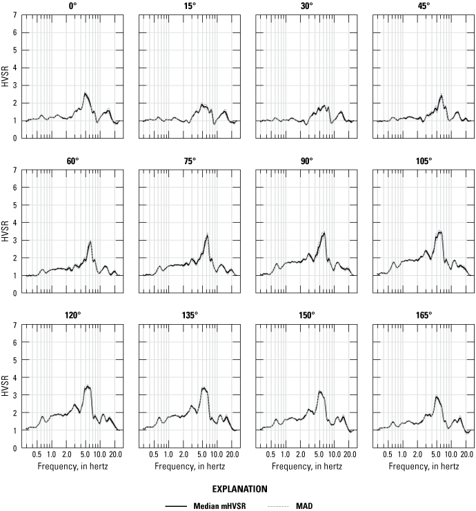
Microtremor horizontal-to-vertical spectral ratio (mHVSR) curves from continuous (September–October) 2021 BAT seismic station noise data showing azimuthal mHVSRs at 15-degree intervals. Because BAT is located on the ridgetop above the former site of BAW but its azimuthal biases appear more muted, it is likely that the azimuthal variability in BAW reflects landslide geometry, hillslope-scale structural information, or both. Amplitude (Y) scale of this figure is kept the same as figure 13 for comparison. (MAD, median absolute deviation; °, degree; HVSR, horizontal-to-vertical spectral ratio)
We evaluated directional response related to earthquakes detected at BAW by visualizing peak amplitudes in representative bandwidths according to earthquake back azimuth (after Hartzell and others, 2014). Some attenuation of eHVSR peak amplitudes was evident in the 7–11-Hz band between 0 and 90 degrees, and asymmetry along the northwest–southeast axis is evident in the 11–15-Hz band where amplitudes along the axis are higher than those perpendicular to the axis (fig. 16). These amplitudes may correlate with the azimuthal variability of the noise data, but no systematic correlation with other parameters was observed.
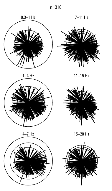
Earthquake horizontal-to-vertical spectral ratio (eHVSR) peak amplitudes as a function of source back azimuth at BAW seismic station. The radius of the middle circle of each bandwidth is proportional to the geometric mean of the eHVSR averaged across 310 (n) earthquakes that were measured by BAW seismic station in September and October 2020. The radii of the outer and inner circles are equal to the geometric mean multiplied and divided by, respectively, the geometric deviation. Spoke length and direction are proportional to the eHVSR amplitude and back azimuth, respectively, for each individual event. The distribution of eHVSR peak amplitudes appears random except for the 7–11-hertz (Hz) frequency band, where amplitudes decrease throughout the northeast quadrant, and the 11–15-Hz band, where amplitudes are higher along a northwest–southeast axis relative to other axes.
Conclusion
In 2019, a large, slow-moving, and potentially tsunamigenic landslide was recognized at Barry Arm fjord in western Prince William Sound approximately 50 kilometers northeast of Whittier, Alaska. Subsequent analysis revealed recent acceleration of the landslide temporally coincident with the rapid retreat of Barry Glacier. With an estimated volume between 290 × 106 and 689 × 106 cubic meters, the landslide could generate a tsunami that could affect high-use waterways and critical harbor infrastructure in Whittier. Direct methods for characterizing landslide depth are impractical for this landslide given the objective hazards and local environmental regulations. Therefore, preliminary hazard models and volume estimates of the landslide have relied on expressions of the headscarp(s) and simplifying assumptions about the subsurface slide geometry, resulting in a high degree of uncertainty. We used a seismometer located on the landslide to constrain the depth of the failure surface with geophysical techniques, thereby improving the existing spread of estimates, which ranges from 110 to 235 meters (m) below ground surface at the location of the seismometer.
We inverted an ellipticity curve derived from seismic noise recorded at the seismometer located on the landslide to estimate the seismic velocity profile and, foremost, the depth of the failure surface. We computed horizontal-to-vertical spectral ratios (HVSR) of seismic microtremors (mHVSR) and earthquakes (eHVSR) as well as ellipticity curves using available seismic records from BAW seismic station located on the landslide. By corroborating the ellipticity curves used for subsurface structure inversion with HVSRs and standard spectral ratios (SSRs), and by eliminating other potential noise sources as contributors using nearby BAE and BAT seismic stations, we established the consistency of three amplitude peaks at 1.5 hertz (Hz), 4–5 Hz, and 7–11 Hz, with 1.5 Hz likely representing the site fundamental frequency and the impedance contrast between undamaged bedrock and overlying slide mass material. The occurrence of similar changes in the HVSRs and SSR at BAW around October 30, 2020, further supports a stratigraphic origin of curve characteristics.
Absent subsurface velocity data for calibration, we constrained seismic velocities based on studies in analogous rock materials using geologic strength index and rock quality designation as points of comparison. We input S-wave velocity (VS) and nonrestrictive depth ranges into Geopsy’s Dinver module to invert the ellipticity curve for interface depth. Based on inversion of the representative September 2020 ellipticity curve, we estimated a slope-normal thickness of the whole slide mass of approximately 188 m, likely divisible into three separate layers of mobile material consisting of a shallow layer 4.4 m thick (possibly talus), a middle layer 16.0 m thick, and a deeper layer 168 m thick. Even with some constraints applied, the chosen inversion model solution is nonunique and there is a high degree of uncertainty; however, good agreement between inversion model iterations, low misfit values, and consistent model results for VS and interface depth between different parameterizations and different time periods give us confidence the main interface depth is within ±9 m of 188 m and indicate this estimate is still likely to be a considerable improvement over current (July 2024) unconstrained estimates.
We also computed azimuthal mHVSRs and eHVSRs at 15-degree intervals at BAW and BAT to investigate underlying structural variability in the landslide. Similar to previous studies, we observed a bias of higher peak amplitudes at BAW approximately parallel to the orientation of slip, which is between 30 and 60 degrees at this site. Analysis of peak eHVSR amplitudes relative to earthquake back azimuth showed similar results, although these results showed less contrast in amplification than the statistical mHVSR azimuthal calculations. A lack of similar directionality at BAT indicates that the landslide, hillslope-scale structural features around the landslide, or both may play more of a role in the shape of the HVSR curve than regional topography. These effects could be further examined in future studies to gain additional insight.
The modeling of the subsurface structure corresponding to these HVSR results is nonunique; however, the internal consistency of our results and their external consistency with limited modeling of landslide sliding-plane depth previously performed in this area give us confidence in the outcome. These results can help constrain information about the Barry Arm landslide geometry and aid in future modeling and site-characterization efforts. Despite topographic and structural complexity, the HVSR method provides usable and repeatable results and can be used as a means of investigation, especially where site conditions preclude more invasive techniques.
References Cited
Alaska Earthquake Center, University of Alaska Fairbanks, 1987, Alaska Geophysical Network [dataset]: International Federation of Digital Seismograph Networks, accessed April 16, 2023, at https://doi.org/10.7914/SN/AK.
Barnhart, K.R., Collins, A.L., Avdievitch, N.N., Jones, R.P., George, D.L., Coe, J.A., and Staley, D.M., 2022, Simulated inundation extent and depth in Harriman Fjord and Barry Arm, western Prince William Sound, Alaska, resulting from the hypothetical rapid motion of landslides into Barry Arm Fjord, Prince William Sound, Alaska: U.S. Geological Survey data release, accessed June 28, 2023, at https://doi.org/10.5066/P9QGWH9Z.
Barnhart, K.R., Jones, R.P., George, D.L., Coe, J.A., and Staley, D.M., 2021, Preliminary assessment of the wave generating potential from landslides at Barry Arm, Prince William Sound, Alaska: U.S. Geological Survey Open-File Report 2021–1071, 28 p., accessed April 26, 2023, at https://doi.org/10.3133/ofr20211071.
Beyreuther, M., Barsch, R., Krischer, L., Megies, T., Behr, Y., and Wassermann, J., 2010, ObsPy—A Python toolbox for seismology: Seismological Research Letters, v. 81, no. 3, p. 530–533, accessed April 16, 2023, at https://doi.org/10.1785/gssrl.81.3.530.
Borcherdt, R.D., 1970, Effects of local geology on ground motion near San Francisco Bay: Bulletin of the Seismological Society of America, v. 60, no. 1, p. 29–61, accessed April 16, 2023, at https://doi.org/10.1785/BSSA0600010029.
Calamita, G., Gallipoli, M.R., Gueguen, E., Sinisi, R., Summa, V., Vignola, L., Stabile, T.A., Bellanova, J., Piscitelli, S., and Perrone, A., 2023, Integrated geophysical and geological surveys reveal new details of the large Montescaglioso (southern Italy) landslide of December 2013: Engineering Geology, v. 313, article 106984, 16 p., accessed April 21, 2023, at https://doi.org/10.1016/j.enggeo.2023.106984.
Cara, F., Di Giulio, G., and Rovelli, A., 2003, A study on seismic noise variations at Colfiorito, central Italy—Implications for the use of H/V spectral ratios: Geophysical Research Letters, v. 30, no. 18, 4 p., accessed April 21, 2023, at https://doi.org/10.1029/2003GL017807.
Coe, J.A., Belair, G.M., Avdievitch, N.N., Lahusen, S.R., Macias, M.A., Collins, B.D., and Staley, D.M., 2024, Rock mass quality and structural geology observations in northwest Prince William Sound, Alaska from the summer of 2021: U.S. Geological Survey data release, accessed July 29, 2024, at https://doi.org/10.5066/P9UBHS4Q.
Coe, J.A., Wolken, G.J., Daanen, R.P., and Schmitt, R.G., 2021, Map of landslide structures and kinematic elements at Barry Arm, Alaska in the summer of 2020: U.S. Geological Survey data release, accessed April 26, 2023, at https://doi.org/10.5066/P9EUCGJQ.
Dai, C., Higman, B., Lynett, P.J., Jacquemart, M., Howat, I.M., Liljedahl, A.K., Dufresne, A., Freymueller, J.T., Geertsema, M., Ward Jones, M., and Haeussler, P.J., 2020, Detection and assessment of a large and potentially tsunamigenic periglacial landslide in Barry Arm, Alaska: Geophysical Research Letters, v. 47, no. 22, accessed April 26, 2023, at https://doi.org/10.1029/2020GL089800.
Deere, D.U., Hendron, A.J., Jr., Patton, F.D., and Cording, E.J., 1967, Design of surface and near-surface construction in rock, in Fairhurst, C., ed., Failure and breakage of rock: New York, Society of Mining Engineers of the American Institute of Mining, Metallurgical, and Petroleum Engineers, Incorporated [AIME], p. 237–302.
Del Gaudio, V., Muscillo, S., and Wasowski, J., 2014, What we can learn about slope response to earthquakes from ambient noise analysis—An overview: Engineering Geology, v. 182, p. 182–200, accessed April 26, 2023, at https://doi.org/10.1016/j.enggeo.2014.05.010.
Fäh, D., Kind, F., and Giardini, D., 2001, A theoretical investigation of average H/V ratios: Geophysical Journal International, v. 145, no. 2, p. 535–549, accessed April 20, 2023, at https://doi.org/10.1046/j.0956-540x.2001.01406.x.
Fäh, D., Kind, F., and Giardini, D., 2003, Inversion of local S-wave velocity structures from average H/V ratios, and their use for the estimation of site-effects: Journal of Seismology, v. 7, p. 449–467, accessed June 6, 2024, at https://doi.org/10.1023/B:JOSE.0000005712.86058.42.
Fäh, D., Wathelet, M., Kristekova, M., Havenith, H., Endrun, B., Stamm, G., Poggi, V., Burjanek, J., and Cornou, C., 2009, Using ellipticity information for site characterisation: ETH Zürich, NEtwork of Research Infrastructures for European Seismology (NERIES) Report JRA4, Task B2-Deliverable D4, 54 p., accessed April 20, 2023, at https://neries-jra4.geopsy.org/D4/D4-Report.pdf.
Gaffet, S., Guglielmi, Y., Cappa, F., Pambrun, C., Monfret, T., and Amitrano, D., 2010, Use of the simultaneous seismic, GPS and meteorological monitoring for the characterization of a large unstable mountain slope in the southern French Alps: Geophysical Journal International, v. 182, no. 3, p. 1395–1410, accessed April 24, 2023, at https://doi.org/10.1111/j.1365-246X.2010.04683.x.
Geli, L., Bard, P.-Y., and Jullien, B., 1988, The effect of topography on earthquake ground motion—A review and new results: Bulletin of the Seismological Society of America, v. 78, no. 1, p. 42–63, accessed April 24, 2023, at https://doi.org/10.1785/BSSA0780010042.
Geopsy Project, 2011, Geopsy package [win32], version 2.5.0: [Marc Wathelet], Geopsy Project software release, accessed September 28, 2022, at https://www.geopsy.org/download.php?platform=win32&release=2.5.0&allplatforms.
Geopsy Project, 2020, Geopsy package [win64], version 3.4.2: [Marc Wathelet], Geopsy Project software release, accessed February 23, 2022, at https://www.geopsy.org/download.php?platform=win64&release=3.4.2.
Gosar, A., 2017, Study on the applicability of the microtremor HVSR method to support seismic microzonation in the town of Idrija (W Slovenia): Natural Hazards and Earth System Sciences, v. 17, no. 6, p. 925–937, accessed June 29, 2023, at https://doi.org/10.5194/nhess-17-925-2017.
Gosar, A., and Martinec, M., 2008, Microtremor HVSR study of site effects in the Ilirska Bistrica town area (S. Slovenia): Journal of Earthquake Engineering, v. 13, no. 1, p. 50–67, accessed April 16, 2023, at https://doi.org/10.1080/13632460802212956.
Gosar, A., Stopar, R., Car, M., and Mucciarelli, M., 2001, The earthquake on 12 April 1998 in the Krn mountains (Slovenia)—Ground-motion amplification study using microtremors and modelling based on geophysical data: Journal of Applied Geophysics, v. 47, no. 2, p. 153–167, accessed July 6, 2023, at https://doi.org/10.1016/S0926-9851(01)00058-1.
Guéguen, P., Cornou, C., Garambois, S., and Banton, J., 2007, On the limitation of the H/V spectral ratio using seismic noise as an exploration tool—Application to the Grenoble Valley (France), a small apex ratio basin: Pure and Applied Geophysics, v. 164, no. 1, p. 115–134, accessed November 27, 2023, at https://doi.org/10.1007/s00024-006-0151-x.
Harba, P., and Pilecki, Z., 2017, Assessment of time-spatial changes of shear wave velocities of flysch formation prone to mass movements by seismic interferometry with the use of ambient noise: Landslides, v. 14, p. 1225–1233, accessed June 17, 2024, at https://doi.org/10.1007/s10346-016-0779-2.
Hartzell, S., Leeds, A.L., and Jibson, R.W., 2017, Seismic response of soft deposits due to landslide—The Mission Peak, California, landslide: Bulletin of the Seismological Society of America, v. 107, no. 5, p. 2008–2020, accessed April 19, 2023, at https://doi.org/10.1785/0120170033.
Hartzell, S., Meremonte, M., Ramírez‐Guzmán, L., and McNamara, D., 2014, Ground motion in the presence of complex topography—Earthquake and ambient noise sources: Bulletin of the Seismological Society of America, v. 104, no. 1, p. 451–466, accessed April 20, 2023, at https://doi.org/10.1785/0120130088.
Hearne, M., and Schovanec, H.E., 2020, libcomcat: U.S. Geological Survey software release, accessed April 16, 2023, at https://doi.org/10.5066/P91WN1UQ.
Helm, D.J., and Allen, E.B., 1995, Vegetation chronosequence near Exit Glacier, Kenai Fjords National Park, Alaska, U.S.A.: Arctic and Alpine Research, v. 27, no. 3, p. 246–257, accessed April 27, 2023, at https://doi.org/10.2307/1551955.
Horike, M., Zhao, B., and Kawase, H., 2001, Comparison of site response characteristics inferred from microtremors and earthquake shear waves: Bulletin of the Seismological Society of America, v. 91, no. 6, p. 1526–1536, accessed April 20, 2023, at https://doi.org/10.1785/0120000065.
James, S.R., Knox, H.A., Abbott, R.E., Panning, M.P., and Screaton, E.J., 2019, Insights into permafrost and seasonal active-layer dynamics from ambient seismic noise monitoring: Journal of Geophysical Research—Earth Surface, v. 124, no. 7, p. 1798–1816, accessed July 5, 2024, at https://doi.org/10.1029/2019JF005051.
Jug, J., Stanko, D., Grabar, K., and Hrženjak, P., 2020, New approach in the application of seismic methods for assessing surface excavatability of sedimentary rocks: Bulletin of Engineering Geology and the Environment, v. 79, no. 7, p. 3797–3813, accessed April 16, 2023, at https://doi.org/10.1007/s10064-020-01802-1.
Konno, K., and Ohmachi, T., 1998, Ground-motion characteristics estimated from spectral ratio between horizontal and vertical components of microtremor: Bulletin of the Seismological Society of America, v. 88, no. 1, p. 228–241, accessed April 19, 2023, at https://doi.org/10.1785/BSSA0880010228.
Lachet, C.D., and Bard, P.-Y., 1994, Numerical and theoretical investigations on the possibilities and limitations of Nakamura’s Technique: Journal of Physics of the Earth, v. 42, no. 5, p. 377–397, accessed April 20, 2023, at https://doi.org/10.4294/jpe1952.42.377.
La Rocca, M., Chiappetta, G.D., Gervasi, A., and Festa, R.L., 2020, Non-stability of the noise HVSR at sites near or on topographic heights: Geophysical Journal International, v. 222, no. 3, p. 2162–2171, accessed April 26, 2023, at https://doi.org/10.1093/gji/ggaa297.
Lermo, J., and Chávez-García, F.J., 1993, Site effect evaluation using spectral ratios with only one station: Bulletin of the Seismological Society of America, v. 83, no. 5, p. 1574–1594, accessed April 20, 2023, at https://doi.org/10.1785/BSSA0830051574.
Ma, N., Wang, G., Kamai, T., Doi, I., and Chigira, M., 2019, Amplification of seismic response of a large deep-seated landslide in Tokushima, Japan: Engineering Geology, v. 249, p. 218–234, accessed June 30, 2023, at https://doi.org/10.1016/j.enggeo.2019.01.002.
Mainsant, G., Larose, E., Brönnimann, C., Jongmans, D., Michoud, C., and Jaboyedoff, M., 2012, Ambient seismic noise monitoring of a clay landslide—Toward failure prediction: Journal of Geophysical Research—Earth Surface, v. 117, no. F01030, accessed July 6, 2023, at https://doi.org/10.1029/2011JF002159.
Marcucci, S., Milana, G., Hailemikael, S., Carlucci, G., Cara, F., Di Giulio, G., and Vassallo, M., 2019, The deep bedrock in Rome, Italy—A new constraint based on passive seismic data analysis: Pure and Applied Geophysics, v. 176, no. 6, p. 2395–2410, accessed June 17, 2024, at https://doi.org/10.1007/s00024-019-02130-6.
Maresca, R., Guerriero, L., Ruzza, G., Mascellaro, N., Guadagno, F.M., and Revellino, P., 2022, Monitoring ambient vibrations in an active landslide—Insights into seasonal material consolidation and resonance directivity: Journal of Applied Geophysics, v. 203, article 104705, 11 p., accessed April 21, 2024, at https://doi.org/10.1016/j.jappgeo.2022.104705.
Marinos, P., and Hoek, E., 2001, Estimating the geotechnical properties of heterogeneous rock masses such as flysch: Bulletin of Engineering Geology and the Environment, v. 60, p. 85–92, accessed April 27, 2023, at https://doi.org/10.1007/s100640000090.
Martino, S., Cercato, M., Della Seta, M., Esposito, C., Hailemikael, S., Iannucci, R., Martini, G., Paciello, A., Scarascia Mugnozza, G., Seneca, D., and Troiani, F., 2020, Relevance of rock slope deformations in local seismic response and microzonation—Insights from the Accumoli case-study (central Apennines, Italy): Engineering Geology, v. 266, article 105427, 15 p., accessed April 21, 2023, at https://doi.org/10.1016/j.enggeo.2019.105427.
Martorana, R., Capizzi, P., D’Alessandro, A., Luzio, D., Di Stefano, P., Renda, P., and Zarcone, G., 2018, Contribution of HVSR measures for seismic microzonation studies: Annals of Geophysics, v. 61, no. 2, accessed June 29, 2023, at http://hdl.handle.net/2122/12487.
Matsushima, S., Hirokawa, T., De Martin, F., Kawase, H., and Sánchez‐Sesma, F.J., 2014, The effect of lateral heterogeneity on horizontal‐to‐vertical spectral ratio of microtremors inferred from observation and synthetics: Bulletin of the Seismological Society of America, v. 104, no. 1, p. 381–393, accessed April 26, 2023, at https://doi.org/10.1785/0120120321.
Miao, Y., Shi, Y., Zhuang, H.Y., Wang, S.Y., Liu, H.B., and Yu, X.B., 2019, Influence of seasonal frozen soil on near-surface shear wave velocity in eastern Hokkaido, Japan: Geophysical Research Letters, v. 46, no. 16, p. 9497–9508, accessed July 5, 2024, at https://doi.org/10.1029/2019GL082282.
Mihaylov, D., El Naggar, M.H., and Dineva, S., 2016, Separation of high‐ and low‐level ambient noise for HVSR—Application in city conditions for greater Toronto area: Bulletin of the Seismological Society of America, v. 106, no. 5, p. 2177–2184, accessed April 24, 2023, at https://doi.org/10.1785/0120150389.
Molnar, S., and Cassidy, J.F., 2006, A comparison of site response techniques using weak-motion earthquakes and microtremors: Earthquake Spectra, v. 22, no. 1, p. 169–188, accessed April 20, 2023, at https://doi.org/10.1193/1.2160525.
Molnar, S., Sirohey, A., Assaf, J., Bard, P.-Y., Castellaro, S., Cornou, C., Cox, B., Guillier, B., Hassani, B., Kawase, H., Matsushima, S., Sánchez-Sesma, F.J., and Yong, A., 2022, A review of the microtremor horizontal-to-vertical spectral ratio (MHVSR) method: Journal of Seismology, v. 26, no. 4, p. 653–685, accessed April 20, 2023, at https://doi.org/10.1007/s10950-021-10062-9.
Montagner, J.-P., Mangeney, A., and Stutzmann, E., 2020, Seismology and environment, in Gupta, H.K. ed., Encyclopedia of solid earth geophysics: Cham, Switzerland, Springer International Publishing, p. 1–8, accessed June 29, 2023, at https://doi.org/10.1007/978-3-030-10475-7_258-1.
Moore, J.R., Gischig, V., Burjanek, J., Loew, S., and Fäh, D., 2011, Site effects in unstable rock slopes—Dynamic behavior of the Randa instability (Switzerland): Bulletin of the Seismological Society of America, v. 101, no. 6, p. 3110–3116, accessed July 3, 2023, at https://doi.org/10.1785/0120110127.
Nogoshi, M., and Igarashi, T., 1970, On the amplitude characteristics of microtremor (part 1): [Zisin (Journal of the Seismological Society of Japan, 2d)], v. 23, no. 4, p. 281–303, accessed July 6, 2023, at https://doi.org/10.4294/zisin1948.23.4_281. [In Japanese, English summary.]
Panzera, F., Romagnoli, G., Tortorici, G., D’Amico, S., Rizza, M., and Catalano, S., 2019, Integrated use of ambient vibrations and geological methods for seismic microzonation: Journal of Applied Geophysics, v. 170, article 103820, 9 p., accessed June 29, 2023, at https://doi.org/10.1016/j.jappgeo.2019.103820.
Pazzi, V., Tanteri, L., Bicocchi, G., D’Ambrosio, M., Caselli, A., and Fanti, R., 2017, H/V measurements as an effective tool for the reliable detection of landslide slip surfaces—Case studies of Castagnola (La Spezia, Italy) and Roccalbegna (Grosseto, Italy): Physics and Chemistry of the Earth, Parts A/B/C, v. 98, p. 136–153, accessed April 20, 2023, at https://doi.org/10.1016/j.pce.2016.10.014.
Perton, M., Spica, Z., and Caudron, C., 2018, Inversion of the horizontal-to-vertical spectral ratio in presence of strong lateral heterogeneity: Geophysical Journal International, v. 212, no. 2, p. 930–941, accessed April 26, 2023, at https://doi.org/10.1093/gji/ggx458.
Sambridge, M., 1999a, Geophysical inversion with a neighbourhood algorithm—I. Searching a parameter space: Geophysical Journal International, v. 138, no. 2, p. 479–494, accessed April 21, 2023, at https://doi.org/10.1046/j.1365-246X.1999.00876.x.
Sambridge, M., 1999b, Geophysical inversion with a neighbourhood algorithm—II. Appraising the ensemble: Geophysical Journal International, v. 138, no. 3, p. 727–746, accessed April 21, 2023, at https://doi.org/10.1046/j.1365-246x.1999.00900.x.
Satoh, T., Kawase, H., and Matsushima, S., 2001, Differences between site characteristics obtained from microtremors, S-waves, P-waves, and codas: Bulletin of the Seismological Society of America, v. 91, no. 2, p. 313–334, accessed June 29, 2023, at https://doi.org/10.1785/0119990149.
Schaefer, L.N., Coe, J.A., Godt, J.W., and Wolken, G.J., 2020, Interferometric synthetic aperture radar data from 2020 for landslides at Barry Arm Fjord, Alaska (ver. 1.4, November 2020): U.S. Geological Survey data release, accessed April 24, 2023, at https://doi.org/10.5066/P9Z04LNK.
Schaefer, L.N., Coe, J.A., Wikstrom Jones, K., Collins, B.D., Staley, D.M., West, M., Karasozen, E., Miles, C., Wolken, G.J., Daanen, R.P., and Baxstrom, K.W., 2023, Kinematic evolution of a large paraglacial landslide in the Barry Arm Fjord of Alaska: Journal of Geophysical Research—Earth Surface, v. 128, no. 11, article e2023JF007119, 24 p., accessed November 27, 2023, at https://doi.org/10.1029/2023JF007119.
Schaefer, L.N., Coe, J.A., and Wolken, G., 2022, Interferometric synthetic aperture radar data from 2021 for landslides at Barry Arm Fjord, Alaska: U.S. Geological Survey data release, accessed April 27, 2023, at https://doi.org/10.5066/P9QJ8IO4.
Scherbaum, F., Hinzen, K.-G., and Ohrnberger, M., 2003, Determination of shallow shear wave velocity profiles in the Cologne, Germany area using ambient vibrations: Geophysical Journal International, v. 152, no. 3, p. 597–612, accessed April 20, 2023, at https://doi.org/10.1046/j.1365-246X.2003.01856.x.
Site EffectS assessment using AMbient Excitations [SESAME], 2005, Guidelines for the implementation of the H/V spectral ratio technique on ambient vibrations—Measurements, processing, and interpretation: European Commission—Research General Directorate Project No. EVG1-CT-2000-00026, WP12 Deliverable D23.12, 62 p., accessed April 20, 2023, at https://sesame.geopsy.org/Delivrables/Del-D23-HV_User_Guidelines.pdf.
Thomas, A.M., Spica, Z., Bodmer, M., Schulz, W.H., and Roering, J.J., 2020, Using a dense seismic array to determine structure and site effects of the two towers earthflow in Northern California: Seismological Research Letters, v. 91, no. 2A, p. 913–920, accessed April 20, 2023, at https://doi.org/10.1785/0220190206.
Totani, F., and Aloisio, A., 2023, Probabilistic shear wave velocity model based on downhole test database for Apennine flysch formations: Soil Dynamics and Earthquake Engineering, v. 173, article 108132, 11 p., accessed June 17, 2024, at https://doi.org/10.1016/j.soildyn.2023.108132.
Uhlemann, S., Fiolleau, S., Wielandt, S., and Dafflon, B., 2023, Assessing and monitoring urban landslide hazards—Integrating geophysics, remote sensing, and wireless sensor networks, in European Geosciences Union (EGU) General Assembly 2023, [25th], Vienna, Austria [and online], April 23–28, 2023, Proceedings: EGU, Vienna, Austria, EGU–8179.
U.S. Department of Agriculture National Water and Climate Center, 2017, National Water and Climate Center Interactive Map: U.S. Department of Agriculture Natural Resources Conservation Service, accessed September 30, 2022, at https://nwcc-apps.sc.egov.usda.gov/imap.
U.S. Geological Survey, 2017, Advanced National Seismic System (ANSS) Comprehensive Catalog of Earthquake Events and Products: U.S. Geological Survey Earthquake Hazards Program, accessed June 29, 2023, at https://doi.org/10.5066/F7MS3QZH.
Vantassel, J., 2021, hvsrpy, version 1.0.0: Zenodo software release, accessed April 19, 2023, at https://doi.org/10.5281/zenodo.5563211.
Vantassel, J.P., and Cox, B.R., 2021, SWinvert—A workflow for performing rigorous 1-D surface wave inversions: Geophysical Journal International, v. 224, no. 2, p. 1141–1156, accessed April 19, 2023, at https://doi.org/10.1093/gji/ggaa426.
Wang, P., Zimmaro, P., Gospe, T., Ahdi, S.K., Yong, A., and Stewart, J.P., 2021, Horizontal-to-vertical spectral ratios from California sites—Open-source database and data interpretation to establish site parameters: University of California, Los Angeles Natural Hazards Risk and Resiliency Research Center Report GIRS 2021–06, 64 p., accessed April 21, 2023, at https://doi.org/10.34948/N3KW20.
Wathelet, M., Jongmans, D., and Ohrnberger, M., 2004, Surface-wave inversion using a direct search algorithm and its application to ambient vibration measurements: Near Surface Geophysics, v. 2, no. 4, p. 211–221, accessed April 20, 2023, at https://doi.org/10.3997/1873-0604.2004018.
Wathelet, M., Jongmans, D., and Ohrnberger, M., 2005, Direct inversion of spatial autocorrelation curves with the neighborhood algorithm: Bulletin of the Seismological Society of America, v. 95, no. 5, p. 1787–1800, accessed April 21, 2023, at https://doi.org/10.1785/0120040220.
Weber, S., Beutel, J., Häusler, M., Geimer, P.R., Fäh, D., and Moore, J.R., 2022, Spectral amplification of ground motion linked to resonance of large-scale mountain landforms: Earth and Planetary Science Letters, v. 578, article 117295, 11 p., accessed April 24, 2023, at https://doi.org/10.1016/j.epsl.2021.117295.
Yamazaki, F., and Ansary, M.A., 1997, Horizontal-to-vertical spectrum ratio of earthquake ground motion for site characterization: Earthquake Engineering and Structural Dynamics, v. 26, no. 7, p. 671–689, accessed June 29, 2023, at https://doi.org/10.1002/(SICI)1096-9845(199707)26:7<671::AID-EQE669>3.0.CO;2-S.
Yerro, A., Pinyol, N.M., and Alonso, E.E., 2016, Internal progressive failure in deep-seated landslides: Rock Mechanics and Rock Engineering, v. 49, no. 6, p. 2317–2332, accessed November 27, 2023, at https://doi.org/10.1007/s00603-015-0888-6.
Conversion Factors
International System of Units to U.S. customary units
Datum
Vertical coordinate information is referenced to North American Datum of 1983 (NAD 83).
Horizontal coordinate information is referenced to the North American Datum of 1983 (NAD 83).
Abbreviations
AEC
Alaska Earthquake Center
BGS
below ground surface
CWT
continuous wavelet transform
f0
site fundamental frequency
eHVSR
earthquake horizontal-to-vertical spectral ratio
GSI
geologic strength index
H/V
horizontal over vertical
HVSR
horizontal-to-vertical spectral ratio
HVTFA
HVSR time-frequency analysis
InSAR
interferometric synthetic aperture radar
ML
magnitude
mHVSR
microtremor horizontal-to-vertical spectral ratio
NAD
North American Datum
RQD
rock quality designation
SNOTEL
snow telemetry
SSR
standard spectral ratio
VS
S-wave velocity
VP
P-wave velocity
Publishing support provided by the Science Publishing Network,
Denver Publishing Service Center
For more information concerning the research in this report, contact the
Center Director, USGS Geologic Hazards Science Center
Box 25046, Mail Stop 966
Denver, CO 80225
(303) 273-8579
Or visit the Geologic Hazards Science Center website at
https://www.usgs.gov/centers/geologic-hazards-science-center
Disclaimers
Any use of trade, firm, or product names is for descriptive purposes only and does not imply endorsement by the U.S. Government.
Although this information product, for the most part, is in the public domain, it also may contain copyrighted materials as noted in the text. Permission to reproduce copyrighted items must be secured from the copyright owner.
Suggested Citation
Collins, A.L., Allstadt, K.E., and Staley, D.M., 2024, Using the horizontal-to-vertical spectral ratio method to estimate thickness of the Barry Arm landslide, Prince William Sound, Alaska: U.S. Geological Survey Open-File Report 2024–1071, 25 p., https://doi.org/10.3133/ofr20241071.
ISSN: 2331-1258 (online)
Study Area
| Publication type | Report |
|---|---|
| Publication Subtype | USGS Numbered Series |
| Title | Using the horizontal-to-vertical spectral ratio method to estimate thickness of the Barry Arm landslide, Prince William Sound, Alaska |
| Series title | Open-File Report |
| Series number | 2024-1071 |
| DOI | 10.3133/ofr20241071 |
| Publication Date | December 03, 2024 |
| Year Published | 2024 |
| Language | English |
| Publisher | U.S. Geological Survey |
| Publisher location | Reston VA |
| Contributing office(s) | Geologic Hazards Science Center - Landslides / Earthquake Geology |
| Description | vii, 25 p. |
| Country | United States |
| State | Alaska |
| Other Geospatial | Barry Arm landslide |
| Online Only (Y/N) | Y |