

Select Elements of Concern in Surface Water of Three Hydrologic Basins (Delaware River, Illinois River, and Upper Colorado River)—Data Screening for the Development of Spatial and Temporal Models
Links
- Document: Report (5.83 MB pdf) , HTML , XML
- Data Releases:
- USGS data release - Concentration data for 12 elements of concern used in the development of surrogate models for estimating elemental concentrations in surface water of three hydrologic basins (Delaware River, Illinois River and Upper Colorado River)
- USGS data release - Select elements of concern in surface water of three hydrologic basins (Delaware River, Illinois River and Upper Colorado River)—Data screening for the development of spatial and temporal models
- Download citation as: RIS | Dublin Core
Abstract
The report focuses on the screening of previously published concentration data associated with 12 elements of concern (aluminum, arsenic, cadmium, chromium, copper, iron, mercury, manganese, lead, selenium, uranium, and zinc) measured in stream surface waters of three hydrologic basins (Delaware River Basin, Illinois River Basin, and the Upper Colorado River Basin). The purpose of this analysis is to determine what subsets of the original dataset (containing more than 1,500,000 observations) may be most suitable for each of two types of modeling efforts. The first type of modeling envisions a machine learning approach to determine which geospatial attributes are most significant in describing the spatial distribution of elemental concentrations within a basin. The second type of modeling envisions a stepwise regression approach to develop multivariable models that can be used to determine high resolution time-series estimates of elemental concentrations or loads at discrete U.S. Geological Survey real-time stream surface water sites. These site-specific temporal models are based on continuous measurements of available discharge and (or) in situ sensor data (temperature, pH, turbidity, dissolved oxygen, specific conductance, and (or) fluorescent dissolved organic matter) as the explanatory variables. The data screening for both model types considered historical trends in analytical methods and detection quantitation limits, the extent of censored data, data density, and environmental relevance with respect to three U.S. Environmental Protection Agency water quality thresholds (drinking water guidelines, human health criteria, and aquatic life criteria). The result of this analysis was the production of a final list of potential models deemed suitable for further development based upon the data exclusion (or inclusion) scheme developed herein for each model type. In both cases, the final models included mostly the three crustal elements (iron, manganese, and aluminum) that are found at comparatively high concentrations in surface water, whereas most of the more pernicious elements were excluded from the final model lists owing to various data limitations. The one exception to this was arsenic, for which the existing data were sufficient at three U.S. Geological Survey real-time sites for potential further development of time-series models.
Introduction
In the study of environmental contaminants, the direct measurement of the contaminant of interest is often not practical in situ, expensive in terms of analytical costs and (or) human resources (for example, field sample collection), involve long wait times for analytical results, or involve large spatial scales that are difficult to sample in high spatial resolution. In these cases, the development of “proxy” measurements and (or) models can offer a valuable alternative, where a proxy (also known as a surrogate) is a measurement of a constituent, process, or metric that is simpler, cheaper, and (or) more rapidly measured than the direct measurement of the contaminant of interest. Proxy models might also include geospatial data that can be used to estimate contaminant concentrations and distribution at multiple spatial scales (USGS, 2023a).
The Proxies Project was designed to develop rapid and (or) cost-effective approaches for monitoring, prediction, and risk assessment of a range of aquatic contaminants at multiple spatial scales (USGS, 2023a). One focus area of the project involves 12 elements of concern (EoC). The primary geographic regions for this study are 3 hydrologic basins (fig. 1), defined by the U.S. Geological Survey (USGS) Next Generation Observing System and Integrated Water Assessment Areas programs: the Delaware River Basin (DRB, area=40,618 square kilometers [km2]), the Illinois River Basin (ILRB, area=74,638 km2), and the Upper Colorado River Basin (UCOL, area=46,270 km2) (USGS, 2021a, 2023b). The study focuses on 12 EoC that were selected based on a survey of Next Generation Observing System/Integrated Water Assessment Areas basin coordinators and scientists who were most familiar with the stakeholder needs associated with each basin. The list of 12 EoC includes: aluminum (Al), arsenic (As), cadmium (Cd), chromium (Cr), copper (Cu), iron (Fe), mercury (Hg), manganese (Mn), lead (Pb), selenium (Se), uranium (U), and zinc (Zn).
Two distinct proxy-based modeling approaches are being pursued to better understand and estimate EoC concentration dynamics at large spatial scales and in high temporal resolution. The first model approach focuses on the spatial distribution of EoC at the basin scale as a function of geospatial attributes (geologic setting, soil characteristics, ecoregion, land use, wildfire history, and the spatial distribution of human infrastructure, population centers, and mining areas). A random forest machine learning approach is being pursued to determine which geospatial variables most strongly correlate with the spatial patterns of individual elements within a basin. The second model approach being pursued uses stepwise regression to develop multivariable relationships where the explanatory variables may include various combinations of discharge and (or) water-quality sensor data (for example, temperature, pH, dissolved oxygen, specific conductance, turbidity, and (or) fluorescent dissolved organic matter) collected at USGS real-time monitoring sites (USGS, 2021b). The purpose of this regression approach is to estimate EoC concentrations and (or) loads at high temporal resolution at individual continuous monitoring sites in (near) real-time (within hours).
Both modeling approaches rely on existing stream surface water data retrieved from the Water Quality Portal (WQP; https://www.waterqualitydata.us) and previously published (Marvin-DiPasquale and others, 2022), which included concentration data for the 12 EoC and the 3 basins under consideration. With more than 1,500,000 observations spanning a date range from 1900 to 2022, the resulting dataset was screened (for example, excluded results associated with groundwater, lakes, reservoirs, estuaries, and industrial outfalls) and harmonized (unified data coding) with respect to analytical matrix (filtered, unfiltered, and particulate), analytical methods used, concentration units, and categories of data censoring. To the extent available, discrete data associated with ancillary properties (alkalinity, dissolved oxygen, pH, temperature, specific conductance, suspended sediment concentration, and turbidity) that were co-collected in the field with the EoC samples were also retrieved from the WQP. The complete EoC and ancillary dataset has been published as a USGS data release (Marvin-DiPasquale and others, 2022). In addition, to facilitate data exploration, an online tool was developed, which allows the user to readily visualize the spatial distribution of the EoC data as a function of element, matrix, data source, date range, data censoring category, and summary statistic (Marvin-DiPasquale and others, 2023).
The purpose of this report is to document the results of a further screening of the previously published EoC dataset (Marvin-DiPasquale and others, 2022), which was undertaken to identify the models that are most viable and environmentally relevant to pursue for both model types. Decisions regarding which data to retain or exclude for the future modeling effort were based upon an examination of multiple factors, including historical trends in methods used and detection quantitation limits (DQL), the availability (or lack thereof) of metadata associated with methods and DQL, data density, the extent of censored data, and environmental relevance with respect to three U.S. Environmental Protection Agency water quality thresholds (drinking water guidelines, human health criteria, and aquatic life criteria). This report is divided into seven sections:
-
Section I (Data Distribution by Element, Fraction and Hydrologic Basin) documents the data density associated with the 12 EoC, by fraction and study basin.
-
Section II (Analytical Methods and Detection Quantitation Limits) documents: (a) the distribution of analytical methods used by element and fraction; and (b) changes over time for the methods used and the reported DQL for each element. This second analysis was performed to inform a reasonable temporal cut off for the data used in the geospatial/machine learning modeling.
-
Section III (Analysis of Censored Data) documents the extent and type of data censoring encountered for each element and fraction, by basin and across all basins, for the 1990–2022 period. The analysis was performed to inform the geospatial/machine learning modeling and the real-time site temporal modeling.
-
Section IV (Median EoC Concentrations by Catchment) supports the geospatial/machine learning modeling effort and summarizes median concentrations for each EoC (filtered and unfiltered fractions only) at the catchment scale. Catchments represent small hydrologic units and the unit scale for which most of the National Hydrography Dataset Plus (NHDPlus) geospatial data would be derived for the ultimate modeling effort.
-
Section V (Decision Tree for Geospatial—Machine Learning Models) employs a decision tree analysis of the catchment median results for each of 72 possible basin/element/fraction data groupings and categorizes the results in terms of the viability of pursuing each potential model, based on the data density, the percentage of catchments with censored median values, and the data distribution relative to established U.S. Environmental Protection Agency (EPA) water quality thresholds.
-
Section VI (Analysis of EoC Concentration Data at USGS Real-Time Sites) analyzes how many samples (and what element/fraction type) of the original WQP data retrieval coincided with USGS real-time sites and what specific discharge and (or) in situ sensor data are available for each of the sites identified. In addition, for the purpose of prioritizing future modeling efforts, this analysis also considers what percentage of the data exceed specific EPA regulatory thresholds.
-
Section VII (Ongoing Modeling Efforts) describes the currently underway spatial and temporal modeling approaches in more detail and discusses the final list of prioritized models in the context of the data screening approach employed herein.
Although the results of the above analyses are discussed and summarized in tables or illustrations within this report, the underlying analytical results are provided in more detailed data tables in a companion USGS data release (Marvin-DiPasquale and others, 2025). For clarity, the designation “DR_Table_#” (where # can be any number from 1 to 7) is used herein when referring to tables provided in the companion data release to differentiate from tables that are referred to and provided within this report.
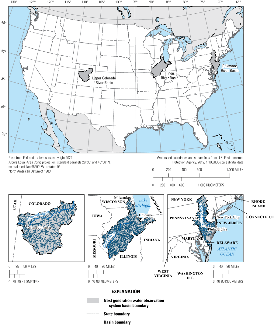
Map showing the location of the three hydrologic basins: Delaware River Basin, Illinois River Basin, and Upper Colorado River Basin.
Section I: Data Distribution by Element, Fraction and Hydrologic Basin
Retrieval of water-quality data from the WQP provide more than 1,500,000 unique observations for 3 fractions (filtered, unfiltered, and particulate) of the 12 elements under study, across all 3 hydrologic basins (DRB, ILRB, and UCOL) and over a 120-year time period (1900–2022) (Marvin-DiPasquale and others, 2022). However, given the diversity of Federal, State, and local/municipal agencies that contribute to this immense data repository; the mix of historical, provisional, and final/accepted data results; the variation in analytical methods used and associated DQLs for any given element; and the variation in the level of reporting detail provided by the submitting laboratory or agency, it is not surprising that a significant amount of data screening and preliminary analysis is needed before various subsets of the retrieved data can be used for eventual spatial and temporal modeling.
The first assessment is a summary of the overall distribution of sample counts associated with the data retrieved (as published in Marvin-DiPasquale and others, 2022) by element, fraction, and basin (table 1). Of the 3 hydrologic basins, the ILRB yielded the most observations (n=641,118), followed by the UCOL (n=548,199) and the DRB (n=338,511). These observation totals include cases where a sample was collected but no result was reported, typically because the measured value was below the given DQL. Across all basins, the element with the least observations was uranium (n=3,599), followed by mercury (n=40,936). Iron yielded the highest number of observations for the ILRB (n=75,037) and the UCOL (n=72,637), whereas copper had the highest number of observations in the DRB (n=49,108). An outcome of this assessment was that, across individual elements and basins, the relative number of observations associated with the particulate fraction was small (less than [<] 3.6 percent) compared with the filtered fraction (range from 11 to 77 percent) and unfiltered fraction (range from 23 to 88 percent). For all elements and basins (based on grand totals), these percentages were: 47.6 percent, 0.7 percent, and 51.7 percent for the filtered, particulate, and unfiltered fractions, respectively. The implication for developing viable spatial or temporal models is that the most data-rich models would be those that focused on the filtered and (or) unfiltered fraction data.
Table 1.
Summary of total observations by element, fraction, and basin (Delaware River, Illinois River, and Upper Colorado River), 1900–2022.[The data presented represent a sample count summary of all (1900–2022) surface water elemental concentration data retrieved from the Water Quality Portal, as reported in Marvin-DiPasquale and others (2022). The total sample count for each basin/element/fraction data grouping includes situations where no result value was reported, although a sample was collected. A hyphen (—) indicates that no samples were collected for that basin/element/fraction data grouping. n, number of observations; %, percentage; Filt., filtered fraction; Part., particulate fraction; Unfilt., unfiltered fraction]
Section II: Analytical Methods and Detection Quantitation Limits
The next assessment of the data retrieved from the WQP is an examination of the range of methods used to analyze each of the 12 elements. To the extent that method information reported in the WQP was available, the data coding for analytical methods used was harmonized (made consistent) in the initial data release (Marvin-DiPasquale and others, 2022) in the column titled “ADDED_Method_Info.” The original WQP metadata that informed this method harmonization and coding step included that from the following four columns: “ResultAnalyticalMethod.MethodIdentifier,” “ResultAnalyticalMethod.MethodIdentifierContext,” “ResultAnalyticalMethod.MethodName,” and “MethodDescriptionText.” The authors ultimately identified and coded for 23 method categories. For the purposes of the data analysis presented in this report, we further combined and harmonized the list of methods into 13 categories (table 2, refer to the footnote in table 2) and did not include analyses performed on the particulate fraction, given its low proportion of the total dataset (refer to Section I). Instead, the analysis of methods was done by combining the results for the filtered and unfiltered surface water fractions for each element.
For the complete 1900–2023 dataset (excluding the particulate fraction), 31.1 percent of the entries did not report the methods used and were thus coded as method UNKNOWN (table 2). For specific elements, the percentage of the data coded as method UNKNOWN was as follows: Al, 26.4 percent; As, 16.0 percent; Cd, 34.1 percent; Cr, 45.0 percent; Cu, 30.3 percent; Fe, 35.3 percent; Pb, 31.1 percent; Mn, 35.4 percent; Hg, 52.0 percent; Se, 12.9 percent; U, 24.3 percent; and Zn, 30.3 percent. Based on methods data that were reported, inductively coupled plasma-optical emission spectrometry (ICP-OES) was the most common method used to analyze for Al, Cd, Cr, Cu, Fe, Mn, Pb, and Zn. Inductively coupled plasma-mass spectrometry (ICP-MS) was the most commonly reported method for As and Se, although the number of reports of analysis by ICP-MS and ICP-OES were comparable for As, Se and Pb. In contrast, ICP-MS was the dominant method for analyzing U. Cold vapor atomic absorbance spectrometry (CVAAS) was the dominant method for analyzing Hg, followed by cold vapor atomic fluorescence spectrometry (CVAFS).
Table 2.
Summary of analytical methods, by element.[Values represent the number of observations (n) and the percentage (%) of method types, by element, reported in Marvin-DiPasquale and others (2022). Method categories were further harmonized from those reported in the original data release.1 This analysis excludes methods associated with the particulate fraction. Harmonized method codes are as follows: AAS, atomic absorption spectrometry; ASPEC, alpha spectrometry-chemical separation; COLOR, colorimetry; CVAAS, cold vapor atomic absorption spectrometry; CVAFS, cold vapor atomic fluorescence spectrometry; FLUOR, fluorometry; HGAAS, hydride generation atomic absorption spectrometry; ICP-MS, inductively coupled plasma-mass spectrometry; ICP-OES, inductively coupled plasma-optical emission spectrometry; NCOUNT, delayed-neutron counting; PHOS, phosphorimetry (laser) phosphorescence; POT, potential dissolved metals. The method code UNKNOWN indicates insufficient method information was provided from the original data source.]
There were 23 method codes presented in the harmonized data column “ADDED_Method_Info” in the original data report (Marvin-DiPasquale and others, 2022). An additional round of code harmonizing and condensing was performed for the data summary presented here. Methods codes in the original report were further condensed as such: atomic absorption spectrometry (AAS) [includes AAS, AAS-Dig, AAS-ext, and GFAAS], FLUOR [includes FLUOR, FLUOR-dir, and FLUOR-ext], IPC-MS [includes ICP-MS, and cICP-MS], ICP-OES [includes ICP-OES, DCP-AES, DCP-AES-dig, and ICP-AES], and UNKNOWN [includes NA and Unknown Method]. See Marvin-DiPasquale and others (2022) for additional definitions of these harmonized method codes.
Before the 1970s, the total number of observations in the retrieved dataset was scant, with fewer than 40 observations for any given element between 1900 and 1969. It was not until the 1970s that any single element exceeded 1,000 measurements. Furthermore, no specific method information was provided for any of the data entries before 1970. Figure 2 illustrates the temporal change in the total number of elemental concentration data observations (excluding the particulate fraction data) retrieved from the WQP (Marvin-DiPasquale and others, 2022) since 1970 in decadal time steps (except for 2010–22). For 11 of the 12 elements, there was either a substantial increase or a comparable count in the total number of observations (n) in the database, with each successive period. The one exception to this trend was for Hg, for which n decreased nearly 50 percent between the 2000–09 and 2010–22 periods. Similarly, the percentages for the reporting of the methods used and the DQLs generally increased over time. For the complete 1970–2022 time period, 31 percent of all data entries (excluding the particulate fraction) did not report a method and 40 percent did not report a DQL. However, by 2010–22, most elements (except for Hg and U) had more than 90 percent of the entries clearly identifying the methods used and 9 out of 12 had more than 70 percent of the entries reporting DQL values (except for Fe, Mn, and Zn). Thus, although the reporting of methods and DQL information increased over time, this reporting was neither necessarily consistent across element nor tightly coupled.
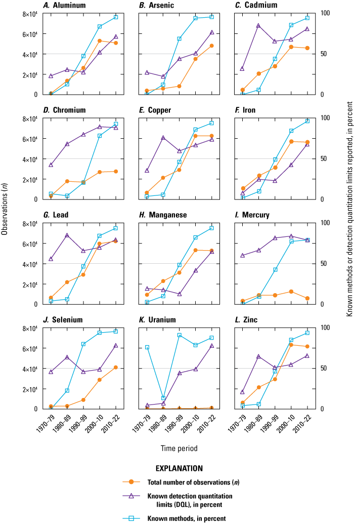
Time-series line plots showing the percentage of data for which specific methods and detection quantitation limits (DQLs) were identified for the 1970–79, 1980–89, 1990–99, 2000–10, and 2010–22 periods, by element. The left y-axis depicts the total number (n) of observations retrieved from the Water Quality Portal (excluding the particulate fraction). The right y-axis depicts the percentage (%) of the total values for which either methods or DQL information was reported. The data used for this plot are published in Marvin-DiPasquale and others (2022).
Based on the updated list of 13 method categories (table 2), summary statistics were calculated for the DQL data originally presented in Marvin-DiPasquale and others (2022) to examine the change in methods used and DQLs over time for specific elemental analyses. Summary statistics include the number of observations (n) of each method by decade (with the most recent temporal category as 2010–22) and the following statistics for all reported DQL data (by method, element, and period): mean, standard deviation, geometric mean, and quantiles (10th, 25th, 50th, 75th, and 90th). The complete statistical summary output for this analysis is available in DR_Table_1 (Marvin-DiPasquale and others, 2025). The decadal analysis of specific methods and associated DQLs excludes entries for which a DQL value was not reported. Of the more than 908,400 data entries for which DQL information was reported, 29.2 percent were coded as method UNKNOWN.
The graphical presentation of the total number of measurements with associated DQL data, by method, begins with the 1970s, when 6 of the 12 EoC (Cr, Cu, Fe, Pb, Mn, and Zn) were reported to have been analyzed using ICP-OES (fig. 3). During the 1970s, most analyses were for Pb (n=3,554), followed by Cu (n=2,339) and Hg (n=2,054). It was not until the 1980s that the total number of analyses exceeded 5,000 for half of the elements (Cd, Cr, Cu, Fe, Pb, and Hg) and the list of methods employed (with DQL values reported) expanded to include: AAS (for Al, Cd, Cr, Cu, Fe, Pb, Mn, and Zn), CVAAS (for Hg), HGAAS (for As and Se), ICP-OES (for Al, Cd, Cr, Cu, Fe, Pb, Mn, and Zn), and PHOS (for U). In the 1990s, this list was expanded to include ICP-MS for the analysis of Al, As, Cd, Cr, Cu Pb, Mn Se, U, and Zn. In the 1980s and 1990s, the number of samples reported with associated DQL values exceeded 5,000 for most of the 12 EoC (except for As, Mn, Se, and U, and Al during the 1980s). It was not until the 2000–09 period that CVAFS first appeared as a significant method for analyzing Hg and when all elements (except for U) exceeded 10,000 reported measurements. For the most recent period (2010–22), the number of measurements with reported DQLs exceeded 30,000 for all 12 EoC, except for Hg and U. Over the same 1970–2022 period, the number of WQP data entries that included DQL values but where the method was not identified (coded as UNKNOWN) decreased over time (fig. 3) as follows (as a percentage of all observations [n], by time period): 1970s (96.3 percent of n=17,705), 1980s (95.1 percent of n=101,743), 1990s (77.1 percent of n=117,395), 2000s (16.6 percent of n=290,617), and 2010–22 (3.1 percent of n=380,707).
The synopsis of results associated with the methods and DQL analysis are tabulated in DR_Table_1 (Marvin-DiPasquale and others, 2025) and are graphically presented in figures 2 and 3. The key results are: (a) a progressive increase over time in the number of specific methods employed and clearly identified between the 1970s and 2010–22 periods; (b) a more than 21-fold increase in the number of total analyses (from 17,705 to 380,707) where DQLs were reported over the same period; and (c) a striking decrease (from 96.3 to 3.1 percent) in the number of cases for which DQLs were reported but the actual method used was not over the same 52-year span.
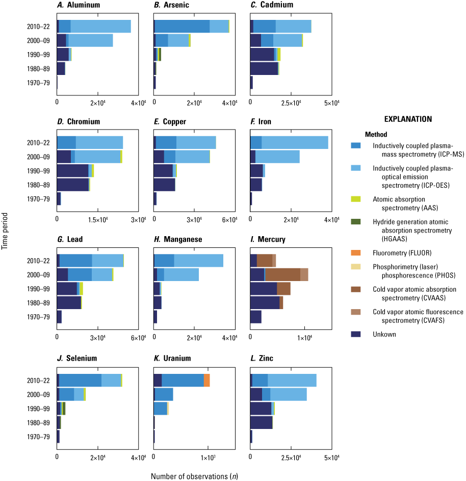
Horizontal stacked bar plot showing the number of retrieved WQP database observations (n), by method and time period, between 1970 and 2022. This data analysis includes results for filtered and unfiltered surface water samples (combined) and excludes particulate fraction analyses. The analysis further excludes any data entries that did not include a detection quantitation limit (DQL) value. For each panel, the x-axis was allowed to vary and was individually optimized to best allow for the visual discrimination of the various method categories. The primary data for this plot are published in Marvin-DiPasquale and others (2022), with the detailed statistical analysis summarized in DR_Table_1 (Marvin-DiPasquale and others, 2025).
Median DQL values, by element, method (excluding the UNKNOWN methods category), and time period (from 1970 to 2022), are graphically presented in figure 4. Although the individual plots depict substantial variation in the data, several observations are offered. First, the absolute range (from minimum to maximum, regardless of method) in median DQLs for crustal elements like Al and Fe (both 1–50 micrograms per liter [µg/L]) was substantially higher than for trace elements like Hg (0.01–0.10 µg/L) and U (0.05–1.0 µg/L). These differences reflect the relative abundance of the various elements in typical environmental surface water samples, driven by the need to develop and employ methods with appropriate DQLs that allow for the detection of environmentally relevant concentrations. Second, the relative range (maximum divided by minimum) of median DQLs for this same time period (independent of method) varied from tenfold for Hg (0.01–0.10 µg/L) and Cu (1–10 µg/L) to more than 1,000 fold for Pb (0.2–200 µg/L), with all other elements falling within this relative range of 10 to 1,000.
Finally, the apparent variation in median DQL values for any individual element (fig. 4) may reflect several factors, one of which is a shift over time in the dominant analytical approach(es), with differing DQLs being reported to the WQP. This could reflect overall changes in dominant analytical methods used by the scientific community or changes over time in the composition of the specific agencies (Federal, State, and local) performing field sampling programs of variable intensity, using various methods with variable DQLs, and reporting the results to the WQP database. In either case or in some combination, these types of analytical changes over time would be reflected in the variability seen in the median DQL results. For example, both As and Se exhibited a marked increase in the number of analyses being run by ICP-MS and ICP-OES since 1990 (fig. 3). However, the median DQL for As was fivefold to tenfold lower for ICP-MS (1–2 µg/L) compared with ICP-OES (10 µg/L). For Se, the median DQL was also significantly lower for ICP-MS (1 µg/L) compared with ICP-OES (7–20 µg/L) during the 1990–2009 period, but the same for both methods (5 µg/L) during the 2010–22 period (fig. 4). The apparent increase in the median DQL for Se using the ICP-MS method between the 1990–2009 and 2010–22 periods is reflective of data from various laboratories, with differing DQL values dominating the data provided to the WQP in subsequent periods, and not necessarily an actual increase in DQL over time from a single laboratory. A second example of the introduction of new method and its influence on reported DQL values over time can be seen in the case of Hg. Between 1980 and 1999, the single analytical method for Hg reported in the retrieved dataset was CVAAS, with a median DQL ranging from 0.06 to 0.1 µg/L. By the 2000s, reports of the use of CVAFS for Hg analysis began appearing, which is a method with a substantially lower median DQL (0.01 µg/L) compared with CVAAS (fig. 4).
Another factor that likely drives some of the observed trends in median DQL values over time is improvements in the development of and adherence to standardized laboratory and field sampling clean techniques and quality assurance protocols. A suggested example of these types of improvements may be the significant and permanent decrease in the DQL values associated with the ICP-OES analysis of Cr, Pb, and Zn after the 1970s (fig. 4).
A nonparametric Wilcoxon rank-sum statistical test was performed on the element-specific DQL decadal geomean values presented in DR_Table_1 (Marvin-DiPasquale and others, 2025) for all identified method categories and the UNKNOWN method category combined, with the reported geomean values binned into pre- and post-1990 temporal groupings. Five of the 12 elements had statistically significantly lower DQL values for the post-1990 grouping (Cd, Cr, Cu, Pb, and Hg). The remaining seven elements (Al, As, Fe, Mn, Se, U, and Zn) had no significant difference for the DQL decadal geomean values between the two temporal groupings.
Although a more detailed examination of the changes in analytical methods and DQL values associated with the EoC data originally retrieved from the WQP (Marvin-DiPasquale and others, 2022) is beyond the scope of this report, the statistical summary analysis performed on that data is presented in DR_Table_1 (Marvin-DiPasquale and others, 2025) and is available for additional investigation. Furthermore, the combination of more method-specific and DQL-specific information being reported to the WQP since the 1990s, along with lower DQL values observed for 5 of the 12 EoC since the 1990s, suggests that data collected before the 1990s may be of somewhat lesser value for future modeling efforts.
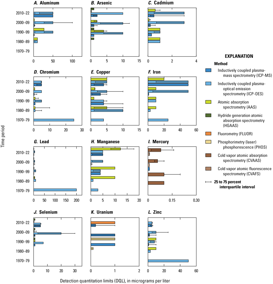
Horizontal bar plot showing median detection quantitation limit (DQL) values for the 12 EoC, by method and time period, between 1970 and 2022. DQL units are in micrograms per liter (µg/L). Error bars represent the 25 percent–75 percent interquartile interval. The data analysis includes results for filtered and unfiltered surface water samples (combined) and excludes particulate fraction data. The analysis further excludes any data entries that did not include a DQL value. For each panel, the x-axis was allowed to vary and was individually optimized to best allow for the visual discrimination of the various method categories. The primary data for this plot are published in Marvin-DiPasquale and others (2022), with the detailed statistical analysis summarized in DR_Table_1 (Marvin-DiPasquale and others, 2025).
Section III. Analysis of Censored Data
A critical step in the preparation and consideration of the surface water EoC concentration data retrieved from the WQP, as it pertains to potential modeling efforts, is an analysis of the extent and type of data censoring that exists in the dataset. In this context, “censored data” refers to any concentration result value that was either deemed to be above or below the laboratory’s established concentration range of acceptable results or was identified in some other way as being suspect or nonreportable. There were six types of result value data censoring that were identified in the EoC dataset published in Marvin-DiPasquale and others (2022), which were harmonized and categorized as: (a) left-censored with a negative value reported, (b) left-censored with a positive value reported, (c) left-censored with no value reported, (d) left-censored with a zero (0) value reported, (e) right-censored, and (f) censored for some other reason. The phrase “left-censored” indicates that the value was below the reporting laboratory’s DQL, whereas the phrase “right-censored” indicates that the value was above the reporting laboratory’s upper reporting limit. In addition to the above six categories of data censoring, the seventh category in the harmonization scheme employed was “not censored,” meaning that there was no form of data censoring and that the reported value was presumed to be valid and within the reporting limits for the laboratory submitting data to the WQP.
An analysis of data censoring, within the context of the above seven categories, was performed on the EoC concentration data originally published in Marvin-DiPasquale and others (2022) and summarized in DR_Table_2 (Marvin-DiPasquale and others, 2025). This analysis consisted of sample counts (and expressed as percentages) for each censoring category, subset by each basin/element/fraction data grouping for the complete 1900–2022 dataset, as well as for the period before 1990 (pre-1990) and the period after (and including) 1990 (post-1990). These additional pre- and post-1990 analyses were completed based on the lower percentages of methods and DQL values reported (fig. 2) and the statistically higher median DQL values for several elements in the pre-1990 period (refer to Section II), suggested that the pre-1990 data may be of lesser or questionable value for use in modeling compared with the post-1990 data.
The post-1990 period represented most (83 percent) of the complete 1900–2022 dataset. There was a notable decrease in the percentage of data that was censored (by using any censoring category) between the pre-1990 and post-1990 periods. Specifically, across all elements and basins, filtered samples decreased from 63 percent censored (pre-1990) to 55 percent censored (post-1990), particulate samples decreased from 31 percent censored (pre-1990) to 0.8 percent censored (post-1990), and unfiltered samples decreased from 54 percent censored (pre-1990) to 41 percent censored (post-1990). These results suggest that generally lower analytical detection limits in the post-1990 period across the suite of elements under consideration.
The comparison of censored versus noncensored data becomes more nuanced when broken down by the individual EoC. Figure 5 depicts the relative percentages of the censored (all censoring categories combined) and the noncensored data, by basin/element/fraction data groupings (excluding the particulate fraction) for the post-1990 period (only). In nearly all cases, the percentage of censored data was higher for filtered samples than for unfiltered samples. The one consistent exception was in the case of Se, where the percentage of censored data was consistently higher in the unfiltered samples, for all three hydrologic basins. The crustal elements Al and Fe also exhibited a lower percentage of censored values in the unfiltered fraction compared with the filtered fraction in the ILRB and the UCOL, but this difference was not as pronounced in the DRB. For the filtered fraction, the elements with the highest degree of censoring (greater than [>]75 percent), by basin, were as follows: Cd, Pb, and U for the DRB; Cd, Cr, Pb, Hg, and Se for the ILRB; and Cr, Pb, and Hg for the UCOL. For the unfiltered fraction, the elements with the highest degree of censoring (>75 percent), by basin, were as follows: Cd, Hg, and Se for the ILRB; and Hg for the UCOL. There were no elements in the DRB for which >75 percent of the unfiltered data was censored. For the filtered fraction, the elements that had the lowest percentage (<25 percent) of censored data, by basin, were as follows: Al, Fe, and Mn for the DRB; Mn and U for the ILRB; Mn only for the UCOL. For the unfiltered fraction, the elements that had the lowest percentage (<25 percent) of censored data, by basin, were as follows: Al, Fe, and Mn for the DRB; Al, Fe, Mn, and U for the ILRB; Al, Fe, and Mn for the UCOL. The observation that 100 percent of the U samples in the ILRB post-1990 dataset were noncensored is based upon the fact that there were only a few filtered (n=28) and unfiltered (n=36) samples in this grouping, none of which were censored. This is in comparison to the number of U samples in the post-1990 dataset in the DRB (n=321 filtered, n=1,484 unfiltered) and the UCOL (n=170 filtered, n=648 unfiltered), all which had a significant percentage of censored values.
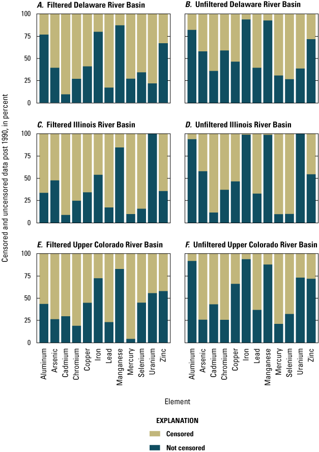
Stacked bar plots of the percentage of censored and noncensored data post-1990, by element, basin, and fraction (filtered and unfiltered). The primary data for this figure are published in Marvin-DiPasquale and others (2022), with the detailed statistical analysis summarized in DR_Table_2 (Marvin-DiPasquale and others, 2025). The censored category depicted in this figure represents the sum of all six censored data categories identified in Section III of this report and reported in the above two data releases.
Section IV: Median EoC Concentrations by Catchment
In preparation for modeling the spatial distribution of the 12 targeted EoC at the basin level, as a function of geospatial attributes, several preliminary data cleaning, and screening steps are required. The three overarching steps described are: (a) the calculation of median concentration values for each element/fraction at the catchment level; (b) the calculation of a single censoring value for each basin/element/fraction data grouping; and (c) the screening of these median concentration data groupings with respect to data density and distribution, and relative to established regulatory thresholds. This section covers the first two of these process steps, whereas Section V covers the third.
The geospatial data for the ongoing modeling effort are derived mostly from databases in the NHDPlus framework (U.S. Environmental Protection Agency, 2024), which provide geospatial attribute data at the catchment spatial scale. Thus, the first step in working with the published EoC concentration data (Marvin-DiPasquale and others, 2022) was to convert that site-specific point data to catchment scale data, after first removing all EoC concentration data collected before 1990. These calculations relate only to the 1990–2022 (post-1990) subset of the original WQP data retrieval. Furthermore, only filtered and unfiltered fraction data were considered in this workflow; particulate fraction data were not considered.
For the purpose of spatially aggregating the EoC concentration data, each discrete sampling location was identified within a NHDPlus defined catchment using ArcGIS Pro (version 3.0; Esri, 2022). Samples that were coded as “nondetect” and that also had no reported DQL were removed. Catchments with fewer than three data entries (per element/fraction data grouping) were also removed. No data were removed based on the specific analytical method used. Median concentration values were then calculated for each catchment/element/fraction data grouping by using the Kaplan-Meier statistical approach (Helsel, 2010), which estimates median values more accurately when some values may be censored and determines if the calculated median itself is censored. All calculations associated with the catchment medians were performed in R (version 4.3.2; R Core Team, 2024). Further details for these preparatory data steps are described in the metadata section of the companion data release for this report, along with the tabular data associated with the median concentration values for each catchment/element/fraction data grouping, as presented in DR_Table_3 (Marvin-DiPasquale and others, 2025). A graphical example of what these median catchment results look like spatially is given for filtered arsenic in all three hydrologic basins (fig. 6).
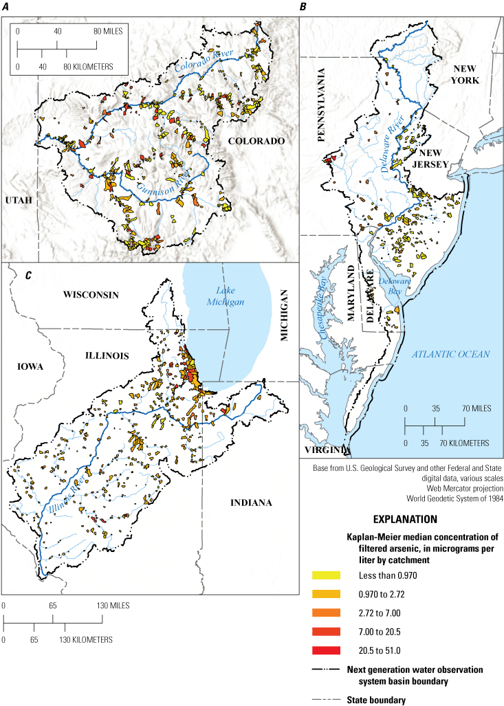
Maps depicting the calculated median concentrations of filtered arsenic in surface water at the catchment scale for the three hydrologic basins (Delaware River Basin, Illinois River Basin, and Upper Colorado River Basin). The data used in calculating these median concentration values are restricted to data collected during the 1990–2022 period, as reported in the WQP (Marvin-DiPasquale and others, 2022). Concentration units are in micrograms per liter (µg/L). The calculated medians for this figure are published in DR_Table_3 (Marvin-DiPasquale and others, 2025).
Given the variation in the degree of censored data associated with individual elements and fractions for the discrete measurements (refer to Section III), the calculated median concentrations also exhibited a high degree of variability with respect to censored values at the catchment scale. Specifically, before determining a single censoring value for each basin/element data grouping, the range in the percentage of catchments with censored median values was as follows for the 12 EoC (combining all basins and both fractions): Al, 0.2–33.0 percent; As, 21.6–41.8 percent; Cd, 30.6–80.7 percent; Cr, 26.3–86.9 percent; Cu, 17.2–47.6 percent; Fe, 0.2–9.2 percent; Pb, 20.8–68.2 percent; Mn, 0–5.7 percent; Hg, 44.8–94.5 percent; Se, 31.6–88.6 percent; U, 0–72.2 percent; Zn, 11.8–29.6 percent. The detailed tabular results of this assessment can be found in DR_Table_4 (Marvin-DiPasquale and others, 2025).
The machine learning modeling approach being pursued deciphers which geospatial attributes (not presented herein) are most strongly correlated with the basin-scale spatial distribution of EoC concentrations requires a single censoring value for each data grouping. Thus, each grouping was recensored to a single value by first assessing upper-end outlier median DQL catchment values (those exceeding the 95-percent quantile) and then defining the highest censoring value that was not an outlier as the single censoring value for that basin/element/fraction grouping. The upper-end outlier values were removed for the purposes of modeling. Further details of this recensoring process and the tabulated results can be found in DR_Table_4 (Marvin-DiPasquale and others, 2025). The final range in the percentage of catchments with censored median values for the 12 EoC (combining all basins and both fractions) was: Al, 10.6–99.6 percent; As, 98.2–100 percent; Cd, 92.7–100 percent; Cr, 99.6–100 percent; Cu, 91.8–100 percent; Fe, 0.2–89.8 percent; Pb, 60.2–100 percent; Mn, 0–74.5 percent; Hg, 99.5–100 percent; Se, 67.5–100 percent; U, 0–100 percent; Zn, 79.4–99.5 percent. Thus, recensoring each data grouping to a single censoring value significantly increased the percentage of catchments with censored median values. This step reflects that for each grouping, the single recensoring value is ultimately the highest nonoutlier censoring value from among all the individual catchments that had censored medians. One consequence of this machine learning approach and the necessity of recensoring to a single value (per element/fraction/basin) is associated with catchments that had concentration medians below the recensoring value, but not originally censored themselves. For these catchments, their median values are reassigned at the single recensoring limit, flipping their condition from not previously censored to censored.
Section V: Decision Tree for Geospatial—Machine Learning Models
There are a total of 72 geospatial models possible by using the 12 elements of concern, 2 fractions (filtered and unfiltered), and 3 hydrological basins. Each of these basin/element/fraction data groupings were screened for their potential to be further pursued with a machine learning modeling approach applied to geospatial attributes as explanatory variables. A decision tree (fig. 7) was constructed for this screening process. The decision tree has 5 steps (STEP A, B, C1, C2, and D) and 5 potential outcomes (model Categories 1, 2, 3, 4, and 5) (table 3). Each step poses a “yes/no” question of the data. A detailed tabular summary of the answers for each step and the resulting category code for all 72 potential models can be found in DR_Table_5 (Marvin-DiPasquale and others, 2025).
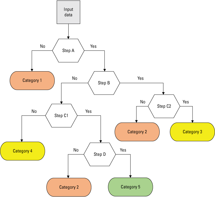
Graphical illustration of the decision tree. This decision tree is used to screen the 72 basin/element/fraction data groupings under consideration for their suitability to be modeled by using a machine learning approach applied to geospatial attributes as explanatory variables. See table 3 for the definitions of the five steps (A, B, C1, C2, and D) and five model categories (1, 2, 3, 4, and 5) depicted in this figure.
Table 3.
Decision tree STEPS and categories.[This table is associated with the illustration of the decision tree shown in figure 7 and provides the definitions of the five STEPS (A, B, C1, C2, and D) and five resulting model categories (1, 2, 3, 4, and 5) depicted on that figure. The input data are the catchment specific median elements of concern concentrations for each of the 72 potential basin/element/fraction data groupings, after a single censoring value has been defined for that specific data grouping. The catchment median values and the recensoring values are provided in DR_Table_3 and DR_Table_4 (Marvin-DiPasquale and others, 2025). %, percent]
The input data for the decision tree are the median catchment values for each basin/element/fraction grouping, as detailed in DR_Table_3 (Marvin-DiPasquale and others, 2025) after applying the single recensoring value described in Section IV and summarizing the final number of catchments and the percentage of censored catchments for that grouping, as detailed in DR_Table_4 (Marvin-DiPasquale and others, 2025).
For data groupings with less than 30 percent of catchment medians censored, and beginning with STEP C1, the decision tree considers the data in the context of regulatory threshold concentrations. Specifically, table 4 summarizes three categories of EPA regulatory thresholds, which are based on: (a) drinking water guidelines and standards, (b) human health criteria (HHC) standards, and (c) aquatic life criteria (ALC) standards (with acute and chronic thresholds). Although there are drinking water standards for all 12 EoC under consideration, only 5 elements have HHC thresholds (As, Cu, Mn, Se, and Zn) and only 6 elements have ALC thresholds (As, Cd, Hg, Fe, Pb, and Zn).
Table 4.
U.S. Environmental Protection Agency regulatory concentration thresholds for 12 elements of concern.[The table provides three general categories of U.S. Environmental Protection Agency (EPA) regulatory concentration thresholds for the 12 elements under study, including: (a) based on drinking water (DW) guidelines and standards from EPA (2009); (b) based on the recommended water quality “human health criteria” (HHC) from EPA (2023), which is given in terms of the consumption of both water and organisms or the consumption of organisms only; and (c) based on the freshwater aquatic life criteria (ALC), with both acute and chronic values given from EPA (2022). Concentrations are given for either dissolved (filter passing) or total (unfiltered) water, as appropriate, and in units of micrograms per liter (µg/L). An em dash (—) indicates that no regulatory threshold exists for that element/fraction data grouping. See footnotes for additional information.]
Source: National Primary Drinking Water Regulation Table (EPA, 2009).
Based on the ”Treatment Technique,” a required process intended to reduce the level of a contaminant in drinking water.
Source: National Recommended Water Quality Criteria—Human Health Criteria Table (EPA, 2023)
Source: National Recommended Water Quality Criteria—Aquatic Life Criteria Table (EPA, 2022)
Of the 72 basin/element/fraction data groupings run through the decision tree (fig. 7, table 3), 14 groupings (19.4 percent) were categorized as Category 1 (“Do not model” because of too few catchments) at STEP A. Of the remaining 58 groupings, only 7 (9.7 percent of the original 72) were found to have less than 30 percent censored data at STEP B and were thus shunted to STEP C1. Of the remaining 51 groupings, which had more than 30 percent censored data at STEP B and were thus shunted to STEP C2, 5 groupings (6.9 percent of the original 72) had between 30 and 70 percent censored data and were thus designated as Category 3 (Classification model based on detected or not-detected; LOW PRIORITY). The remaining 46 groupings (63.9 percent of the original 72) that were shunted to Step C2 had more than 70 percent censored data and were designated as Category 2 (Do not model; data are too imbalanced). The complete breakdown of the decision tree results for each of the 72 basin/element/fraction data groupings are presented in DR_Table_5 (Marvin-DiPasquale and others, 2025).
Of the 7 original 72 basin/element/fraction data groupings that were shunted to STEP C1, which focuses on groupings with less than 30 percent censored catchments and elemental concentrations assessed relative to specific EPA water quality thresholds (table 4), none of the groupings had all catchment median concentration data below the relevant EPA threshold. Thus, none of the 7 groupings that were assessed at STEP C1 were designated as Category 4 (Classification model based on a value below the regulatory value of interest; LOW PRIORITY) and all 7 groupings were assessed at STEP D. The decision tree results for this last step varied depending on the EPA threshold in question. Although all the decision tree results are fully detailed in DR_Table_5 (Marvin-DiPasquale and others, 2025), a summary of results for Categories 3 and 5 are provided in table 5.
Table 5.
Summary of decision tree results for model Categories 3 and 5.[This table represents a summary of a subset (Category 3 and 5 only) of the results more fully detailed in DR_Table_3, DR_Table_4, and DR_Table_5 (Marvin-DiPasquale and others, 2025), which documents the results of the decision tree analysis (fig. 7, table 3) of the 72 basin/element/fraction data groupings with respect to model categorization. The relevant U.S. Environmental Protection Agency (EPA) criteria, associated with Category 5 models, include those associated with drinking water (DW) and the human health criteria (HHC, organisms only), as per table 4. Criteria threshold values are given in micrograms per liter (µg/L). EPA criteria information is not applicable (NA) for Category 3 models based on the Decision Tree design. DRB, Delaware River Basin; ILRB, Illinois River Basin; UCOL, Upper Colorado River Basin]
Percentages after the recensoring, as derived from DR_Table_4 (Marvin-DiPasquale and others, 2025).
Calculated from the data in DR_Table_3 (Marvin-DiPasquale and others, 2025).
Given the 72 initial basin/element/fraction data groupings and up to five EPA criteria per element/fraction category (for example, Zn, table 4), the EoC data originally compiled from the WQP (Marvin-DiPasquale and others, 2022) resulted in 132 potential models that could be examined by using the geospatial machine learning approach that is being considered as part of the USGS Proxies Project (USGS, 2023a). The purpose of the decision tree exercise was to rigorously consider all these potential models with respect to data density, the extent of censored data, and the relevance to specific EPA water quality concentration thresholds for the 12 EoC. This aimed to limit the number of models under consideration to those that are most viable and environmentally relevant. Table 5 reflects this final list of models for further consideration.
In all, there are 6 models that are considered high priority (Category 5) to the extent that the percentage of censored catchments was less than 30 percent and that the number of catchments was reasonably well balanced (30–70 percent or 50 plus or minus [±] 20 percent) with respect to values above or below the EPA criteria under consideration (table 5). This type of data distribution lends itself most favorably to a categorical (above versus below EPA threshold) machine learning approach that could be coupled with geospatial attribute data to explain the spatial distribution of the observed catchment median EoC concentrations. These 6 models were limited to 3 elements (Al, Mn, and Fe), all which are found at comparatively high concentrations in surface waters relative to the other 9 EoC under study. Five of the 6 models were relative to EPA National Secondary Drinking Water Regulations, which are nonenforceable, and 1 (ILRB/Mn/unfiltered grouping) was related to the EPA HHC (organisms only) guideline (tables 4 and 5).
There are five models that are considered low priority (Category 3) since 30–70 percent of the catchments in the data groupings are censored. Given this degree of censoring, these groupings could lead to viable categorical (detect versus nondetect) geospatial machine learning models but were not further considered with respect to specific EPA threshold concentrations. These five models also included Al, Mn, and Fe, in addition to Pb and Se (table 5).
Section VI: Analysis of EoC Concentration Data at USGS Real-Time Sites
Fixed site time-series models represent a second model type that the existing EoC concentration data retrieved from the WQP (Marvin-DiPasquale and others, 2022) may readily lend themselves to. These models leverage continuous discharge and (or) water-quality sensor data from USGS monitoring sites as the explanatory variables used to estimate elemental concentrations or loads. For example, Mast (2018) developed a suite of surface water models (for filtered and unfiltered fractions) that estimated concentrations for 8 target elements (Al, As, Cd, Cu, Fe, Pb, Mn, and Zn) based on stream discharge and water-quality data (specific conductance, pH, turbidity, and water temperature) at 9 sites in the Animas and San Juan Rivers in Colorado. A few such models have also been developed at USGS real-time monitoring sites that provide computed continuous concentrations estimates for target elements, including: for As at 2 sites in Kansas (USGS, 2024d); for As and antimony (Sb) at 4 sites in Idaho (Baldwin and Etheridge, 2019; USGS, 2024b, c); and for Se estimated from specific conductance at 9 sites in Colorado (Linard and Schaffrath, 2014; USGS, 2024a).
The purpose of this preliminary assessment of the EoC concentration data initially retrieved from the WQP data (Marvin-DiPasquale and others, 2022) is to: (a) determine which subset of sampling locations constitute USGS continuous monitoring sites; (b) determine for each site which continuous discharge measurements and (or) sensor data were being collected during the period when discrete sampling occurred for the various element/fraction data groupings; (c) determine the number of discrete element/fraction samples collected at each site and what percentage of these were censored; and (d) determine what percentage of the EoC concentration data exceeded the various EPA threshold values given in table 4. The overarching goal of this assessment is to identify all site/element/fraction data groupings where there are enough noncensored data, which are environmentally relevant with respect to EPA thresholds, to justify pursuing time-series models that could potentially provide continuous EoC concentration or load estimates.
Of the 9,856 unique sites in the original WQP data retrieval, 4,480 (45 percent) were USGS surface water sites, with the remainder being non-USGS sites. Of the USGS sites, 285 sites also had continuous discharge measurement and (or) sensor data that overlapped in time with when discrete EoC data were collected. Once this subset of USGS sites with continuous data was identified, the date-time stamp of the discrete EoC data was matched (within the closest 15 minutes) to the site-specific continuous data, and the two datasets were merged into an initial dataset that consisted of site-specific discrete EoC concentration data and date-time matched discharge and (or) sensor data. The following seven types of continuous data were targeted: discharge, temperature, specific conductance, dissolved oxygen, pH, turbidity, and fluorescent dissolved organic matter.
After the initial merging of the discrete EoC concentration data with the discharge and (or) sensor data, the following three criteria were employed to remove individual site/element/fraction data groupings that were deemed to be of low quality with respect to data density, the percentage of censored data, and (or) environmental relevance, as follows:
-
• Data groupings with fewer than 50 EoC measurements were eliminated.
-
• Data groupings with greater than 25 percent censored data were eliminated.
-
• Data groupings for which less than 10 percent of the specific element concentrations were above any of the EPA threshold concentrations given in table 4 were eliminated.
The final resulting dataset of merged EoC concentration data and real-time site data, after screening by the above criteria, is published as DR_Table_6 (Marvin-DiPasquale and others, 2025). A data table derived from the information compiled in DR_Table_6 was then constructed in DR_Table_7 (Marvin-DiPasquale and others, 2025), which summarizes: (a) the number of EoC results for each site/element/fraction data groupings, (b) the number and percentage of censored EoC results for each data groupings, (c) the number of paired sensors values for each data grouping, and (d) which EPA criteria was exceeded for each data grouping. A coding column (Initial model variables) was added to DR_Table_7 that lists which of the seven types of continuous data were available for each site/element/fraction data grouping, after excluding those continuous data types with fewer than 50 observations.
Each site/element/fraction data grouping given in DR_Table_7 (Marvin-DiPasquale and others, 2025) thus represents a potential time-series model that could be further explored. Based on the data exclusion criteria described above, there were 177 data groupings at a total of 69 unique USGS continuous monitoring sites. Of the 177 data groupings, 163 (92 percent) had discharge as the only continuous monitoring variable, whereas the remaining 14 had 2 or more potential modeling variables (table 6). Unlike the analysis performed for the geospatial machine learning models, which included data collected since 1990, this final merged dataset from USGS real-time sites retained data as far back as 1981, as the provenance of the elemental concentration data was well known (all from the USGS) and well documented with respect to the methods used and the DQLs reported. The 1981–89 period represented 10.1 percent of all the observations in DR_Table_6 (Marvin-DiPasquale and others, 2025).
Table 6.
Summary of potential EoC time-series models at USGS continuous monitoring sites.[This table is a subset of DR_Table_7 given in Marvin-DiPasquale and others (2025) and excludes site/element/fraction data groupings (the model Y variable) with only one potential explanatory variable (the model X variable). EPA, U.S. Environmental Protection Agency; DW, drinking water (guideline or standard); HHC, human health criteria; flow, stream discharge; SC, specific conductance; Temp, temperature; DO, dissolved oxygen; Turb, turbidity; HHC, human health criteria; DW, drinking water (guideline or standard)]
The model screening results (table 6) lead to several conclusions related to the potential for further EoC time-series model development at USGS continuous monitoring sites. For models with more than one potential explanatory variable, there were: 5 final models at 3 unique sites within the DRB that included 3 elements (As, Fe, and Mn); 8 final models at 4 unique sites within the UCOL that included the same 3 elements (As, Fe, and Mn); and only 1 final model for 1 site within the ILRB, which was for As. Thus, out of the 12 EoC that made up the initial list, only 3 (As, Fe, and Mn) had sufficient data density (n>50) paired with at least 2 in situ continuous monitoring properties and a low enough percentage of censored EoC measurements (<25 percent) to be considered “high priority” with respect to furthering modeling efforts. This <25 percent censoring level criterion was selected based upon a study of data substitution methods that are most appropriate given the extent of data censoring (Antweiler, 2015). That study concluded a simple data substitution approach () is appropriate for datasets with less than 25 percent censored data. It was determined that applying this screening level to our final model list made the most sense given the many hundreds of initial potential models (unique site/element/fraction data groupings) associated with USGS real-time monitoring sites and the complexities involved with more advanced substitution methods for datasets with >25 percent censored data.
Of the 3 elements that made the final list given in table 6, Fe and Mn were identified as exceeding the drinking water standard (table 4) for more than 10 percent of the measurements in each data grouping, whereas As was identified as exceeding the human health criteria (table 4) at 1 site in each of the three hydrologic basins. The EPA HHC for As is particularly low (0.018 µg/L when consuming both water and organisms and 0.14 µg/L when consuming organisms only) compared to other elemental thresholds given in table 4, owing to the known carcinogenic effects of this element (U.S. Environmental Protection Agency [EPA], 2023). While the HHC for As is based on unfiltered water samples (table 4), the data associated with the three As models identified in table 6 was for filtered surface water samples. However, it stands to reason that if unfiltered water samples had been collected, those samples would have exceeded that same EPA HHC threshold for As.
Section VII: Ongoing Modeling Efforts
The currently underway spatial modeling effort involves a machine learning (random forest) analysis of hundreds of possible geospatial attributes (not presented herein) obtained from multiple geospatial data sources. These attributes may be broadly classified as those associated with climate, ecoregion, hydrology, landscape type, lithology, mining, population, soil, topography, and wildfire. The goal of this analysis is to identify those geospatial attributes that most strongly correlate with the observed basin-scale distribution of catchment median EoC concentrations (for example, fig. 6). In this model formulation, the EoC catchment median concentration data are considered the dependent variables, and the geospatial attributes are the independent (explanatory) variables. Individual catchment median values are categorized as being either above or below the relevant EPA threshold of concern to facilitate a “classification” style machine learning modeling approach. Thus, for catchments within a study basin where no data currently exist, the resulting list of the most significant model-predicted geospatial attributes may be used to assess if those catchments are likely to have EoC concentrations above or below the relevant EPA threshold.
There are several limitations to the machine learning type spatial models as envisioned and described above. The first limitation is related to data density. Analysis of the complete 1900–2022 dataset, with respect to the evolution of methods used, DQLs by method, data censoring, and the extent to which methods and DQLs were reported, led to the conclusion that data collected before 1990 (17 percent of the full 1900–2022 dataset) should be excluded from these machine learning models. Furthermore, since the geospatial attributes being considered are provided at the catchment spatial scale, it was necessary to similarly condense the original site-specific point data to the catchment scale. Thus, although any given catchment may have contained dozens or hundreds of discrete observations for a given metal/fraction, the calculation of a single median value per catchment resulted in a significant decrease in the number of observations within a given study basin for any given metal/fraction data grouping.
The second limitation in assessing the spatial trends and geospatial correlates of EoC concentrations at the basin scale is associated with data censoring constraints. This classification model machine learning approach necessitates that only a single censoring value be used for any given basin/element/fraction grouping. Thus, the recensoring of each basin/element/fraction data grouping to a single censoring value further limits the data resolution by forcing catchment medians with values lower than the single basin-wide recensoring value to be reclassified as left-censored (and recoded with the recensoring value) when their values before the recensoring step were not actually censored.
A third limitation of the spatial model assessment also results from the need to work with catchment medians, as opposed to the original discrete site-specific concentration data. The calculation of catchment median concentration values precludes any refined temporal analysis of the data, as these medians reflect a single value over the whole 1990–2022 period under consideration. However, given the magnitude, complexity, and diversity of the initial dataset, with respect to the when and at what frequency discrete samples were collected within a given catchment, it was concluded that further temporal considerations were beyond the scope of what is practical in the context of the primary goal, which is a better understanding of the spatial distribution of the data based on geospatial explanatory variables.
The approach to developing temporal models at discrete USGS real-time monitoring sites differs from that used for “spatial” models, as the temporal models do not utilize machine learning but instead use stepwise regression to develop empirical multivariable regression equations. The approach competes all possible combinations of a few potential explanatory variables to arrive at a top model. As opposed to the hundreds of potential geospatial explanatory variables used for the spatial models, the temporal models rely solely on seven potential in situ continuous measurements (discharge, pH, specific conductance, temperature, dissolved oxygen, turbidity, and (or) fluorescent dissolved organic matter) to the extent available at a given USGS monitoring site. In addition to these 7 primary X-variables, 4 data transformations of each are calculated , giving a total of as many as 35 potential explanatory variables as the starting point for the competitive stepwise regression analysis. Top model selection involves balancing the desire to minimize unexplained error by selecting the highest adjusted-R2 (coefficient of determination) with the desire to have the most parsimonious final model (that with the fewest model terms necessary). In addition, criteria imposed upon the top model selection process include: (a) verifying that all model terms, including the intercept, are significant at p-value [p]<0.05 (the probability of committing a Type II error); (b) verifying that individual model terms are not correlated (for example, correlation coefficients among paired model terms is <0.7); and (c) ensuring that the top model is not overparameterized by limiting the number of model terms allowed to 1/20th the number of total model observations.
In contrast to the spatial models, which excluded pre-1990 data, the temporal models covered a slightly broader time period (1981–2022). The reasoning for the broader time period is because all of the data associated with the USGS real-time site models were collected and analyzed by the USGS and included more complete metadata information regarding methods and DQLs and because continuous monitoring data at the final subset of USGS sites date back to 1981.
Most of the potential temporal models identified were associated with exceedances of EPA drinking water guidelines or standards, as opposed to exceedances of HHC or ALC thresholds. This reflects the fact that not all the 12 elements under consideration had listed HHC or ALC thresholds, in addition to the fact that the drinking water thresholds were generally lower than the HHC or ALC thresholds, when these latter thresholds were listed. Furthermore, most (92 percent) of the potential temporal models had discharge only as the single continuous variable upon which to develop a model. Not surprisingly, a cursory exploration of best-fit models with flow as the only continuous variable suggests that a high degree of unexplained error, and multivariable models appear much more promising. This may limit how many of the potential temporal models listed in DR_Table_7 (Marvin-DiPasquale and others, 2025) will be sufficiently robust and useful for estimating continuous elemental concentrations at USGS continuous monitoring sites.
Summary
The report documents the methodical screening of the stream surface water concentration data (more than 1.5 million observations) for 12 target elements of concern (aluminum, arsenic, cadmium, chromium, copper, iron, mercury, manganese, lead, selenium, uranium, and zinc) in three hydrologic basins (Delaware River Basin, Illinois River Basin and Upper Colorado River Basin). This data screening exercise was focused on defining the subset of data that are most appropriate for use in the further development of two distinct model types, one spatial and one temporal, each with different goals and considerations with respect to data suitability. The ongoing spatial modeling focuses on a machine learning analysis of geospatial attributes that most strongly correlates with the distribution of these elemental concentrations at the basin scale. The temporal modeling focuses on a multivariable stepwise modeling approach to develop equations for generating high-resolution time-series estimates of elemental concentrations at specific U.S. Geological Survey continuous monitoring sites, based on available discharge and (or) in situ sensor data.
Elemental concentrations were assessed with respect to: (a) fraction type (filtered, particulate, unfiltered), (b) analytical methods, (c) detection quantitation limits, (d) the extent to which analytical methods and laboratory detection quantitation limits values were reported, and (e) the extent to which the elemental concentration data were censored in some way. It was concluded that data associated with the particulate fraction was too limited to use for either model type and that data collected before 1990 would be of limited value in developing the geospatial machine learning type models. Data collected since 1990 were subsequently used to calculate median concentration values at the hydrologic catchment spatial scale. A decision tree was used to assess the suitability of the catchment median concentration data for developing the geospatial machine learning models, with a high priority status given to data groupings that involved concentrations that exceed known U.S. Environmental Protection Agency thresholds for drinking water, human health and (or) aquatic life. Out of 72 unique basin/element/fraction data groupings considered, 5 were classified as low priority and 6 were classified as high priority. Except for one low-priority data grouping for Pb and another for Se, the final list of all viable data groupings consisted of only 3 elements (Al, Fe, and Mn), which are typically found to occur at higher concentrations compared with the 9 other elements under consideration.
For the fixed-site time-series models, 177 site/element/fraction data groupings, associated with 69 unique USGS continuous monitoring sites, passed the screening criteria, although most (92 percent) had discharge only as the single variable. Of the remaining 8 percent (14 data groupings with 2 or more variables), As, Fe, and Mn were the 3 elements from 8 unique monitoring sites that warrant further investigation, based on the selection criteria used (table 6).
It is yet to be determined how many or which of the unique data groupings that have been identified in this report as viable candidates for further modeling consideration will result in final models that are of high value and acceptably accurate. However, the data screening approach presented herein provides a framework that itself can be of value when considering similar geospatial machine learning models and (or) time series models for other constituents of interest.
Acknowledgments
Financial support for this effort was provided by the U.S. Geological Survey (USGS) Water Quality Processes program of the Water Mission Area. The authors would like to thank the project sponsor, Sandy Eberts; program managers Elena Nilsen and Lori Sprague; and the Water Resources Availability Portfolio (WRAP) manager, Mindi Dalton, for their support of this project. In addition, we thank Ronald Antweiler (USGS, retired) and Benjamin Linhoff (USGS) for their valuable review comments.
References Cited
Antweiler, R.C., and the Group Comparisons, 2015, Evaluation of statistical treatments of left-censored environmental data using coincident uncensored data sets. II. Group comparisons: Environmental Science & Technology, v. 49, no. 22, p. 13439–13446. [Also available at https://doi.org/10.1021/acs.est.5b02385.]
Baldwin, A.K., and Etheridge, A.B., 2019, Arsenic, antimony, mercury, and water temperature in streams near Stibnite mining area, central Idaho, 2011–17: U.S. Geological Survey Scientific Investigations Report 2019–5072, 20 p. [Also available at https://doi.org/10.3133/sir20195072.]
Helsel, D.R., 2010, Summing nondetects—Incorporating low-level contaminants in risk assessment: Integrated Environmental Assessment and Management, v. 6, no. 3, p. 361–366. [Also available at https://doi.org/10.1002/ieam.31.]
Linard, J.I., and Schaffrath, K.R., 2014, Regression models for estimating salinity and selenium concentrations at selected sites in the Upper Colorado River Basin, Colorado, 2009–2012: U.S. Geological Survey Open-File Report 2014–1015, 28 p. [Also available at https://doi.org/10.3133/ofr20141015.]
Marvin-DiPasquale, M., McCleskey, B.R., Sullivan, S.L., Ransom, K.M., Root, C., Kakouros, E., Kieu, L.H., and Agee, J.L., 2025, Select elements of concern in surface water of three hydrologic basins (Delaware River, Illinois River and Upper Colorado River)—Data screening for the development of spatial and temporal models: U.S. Geological Survey data release, https://doi.org/10.5066/P9M11AQX.
Marvin-DiPasquale, M.C., Sullivan, S.L., Platt, L.R., Gorsky, A., Agee, J.L., McCleskey, B.R., Kakouros, E., Walton-Day, K., Runkel, R.L., Morriss, M.C., Wakefield, B.F., and Bergamaschi, B., 2022, Concentration data for 12 elements of concern used in the development of surrogate models for estimating elemental concentrations in surface water of three hydrologic basins (Delaware River, Illinois River and Upper Colorado River): U.S. Geological Survey data release, https://doi.org/10.5066/P9L06M3G.
Marvin-DiPasquale, M.C., Sullivan, S.L., Soto-Perez, J., and Hansen, J., 2023, Concentration data for 12 elements of concern in surface water of three hydrologic basins (Delaware River, Illinois River and Upper Colorado River)—A data visualization tool: U.S. Geological Survey database, https://www.usgs.gov/tools/concentration-data-12-elements-concern-surface-water-three-hydrologic-basins-delaware-river.
Mast, M.A., 2018, Estimating metal concentrations with regression analysis and water-quality surrogates at nine sites on the Animas and San Juan Rivers, Colorado, New Mexico, and Utah: U.S. Geological Survey Scientific Investigations Report 2018–5116, 68 p. [Also available at https://doi.org/10.3133/sir20185116.]
R Core Team, 2024, R—A language and environment for statistical computing: R Foundation for Statistical Computing software release. [Also available at https://www.r-project.org/.]
U.S. Environmental Protection Agency [EPA], 2009, National primary drinking water regulation table, EPA 816–F–09–004: Washington, D.C., U.S. Environmental Protection Agency, 6 p., accessed April 24, 2024, at https://19january2017snapshot.epa.gov/ground-water-and-drinking-water/national-primary-drinking-water-regulation-table_.html.
U.S. Environmental Protection Agency [EPA], 2022, National recommended water quality criteria—Aquatic life criteria table: U.S. Environmental Protection Agency web page, accessed April 15, 2022, at https://www.epa.gov/wqc/national-recommended-water-quality-criteria-aquatic-life-criteria-table#a.
U.S. Environmental Protection Agency [EPA], 2023, National recommended water quality criteria—Human health criteria table: U.S. Environmental Protection Agency web page, accessed April 24, 2024, at https://www.epa.gov/wqc/national-recommended-water-quality-criteria-human-health-criteria-table.
U.S. Environmental Protection Agency [EPA], 2024, NHDPlus (National Hydrography Dataset Plus): U.S. Environmental Protection Agency web page, accessed May 2, 2025, at https://www.epa.gov/waterdata/nhdplus-national-hydrography-dataset-plus.
U.S. Geological Survey [USGS], 2021a, Next Generation Water Observing System (NGWOS): U.S. Geological Survey web page, accessed May 9, 2024, at https://www.usgs.gov/mission-areas/water-resources/science/next-generation-water-observing-system-ngwos.
U.S. Geological Survey [USGS], 2021b, NWIS Current Water Data for the Nation (real-time data): U.S. Geological Survey web page, accessed May 14, 2024, at https://www.usgs.gov/tools/nwis-current-water-data-nation-real-time-data.
U.S. Geological Survey [USGS], 2023a, Proxies Project: U.S. Geological Survey web page, accessed September 9, 2024, at https://www.usgs.gov/mission-areas/water-resources/science/proxies-project.
U.S. Geological Survey [USGS], 2023b, Integrated water availability assessments: U.S. Geological Survey web page, accessed May 9, 2024, at https://www.usgs.gov/mission-areas/water-resources/science/integrated-water-availability-assessments.
U.S. Geological Survey [USGS], 2024a, Colorado real-time water surrogates—Stations that measure or compute continuous selenium: U.S. Geological Survey database, accessed May 7, 2024, at https://nrtwq.usgs.gov/co/constituents/view/01145.
U.S. Geological Survey [USGS], 2024b, Idaho real-time water quality—Stations that measure or compute continuous antimony: U.S. Geological Survey database, accessed May 7, 2024, at https://nrtwq.usgs.gov/id/constituents/view/01095.
U.S. Geological Survey [USGS], 2024c, Idaho real-time water quality—Stations that measure or compute continuous arsenic: U.S. Geological Survey database, accessed May 7, 2024, at https://nrtwq.usgs.gov/id/constituents/view/01000.
U.S. Geological Survey [USGS], 2024d, Kansas real-time water quality—Stations that measure or compute continuous arsenic: U.S. Geological Survey database, accessed May 7, 2024, at https://nrtwq.usgs.gov/ks/constituents/view/01000.
Supplemental Information
Concentrations of chemical constituents in water are given in micrograms per liter (µg/L) or milligrams per liter (mg/L).
Abbreviations
ALC
aquatic life criteria
CVAAS
cold vapor atomic absorption spectrometry
CVAFS
cold vapor atomic fluorescence spectrometry
DQL
detection quantitation limit
DRB
Delaware River Basin
EoC
elements of concern
EPA
U.S. Environmental Protection Agency
HHC
human health criteria
ICP-MS
inductively coupled plasma-mass spectrometry
ICP-OES
inductively coupled plasma-optical emission spectrometry
ILRB
Illinois River Basin
n
number of observations
NHDPlus
National Hydrography Dataset Plus
UCOL
Upper Colorado River Basin
USGS
U.S. Geological Survey
WQP
Water Quality Portal
For more information about this report, contact:
Water Quality Processes Program Manager,
Oregon Water Science Center
U.S. Geological Survey
601 SW 2nd Ave, Suite 1950
Portland, OR 97204
or visit our website at
https://www.usgs.gov/centers/oregon-water-science-center
Publishing support provided by the Baltimore Publishing Service Center.
Disclaimers
Any use of trade, firm, or product names is for descriptive purposes only and does not imply endorsement by the U.S. Government.
Although this information product, for the most part, is in the public domain, it also may contain copyrighted materials as noted in the text. Permission to reproduce copyrighted items must be secured from the copyright owner.
Suggested Citation
Marvin-DiPasquale, M.C., McCleskey, R.B., Sullivan, S.L., Root, J.C., Seawolf, S.M., Ransom, K.M., Wherry, S.A., Kakouros, E., and Baesman, S., 2025, Select elements of concern in surface water of three hydrologic basins (Delaware River, Illinois River, and Upper Colorado River)—Data screening for the development of spatial and temporal models: U.S. Geological Survey Open-File Report 2025–1033, 25 p., https://doi.org/10.3133/ofr20251033.
ISSN: 2331-1258 (online)
Study Area
| Publication type | Report |
|---|---|
| Publication Subtype | USGS Numbered Series |
| Title | Select elements of concern in surface water of three hydrologic basins (Delaware River, Illinois River, and Upper Colorado River)—Data screening for the development of spatial and temporal models |
| Series title | Open-File Report |
| Series number | 2025-1033 |
| DOI | 10.3133/ofr20251033 |
| Publication Date | June 23, 2025 |
| Year Published | 2025 |
| Language | English |
| Publisher | U.S. Geological Survey |
| Publisher location | Reston, VA |
| Contributing office(s) | WMA - Earth System Processes Division |
| Description | Report: v, 25 p.; 2 Data Releases |
| Country | United States |
| State | Colorado, Delaware, Illinois, Indiana, Maryland, New Jersey, New York, Pennsylvania, Wisconsin |
| Other Geospatial | Dellaware River basin, Illinois River basin, Upper Colorado River basin |
| Online Only (Y/N) | Y |
| Additional Online Files (Y/N) | N |