

Water Supply in the Conterminous United States, Alaska, Hawaii, and Puerto Rico, Water Years 2010–20
Links
- Document: Report (54.4 MB pdf) , HTML , XML
- Larger Work: This publication is Chapter B of U.S. Geological Survey Integrated Water Availability Assessment—2010–20
- Data Release: USGS data release - Monthly ensemble outputs from the National Hydrologic Model Precipitation-Runoff Modeling System and the Weather Research and Forecasting model hydrologic modeling system for the conterminous United States, Alaska, Hawaii, and Puerto Rico for water years 2010–2020
- Version History: Version History (2 KB txt)
- NGMDB Index Page: version 1.0 (html)
- Download citation as: RIS | Dublin Core
Preface
This is one chapter in a multichapter report that assesses water availability in the United States for water years 2010–20. This work was conducted as part of the fulfillment of the mandates of Subtitle F of the Omnibus Public Land Management Act of 2009 (Public Law 111-11), also known as the SECURE Water Act. As such, this work examines the spatial and temporal distribution of water quantity and quality in surface water and groundwater, as related to human and ecosystem needs and as affected by human and natural influences. Chapter A (Stets and others, 2025a) introduces the National Integrated Water Availability Assessment and provides important background and definitions for how the report characterizes water availability and its components. Chapter A also presents the key findings of Chapters B–F and thus acts as a summary of the entire report. Chapter B (this report) is a national assessment of water supply, which is the quantity of water supplied through climatic inputs. Chapter C (Erickson and others, 2025) is a national assessment of water quality, which is the chemical and physical characteristics of water. Chapter D (Medalie and others, 2025) assesses water use including withdrawals and consumptive use in the conterminous United States. Chapter E (Scholl and others, 2025) presents an analysis of factors affecting future water availability under changing climate conditions. The National Integrated Water Availability Assessment culminates with Chapter F (Stets and others, 2025b), which is an integrated assessment of water availability that considers the amount and quality of water coupled with the suitability of that water for specific uses. Together, these six chapters constitute the National Integrated Water Availability Assessment for water years 2010–20.
Abstract
We present an assessment of water supply across the conterminous United States (CONUS), Alaska, Hawaii, and Puerto Rico covering water years 2010–20. Our analysis drew on two national hydrologic models, the National Hydrologic Model Precipitation-Runoff Modeling System and the Weather Research and Forecasting model hydrologic modeling system. Both models produced estimates of streamflow, evapotranspiration, soil moisture, snow water equivalent, and other hydrologic states and fluxes. The models were driven by the bias-adjusted 4-kilometer-resolution, long-term regional hydroclimate simulation over the conterminous United States dataset (CONUS404). We assessed spatial and temporal error distributions by comparing monthly simulations at the 12-digit hydrologic unit code and regional scale from both models against external benchmarking datasets. Results showed that average annual rainfall across the CONUS was 857 millimeters per year for the period of analysis, with water year 2012 the driest year (729 millimeters) and water year 2019 the wettest year (995 millimeters). Key interannual variability results included the following: (1) the California–Nevada hydrologic region had the highest variability in precipitation and snow accumulation, and (2) the Texas hydrologic region was among hydrologic regions with the highest variability in precipitation. We related interannual variability in precipitation to storage volumes in soil moisture, snow water equivalent, and lakes and reservoirs to highlight areas with little storage and large year-to-year variability in precipitation. These areas included the Southern High Plains, Central High Plains, Texas, Souris–Red–Rainy, Mississippi Embayment, and Midwest regions. Our analysis of groundwater-level data showed that several of these areas overlap aquifers where groundwater levels were considerably lower than historical averages, including the Colorado Plateaus aquifers, the Rio Grande aquifer system, and the Central and Southern regions of the High Plains aquifer. Many of these lowered groundwater levels are continuations of decades-long declines from overpumping that started well before the assessment period. The resulting water budgets and their analyses provide a high-resolution foundational assessment of the mean state and variability of the terrestrial hydrologic cycle across the CONUS and Alaska, Hawaii, and Puerto Rico to support a wide range of water resource management applications.
Key Points
The following are the key points of this chapter:
-
• Throughout much of the Great Plains and Northeast through Midwest aggregated hydrologic regions, low precipitation totals in water years 2011 and 2012 resulted in low streamflow, evapotranspiration, and soil moisture, associated with of the most substantial droughts since the 1930s.
-
• The highest interannual variability in precipitation was in the California–Nevada, Texas, Southern High Plains, and Southwest Desert hydrologic regions, whereas the lowest interannual variability was in the Florida, Tennessee–Missouri, and Northeast hydrologic regions.
-
• Among the Western aggregated hydrologic region, where snow is critical for water availability, the California–Nevada hydrologic region had the highest interannual variability in maximum snow accumulation with a coefficient of variation (CV) of 0.60, whereas the Columbia–Snake, Pacific Northwest, and Central Rockies hydrologic regions all had a CV of less than 0.36.
-
• Six of 29 unconfined and 6 of 23 confined principal and regional aquifer systems had current water-level percentiles (median 2010–20) of less than 30 percent of historical water levels (that is, median 2000–20 water levels) including the California Coastal Basin aquifers, the Colorado Plateaus aquifers, and the Central and Southern regions of the High Plains aquifer.
-
• Hydrologic regions with low precipitation and little storage coincide with aquifer systems that have shown a decline in groundwater levels during water years 2010–20, including the Southern High Plains, Central High Plains, and Texas hydrologic regions.
Introduction
Quantification of the mean state and variability of the current terrestrial hydrologic cycle is a fundamentally important part of understanding and describing water availability. The major reservoirs of the hydrologic cycle and the connections between them (hereinafter referred to as storage components and fluxes, respectively) are well understood (Abbott and others, 2019). Water evaporates from the surface of the ocean and land into the atmosphere where its movement is driven by wind. There it condenses to form precipitation, which falls to the Earth’s surface in the form of rain or snow. The fraction of precipitation that falls on land can be held temporally as snow or soil moisture or retained in lakes or reservoirs, or it can run off into streams and rivers, eventually discharging into the ocean. Some fraction of the precipitation that falls on land percolates more deeply to recharge groundwater in aquifers. The fraction of this cycle that occurs over or on the land’s surface is referred to as the terrestrial hydrologic cycle.
A comprehensive accounting of storage components and fluxes within the terrestrial hydrologic cycle is often referred to as a water budget, and the development of large, continental-scale water budgets has posed substantial challenges. Early efforts to develop quantitative budgets were limited by the availability and coverage of data (Nace, 1969). Later efforts such as the Global Energy and Water Cycle Experiment (now Exchanges; Global Energy and Water Exchanges [GEWEX]) emphasized the interconnection between global hydrologic and energy cycles and highlighted the role that remote sensing could play in measuring both (Chahine, 1992; Global Energy and Water Exchanges, 2012). The proliferation of remote-sensing products to measure precipitation (Anagnostou and others, 2010), evapotranspiration (ET; Zhang and others, 2016), streamflow (Gleason and Durand, 2020), and terrestrial water storage (Tapley and others, 2019) has largely alleviated many of the issues of data coverage and allowed the calculation of water budgets at the global scale. The National Aeronautics and Space Administration Energy and Water Cycle Study developed an optimized global continental-scale budget for water and energy in parallel (L’Ecuyer and others, 2015; Rodell and others, 2015) and further work optimized the simultaneous closure of water and energy budgets using a suite of remote-sensing and hybrid products (Hobeichi and others, 2020). Although these methods enforce water-budget closure (meaning that the inputs and the outputs are balanced), the combination of remote-sensing, observational, and hybrid products are all subject to their own uncertainties that can be difficult to accurately assess. Attempts to close the water budget at 189 individual catchments using more than (>) 1,600 unique combinations of remote-sensing datasets indicated that no single combination of datasets worked best in every catchment; the study concluded that, in some areas, errors canceled each other out, whereas in other areas, they compounded (Lehmann and others, 2022).
An alternative method for constructing water budgets is to use hydrologic and land-surface models, which simulate the terrestrial water cycle using governing physical equations whose response is calibrated to observations. This approach has the advantage of internal consistency such that (1) hydrologic processes are driven by known physics, (2) water budgets are closed at each time step in the models, and (3) modeled estimates can be produced at multiple scales. Simulations can then be naturally extended to future scenarios or the assessment of sensitivities to input parameters or specific processes (Mai and others, 2022). The U.S. Department of Energy implemented a recent example of this approach with specific focus on the impact of future climate scenarios on hydroelectric-energy generation using different hydrologic models to make projections (chap. A, Stets and others, 2025a, sidebar 1—Department of Energy Hydropower Climate Change Assessment; Kao and others, 2022).
Assessment Approach
In this chapter, we present a comprehensive assessment of the status of water supply across the conterminous United States (CONUS), and Alaska, Hawaii, and Puerto Rico (collectively termed OCONUS) during water years 2010–20. The individual water-budget components are compared to external datasets to assess uncertainty. The analysis focuses on the mean state of the terrestrial hydrologic cycle, as simulated by two process-based national hydrologic modeling systems, the National Hydrologic Model Precipitation-Runoff Modeling System (NHM–PRMS) and Weather Research and Forecasting model hydrologic modeling system (WRF–Hydro; Regan and others, 2018, 2019; Gochis and others, 2020). Both models have been used extensively for large-scale hydrologic modeling applications and a unique instance of each model was developed specifically for this assessment (Hay and others, 2023; Rafieeinasab and others, 2024). The models were driven by the newly developed 4-kilometer resolution, long-term, regional hydroclimate simulation over the conterminous United States dataset (CONUS404 dataset; Rasmussen and others, 2023; Foks and others, 2024a), which had been adjusted to correct for known biases in temperature and precipitation (Rafieeinasab and others, 2024). This model provides a high-resolution, long-term, internally consistent, regional hydroclimate with more realistic representation of key atmospheric processes such as tropical cyclones, mesoscale convection systems, and mountain flow interaction in comparison to existing products with lower temporal or spatial resolution and (or) less extensive model domains (Rasmussen and others, 2023). Water-budget fluxes and stores from each model are presented at the monthly time step for water years 2010–20. The budget components were simulated separately within each modeling framework and aggregated to the spatial scale of 12-digit hydrologic unit codes (HUC12s) as defined in the national Watershed Boundary Dataset, which range in size from about 50 to 100 square kilometers (km2; U.S. Geological Survey, 2023b). Individual model results were then averaged at the HUC12 monthly scale (Foks and others, 2024a, 2024b, 2024c, 2024d, 2024e; Martinez and others, 2024; Sampson and others, 2024). Both NHM–PRMS and WRF–Hydro produced simulations across the CONUS driven by the CONUS404 dataset (Foks and others, 2024d; Sampson and others, 2024). Simulations for OCONUS, were produced by NHM–PRMS driven by Daymet Version 4 (Foks and others, 2024b, 2024c, 2024d; Thornton and others, 2022).
The model-generated fluxes (precipitation, ET, and streamflow) and storage components (soil moisture and snow water equivalent [SWE]) were each compared to external benchmarking datasets to assess model performance within key aspects of the water cycle. The simulations from the two models were averaged to generate a single hydrologic budget (fig. 1; Martinez and others, 2024). For ET and streamflow, a novel method to deconstruct error into orthogonal components was used (Hodson and others, 2021). Precipitation, soil moisture, and SWE were compared to benchmarking datasets using summary statistics (see section, “Uncertainty of Simulated Results” for more details). Surface-water storage in lakes and reservoirs and groundwater are two critical stores of the terrestrial hydrologic cycle that are not the focus of the model simulations; therefore, those stores were assessed separately. To better quantify spatial patterns, the analysis of fluxes and stores was separated into 18 hydrologic regions and 4 aggregated hydrologic regions across the CONUS, which represent areas that share similar anthropogenic and natural factors (Van Metre and others, 2020). Additionally, Alaska, Hawaii, and Puerto Rico, were grouped into the OCONUS aggregated regions (fig. 2), and storage components for Hawaii and Puerto Rico are grouped together.
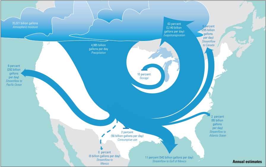
Annual average hydrologic fluxes across the conterminous United States. Precipitation data are from the bias-adjusted 4-kilometer, 40-year long-term regional hydroclimate reanalysis over the conterminous United States (Foks and others, 2024a) and evapotranspiration and streamflow data are ensembled from the National Hydrologic Model Precipitation-Runoff Modeling System (Foks and others, 2024e) and the Weather Research and Forecasting model hydrologic modeling system (Sampson and others, 2024). Consumptive use represents the sum of crop irrigation, public supply, and thermoelectric power generation consumptive use; further details are available in Medalie and others (2025; chap. D). Illustration by Althea Archer, U.S. Geological Survey.
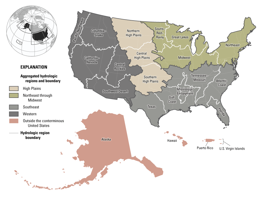
Hydrologic regions and aggregated hydrologic regions across the conterminous United States, Alaska, Hawaii, Puerto Rico, and U.S. Virgin Islands (Van Metre and others, 2020).
This chapter presents consistent, nationwide water-budget analyses at high spatial resolution with rigorously quantified uncertainty. Both models simulate water-budget components over the entire CONUS domain, whereas budget components for Alaska, Hawaii, and Puerto Rico are only simulated by NHM–PRMS. Where both models produce simulations, the average of the simulations is presented as an ensemble estimate. The spatial patterns and temporal variability, including assessment of uncertainty, provide a foundation for hydrologic understanding at the regional and national scale and for the assessment of availability under current and future conditions.
Accounting of Water-Storage Components and Fluxes
Water Fluxes—Precipitation, Evapotranspiration, and Streamflow
The principal fluxes that constitute the hydrologic cycle—precipitation, evapotranspiration, and streamflow, which comprises quickflow and base-flow components—were simulated for water years 2010–20. Precipitation was simulated by CONUS404 (Foks and others, 2024a) and evapotranspiration and streamflow components were simulated by WRF–Hydro and NHM–PRMS and ensembled (Foks and others, 2024b, 2024c, 2024d, 2024e; Sampson and others, 2024). The distributions of the results for CONUS, the aggregated hydrologic regions, and the hydrologic regions are presented in tables 1 and 2. Additionally, the spatial distribution of the annual fluxes for CONUS and OCONUS is presented in figure 3.
Table 1.
Ensemble estimates of annual cumulative precipitation and annual maximum snow water equivalent for each hydrologic region, aggregated hydrologic region, and the conterminous United States.[All values are reported in millimeters. Minimum, 25th percentile, mean, 75th percentile, maximum, and interquartile range of annual values are reported. Aggregated hydrologic regions are bolded. Abbreviations: CONUS, conterminous United States; CONUS404, the bias-adjusted 4-kilometer resolution, long-term regional hydroclimate simulation over the conterminous United States dataset (Sampson and others, 2024); Q25, 25th percentile; Q75, 75th percentile; IQR, interquartile range. Precipitation data are from the bias-adjusted 4-kilometer resolution, long-term regional hydroclimate simulation over the conterminous United States dataset (Foks and others, 2024a) and snow water equivalent data are ensembled from the National Hydrologic Model Precipitation-Runoff Modeling System (Foks and others, 2024e) and the Weather Research and Forecasting model hydrologic modeling system (Sampson and others, 2024)]
Table 2.
Ensemble estimates of evapotranspiration, quickflow, and base flow for each hydrologic region, aggregated hydrologic region, and the conterminous United States.[All values are reported in millimeters. Minimum, 25th percentile, mean, 75th percentile, maximum, and interquartile range of annual values are reported. Aggregated hydrologic regions are bolded. Abbreviations: Min, minimum; Q25, 25th percentile; Q75, 75th percentile; Max, maximum; IQR, interquartile range. Data are ensembled from the National Hydrologic Model Precipitation-Runoff Modeling System (Foks and others, 2024e) and the Weather Research and Forecasting model hydrologic modeling system (Sampson and others, 2024)]
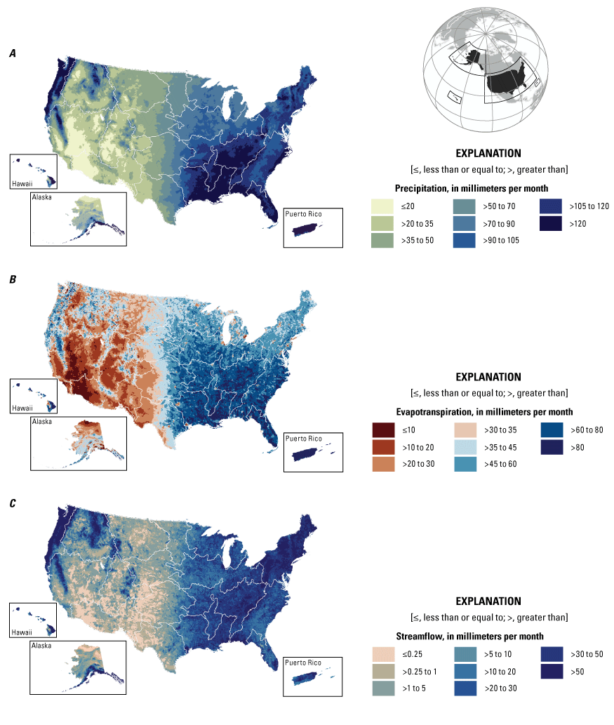
Average annual principal hydrologic fluxes in millimeters per month for (A) precipitation, (B) evapotranspiration, and (C) streamflow, in the conterminous United States, Alaska, Hawaii, and Puerto Rico. Precipitation data for the conterminous United States are from the bias-adjusted 4-kilometer, 40-year long-term regional hydroclimate reanalysis over the conterminous United States (Foks and others, 2024a). Evapotranspiration and streamflow data for the conterminous United States are ensembled from the National Hydrologic Model Precipitation-Runoff Modeling System (Foks and others, 2024e) and the Weather Research and Forecasting model hydrologic modeling system (Sampson and others, 2024). Precipitation, evapotranspiration, and streamflow data for Alaska, Hawaii, and Puerto Rico are from the National Hydrologic Model Precipitation-Runoff Modeling System (Foks and others, 2024b, 2024c, 2024d). White lines indicate boundaries between hydrologic regions.
Precipitation
Introduction
Precipitation—the process by which water vapor in the atmosphere condenses and falls to the Earth’s surface in the form of rain, snow, sleet, or hail—is a fundamental component of the hydrologic cycle and the primary input to hydrologic models and budgets. Accurate measurements and modeling of precipitation amount and timing are critical for understanding and quantifying various hydrologic processes, including surface runoff, groundwater recharge, and ET, which have direct impact on agricultural planning, water resource management, infrastructure development, and flood forecasting. In addition to precipitation, the total amount of atmospheric moisture, which represents the vertically integrated amount of water vapor in the atmosphere, is a useful indicator of the total amount of atmospheric water vapor available for precipitation at any given location.
Precipitation Results
Results from analysis of the CONUS404 dataset showed that CONUS-wide precipitation averaged 857 millimeters per year (mm/yr) of precipitation, ranging from the driest year (729 millimeters [mm] in 2012) to the wettest year (995 mm in 2019; Foks and others, 2024a). When viewed across the entire CONUS, May was the month with the most precipitation (92 mm) and January was the month with the least precipitation (58 mm).
The national scale patterns are composites of distinct regional signals that drive water availability in unique ways across the country (figs. 4 and 5). The three hydrologic regions receiving the most precipitation are the Pacific Northwest (1,688 mm annually), the Mississippi Embayment (1,470 mm annually), and Florida (1,468 mm annually). In the Pacific Northwest, cool, wet winters and warm, dry summers define precipitation patterns, with topographical effects of the Cascade Mountains strongly influencing the spatial distribution. In the Mississippi Embayment and Florida hydrologic regions, monthly precipitation totals are relatively consistent throughout the year, with high totals in the summer attributable to convective thunderstorms. Mountainous regions in the West are among the driest areas in the United States. The Central Rockies and California–Nevada hydrologic regions receive less than 450 mm/yr of precipitation, and the Columbia–Snake hydrologic region receives 643 mm/yr. These hydrologic regions are heavily dependent on winter snowfall and snowfall accumulation to sustain water resources throughout the drier summer months. This pattern is most clear in the California–Nevada and Columbia–Snake hydrologic regions, where 42 percent and 38 percent of annual precipitation falls in the winter months, respectively. The driest hydrologic region is the Southwest Desert, which receives 306 mm/yr of precipitation. This hydrologic region is heavily dependent on the Southwest monsoon, which typically delivers 37 percent of annual precipitation during the summer months. The central part of the country (including the Souris–Red–Rainy, Northern High Plains, Central High Plains, Southern High Plains, and Texas hydrologic regions) is characterized by low overall precipitation, with spring and summer periods that are wetter than the dry winters.
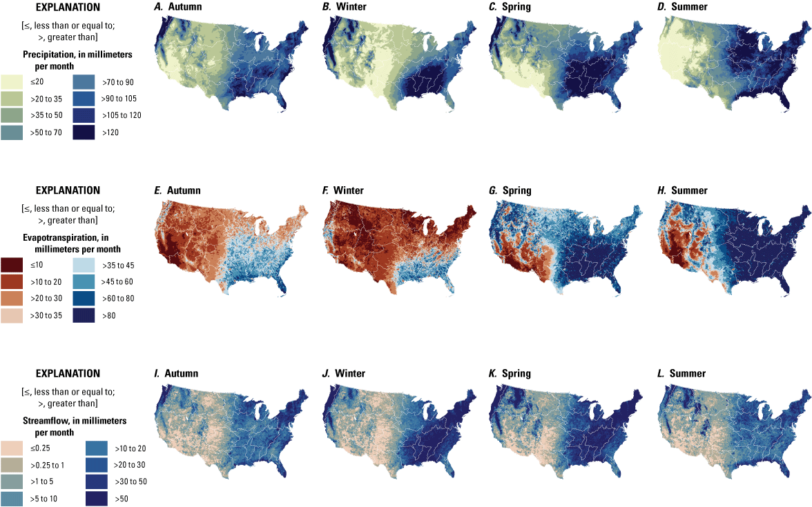
Average seasonal principal hydrologic fluxes (precipitation, evapotranspiration, and streamflow) in millimeters per month for autumn (October, November, December), winter (December, January, February), spring (March, April, May), and summer (June, July, August) from precipitation (A–D), evapotranspiration (E–H), and streamflow (I–L), across the conterminous United States. Precipitation data are from the bias-adjusted 4-kilometer, 40-year long-term regional hydroclimate reanalysis over the conterminous United States (Foks and others, 2024a) and evapotranspiration and streamflow data are ensembled from the National Hydrologic Model Precipitation-Runoff Modeling System (Foks and others, 2024e) and the Weather Research and Forecasting model hydrologic modeling system (Sampson and others, 2024). White lines indicate boundaries between hydrologic regions.
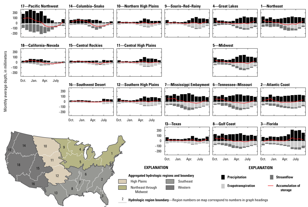
Monthly average depth for principal hydrologic fluxes of precipitation, evapotranspiration, and streamflow, by hydrologic region in the conterminous United States. Line through middle of bar graphs shows the sum of streamflow and evapotranspiration subtracted from precipitation indicating accumulation of storage. Precipitation data are from the bias-adjusted 4-kilometer, 40-year long-term regional hydroclimate reanalysis over the conterminous United States (Foks and others, 2024a) and evapotranspiration and streamflow data are ensembled from the National Hydrologic Model Precipitation-Runoff Modeling System (CONUS404; Foks and others, 2024e) and the Weather Research and Forecasting model hydrologic modeling system (Sampson and others, 2024).
The strong seasonality that defines precipitation and thus water availability in the Western aggregated hydrologic region is much less pronounced in the Northeast through Midwest and the Southeast aggregated hydrologic regions, where precipitation falls more consistently throughout the year (fig. 5). Seasonal patterns are present in the Mississippi Embayment, Tennessee–Missouri, and Northeast hydrologic regions, driven by more consistent spring and summer rains, but they are much less pronounced than those in the Western aggregated regions. The differences in seasonal patterns of precipitation drive water availability across the Nation. Many areas in the Northeast through Midwest and Southeast aggregated hydrologic regions have a more consistent water supply compared to regions in the Western aggregated hydrologic regions, which are heavily reliant on precipitation from a single season to sustain water supplies for the remainder of the year. This pattern is particularly true in snow-dominated regions (see section, “Snow Water Equivalent”).
Interannual variability in precipitation totals has a considerable effect on water availability, with more variable precipitation necessitating increased storage infrastructure, long-term planning, and diversification of water sources. Precipitation variability was assessed by calculating the coefficient of variation (CV) of the mean annual precipitation across the period of analysis, where the CV is calculated as:
whereis the population standard deviation,
is the mean,
is the precipitation in year i, and
is the number of years.
A higher CV value indicates more year-to-year variability in precipitation and lower values indicate more consistent rainfall totals. The California–Nevada and Texas hydrologic regions had the greatest CV values (0.31 in both instances), indicating that the rainfall in these regions can vary considerably from year to year. The Florida (0.08) and Tennessee–Missouri (0.11) hydrologic regions had the lowest CV values, and the average across the CONUS was 0.08.
Evapotranspiration
Introduction
Evapotranspiration (ET) is the flux of water vapor from the surface of the Earth to the atmosphere. ET encompasses two subprocesses: (1) evaporation, which occurs on the surface of waterbodies, vegetation, and bare ground; and (2) transpiration, in which plants and other vegetation transfer water from the soil and aquifer system through plant roots, stems, and eventually leaves to the atmosphere (Senay and others, 2013). ET is generally the second largest water budget component behind precipitation, and accurate estimates of ET are important for water budgeting, drought monitoring, irrigation timing, crop-yield modeling, and many other applications.
Evapotranspiration Results
According to the ensemble estimates from NHM–PRMS and WRF–Hydro, mean annual ET across the CONUS during water years 2010–20 was 539 mm/yr, about 63 percent of the average annual precipitation (Foks and others, 2024a, 2024e; Sampson and others, 2024). ET ranged from a minimum value of 488 mm in 2012 (67 percent of annual precipitation) to a maximum value of 591 mm in 2019 (59 percent of annual precipitation). Annual ET showed a strong seasonal signal with highest values of 77 mm in June and lowest values of 17 mm in December. Summertime high ET values are driven by a combination of increased transpiration from the growth of natural vegetation and agricultural crops and an increase in summer temperature and precipitation in some regions. Additionally, greater solar radiation during summer leads to greater evaporation.
In the eastern parts of the CONUS, ET is primarily limited by the available energy, resulting in a lower percentage of total precipitation recycled back to the atmosphere. By contrast, in the western parts of the CONUS, ET is often limited instead by available water. Although there are exceptions to this broad generalization, such as the Pacific Northwest hydrologic region, it explains a large amount of the regional patterns in ET across the CONUS (figs. 3B, 4E–H, 5). Model simulations show that the highest ET was in the Mississippi Embayment, Gulf Coast, and Florida hydrologic regions, where ET averaged 896, 899, and 935 mm/yr, respectively, or 61, 62, and 64 percent of annual precipitation, respectively. Areas with the lowest ET were the Southwest Desert, Alaska, and California–Nevada hydrologic regions, where ET averaged 248, 277, and 278 mm/yr, respectively or 81, 69, and 76 percent of total annual precipitation, respectively.
Seasonal patterns in ET across regions are driven by unique combinations of water supply, including soil moisture, precipitation, and surface water, and demand for ET from vegetation differing by type and coverage, solar radiation, and air temperature, and specific humidity. For example, in the Atlantic Coast hydrologic region, where precipitation is relatively constant throughout the year, ET follows a pattern similar to the CONUS-wide pattern with highs in summer and lows in winter (when most vegetation ceases transpiration after frost). In the Florida and Texas hydrologic regions, where solar radiation is consistently high, ET closely follows precipitation totals, accounting for a relatively constant fraction of precipitation (fig. 5). In contrast, areas with snowpack and summer lows in precipitation (such as the Columbia–Snake or the Pacific Northwest hydrologic regions) show highest ET earlier in the year because of melting snowpack followed by low summertime ET attributable to limited water availability even though evaporative demand is highest. In the Southwest Desert hydrologic region, late summer increases in ET are largely attributable to increased precipitation from the Southwest monsoon, a consistent, regionally important phenomena (Woodhouse and Udall, 2022).
Streamflow
Introduction
Streamflow is the flow of water in a natural channel on the land surface. Streamflow can be conceptualized as having two primary components—base flow and quickflow. Base flow is subsurface water that enters the stream channel along any reach that intersects an aquifer; it maintains streamflow between precipitation events. Quickflow is short-term drainage off the landscape following precipitation or snowmelt events. Although streamflow dynamics are often more complex, this conceptualization is useful and consistent with how fluxes are represented in the hydrologic models used in this assessment. To illustrate these definitions, in figure 6, two diagrams show stream-groundwater interactions, and an example hydrograph shows base-flow partitioning. Although streams can either gain or lose flow through connections to aquifers through bidirectional exchange (Jasechko and others, 2021), in the hydrologic models’ conceptualization of base-flow processes, base flow only adds flow to the stream.
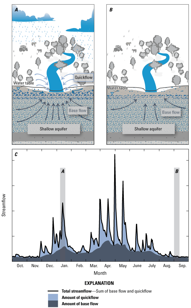
Conceptual diagrams showing (A) precipitation event with streamflow response, with total streamflow comprising quickflow and base-flow components; (B) total streamflow supplied completely by base flow from subsurface flows into stream channel, in the absence of quickflow from a precipitation event; and (C) example hydrograph with base-flow and quickflow components of total streamflow, with time periods depicted in conceptual diagrams. Diagrams show only one-way stream-groundwater interaction as conceptualized in the hydrological models, omitting bidirectional exchange processes. Illustration by Althea Archer, U.S. Geological Survey.
Streamflow Results
Analysis of ensemble results from NHM–PRMS and WRF–Hydro simulations showed that annual average streamflow across the CONUS for water years 2010–20 was 249 mm/yr (Foks and others, 2024e; Sampson and others, 2024). The lowest streamflow occurred in water year 2012 (214 mm/yr) and the highest streamflow occurred in water year 2019 (303 mm/yr). Averaged across the CONUS, the month with highest average streamflow was May (30 mm) and the month with the lowest average streamflow was August (15 mm).
Hydrographs showing total streamflow for each water year aggregated at the scale of the hydrologic region indicate distinct patterns in amount and seasonality (fig. 7). Percentile bands, calculated across the 11-year period (water years 2010–20), provide context for extreme high or low flows for the period, with the highest and lowest cumulative flow years highlighted. Consistent, distinct seasonal patterns across the period of analysis are evident in the regions most dominated by snowpack including California–Nevada, the Central Rockies, and the Columbia–Snake hydrologic regions. Seasonal patterns are also evident in the Mississippi Embayment and Tennessee–Missouri hydrologic regions; however, because the total streamflow in those regions was greater than in many regions in the Western aggregated region, a similar variability in total streamflow represents a lower percentage of flow. In the Souris–Red–Rainy, Northern High Plains, and Central High Plains hydrologic regions, streamflow was consistently lowest in winter and higher in spring and summer. In the Texas, Southern High Plains, and Southwest Desert hydrologic regions, the seasonal patterns are less obvious and emphasize the importance of event-driven streamflow there.
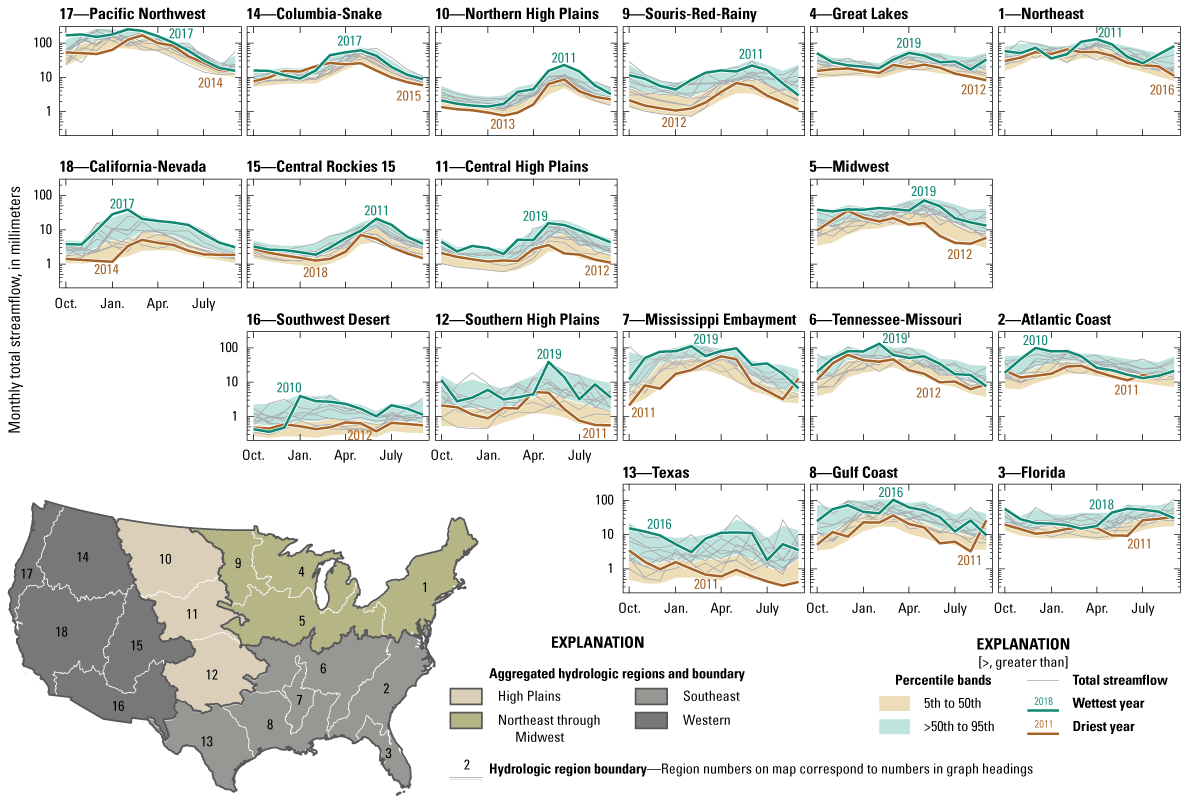
Total streamflow for each hydrologic region and map showing individual hydrologic regions and aggregated hydrologic regions, across the conterminous United States, calculated for each water year during water years 2010–20. Each annual hydrograph is shown with the year of maximum and minimum cumulative streamflow highlighted. Streamflow data are ensembled from the National Hydrologic Model Precipitation-Runoff Modeling System (Foks and others, 2024e) and the Weather Research and Forecasting model hydrologic modeling system (Sampson and others, 2024).
Annual hydrographs show that water years 2011 and 2012 had the lowest streamflow in 12 of the 18 regions, located primarily in the southern parts of the Western, High Plains, and Southeast aggregated hydrologic regions, coincident with the 2011–12 drought. This drought affected more than one-half the conterminous United States and was the most extensive drought in the United States since the 1930s, resulting in an estimated $30.0 billion ($40.5 billion in 2023 dollars) in damages and 123 attributed deaths (Smith, 2023). In the Columbia–Snake, Pacific Northwest, and California–Nevada hydrologic regions, 2017 was the water year with the highest streamflow. The elevated streamflow led to flooding in California–Nevada and was largely attributed to a deep snowpack and heavy precipitation from atmospheric river systems (Henn and others, 2020).
Total streamflow, base-flow depth, and base-flow fraction are shown for the hydrologic regions on a seasonal basis in figure 8. Base-flow depth is the area-normalized amount of base flow while base-flow fraction is the fraction of total streamflow derived from base flow and serves as an indicator of groundwater influence in the regional water supply. Within the context of the results from the models used in this assessment, which only simulate a shallow groundwater system, high base-flow fraction can indicate that inputs of subsurface water buffer a stream against short-term decreases in water supply, for example during the dry season. However, in prolonged drought, the subsurface water can become depleted making streamflow vulnerable to longer-term shifts. If shallow groundwater is also withdrawn for water use, streamflow can be substantially reduced during prolonged drought. Conversely, regions with a lower base-flow fraction have precipitation that replenishes streamflow and shallow groundwater storage on a regular basis. Highest base-flow fractions in summer, autumn and winter are simulated across the Western aggregated hydrologic regions and Northern High Plains hydrologic region where total streamflow is among the lowest of all hydrologic regions. The Pacific Northwest hydrologic region is the outlier in the Western aggregated hydrologic regions, with a distinctly lower base-flow fraction than other western hydrologic regions in all seasons except summer, emphasizing its high total streamflow and snowmelt-dominated hydrology.
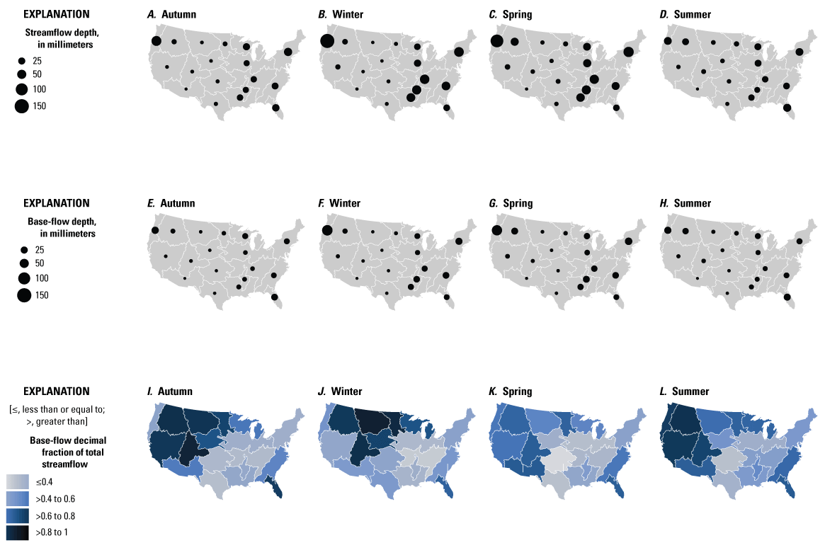
Seasonal (A–D) streamflow depth, (E–H) base-flow depth, and (I–L) base-flow fraction (base flow as a fraction of total streamflow), summarized by hydrologic region across the conterminous United States. Data are ensembled from the National Hydrologic Model Precipitation-Runoff Modeling System (Foks and others, 2024e) and the Weather Research and Forecasting model hydrologic modeling system (Sampson and others, 2024). White lines in maps indicate boundaries between hydrologic regions.
In the Western hydrologic regions during the spring, the base-flow fraction is generally lower than during other seasons, reflecting the snowmelt-dominated streamflow inputs during spring and summer in those hydrologic regions. In the eastern and central hydrologic regions of the CONUS, where total streamflow is generally higher than elsewhere in the CONUS, the base-flow fraction is lower and less variable season-to-season. The highest base-flow fraction in the Southeast aggregated hydrologic regions is present in the Florida and the Atlantic Coast hydrologic regions, which have abundant moisture year-round and where high vegetation density and ET rates may account for a higher base-flow fraction there.
Streamflow Capture and Depletion
Streamflow depletion occurs when groundwater pumping “captures” water that would have contributed to streamflow, reducing or even reversing the flow of water from a shallow aquifer to a stream (Zipper and others, 2022). Streamflow depletion may be a consequence of pumping near-stream groundwater for industrial or municipal supplies or for irrigation. It is difficult to quantify groundwater withdrawals that lead to streamflow depletion at regional scales; datasets on pumping wells are scarce and withdrawals often need to be inferred from other evidence. Several approaches using statistical or analytical methods and models have been developed recently (Zipper and others, 2022; Brookfield and others, 2024).
On a regional scale, streamflow depletion is most likely to occur where potential evapotranspiration (atmospheric demand) is greater than precipitation, although individual streams can have streamflow depletion anywhere groundwater pumping is sufficiently high. An investigation of base-flow trends and climatic drivers over a 30-year period (Ayers and others, 2022) established that precipitation deficits and rising temperatures were associated with declining base flow in the southern part of the United States whereas annual cycle shifts and increased base flow in the Northern United States were associated with increasing precipitation and temperatures. Ayers and others (2022) noted that, in addition to climate drivers, irrigation and groundwater pumping were major influences on decreasing base flow across arid and semiarid regions.
The models presented in this report treat streams and shallow, subsurface water as a linked system; streamflow at any given time comprises shallow, subsurface storage-derived base flow, with or without a quickflow component from recent precipitation or snowmelt. Future assessments can further determine the magnitude and spatial extent of net losses or gains of streamflow attributable to subsurface pumping from this linked system; for example, by addition of deep groundwater from outside the linked system through irrigation or public-supply return flows, or by capture of the base-flow volume that would occur in a setting without groundwater withdrawals. Assessment tools (for example, monitoring of changes in streams from gaining to losing, or from perennial to intermittent streams) would aid in the development of this capability. Likewise, better integration of surface water and groundwater components and, in particular, groundwater pumping for withdrawals, would also aid in the development of this capability.
Water-Storage Components—Soil Moisture, Snow Water Equivalent, and Lakes and Reservoirs
The principal water-storage components—soil moisture, storage in lakes and reservoirs, and SWE—are presented for the CONUS and OCONUS. Estimates of soil moisture were derived from NHM–PRMS (Foks and others, 2024b, 2024c, 2024d, 2024e). Static estimates of storage in lakes and reservoirs were derived from the HydroLAKES dataset (Messager and others, 2016). Estimates of SWE were derived by calculating the maximum monthly SWE for each year from the ensemble of NHM–PRMS and WRF–Hydro (Foks and others, 2024b, 2024c, 2024d, 2024e; Sampson and others, 2024). Soil moisture and SWE estimates were simulated during water years 2010–20, and annual averages were calculated to facilitate comparison across all storage components (fig. 9). The distributions of the results for the CONUS, the aggregated hydrologic regions, and the hydrologic regions are presented (table 3). Additionally, the spatial distribution of the annual storage components across the CONUS and OCONUS is presented (fig. 10).
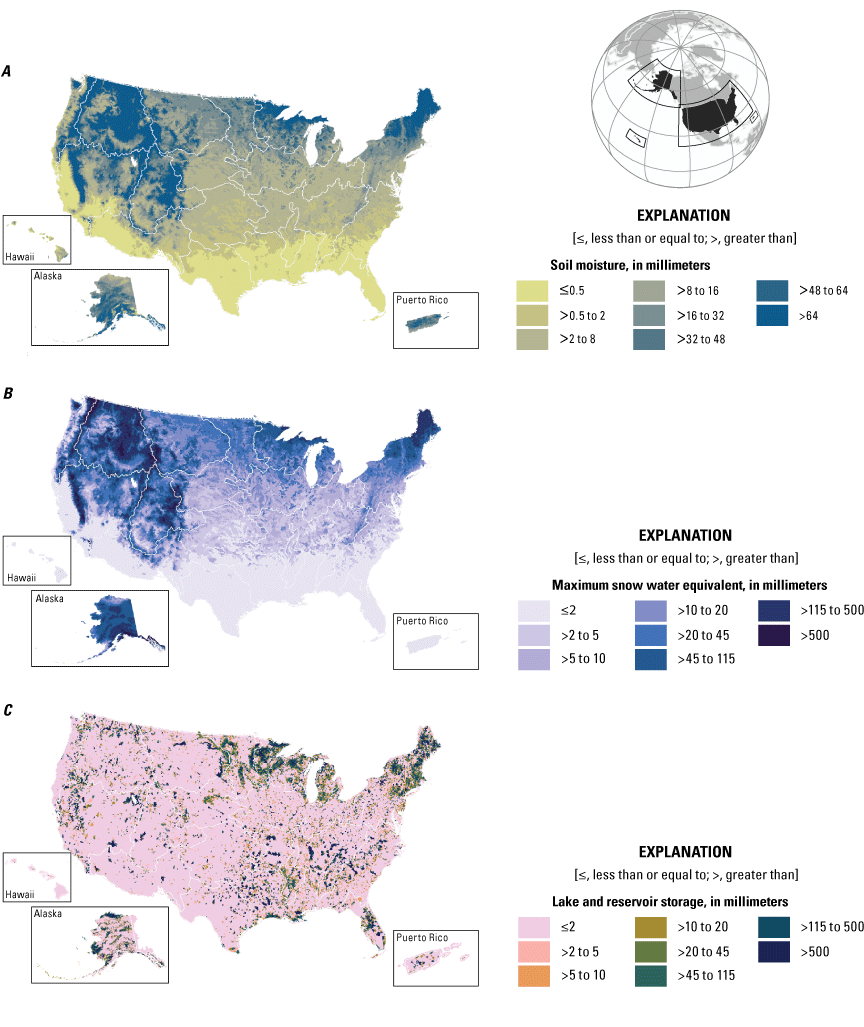
Average storage of water in (A) soil moisture, (B) maximum snow water equivalent, and (C) lakes and reservoirs in the conterminous United States, Alaska, Hawaii, and Puerto Rico. Soil moisture and snow water equivalent data for the conterminous United States are ensembled from the National Hydrologic Model Precipitation-Runoff Modeling System (Foks and others, 2024e) and the Weather Research and Forecasting model hydrologic modeling system (Sampson and others, 2024). Soil moisture and snow water equivalent data for Alaska, Hawaii, and Puerto Rico are from the National Hydrologic Model Precipitation-Runoff Modeling System (Foks and others, 2024b, 2024c, 2024d). Lakes and reservoirs data are from the HydroLAKES dataset (Messager and others, 2016). White lines indicate boundaries between hydrologic regions.
Table 3.
Average annual water-storage component for each hydrologic region in the conterminous United States, Alaska, Hawaii, and Puerto Rico.[All values are in millimeters. Abbreviations: SWE, snow water equivalent; CONUS, conterminous United States; OCONUS, outside the conterminous United States; HI, Hawaii; PR, Puerto Rico; Soil moisture and snow water equivalent data for the conterminous United States are ensembled from the National Hydrologic Model Precipitation-Runoff Modeling System (Foks and others, 2024e) and the Weather Research and Forecasting model hydrologic modeling system (Sampson and others, 2024). Soil moisture and snow water equivalent data for Alaska, Hawaii, and Puerto Rico are from the National Hydrologic Model Precipitation-Runoff Modeling System (Foks and others, 2024b, 2024c, 2024d). Lake and reservoir data are from the HydroLAKES dataset (Messager and others, 2016)]
SWE results for the OCONUS regions were simulated from the National Hydrologic Model Precipitation-Runoff Modeling System only (Foks and others, 2024a, b, c, d).
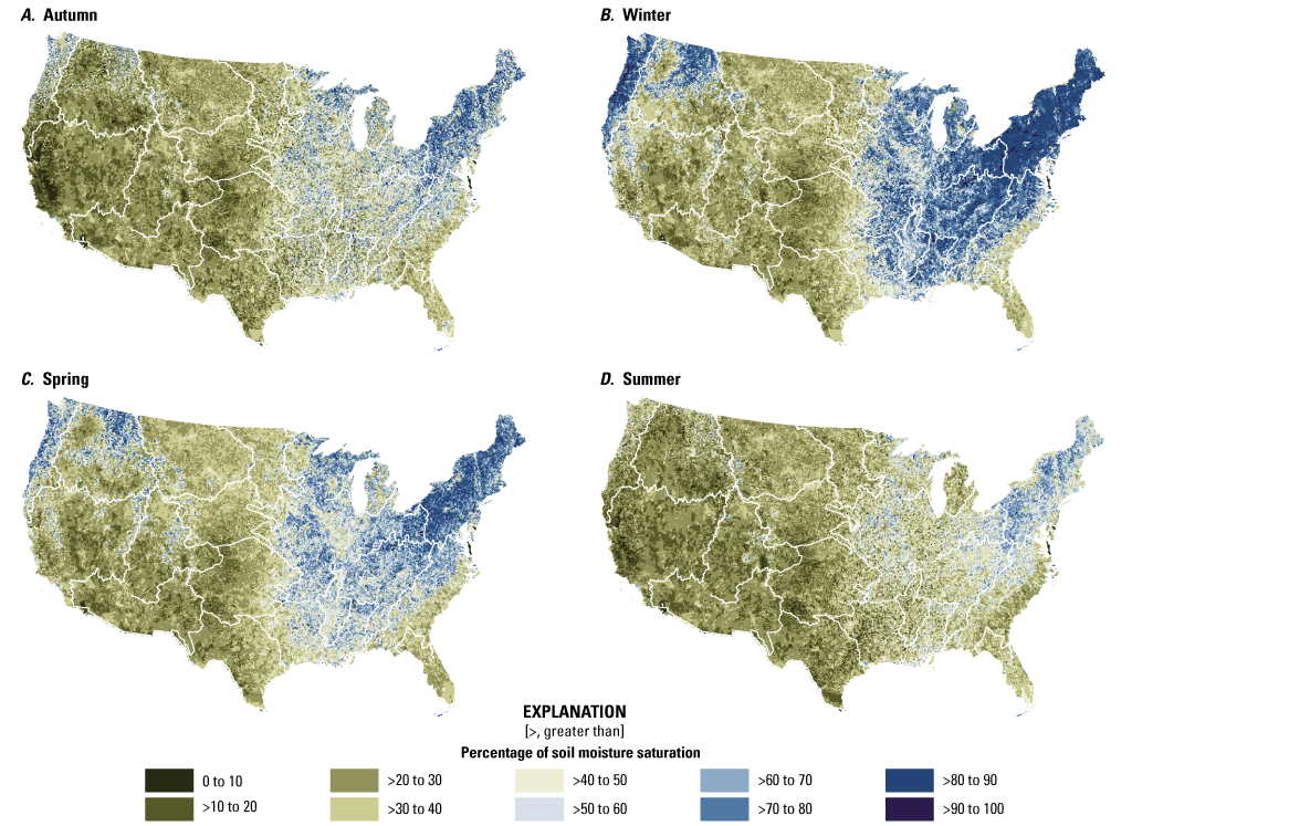
Percentage of seasonal soil-moisture saturation during (A) autumn, (B) winter, (C) spring, and (D) summer, across the conterminous United States. Data are from the National Hydrologic Model Precipitation-Runoff Modeling System (Foks and others, 2024e). White lines indicate boundaries between hydrologic regions.
Soil Moisture
Introduction
Soil moisture is a general term for water that occurs below the surface of the earth, but above the saturated zone in an area often referred to as the unsaturated zone or the vadose zone. Soil moisture plays a critical role in many hydrologic processes such as infiltration, groundwater recharge, runoff generation, and evapotranspiration (Vereecken and others, 2022). It serves as a key linkage between hydrologic, biological, and climatic processes by providing water for plants in the root zone and recycling water back to the atmosphere through plant transpiration and evaporation from bare soils (Legates and others, 2011). Soil moisture acts to partition incoming solar radiation between latent and sensible heat, which subsequently drives the climate system (Entekhabi and others, 1996; Seneviratne and others, 2010).
Although the quantity of water in the unsaturated zone can be large (Long and others, 2013), volumetric estimates of soil moisture are difficult to measure directly at applicable scales. Therefore, to compare the soil-moisture simulations from both models (WRF–Hydro and NHM–PRMS), we present relative soil-moisture volumes ranging from 0 (representing the permanent wilting point) to 1 (representing the field capacity) to emphasize the accessible part of soil water. These values are independently calculated for each model, and then averaged across the two models and multiplied by 100 to calculate percent saturation. Although the two models represent soil processes differently, this approach serves to unify the different conceptualizations of soil-water processes and facilitates the comparison of spatiotemporal patterns of available soil moisture to those seen in the benchmarking dataset.
WRF–Hydro simulates soil moisture to a depth of 2 meters (m) in a four-layer soil zone (0–10, 10–40, 40–100, and 100–200 centimeters [cm]) that can acquire a range of saturations to contribute to lateral flow, exfiltration, drainage to deeper layers, or contributions to streamflow based on an empirical storage-discharge formulation. For this report, to facilitate comparison between the models and benchmark dataset, the soil-moisture fluctuations in the top 10 cm of the soil zone were considered.
In NHM–PRMS, soil moisture is not simulated at a specific depth; rather, it is represented in two conceptual reservoirs: (1) the capillary reservoir, which represents the soil moisture between field capacity and the permanent wilting point; and (2) the gravity reservoir, in which water over the field capacity contributes to slow lateral interflow and drainage to groundwater.
In addition to soil saturation, we also present estimates of soil-moisture volumes, as simulated by NHM–PRMS, to facilitate volumetric comparisons to other fluxes and storage components. We use the combined volume in the capillary reservoir and the gravity reservoir to represent all moisture below the land surface and above the water table. To summarize soil-moisture volumes, we use the average monthly soil-moisture volume and normalize by the area to generate a depth of soil moisture.
Soil Moisture Results
Analysis of soil-moisture volumes from NHM–PRMS showed that across the CONUS, soil moisture was relatively higher in the mountainous regions of the Western United States and the northern parts of the Northeast and Great Lakes hydrologic regions, and relatively lower in the High Plains and Southeast aggregated hydrologic regions (Foks and others, 2024e; fig. 9A). Soil-moisture saturation was highest in winter, when ET was low, and lowest in summer, when demands from ET were high. Soil-moisture saturation showed similar spatial patterns to ET, with relatively higher values in the more mesic eastern part of the country and relatively lower values in the more arid West, where a relative lack of precipitation and high evaporative demand reduced soil-moisture storage, particularly in the upper layers of the soil (fig. 10).
Several hydrologic regions—such as Florida, Texas, Central Rockies, Southwest Desert, the Northern High Plains, Central High Plains, and Southern High Plains—showed minimal seasonal variation in soil moisture. In these hydrologic regions, ET and streamflow balanced precipitation and there was little accumulation of soil moisture throughout the year (fig. 5). In other hydrologic regions, seasonal highs in soil moisture occurred in winter and spring, when precipitation was high and was not matched by losses attributable to ET, as was the case in the Pacific Northwest, Northeast, Great Lakes and Mississippi Embayment hydrologic regions.
Soil moisture provides a critical storage component, which is closely tied to precipitation-streamflow dynamics in watersheds. Soil moisture can influence flood generation through rainfall-runoff response where saturation-excess mechanisms lead to flooding (Berghuijs and others, 2016; Crow and others, 2018), and knowledge of soil moisture can improve streamflow forecasts (Koster and others, 2010; Harpold and others, 2017). Soil moisture is driven by topography, vegetation, soil depth, and antecedent precipitation (Vereecken and others, 2014) and can be affected by soil properties such as bulk density and porosity at the local scale (Gaur and Mohanty, 2013). Seasonal, cumulative soil-moisture volumes were compared across hydrologic regions and time periods through normalizing by cumulative-precipitation totals, highlighting areas with strong imbalances between precipitation and storage (fig. 11). For example, soil-moisture stores in the Pacific Northwest hydrologic region in summer show the highest values (1.53 decimal fraction of 1). Summer precipitation is low in the Pacific Northwest hydrologic region, so the excess moisture helps to sustain base flow, which constitutes a large fraction of streamflow (fig. 8). In contrast, during summer in the Sours-Red-Rainy, Texas, Southern High Plains, and Southwest Desert hydrologic regions, soil-moisture volumes are low (all less than 0.07 decimal fraction of 1), indicating that the precipitation that falls during these times is directly lost to streamflow and (or) ET and relatively little is partitioned to storage. The lowest values are all present in summer, except in autumn in the Southwest Desert and Texas hydrologic regions (both 0.05 decimal fraction of 1), and in spring in the Texas hydrologic region (0.04 decimal fraction of 1). These results highlight the potential vulnerability of these hydrologic regions, as there is little storage to buffer supplies during periods of low rainfall.
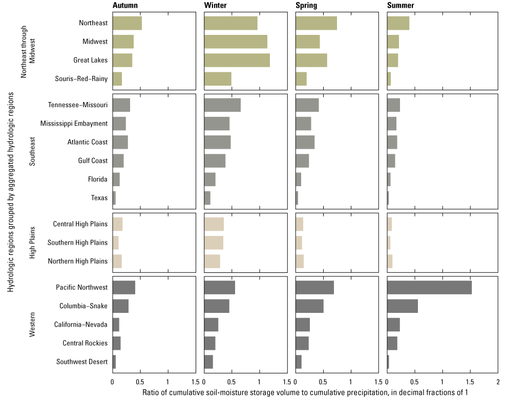
Ratio of cumulative soil-moisture storage to cumulative precipitation for each hydrologic region in each season, expressed as a decimal fraction of 1 and grouped by aggregated hydrologic regions, in the conterminous United States. Soil moisture data are from the National Hydrologic Model Precipitation-Runoff Modeling System (Foks and others, 2024e) and precipitation data are from the bias-adjusted 4-kilometer, 40-year long-term regional hydroclimate reanalysis over the conterminous United States (Foks and others, 2024a).
To assess the temporal patterns in soil moisture across the period of analysis, the minimum and maximum soil saturation for each month was calculated. The percentage of each of the aggregated hydrologic regions that had extreme soil saturation (defined as the minimum or maximum soil saturation for that month across the period of analysis) was calculated and is shown in figure 12. Extremely dry conditions were simulated in >25 percent of the Southeast aggregated region in water year 2011. In water year 2012, >75 percent of the High Plains and >60 percent of the Northeast through Midwest aggregated region had extremely dry conditions because of anomalously low rainfall totals in spring and summer. These extremely dry conditions were associated with the most severe and widespread drought in the period of analysis and one of the most extreme droughts since the 1930s dust bowl, when similar conditions were present throughout the High Plains aggregated region and much of the western part of the Northeast through Midwest aggregated region (Hoerling and others, 2014; Bell and others, 2015). Large parts of the Southeast and Northeast through Midwest aggregated regions had the wettest soil-moisture conditions in water years 2019 and 2020, whereas the Western aggregated region showed extremes in soil-moisture saturation in response to the heavy snowpack and rainfall in water year 2017.
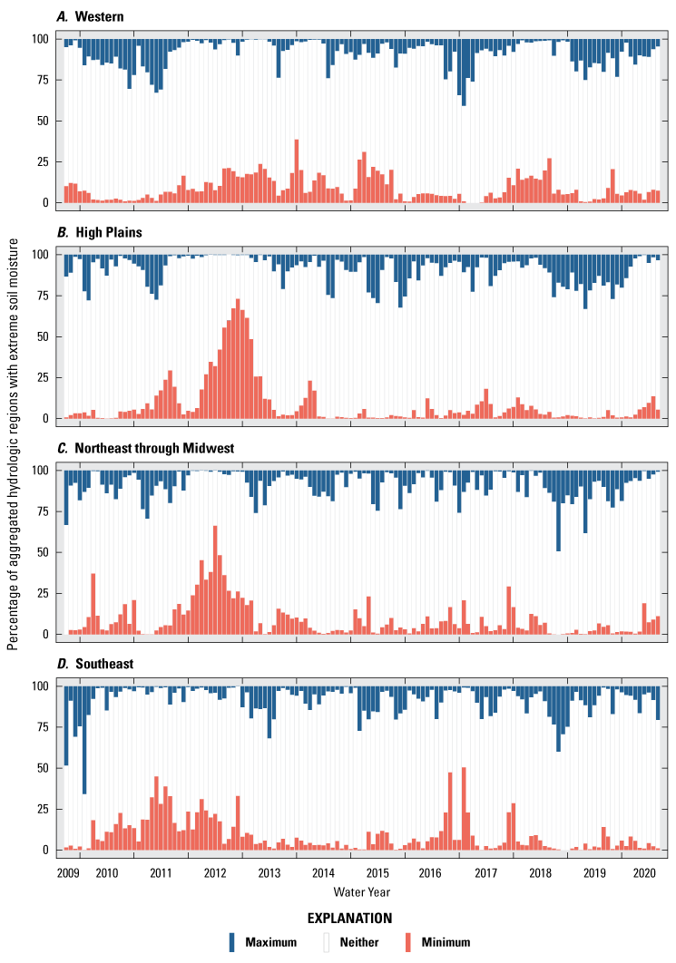
Percentage of (A) Western, (B) High Plains, (C) Northeast through Midwest, and (D) Southeast aggregated hydrologic regions with extremes in soil-moisture saturation, in the conterminous United States, calculated monthly across the period of analysis—water years 2010–20. White areas indicate neither minimum nor maximum values for a given month. Soil-moisture saturation data are ensembled from National Hydrologic Model Precipitation-Runoff Modeling System (Foks and others, 2024e) and the Weather Research and Forecasting model hydrologic modeling system (Sampson and others, 2024).
Snow Water Equivalent
Introduction
Water storage as snow is an important part of the hydrologic cycle and snowpack dynamics have a substantial influence on water availability (Dettinger, 2005). The amount of water stored as snow, which is a function of snow depth as well as snowpack density and structure, is called snow water equivalent (SWE). SWE is comparable to other hydrologic storage terms such as soil moisture and surface-water storage. SWE is a temporary storage of water that feeds soil moisture, streamflow, and downstream reservoirs, which in turn are vital to human water uses. Snowpack accumulation is limited to high-latitude and high-elevation areas, and in most places in the CONUS it melts completely during spring and summer. The cycle of snowpack accumulation and melting is important to the maintenance of base flow during summer, especially in semi-arid environments (Godsey and others, 2014).
Recent changes toward earlier snowpack melting imperil water supplies in the Western United States. Earlier melt typically occurs more slowly than later melt, allowing more of the stored water to be lost to evaporation rather than replenishing the subsurface storage that sustains dry-season streamflows and reservoir levels (Milly and Dunne, 2016; Sexstone and others, 2020). The maximum monthly amount of SWE is one measure of snow accumulation that captures the peak extent of annual accumulation without double-counting snow that persists from one month to the next, hereinafter referred to as maximum SWE. We use maximum SWE to assess spatial patterns and temporal variability in snowpack across the CONUS and OCONUS.
Snow Water Equivalent Results
Results from our analysis showed that average maximum SWE during water years 2010–20 across the CONUS was highest in the mountainous Western aggregated hydrologic regions, such as the Columbia–Snake (169 mm/yr) and Pacific Northwest (117 mm/yr) hydrologic regions (fig. 13A; table 3; Foks and others, 2024e; Sampson and others, 2024). Two hydrologic regions in the Western aggregated hydrologic region in which snowpack is an important water source showed somewhat lower maximum SWE: the Central Rockies (69 mm/yr), and the California–Nevada (48 mm/yr) hydrologic regions. The highest maximum SWE in all these hydrologic regions occurred in water year 2017. The lowest maximum accumulation in all these regions except the Central Rockies hydrologic region occurred in water year 2015; the Central Rockies hydrologic region had a lower maximum SWE in water year 2018.
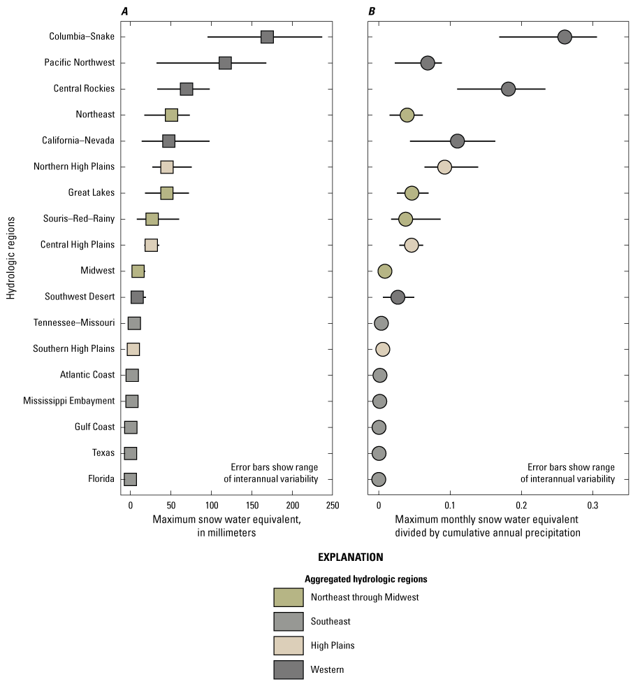
Maximum snow water equivalent (SWE) (A) and maximum SWE divided by cumulative annual precipitation (B) for each hydrologic region, grouped by aggregated hydrologic regions, in the conterminous United States during water years 2010–20. Snow water equivalent data are ensembled from National Hydrologic Model Precipitation-Runoff Modeling System (Foks and others, 2024e) and the Weather Research and Forecasting model hydrologic modeling system (Sampson and others, 2024). Precipitation data are from the bias-adjusted 4-kilometer, 40-year long-term regional hydroclimate reanalysis over the conterminous United States (Foks and others, 2024a).
Among these Western aggregated hydrologic regions, the California–Nevada hydrologic region had the highest interannual variability, with a CV of 0.60, compared to a CV of less than or equal to 0.36 for the Columbia–Snake, Pacific Northwest, and Central Rockies hydrologic regions. In the California–Nevada hydrologic region, the water year with the lowest maximum SWE (2015) showed less than 30 percent of the average maximum SWE and was among the driest on record (Margulis and others, 2016). However, just 2 years later in water year 2017, the same hydrologic region had a maximum SWE accumulation >200 percent of average. This highlights the intense year-to-year variability in western snowpacks, making interannual water storage and planning both difficult and critical (Siirila-Woodburn and others, 2021). The California–Nevada and Central Rockies hydrologic regions had regionwide average maximum SWE of 40–60 mm/yr during water years 2010–20, which was similar to other northern regions across the CONUS. More southern hydrologic regions had much lower snowpack and SWE overall.
Although SWE is an important source of water supply, especially in the mountainous Western aggregated hydrologic region of the CONUS, its accumulation is subject to extreme spatial heterogeneity, meaning that large areas of these regions rely on water supplies that originate from a limited number of HUC12s. In the mountainous hydrologic regions within the western part of the CONUS (California–Nevada, Central Rockies, Columbia–Snake, Pacific Northwest, and Southwest Desert hydrologic regions), the HUC12s with the highest snowpack accumulate several meters of SWE during the cold months, which is much larger than the regionwide average. The Central High Plains and Northern High Plains hydrologic regions also contained HUC12s that could accumulate >1 m of maximum SWE. In other parts of the northern CONUS, the snowiest HUC12s accumulate several hundred millimeters of SWE.
The relative importance of SWE to water supply can be expressed as its ratio to annual precipitation (SWE/P). Maximum SWE in a HUC12 is the total amount of water stored as snowpack that can potentially become available for water supplies during snowmelt. This amount, in comparison to annual precipitation, provides perspective on the potential importance of SWE to overall water supplies. The Columbia–Snake, Central Rockies, and California–Nevada hydrologic regions had the highest average SWE/P; all were >0.1 (fig. 13B). Other hydrologic regions in the northern CONUS had much lower SWE/P despite having appreciable maximum SWE. The Souris–Red–Rainy, Great Lakes, Northeast, and Central High Plains hydrologic regions all had SWE/P values less than 0.05 (fig. 13B). Other parts of the CONUS had still lower values. However, SWE/P also had high spatial heterogeneity, as was also the case with maximum SWE.
Snow persistence (SP) is the amount of time that snow remains on the ground over a given time period, which can be useful for determining the geographic extent of snow coverage regimes; the timing of melt generation; and the boundaries between zones of low, intermittent, and persistent snow coverage (Bales and others, 2006). Following previous work, we defined ranges of SP for January–July of each year to compare coverage across hydrologic regions (Hammond and others, 2018; fig. 14). Any HUC12 was considered to have snow for a given month if SWE was >10 mm, and each HUC was classified as having (1) low snow if SP was less than or equal to (≤) 3 months; (2) intermittent snow if SP was >3 months and ≤6 months; or (3) persistent snow if SP >6 months. This analysis revealed that, in the snowiest hydrologic region of the CONUS (the Columbia–Snake hydrologic region), 53 percent of the region had at least intermittent snow, indicating relatively widespread snow coverage during the winter, whereas only 6 percent of the hydrologic region had persistent snow (fig. 14D). In contrast, in the Central Rockies and California–Nevada hydrologic regions—two regions that are heavily dependent on snowmelt for water availability—only 27 and 14 percent of the hydrologic regions had at least intermittent snow, respectively, and 4 percent and less than 1 percent had persistent snow, respectively (fig. 14D). The mountains of the Western United States are commonly referred to as the “water towers” of those areas because of their importance to water supply, especially during snowmelt in summer and early autumn (Viviroli and others, 2007; Scholl and others, 2025). The snow persistence results of the Western aggregated hydrologic regions (fig. 14A) align with the “water tower” perspective and emphasize that SWE storage and persistence have a skewed spatial distribution such that a small proportion of these regions is responsible for a large amount of the SWE storage and subsequent water supply in the regions.
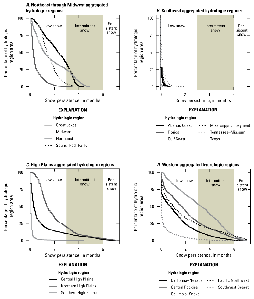
Snow persistence (SP) as number of months from January through July in which each 12-digit hydrologic unit code had a snow water equivalent greater than 10 millimeters, across the conterminous United States, averaged for water years 2010–20. To view snow persistence, we plotted the cumulative percentage of area in each hydrologic region with less than a certain amount of SP within the (A) Northeast through Midwest, (B) Southeast, (C) High Plains, and (D) Western aggregated hydrologic regions. Low snow indicates SP less than or equal to (≤) 3 months, intermittent snow indicates SP was greater than (>) 3 months and ≤ 6 months, and (3) persistent snow indicates SP was > 6 months. Snow water equivalent data are ensembled from the National Hydrologic Model Precipitation-Runoff Modeling System (Foks and others, 2024e) and the Weather Research and Forecasting model hydrologic modeling system (Sampson and others, 2024).
Lakes and Reservoirs
Introduction
The storage of fresh water in lakes and reservoirs is a critical component of the hydrologic cycle, providing for water supply, as well as biogeochemical and ecological processing functions (Cole and others, 2007). Lakes and reservoirs are crucially important for water storage and can buffer water supplies during periods of low precipitation. The construction of reservoirs for water supply, flood control, recreation, hydropower, or other purposes has helped facilitate rapid growth and population expansion, particularly in the Western United States, but has also had a large impact on hydrologic flows (Magilligan and Nislow, 2005; Harvey and Schmadel, 2021). Although many of the largest lakes and reservoirs have well-characterized size, capacity, and fluctuations in storage volume, many of the smaller waterbodies, although still important, are less well-characterized. Neither of the hydrologic models used in this assessment simulate the amount of storage in lakes and reservoirs, so external sources were used to assess this storage component.
To estimate the water storage in lakes and reservoirs, we used the HydroLAKES global spatial dataset (Messager and others, 2016), the result of a geostatistical model using land-surface topography, which estimates the volume, surface area, and residence time of lakes with a surface area of 0.10 km2 and greater. This dataset provides a fixed estimate of lake characteristics, and therefore, represents a static upper limit of storage capacity. The time-varying component to water storage in lakes and reservoirs is a first-order consideration, attributable to the drawdown of lake and reservoir volumes that occurs as a result of drought and (or) increased use. Such temporal dynamics are not captured in our assessment; nevertheless, the static estimate can provide important information examining regional differences and overall hydrologic budgets. The accuracy of the HydroLAKES dataset was estimated by comparing the modeled lake volume to independent datasets, which revealed a global coefficient of determination (R2) =0.92, with higher uncertainty associated with smaller lakes. The HydroLAKES dataset includes natural lakes and human-made reservoirs by incorporating data from the Global Reservoir and Dam database (Lehner and others, 2011). The HydroLAKES dataset includes coverage of the CONUS, OCONUS, and U.S. Virgin Islands. Lake- and reservoir-storage volumes are presented for all of these areas, but comparison to other storage components does not include the U.S. Virgin Islands and is limited to the CONUS and OCONUS.
Lake and Reservoir Results
Our analysis of the HydroLAKES dataset shows that the CONUS, OCONUS, and U.S. Virgin Islands have a total of 102,528 natural lakes and 1,891 reservoirs, with volumes of 23,567 and 715 km3, respectively (Messager and others, 2016). This is equivalent to 2,416 and 73 mm, respectively, when converted to a depth by dividing by the combined area of the CONUS, OCONUS, and the U.S. Virgin Islands, or a total of 2,489 mm. The Great Lakes (Lakes Superior, Michigan, Huron, Ontario, and Erie) store >95 percent (22,553 km3) of the total volume of lakes in the CONUS, OCONUS, and U.S. Virgin Islands. For this reason, the Great Lakes are broken out separately for the regional analysis, and their storage volumes are not attributed to any hydrologic region (fig. 15A, note the different scale). These large lakes and reservoirs, including the Great Lakes, contribute considerable storage during dry seasons and dry years, and are of substantial regional and national importance to water supply. Additionally, complex networks of water transfers have been developed that allow for water to be moved across hydrologic boundaries to buffer water supplies in other basins and regions (Siddik and others, 2023). Aside from the Great Lakes, the volume of water stored in reservoirs constitutes about 41 percent of total storage in lakes and reservoirs across the CONUS, OCONUS, and U.S. Virgin Islands. Although there are relatively few reservoirs compared to natural lakes, they are of great importance from a water-supply perspective. The spatial distribution of lakes and reservoirs is reflective of several natural and anthropogenic factors including natural depressions and more humid conditions in the Northeast through Midwest aggregated hydrologic regions, with recent glaciation and large constructed reservoirs in the Western aggregated regions (Brosius and others, 2021). When each of the Great Lakes is assessed individually and all other lakes and reservoirs are grouped by hydrologic regions, volume and surface area are highly correlated, with some exceptions (including the Great Lakes hydrologic region), indicating potentially shallower average lakes and reservoirs than in the rest of the hydrologic regions (fig. 15B). The California–Nevada hydrologic region stands out, with a large volume relative to surface area and number of lakes and reservoirs, largely because of the considerable volume of water stored in Lake Tahoe, which accounts for about 46 percent of the total lake and reservoir storage in that region. Hydrologic regions with lower total volume of storage generally show a higher fraction of that storage in reservoirs compared to lakes (fig. 15C). For example, Alaska is the hydrologic region with the highest volume and surface area and with approximately 100 percent in lakes, whereas The Mississippi Embayment hydrologic region has the lowest water storage in the CONUS and with >95 percent in reservoirs. Mountainous hydrologic regions (such as the Central Rockies, Columbia–Snake, and California–Nevada hydrologic regions) have more lake storage than reservoirs, whereas >90 percent of storage volume in the hydrologic regions of Texas, Southern High Plains, Tennessee–Missouri, and Central High Plains is within reservoirs.
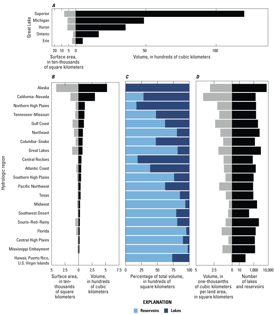
(A) Distribution of lake and reservoir combined surface area and (B) volume for the Great Lakes and hydrologic regions; (C) percentage of total volume within each region that is stored in lakes and reservoirs, respectively; (D) and lake and reservoir density in volume per land area and the number of lakes and reservoirs within each hydrologic region, in the conterminous United States, Alaska, Hawaii, Puerto Rico, and the U.S. Virgin Islands. The five Great Lakes are plotted separately in (A) with a different scale, and the values plotted in graphs (B) and (C) labeled “Great Lakes” refer to the hydrologic region, not the lakes themselves. Data from the HydroLAKES dataset (Messager and others, 2016).
The density of lakes and reservoir storage was calculated by dividing the total volume by the land surface area of the hydrologic region (fig. 15D). This showed that the Alaska, California–Nevada, the Gulf Coast, and the Northern High Plains hydrologic regions had the highest storage density. The Alaska hydrologic region has 59,481 lakes, more than six times more than the next highest hydrologic region, the Great Lakes hydrologic region (with 9,574 lakes). The Southwest Desert hydrologic region and the combined area of Hawaii, Puerto Rico, and the U.S. Virgin Islands constitute the other end of the distribution, with 222 and 70 total lakes and reservoirs, respectively.
Like the distribution of lakes worldwide, the number of lakes in the United States is skewed towards small lakes (that is, volume less than or equal to 0.1 km3; fig. 16). These small lakes are important for aquatic terrestrial interface (Pi and others, 2022) yet contribute less to storage of water. For example, our analysis showed that all but 1,212 lakes and reservoirs have a volume of ≤0.1 km3, accounting for 99 percent of the total number of lakes and reservoirs; however, these waterbodies account for only 1 percent of the total volume stored in lakes and reservoirs throughout the CONUS, OCONUS, and the U.S. Virgin Islands. Although the exact distribution of surface areas and volumes is uncertain, especially with regard to the abundance of small lakes, the analysis using modeled volumes referenced here addresses the regional trends and volume of water in lakes and reservoirs nationwide, and likely still holds true despite this uncertainty (McDonald and others, 2012; Verpoorter and others, 2014).
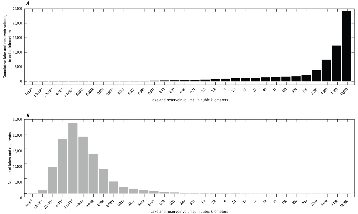
Cumulative lake and reservoir volume (A) and number of lakes and reservoirs binned by lake volume (B) across the conterminous United States plus Alaska, Hawaii, Puerto Rico, and the U.S. Virgin Islands. Figure shows that most lakes are relatively small but that the cumulative lake and reservoir volume is controlled by a small number of large lakes. Data from the HydroLAKES dataset (Messager and others, 2016).
Groundwater Resources
Introduction
Groundwater is an important component of water supply for domestic use and in various economic sectors, including agriculture, livestock, mining, and industrial applications, and most of groundwater use is derived from fresh groundwater reserves (Dieter and others, 2018). In water year 2020, about 65,406 million gallons per day (Mgal/d) extracted from aquifers accounted for 65 percent of all irrigation applications, the highest percentage for any single use (chap. D, Medalie and others, 2025). Additionally, in water year 2020, groundwater withdrawn from public supply wells totaled 13,725 Mgal/d, accounting for 51 percent of the public supply across the CONUS. Most withdrawals come from relatively few regionally important aquifers (fig. 17). Reilly and others (2008) estimated that only 30 principal aquifers in the CONUS and OCONUS were responsible for supplying about 94 percent of the Nation’s total groundwater withdrawals.
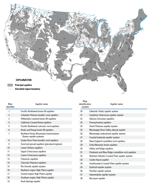
Selected principal and regional aquifers in the conterminous United States included in this analysis. Aquifer boundaries were derived from the U.S. Geological Survey (2003), and Upper Midwest Water Science Center (2002).
Groundwater also plays a critical role in maintaining the health of ecosystems through discharges to estuaries, stream channels, and surface waterbodies (Rosa and others, 2023). Groundwater contributes to minimum in-stream flows (base flow) and modulates surface-water temperatures and the water quality. Dependence of ecosystems on groundwater has been widely recognized (Jakeman and others, 2016) and groundwater plays a critical role in maintaining the health of aquatic habitats (Saunders and others, 2001; Essaid and Caldwell, 2017). Regional assessments and models have shown that pumping of deep, regional groundwater resources can affect shallow groundwater supplies and associated contributions to base flow, as is discussed further in the “ Streamflow” section of this chapter and in chapter E of this professional paper concerning future water availability (chap. E, Scholl and others, 2025).
The national budgets of stores and fluxes presented in the previous sections of this chapter have focused on results from national models primarily focused on surface water, soil moisture-vegetation processes, and shallow upper parts of aquifers. Although groundwater plays a critical role in water supply, assessments of groundwater availability and its variation in space (depth and distance from recharge) and time, including flow rate and age, are subject to challenges that are not encountered in the evaluation of surface-water resources. Groundwater flow is largely unobserved, apart from where it naturally discharges at the land surface from springs and to streambeds as base flow, at engineered abstraction points (such as pumping wells), in monitoring wells, and indirectly with geophysics and remote sensing.
Regional aquifers used as water supplies include (1) principal aquifers (U.S. Geological Survey, 2000); (2) secondary hydrogeologic regions (Belitz and others, 2019); and (3) areas of permeable overlying glacial sediment, coarse glacial sediment, and stream valley alluvium (alluvium). Glacial deposit maps were developed to assess regional aquifer productivity (Yager and others, 2019). Alluvium was mapped in areas south of the maximum extent of glaciation that were defined either as alluvial sediments or coarse-grained proglacial sediments (Soller and others, 2009). The extent of aquifers does not align with the hydrologic regions delineating surface-water budgets, further complicating contributions of groundwater to water budgets.
In this section, we summarize past and present groundwater-level data from representative wells in principal and regional aquifers throughout the CONUS to identify areas where water levels are increasing, stable, or decreasing. Although groundwater levels are not the only component of groundwater availability, they represent an important proxy for current conditions that has widespread spatial coverage.
Previous Assessments
National assessments of groundwater availability have immense value and have generally been conducted in two ways:
-
1. Using regional hydrologic investigations and regional groundwater-flow modeling (Reilly and others, 2008); and
-
2. More recently, with remote sensing using Gravity Recovery and Climate Experiment (GRACE) satellite observations in conjunction with groundwater modeling and observations of groundwater storage (for example, Rateb and others, 2020).
Regional or CONUS-wide assessments of the water-budget components associated with shallow groundwater are also outcomes from surface process models used in this assessment (Regan and others, 2018; Gochis and others, 2020). These investigations have estimated components of recharge to groundwater or aquifer discharges, but they do not necessarily identify the recharge or discharge associated with principal aquifers and examine the significance of those aquifer fluxes in relation to water uses. Water-budget components in the principal aquifers are best assessed through groundwater-flow models and data interpretations that specifically analyze hydraulic responses over the geologic extent of a principal aquifer of interest. Recharge, discharge, and changes in storage for an aquifer in relation to groundwater uses can be determined from model results documented in U.S. Geological Survey (USGS) regional aquifer system analysis reports and shown in some examples from recent USGS studies (for example, Campbell and Coes, 2010; Ely and others, 2014; Alley and others, 2018).
Models of groundwater flow processes (Harbaugh, 2005; Langevin and others, 2017) and models of surface process that route water on the land surface from precipitation, snowmelt, and irrigation (Westenbroek and others, 2010; Regan and others, 2018; Gochis and others, 2020) have also been used nationally and regionally to infer estimates of the groundwater volume and rates of groundwater recharge and discharge. Groundwater-flow and surface-process models are developed from mass-balance concepts where the sources and sinks of water to these models are the spatially and time-varying meteorological conditions and anthropogenic stresses (for example, groundwater injections and abstractions, applied irrigation, surface-water diversions, etc.).
Recharge
The estimation of groundwater recharge from low-flow or base-flow metrics has been used on an annual water budget basis in humid, semi-arid, and arid environments (Lerner, 1998; Scanlon and others, 2002; Healy, 2010; Singh and others, 2018). Other physical-flow and chemical-tracer methods of estimating groundwater recharge in unsaturated and saturated systems have been developed for various spatial and temporal scales (Lerner, 1998; Cook and Bohlke, 2000; Scanlon and others, 2002; Healy, 2010).
Recharge to the subsurface at regional scales is most commonly computed using a water-balance approach as the available liquid precipitation and snowmelt after the effects of surface runoff and evapotranspiration have been subtracted (Reitz and others, 2017). However, focused recharge may also occur under natural surface-water drainages, where the groundwater table lies below the bottom of the streambed, wetland, or lake (Healy, 2010; Jasechko and others, 2021). Recharge can also occur in response to (1) engineered applications of water (such as irrigation of agricultural lands), (2) losses through the associated irrigation infrastructure (such as distribution canals), and (3) losses from hydropower and transportation canals. Recently, a workflow was established to produce yearly CONUS-wide estimates of groundwater recharge at 800-m resolution using a data-driven approach that calculates recharge as the residual from subtracting quickflow runoff and ET from irrigation and precipitation (Reitz and others, 2017).
Groundwater Storage
Quantifying the groundwater available for use is more complex than conducting a volumetric accounting of water below the land surface. The availability of groundwater also depends on socio-economic and environmental constraints (Alley, 2007). Supplying groundwater to communities may not be economically viable in low-permeability geologic materials, whereas water demands for individual dwellings can be practically and economically designed in such settings. Similarly, there are economic constraints on the depth at which groundwater can be withdrawn for public-supply and private-domestic wells. Because groundwater and surface water are an integrated resource, withdrawals of groundwater also can affect the water available in surface-water features, which may be critical for downstream domestic use and the health of ecosystems. Consequently, without establishing the existing constraints on groundwater withdrawals, it is typically more relevant to quantify groundwater availability in the context of changes in groundwater storage from a prior state or baseline condition. In this analysis, the annual median water levels were determined for water years 2000–20, and water levels for the period of analysis (water years 2010–20) were compared to the entire period to assess recent changes in water level. The scope of the analysis is necessarily limited by the number of wells in each aquifer and water-level record length at each site.
Methods
Changes in the depth of groundwater at representative monitoring locations provide an easily identifiable metric from which to visualize changes in groundwater storage. The USGS developed summaries of the status of groundwater levels and trends over the prior 21-year period (water years 2000–20) in 38 of the 67 principal and regional aquifers across the CONUS. The 38 aquifers analyzed accounted for about 82 percent of the aquifer withdrawals in the CONUS, OCONUS, and U.S. Virgin Islands in calendar year 2015 (Lovelace and others, 2020). The High Plains aquifer was divided into three regions for this analysis (north, central, and south) as done in previous efforts to estimate water-budget components in the High Plains aquifer (Stanton and others, 2011). Wells from aquifer systems with confined and unconfined aquifers were separated by confinement status and analyzed separately. Some aquifer systems have confined and unconfined parts such as the northern region of the High Plains aquifer, or the Basin and Range basins-fill aquifers. In these cases, the aquifers were analyzed separately for confined and unconfined conditions. We analyzed data from a total of 29 unconfined and 23 confined aquifers. Compared to confined aquifers, unconfined aquifers generally are nearer to the land surface and have the water table as the upper extent of the saturated zone. Confined aquifers are typically deeper than unconfined aquifers and are bounded by confining layers (aquitards) above and below (Freeze and Cherry, 1979).
Water-level data for each aquifer were downloaded from the National Groundwater Monitoring Network (NGWMN; U.S. Geological Survey, 2023a) using the dataRetrieval package in R (DeCicco and others, 2023). Data providers to the NGWMN provide the information on whether a well is monitoring a confined or unconfined aquifer. Data were retrieved from the NGWMN in April 2023, resulting in about 281,000 individual water-level measurements at 6,750 wells that had data in water years 2000–20. Water-level measurements were collected at varying temporal frequencies across the sites, and for those sites with multiple measurements in a single day, a daily measurement was randomly selected. In order to analyze data for an entire aquifer, the annual median water levels were determined for each well, and subsequently the annual water level of the aquifer was determined from a median of all wells in the aquifer. To be included in the analysis, each well had to have at least one water-level measurement during each water year 2000–20. This approach has been used for developing datasets to create aquifer composite hydrographs as described in Myers (2022).
An annual median water level was computed for each principal and regional aquifer and aquifer type (confined or unconfined) with at least 10 wells, and the annual aquifer-wide groundwater-level percentiles for these water levels were determined for water years 2000–20. Other aquifers with data in the NGWMN had an insufficient number of wells with long-term data for analysis. The medians of the calculated percentiles for the 11-year period (water years 2010–20) are presented in figure 18 and tables 4 and 5.
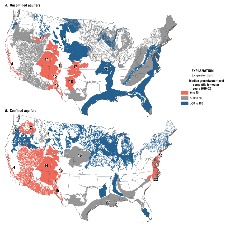
Median groundwater-level percentiles, by principal and regional aquifer, for (A) unconfined aquifers and (B) confined aquifers, in the conterminous United States across the period of analysis (water years 2010–20). Aquifer boundaries were derived from U.S. Geological Survey (2003) and Upper Midwest Water Science Center (2002). Groundwater-level data are from the National Groundwater Monitoring Network (U.S. Geological Survey, 2023a). See table in figure 17 for the names of the aquifers to which the map identification numbers in figure 18 refer. Principal aquifers without sufficient data in the National Groundwater Monitoring Network at the time of analysis are not depicted on the map. In all, 29 unconfined and 23 confined principal aquifers were included in the analysis.
Table 4.
Groundwater-level percentiles and number of wells used for analysis for unconfined principal and regional aquifers, in the conterminous United States, water years 2010–20.[Aquifer boundaries were derived from U.S. Geological Survey (2003) and Upper Midwest Water Science Center (2002). Groundwater-level data are from the National Groundwater Monitoring Network (U.S. Geological Survey, 2023a)]
Table 5.
Groundwater-level percentiles and number of wells used for analysis for confined principal and regional aquifers, in the conterminous United States, water years 2010–20.[Aquifer boundaries were derived from U.S. Geological Survey (2003) and Upper Midwest Water Science Center (2002). Groundwater-level data are from the National Groundwater Monitoring Network (U.S. Geological Survey, 2023a)]
Groundwater Resources Results
Analysis of groundwater-level data from wells in unconfined aquifers showed that six aquifer systems had median groundwater-level percentiles less than (<) 30: (1) California Coastal Basin aquifers, (2) Colorado Plateaus aquifers, (3) central and (4) southern regions of the High Plains aquifer, (5) Rio Grande aquifer system, and (6) Snake River Plain basaltic-rock aquifers, indicating that the water levels were considerably lower than normal during water years 2010–20, relative to the 21-year period analyzed (fig. 18A; table 4; U.S. Geological Survey, 2023a). A threshold of the 30th percentile was chosen to highlight those aquifers with the lowest median groundwater levels. Several other aquifer systems had median groundwater-level values less than the 50th percentile, including the Basin and Range and Pacific Northwest basin-fill aquifers, as well as the Edwards-Trinity aquifer system and Pennsylvanian and Rush Springs aquifers. The median water-level percentiles in 14 of the unconfined aquifers, or about one-half of them, were >50, but only 2 aquifer groupings were >70 (the lower Tertiary aquifers and the Ozark Plateaus aquifer system; fig. 18A; table 4).
Our analysis of groundwater-level data from wells in confined aquifers showed results similar to those of the analysis for unconfined aquifers. Six aquifers had median groundwater-level percentiles <30 percent: (1) Basin and Range basin-fill aquifers, (2) California Coastal Basin aquifers, (3) Colorado Plateaus aquifers, (4) Colombia Plateau basaltic-rock aquifers, (5) Northern Atlantic Coastal Plain aquifer system, and (6) Rio Grande aquifer system (fig. 18B; table 5; U.S. Geological Survey, 2023a). Several other aquifers had median groundwater-levels <50 percent, including the Castle Hayne aquifer, northern region of the High Plains aquifer, Northern Rocky Mountains Intermontane Basins aquifer systems, Willamette Lowland basin-fill aquifers, and Coastal lowlands aquifer system. No confined aquifers had median water-level percentiles >70 percent (fig. 18B; table 5).
The analysis of groundwater-level data has some important limitations. Data availability is not evenly distributed among aquifers and subjectivity surrounds decisions about what constitutes a representative and sufficient record for inclusion in this analysis. The limited data availability resulted in some aquifers having a minimal number of wells (tables 4 and 5). Some of the aquifers analyzed had as few as 10 wells, which may not be representative of the entire aquifer. Additionally, the 21-year period of analysis was selected to include as many sites and aquifers as possible in the analysis. Many of these aquifers have documented depletion of groundwater that began during the 20th century (Konikow, 2013), so the starting point (water year 2000) was a time when some aquifers were already depleted, resulting in water levels that had already begun to decline well before the start of our analysis.
One of the major aquifers absent from this analysis is the Central Valley aquifer system in California, which is estimated to account for about 14 percent of the annual freshwater use in the CONUS, OCONUS, and the U.S. Virgin Islands, or >11,000 Mgal/d in 2015 (Lovelace and others, 2020). Other aquifers with considerable water use, missing from this analysis, include the Columbia Plateau basin-fill aquifers (391 Mgal/d) and the Texas coastal uplands aquifer system (375 Mgal/d; Lovelace and others, 2020). These aquifers were not included in the analysis because of insufficient data in the NGWMN.
Aquifers with low groundwater levels during water years 2010–20 likely represent a general decline in water levels in this 11-year period relative to the 21-year period; for example, the confined and unconfined Colorado Plateaus aquifers where the maximum percentile was 50 for both aquifer types and median percentiles were less than 30 (tables 4 and 5). However, some aquifers showed a wider range of variability throughout the period of analysis; for example, the confined Southeastern Coastal Plain aquifer system had a median groundwater-level percentile of 50 and minimum and maximum percentiles of 4.5 and 90.9, respectively, indicating water-level response to shorter-term events (table 5).
The central and southern regions of the High Plains unconfined aquifer system offer examples of clear declines over the period of analysis relative to water years 2000–20. These declines are part of the history of groundwater-level declines that have dated back to the middle of the 20th century, when irrigated agriculture became widespread in the area (McGuire, 2013). The High Plains aquifer supplies 12,300 Mgal/d, of which nearly 95 percent is used for irrigation (Lovelace and others, 2020). Although irrigation withdrawals are high in the northern region of the High Plains aquifer, water levels have not shown the same degree of consistent decline, owing largely to the differences in natural recharge, which is higher in the northern region and lower in the central and southern region of that aquifer (Scanlon and others, 2012). This pattern has led to the conclusion that much of the withdrawals in the central and southern region are from “fossil groundwater” that was recharged over the last 13,000 years (McMahon and others, 2004). The declines in water level in this analysis have occurred even as withdrawals from the High Plains aquifer decreased by 32 percent (in 2015 relative to 2000; Lovelace and others, 2020), suggesting that despite efforts to reduce levels of groundwater withdrawal, these withdrawals are far from balanced with natural recharge.
The analysis of the status of groundwater storage for this study aligns with previous analyses of groundwater storage for principal aquifers (Konikow, 2013). Aquifers with groundwater-level percentiles <50 in this analysis that were also identified as depleted in the Konikow analyses include the High Plains aquifer, Coastal lowlands aquifer system, and North Atlantic Coastal Plain aquifer system. The depletion could be a result of a combination of factors including increases in use and (or) decreases in natural recharge from shifts in climate or land use. The results from this analysis differ from previous results for the Cambrian-Ordovician and Mississippi embayment aquifer systems, where groundwater levels during water years 2010–20 were in the normal range (>30th percentile) relative to the 21-year period. Differences can likely be attributed to different methods and time periods of analysis. Additionally, some of the aquifers were split into smaller local aquifers in previous studies, making direct comparisons difficult.
Alternative Water Resources
Alternative water resources are sources of water, not supplied from surface water or groundwater, that offset the demand for freshwater resources. Rainwater harvesting and wastewater reuse are two techniques for using alternative water resources that seek to increase water supplies that are generally for non-potable uses such as toilet flushing, laundry, dust suppression, and landscape irrigation to relieve pressure on drinking-water resources. Rainwater harvesting is generally implemented in urban areas using rooftop collection and storage systems that collect water during precipitation events (Campisano and others, 2017). Water reuse reclaims water from various sources such as municipal wastewater, industry processes and cooling water, stormwater, and produced water from natural-resource extraction for further use (Drewes, 2005). These waters generally have to be treated to meet water-quality requirements for use and can also be treated for drinking-water purposes (Lahnsteiner and others, 2017).
Desalination is a technique that has grown in popularity partly owing to advancements in desalting technology (Eke and others, 2020), but many techniques are still energy-intensive, requiring 8–10 times the amount of energy required to treat surface-water resources (Voutchkov, 2018). Finally, managed aquifer recharge encompasses a suite of techniques for using excess surface-water flows from stormwater, treated wastewater, or agricultural flows; and allowing the water to infiltrate and recharge to augment groundwater supplies for later use or other environmental benefits (Dillon and others, 2020).
Much like many other anthropogenic activities that affect water budgets—including withdrawals, irrigation, and reservoir operations—alternative sources of water are generally not explicitly represented in hydrologic models and, therefore, those sources’ contributions to water budgets go largely unaccounted for. However, efforts are underway to represent desalination in global hydrologic models (Hanasaki and others, 2016), and modeling of managed aquifer recharge effects on groundwater levels has been carried out at various scales (Russo and others, 2015; Alam and others, 2020). To the extent possible, the coupling of physical processes with economic and social-science perspectives is likely to lead to substantial improvement in the level of realism produced by our models (Tran and Kovacs, 2021; Ali and others, 2023). Many of these techniques for augmenting water supplies are becoming increasingly common in areas with high water stress and (or) highly variable water supply (chap. F, Stets and others, 2025b), and the consideration of their adoption will continue to be important for accurate water-budgeting purposes.
Synthesis and Discussion of Water Budgets
A compilation of the annual average principal hydrologic fluxes (precipitation, streamflow, and evapotranspiration) and storage components (soil moisture, lakes and reservoirs, and SWE) from CONUS404, NHM–PRMS, and WRF–Hydro showed that combined storage components across the CONUS constituted about 24 percent of annual precipitation, with the remaining amount partitioned between streamflow and evapotranspiration (Foks and others, 2024a, 2024e; Sampson and others, 2024). This proportion varied considerably by hydrologic region, with the minimum percentage of storage relative to precipitation in the Midwest hydrologic region (8.5 percent) and the maximum percentage in the California–Nevada hydrologic region (110 percent). Storage components represent a substantial amount of interannual (carryover) storage capacity, particularly in lakes and reservoirs, which permits storage volumes to exceed annual precipitation totals. Interannual storage capacity is particularly important in hydrologic regions with highly variable annual precipitation totals such as California–Nevada, Texas, Southern High Plains, and Southwest Desert. The sum of storage includes annual maximum SWE, monthly average soil moisture, and static lake and reservoir volume in an effort to avoid double-counting of storage volumes.
The combination of low precipitation and little annually renewable storage in soil moisture, SWE, or lakes and reservoirs is a condition where substantial water availability concerns are likely to emerge or are already prevalent (chap. F, Stets and others, 2025b). Hydrologic regions with such combinations of conditions include the Southern High Plains, Central High Plains, and Texas. In many of these hydrologic regions, groundwater supply fills this need through pumping from underlying, regionally important and productive aquifer systems, but an over reliance on slowly recharged groundwater resources has resulted in substantially lowered water levels, particularly in the central and southern regions of the High Plains aquifer, the Rio Grande aquifer system, and the Colorado Plateaus aquifers (fig. 18).
To quantify the relation between interannual variability in precipitation and storage volumes, we calculated the Interannual Vulnerability Index (IVI):
whereis the coefficient of variation of annual precipitation calculated as the ratio of the standard deviation () to the mean , and
Storage Fraction
is the ratio of the sum of all storage components (soil moisture, lakes and reservoirs, and snow water equivalent) to the mean annual precipitation.
In this way, areas with higher interannual precipitation variability and a lower relative storage fraction will have higher values of IVI (fig. 19). Values of IVI were calculated for each hydrologic region and normalized to the region with the maximum value. In addition to the Midwest and Texas hydrologic regions, the Souris–Red–Rainy, Mississippi Embayment, and Central High Plains and Southern High Plains hydrologic regions had moderately high to high IVI values (≥0.50). These latter regions showed elevated IVI owing to low storage values. The High Plains aggregated regions provide an illustrative example of differences in vulnerability as highlighted by the IVI. The Southern High Plains hydrologic region showed moderately high vulnerability (IVI>0.50), whereas the Northern High Plains hydrologic region had low vulnerability (IVI<0.25) even though the Southern High Plains hydrologic region received slightly more precipitation on average. This is because the Southern High Plains hydrologic region had higher interannual variability in precipitation than the Northern High Plains hydrologic region (CV=0.24 and 0.19, respectively) and considerably less storage capacity, particularly in SWE and lakes and reservoirs that can mitigate the year-to-year variability in precipitation. Although the IVI is not a comprehensive index of vulnerability (because it does not account for water demand or end use like other indices), it is helpful to highlight areas with reduced capacity to withstand variability in precipitation conditions.
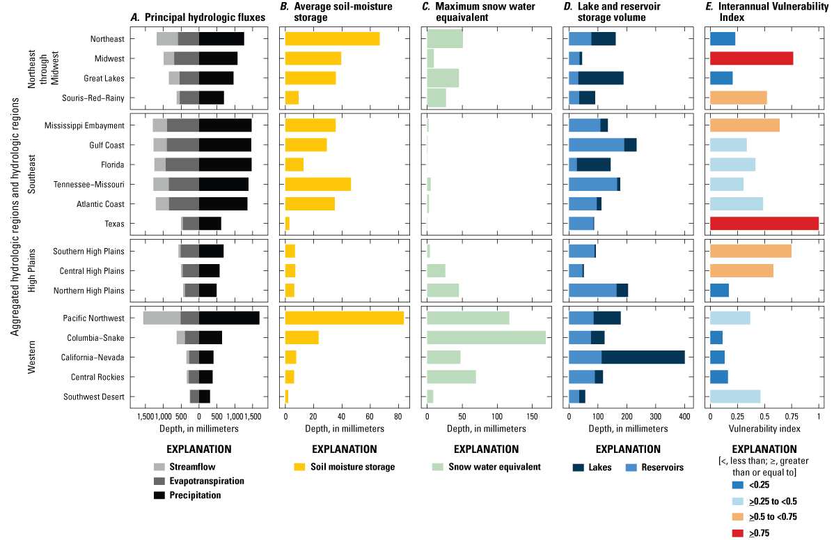
Water budgets summarized by (A) principal hydrologic fluxes (precipitation, streamflow, and evapotranspiration), (B) average soil-moisture storage volume, (C) maximum snow water equivalent, (D) lake and reservoir storage, and (E) Interannual Vulnerability Index, for each hydrologic region and grouped by aggregated hydrologic regions, in the conterminous United States. Interannual Vulnerability Index relates storage volume to precipitation variability, where higher values indicate lower ratio of storage to precipitation variability and therefore higher vulnerability (eq. 2). Precipitation data are from the bias-adjusted 4-kilometer, 40-year long-term regional hydroclimate reanalysis over the conterminous United States (Foks and others, 2024a). Evapotranspiration, streamflow, and snow water equivalent data are ensembled from the National Hydrologic Model Precipitation-Runoff Modeling System (Foks and others, 2024e) and the Weather Research and Forecasting model hydrologic modeling system (Sampson and others, 2024). Soil moisture data are from the National Hydrologic Model Precipitation-Runoff Modeling System (Foks and others, 2024e). Lakes and reservoir data are from the HydroLAKES datasest (Messager and others, 2016).
Areas in which SWE constitutes a large proportion of storage are vulnerable to diminishing storage in the future because of climate change. These areas include the Columbia–Snake, California–Nevada, and the Central Rockies hydrologic regions. This trend is particularly concerning for surface-water supplies in these areas because 53 percent of total streamflow in the Western United States originates from snowmelt and, in mountainous areas, this figure can reach as high as 70 percent (Li and others, 2017). Earlier snowmelt is associated with diminished storage and greater probabilities of unusually low streamflow later in the season. Additionally, more winter precipitation is projected to fall as rain than snow, leading to reduced snowpack and decreased streamflow (chap. E, Scholl and others, 2025).
In the Western and High Plains aggregated hydrologic regions, where precipitation patterns are highly seasonal and show strong interannual variability, storage components serve to buffer water supplies during the dry season and (or) during drier years. In contrast, in the Northeast through Midwest and Southeast aggregated hydrologic regions, which have higher annual precipitation totals than the Western and High Plains aggregated hydrologic regions, storage can contribute considerably to flooding through rain-on-snow events and soil saturation excess (Berghuijs and others, 2016). These events can affect water availability by increasing recharge to groundwater supplies and filling lakes and reservoirs, and negative effects can include degradation of water quality through the mobilization of contaminants.
Uncertainty of Simulated Results
Introduction
The quantification of water fluxes and storage components using CONUS404, NHM–PRMS, and WRF–Hydro (Foks and others, 2024a, 2024b, 2024c, 2024d, 2024e; Sampson and others, 2024), statistical methods for surface-water storage (Messager and others, 2016), and observational data for groundwater storage (U.S. Geological Survey, 2023a) has provided an initial, comprehensive assessment of the national water supply. Although the two hydrologic models, NHM–PRMS and WRF–Hydro, perform well overall (Hay and others, 2023; Rafieeinasab and others, 2024), sources of uncertainty affecting the results are present that need to be considered when using the assessments. Two approaches—benchmarking and d-score comparison of outputs from the two models—were used to quantify uncertainty in the major water-budget components across the CONUS (Martinez and others, 2024). An understanding of the sources and locations of model bias and error can help improve forecasting ability by indicating where better measurements or process representation in the models would reduce uncertainty.
Approach
The uncertainty in the simulated results produced by CONUS404, WRF–Hydro, and NHM–PRMS was estimated by evaluating model forcings and outputs against large, spatially continuous datasets of precipitation, ET, streamflow, SWE, and soil moisture that are representative of the conditions under which the model is used, a process often referred to as benchmarking (Collier and others, 2018). Additionally, model performance was assessed by comparing a suite of benchmark metrics (d-scores) for ET and streamflow simulated by NHM–PRMS and WRF–Hydro to evaluate uncertainty in the ensemble-average results. The datasets chosen for benchmarking also contain uncertainty that is difficult or impossible to measure. However, care was taken to ensure that datasets chosen for comparison purposes:
-
1. were derived from observational measurements (in situ and ex-situ) to model single components of the hydrologic system (for example, Simplified Surface Energy Balance model [SSEBop] estimating ET), and so are not constrained to a balanced water budget;
-
2. have been rigorously compared to other similar datasets in the scientific literature; and
-
3. for the time period of our analysis, had complete spatial coverage across the CONUS.
The comparison to benchmark datasets had two primary goals: (1) to assess the models’ ability to reproduce spatial and temporal patterns observed in benchmark datasets and (2) to identify locations and time periods with strong model overlap and (or) strong model disagreement among models presented and between models and benchmark datasets. Model-estimated storage components and fluxes were compared to benchmarking datasets using the Pearson’s product-moment correlation coefficient (r), the root mean squared error (RMSE), and percent bias (pbias). Although these metrics have their limitations (Legates and McCabe, 1999), r is an easily interpretable metric that facilitates comparison between budget components of different magnitude, RMSE offers an intuitive and widely used metric in the units of the modeled output, and percent bias provides information on systematic model underprediction or overprediction. Error metrics were calculated for each modeling unit (HUC12 for precipitation, ET, and SWE, and 8-digit hydrologic unit code (HUC8) for streamflow and soil moisture) and median values of each metric are presented to summarize model performance across the larger regions or the CONUS. Errors are assessed annually; seasonally as autumn (September, October, November), winter (December, January, February), spring (March, April, May) and summer (June, July, August); and monthly. For assessing the uncertainty of SWE, the annual maximum SWE is compared to the benchmarking dataset.
Additionally, benchmark evaluation of the simulation of evapotranspiration and streamflow was calculated using d-score, which is a novel method to decompose error into two sets of interpretable, orthogonal components: (1) bias, trend, seasonality, and residual; and (2) low, below average, above average, and high. d-score facilitates an understanding and visualization of the structure of the error, including its spatial structure and which components (for example, seasonality, long-term trend) are contributing to the overall error (Hodson and others, 2021). For the d-score, component and overall error in model simulation results are scored on a scale from 0 (indicating worst performance) to 100 (indicating best performance). Because the scores are scaled, the absolute value of the score has little meaning; however, the utility of the d-score method is that it provides a standardized framework for consistent comparison of models and their error components.
Results
Analysis of the annual CONUS-wide estimates of precipitation from CONUS404 (Foks and others, 2024a), and for evapotranspiration and streamflow from the ensemble of NHM–PRMS and WRF–Hydro (Foks and others, 2024e; Sampson and others, 2024) indicated pbias of <10 percent and r>0.74 across the period of analysis. The calculation of errors at the seasonal scale showed that whereas precipitation had a narrow range of seasonal pbias (–0.4 percent in summer to 4.8 percent in autumn), ET had a very wide range (–26 percent in summer to 152 percent in winter). Streamflow was consistently underestimated across all seasons except autumn (1.1 percent), with the spring having the largest magnitude of percent bias (–16.6 percent). The applications of the models developed for this analysis did not simulate open water ET, which contributes to summer ET underestimates. In winter, a high percentage of bias could be driven by a combination of (1) low ET values (which may inflate percent bias calculations), (2) poor understanding of the separate-component rates (evaporation and transpiration) in different regions, and (3) inexact parameterization of snow processes such as sublimation and accumulation that could be targeted for improvement in the hydrologic models. Similarly, the spatial distributions of errors were skewed for ET, streamflow, and SWE, but less so for precipitation and soil moisture. The error estimates presented in tables 6 and 7 show the median error metrics calculated across all HUC12s in the CONUS. For ET, streamflow, and SWE, median values were r=0.74, 0.76, and 0.76, respectively, and mean values (r=0.67, 0.69, and 0.64, respectively) were lower. For precipitation and soil moisture, median values of r=0.79 and 0.72, respectively, were closer to mean values of r=0.80 and 0.72, respectively. These numbers suggest that the models performed well in most HUC12s, whereas a few HUC12s had relatively poor performance.
Table 6.
Uncertainty metrics for annual and seasonal simulated fluxes across the conterminous United States.[See table 1.1 for details on the benchmarking datasets for each water-budget (flux and storage) component. See table 7 for hydrologic region metrics. General interpretation of individual error metrics is as follows: High r value, low RMSE, and low (either positive or negative) bias values represent better model performance. Statistic: r, Pearson’s product-moment correlation coefficient; RMSE, root mean square error; pbias, percent bias. Symbol: —, seasonal metrics not calculated. Precipitation data are from the bias-adjusted 4-kilometer, 40-year long-term regional hydroclimate reanalysis over the conterminous United States (Foks and others, 2024a). Evapotranspiration, streamflow, snow water equivalent, and soil-moisture percent saturation data are ensembled from the National Hydrologic Model Precipitation-Runoff Modeling System (Foks and others, 2024e) and the Weather Research and Forecasting model hydrologic modeling system (Sampson and others, 2024)]
Table 7.
Uncertainty metrics for simulated flux and storage components calculated for each hydrologic region and the conterminous United States.[Snow water equivalent (SWE) error is only shown for hydrologic regions where average maximum SWE is greater than 1 millimeter per year. Abbreviations and symbol: CONUS, conterminous United States; r, Pearson’s product-moment correlation coefficient; RMSE, root mean square error; pbias, percent bias; —, average maximum SWE below threshold data given. Precipitation data are from the bias-adjusted 4-kilometer, 40-year long-term regional hydroclimate reanalysis over the conterminous United States (Foks and others, 2024a). Evapotranspiration, streamflow, snow water equivalent, and soil-moisture percent saturation data are ensembled from the National Hydrologic Model Precipitation-Runoff Modeling System (Foks and others, 2024c) and the Weather Research and Forecasting model hydrologic modeling system (Sampson and others, 2024)]
The overall accuracy of the two hydrologic models in simulating ET was compared using the total d-score, which revealed that WRF–Hydro simulated ET more accurately, with a total score of 93, compared to NHM–PRMS with a total score of 85 (fig. 20A). The d-score method allows the quantitative comparison of error components to enable the further understanding of areas of modeling strength and weakness. For example, WRF–Hydro scored higher than NHM–PRMS on bias (86 compared to 80, respectively) and seasonality (90 compared to 73, respectively), indicating that WRF–Hydro does better simulating the long-term average and seasonal ET pattern than NHM–PRMS (fig. 20A). Additionally, whereas both models do well simulating low-ET periods (winter), WRF–Hydro scores much higher than NHM–PRMS for high-ET periods (summer; 84 for WRF–Hydro and 66 for NHM–PRMS). Figure 20D–20K shows the spatial distribution of a selection of the error-component scores indicating that both models had the lowest performance in Texas and the Gulf Coast hydrologic regions, particularly during summer (shown by low scores during high-ET time periods; fig. 20J, 20K). Evapotranspiration moves a substantial amount of water from the land to the atmosphere, driving the water cycle. The ET-derived water vapor becomes a source of downwind precipitation and controls atmospheric demand for crops and effective temperature (wind chill, heat index). The differences in model performance for ET simulation stem from the more detailed representation of land-atmosphere interactions in WRF–Hydro than in NHM–PRMS; WRF–Hydro has a land-surface model included whereas NHM–PRMS determines ET based on mean daily parameters. Additionally, neither model includes ET that is supplied by groundwater, which can be a substantial flux in some areas (Beamer and others, 2013). Improving the predictive capability of hydrological models requires better understanding of the sensitivity of the models to factors that influence ET and accurate integration of linked processes in the models. This assessment presents an overview of the results; looking further into the component d-scores for subregions can provide more detail on specific factors causing regional uncertainty in simulated ET.
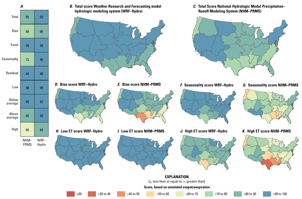
Scorecard and maps showing comparison of the Weather Research and Forecasting model hydrologic modeling system (WRF–Hydro; Sampson and others, 2024) and the National Hydrologic Model Precipitation-Runoff Modeling System (NHM–PRMS; Foks and others, 2024e) simulated evapotranspiration (ET), using the d-score method, across the conterminous United States. (A) Scorecard for the complete error decomposition for entire the conterminous United States. (B–C) Maps showing, for each model, the spatial distribution of the total score. (D–K) Maps showing four components—bias, seasonality, low ET, and high ET. Dark gray lines in maps indicate boundaries between hydrologic regions.
Comparison of the two models’ performance in streamflow simulations using the d-score method showed overall similarity, with total scores of 82 across the CONUS for each model (fig. 21A). Although NHM–PRMS performed better during low-flow periods (d-score of 80 and 77 for NHM–PRMS and WRF–Hydro, respectively), WRF–Hydro performed better during high-flow periods (d-score of 82 and 87 for NHM–PRMS and WRF–Hydro, respectively). Both models captured the trend, seasonality, and residual components of the streamflow benchmarking dataset accurately, but they both had lower accuracy in representing the long-term mean system behavior, as represented by the bias component of the d-score (fig. 21D, 21E). This pattern was particularly apparent in the southwestern parts of the CONUS and High Plains aggregated hydrologic regions, where both models had low bias d-scores. Streamflow in the wetter regions of the country generally was well-represented by both models, as evidenced by the high d-scores across all error components in the Northeast, Great Lakes, and Pacific Northwest hydrologic regions.
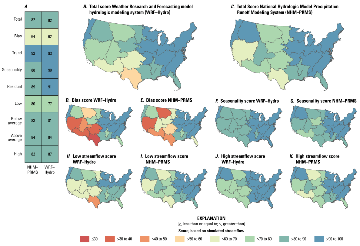
Scorecard and maps showing comparison of the Weather Research and Forecasting model hydrologic modeling system (WRF–Hydro; Sampson and others, 2024) and the National Hydrologic Model Precipitation-Runoff Modeling System (NHM–PRMS; Foks and others, 2024e) simulated streamflow using the d-score method, across the conterminous United States. (A) Scorecard for the complete error decomposition for all of the conterminous United States. (B–C) Maps showing, for each model, the spatial distribution of the total score. (D–K) Maps showing four components—bias, seasonality, low streamflow, and high streamflow. Dark gray lines in maps indicate boundaries between hydrologic regions.
The combination of d-scores (figs. 20 and 21) with traditional error metrics shown in tables 6 and 7 can be used to identify locations and time periods where there is likely inaccurate hydrologic partitioning by the models. For example, in the Texas hydrologic region, both models scored poorly during high-ET time periods (fig. 20J, 20K), and both models scored poorly for streamflow bias (fig. 21D, 21E). In that hydrologic region, ET was underestimated, and streamflow was overestimated, as shown by the percent biases of –30.8 and +93 percent, respectively (table 7). These results indicate that in the Texas hydrologic region, both models’ partitioning schemes overestimated streamflow, particularly during high-ET periods (summer), resulting in large percent biases and low d-scores for high-ET time periods. This result points to several avenues for model improvement, including better representation of the soil-moisture balance and human water use as an input in addition to precipitation, as large amounts of summer irrigation that increase ET are not included in either model. An additional consideration for arid regions and watersheds with high-permeability, geologic substrate is that neither model currently simulates ephemeral streams that have seasonal flow or conditions when streams are losing flow to the aquifer beneath.
For this report, we have presented the ensemble of two operational hydrologic models available at CONUS scale, whose outputs were averaged at the HUC12 monthly scale (Foks and others, 2024e; Sampson and others, 2024). In general, the goal of presenting model ensembles is to provide a range of different representations of the physical processes to generate a distribution of results that is likely to contain the true values and also provide a representation of uncertainty. With any method that involves averaging ensemble results, there is a risk that a single model’s accuracy at a certain time and place may be diluted by other model simulations, leading to a less accurate result. However, this loss of local accuracy will be outweighed by a gain in global accuracy. With the two members of our ensemble, we have used the d-score method to show that, although there are differences in aspects of performance, neither model diverges drastically in performance across the CONUS for streamflow and ET, the two largest hydrologic outputs. Although the detailed analysis of model results for specific periods and locations (where one model outperforms the other) is beyond the scope of this assessment, one of the strengths of the assessment approach that USGS has developed is that this type of analysis can be implemented at a range of spatial and temporal scales, depending on the particular region, river basin, or watershed of interest.
Summary
We present an assessment of water supply across the conterminous United States (CONUS), Alaska, Hawaii, and Puerto Rico covering water years 2010–20 using state-of-the-art hydrologic models at high spatial and temporal resolution. The models simulated the principal hydrologic fluxes (precipitation, evapotranspiration, and streamflow) and storage components (soil moisture and snow water equivalent) are presented at the monthly time step for each 12-digit hydrologic unit code (HUC12). Two additional water-storage components were assessed using other methods—lake and reservoir storage was quantified using a geostatistical modeling approach developed in previous studies (Messager and others, 2016), and the status of groundwater resources was assessed through the analysis of groundwater-level observations in principal and regional aquifers throughout the CONUS.
Results showed that average annual rainfall across the CONUS was 857 millimeters per year (mm/yr) for the period of analysis, with water year 2012 the driest (729 millimeters [mm]) and water year 2019 the wettest (995 mm). Evapotranspiration accounted for an average of 63 percent of precipitation, averaging 539 mm/yr, whereas streamflow accounted for 27 percent, averaging 231 mm/yr . Estimates were characterized by considerable spatial and temporal variability including a severe drought during 2011–12 that resulted in reduced streamflow, evaporation, and soil moisture across much of the High Plains and Northeast through Midwest aggregated hydrologic regions of the country. An analysis of interannual variability revealed that the California–Nevada hydrologic region had the highest variability in precipitation and snow accumulation and that the Texas hydrologic region was among hydrologic regions with the highest variability in precipitation
Our analysis of storage components showed that storage in lakes and reservoirs had highly skewed distributions, with relatively small areas accounting for disproportionately large fractions of storage; for example, the top 1 percent of lakes and reservoirs by volume constituted 99 percent of the total storage in lakes and reservoirs. This pattern highlights the importance of relatively few waterbodies for water supply. Surface-water storage is dominated by the volume of the five Great Lakes, but the Alaska and California–Nevada hydrologic regions and several hydrologic regions throughout the Western and Great Plains aggregated hydrologic regions show high storage volumes in lakes and reservoirs and snowpack. The sum of the three major storage components (soil moisture, lakes and reservoirs, and snow water equivalent) as a percentage of annual precipitation shows that the average combined storage across the conterminous United States was 24 percent, with the Midwest hydrologic region having the lowest percentage (8.5 percent) and the California–Nevada hydrologic region having the highest percentage (110 percent), largely attributable to storage in lakes and reservoirs. Mountainous hydrologic regions in the western CONUS such as the Columbia–Snake, California–Nevada, and Central Rockies, have a large fraction of storage in snow water equivalent, making these areas particularly vulnerable to diminished storage attributable to climate change.
We quantified the relation between interannual variability in precipitation and combined storage volumes to highlight hydrologic regions with interannual vulnerability. The combination of low precipitation and little annually renewable storage in soil moisture, snow, or lakes and reservoirs is a condition where water-availability concerns are likely to emerge or are already prevalent. These areas included the Midwest, Texas, Souris–Red–Rainy, Mississippi Embayment, the Southern High Plains, and Central High Plains hydrologic regions. High interannual vulnerability indicates reduced capacity to withstand variability in precipitation conditions, which could result in increased risk of flooding and (or) decreased ability to store water for later use when precipitation and supplies are low. In many of these regions, groundwater supply fills this need through pumping from regionally important and productive aquifer systems, but an overreliance on slowly recharged groundwater resources has resulted in substantially lowered water levels, particularly in the central and southern regions of the High Plains aquifer, the Rio Grande aquifer system, and the Colorado Plateaus aquifers. Finally, we compared our results to external benchmarking datasets to assess the uncertainty in our estimates of water-budget components, showing that both hydrologic models reproduced patterns in the principal hydrologic fluxes and storage components with high accuracy.
References Cited
Abatzoglou, J.T., 2013, Development of gridded surface meteorological data for ecological applications and modelling: International Journal of Climatology, v. 33, no. 1, p. 121–131, accessed June 24, 2024, at https://doi.org/10.1002/joc.3413.
Abbott, B.W., Bishop, K., Zarnetske, J.P., Minaudo, C., Chapin, F.S., Krause, S., Hannah, D.M., Conner, L., Ellison, D., Godsey, S.E., Plont, S., Marçais, J., Kolbe, T., Huebner, A., Frei, R.J., Hampton, T., Gu, S., Buhman, M., Sara Sayedi, S., Ursache, O., Chapin, M., Henderson, K.D., and Pinay, G., 2019, Human domination of the global water cycle absent from depictions and perceptions: Nature Geoscience, v. 12, no. 7, p. 533–540, accessed October 2, 2023, at https://doi.org/10.1038/s41561-019-0374-y.
Alam, S., Gebremichael, M., Li, R., Dozier, J., and Lettenmaier, D.P., 2020, Can managed aquifer recharge mitigate the groundwater overdraft in California's Central Valley?: Water Resources Research, v. 56, no. 8, 20 p., accessed October 2, 2023, at https://agupubs.onlinelibrary.wiley.com/doi/10.1029/2020WR027244.
Alattar, M.H., Troy, T.J., Russo, T.A., and Boyce, S.E., 2020, Modeling the surface water and groundwater budgets of the US using MODFLOW-OWHM: Advances in Water Resources, v. 143, 27 p., accessed October 2, 2023, at https://doi.org/10.1016/j.advwatres.2020.103682.
Ali, A.A., Tran, D.Q., Kovacs, K.F., and Dahlke, H.E., 2023, Hydro-economic modeling of managed aquifer recharge in the lower Mississippi: Journal of the American Water Resources Association, v. 59, no. 6, p. 1413–1434, accessed April 16, 2023, at https://doi.org/10.1111/1752-1688.13141.
Alley, W.M., 2007, Another water budget myth—The significance of recoverable ground water in storage: Groundwater, v. 45, no. 3, p. 251, accessed October 2, 2023, at https://doi.org/10.1111/j.1745-6584.2006.00274.x.
Alley, W.M., Clark, B.R., Ely, D.M., and Faunt, C.C., 2018, Groundwater development stress—Global-scale indices compared to regional modeling: Ground Water, v. 56, no. 2, p. 266–275, accessed October 2, 2023, at https://doi.org/10.1111/gwat.12578.
Anagnostou, E., Maggioni, V., Nikolopoulos, E., Meskele, T., Hossain, F., and Papadopoulos, A., 2010, Benchmarking high-resolution global satellite rainfall products to radar and rain-gauge rainfall estimates: IEEE Transactions on Geoscience and Remote Sensing, v. 48, no. 4, p. 1667–1683, accessed April 16, 2023, at https://doi.org/10.1109/TGRS.2009.2034736.
Ayers, J.R., Villarini, G., Schilling, K., Jones, C., Brookfield, A., Zipper, S.C., and Farmer, W.H., 2022, The role of climate in monthly baseflow changes across the continental United States: Journal of Hydrologic Engineering, v. 27, no. 5, 13 p., accessed April 16, 2023, at https://doi.org/10.1061/(ASCE)HE.1943-5584.0002170.
Babaeian, E., Sadeghi, M., Jones, S.B., Montzka, C., Vereecken, H., and Tuller, M., 2019, Ground, proximal, and satellite remote sensing of soil moisture: Reviews of Geophysics, v. 57, no. 2, p. 530–616, accessed October 2, 2023, at https://doi.org/10.1029/2018RG000618.
Bales, R.C., Molotch, N.P., Painter, T.H., Dettinger, M.D., Rice, R., and Dozier, J., 2006, Mountain hydrology of the western United States: Water Resources Research, v. 42, no. 8., accessed October 2, 2023, at https://doi.org/10.1029/2005WR004387.
Beamer, J.P., Huntington, J.L., Morton, C.G., and Pohll, G.M., 2013, Estimating annual groundwater evapotranspiration from phreatophytes in the Great Basin using Landsat and flux tower measurements: Journal of the American Water Resources Association, v. 49, no. 3, p. 518–533, accessed April 16, 2023, at https://doi.org/10.1111/jawr.12058.
Belitz, K., Watson, E., Johnson, T.D., and Sharpe, J., 2019, Secondary hydrogeologic regions of the conterminous United States: Groundwater, v. 57, no. 3, p. 367–377, accessed October 2, 2023, at https://doi.org/10.1111/gwat.12806.
Bell, J.E., Leeper, R.D., Palecki, M.A., Coopersmith, E., Wilson, T., Bilotta, R., and Embler, S., 2015, Evaluation of the 2012 drought with a newly established National soil monitoring network: Vadose Zone Journal, v. 14, no. 11, p. 1–7, accessed April 16, 2023, at https://doi.org/10.2136/vzj2015.02.0023.
Berghuijs, W.R., Woods, R.A., Hutton, C.J., and Sivapalan, M., 2016, Dominant flood generating mechanisms across the United States: Geophysical Research Letters, v. 43, no. 9, p. 4382–4390, accessed October 2, 2023, at https://doi.org/10.1002/2016GL068070.
Brookfield, A.E., Zipper, S., Kendall, A.D., Ajami, H., and Deines, J.M., 2024, Estimating groundwater pumping for irrigation—A method comparison: Groundwater, v. 62, no. 1, p. 15–33, accessed October 2, 2023, at https://doi.org/10.1111/gwat.13336.
Brosius, L.S., Anthony, K.M.W., Treat, C.C., Lenz, J., Jones, M.C., Bret-Harte, M.S., and Grosse, G., 2021, Spatiotemporal patterns of northern lake formation since the Last Glacial Maximum: Quaternary Science Reviews, v. 253, 12 p., accessed April 16, 2023, at https://doi.org/10.1016/j.quascirev.2020.106773.
Campbell, B.G., and Coes, A.L., 2010, Groundwater availability in the Atlantic coastal plain of North and South Carolina: U.S. Geological Survey Professional Paper 1773, 240 p., accessed October 2, 2023, at https://doi.org/10.3133/pp1773.
Campisano, A., Butler, D., Ward, S., Burns, M.J., Friedler, E., DeBusk, K., Fisher-Jeffes, L.N., Ghisi, E., Rahman, A., Furumai, H., and Han, M., 2017, Urban rainwater harvesting systems–Research, implementation and future perspectives: Water Research, v. 115, p. 195–209, accessed April 16, 2023, at https://doi.org/10.1016/j.watres.2017.02.056.
Carroll, T., Cline, D., Olheiser, C., Rost, A., Nilsson, A., Fall, G., Bovitz, C., and Li, L., 2006, NOAA’s national snow analyses: Presented at the 74th annual meeting of the Western Snow Conference, National Operational Hydrologic Remote Sensing Center, National Weather Service, National Oceanic and Atmospheric Administration, 14 p., accessed October 2, 2023, at https://www.nohrsc.noaa.gov/technology/pdf/WSC_2006.pdf.
Chahine, M., 1992, The hydrological cycle and its influence on climate: Nature, v. 359, no. 6394, p. 373–380, accessed April 16, 2023, at https://doi.org/10.1038/359373a0.
Cole, J.J., Prairie, Y.T., Caraco, N.F., McDowell, W.H., Tranvik, L.J., Striegl, R.G., Duarte, C.M., Kortelainen, P., Downing, J.A., Middelburg, J.J., and Melack, J., 2007, Plumbing the global carbon cycle—Integrating inland waters into the terrestrial carbon budget: Ecosystems, v. 10, no. 1, p. 172–185, accessed October 2, 2023, at https://doi.org/10.1007/s10021-006-9013-8.
Collier, N., Hoffman, F.M., Lawrence, D.M., Keppel-Aleks, G., Koven, C.D., Riley, W.J., Mu, M., and Randerson, J.T., 2018, The International Land Model Benchmarking (ILAMB) system—Design, theory, and implementation: Journal of Advances in Modeling Earth Systems, v. 10, no. 11, p. 2731–2754, accessed October 2, 2023, at https://doi.org/10.1029/2018MS001354.
Cook, P.G., and Bohlke, J.K., 2000, Determining timescales for groundwater flow and solute transport, in Cook, P.G., and Herczeg, A.L., eds., Environmental tracers in subsurface hydrology: New York, Springer, p. 1–30, accessed April 16, 2023, at https://doi.org/10.1007/978-1-4615-4557-6_1.
Crow, W.T., Chen, F., Reichle, R.H., Xia, Y., and Liu, Q., 2018, Exploiting soil moisture, precipitation, and streamflow observations to evaluate soil moisture/runoff coupling in land surface models: Geophysical Research Letters, v. 45, no. 10, p. 4869–4878, accessed April 16, 2023, at https://doi.org/10.1029/2018GL077193.
DeCicco, L., Hirsch, R., Lorenz, D., Watkins, D., and Johnson, M., 2023, dataRetrieval—R packages for discovering and retrieving water data available from U.S. Federal hydrologic web services: U.S. Geological Survey database, accessed October 2, 2023, at https://doi.org/10.5066/P9X4L3GE.
Degnan, J.R., Kauffman, L.J., Erickson, M.L., Belitz, K., and Stackelberg, P.E., 2021, Depth of groundwater used for drinking-water supplies in the United States: U.S. Geological Survey Scientific Investigations Report 2021–5069, 69 p., accessed April 16, 2023, at https://doi.org/10.3133/sir20215069.
Dettinger, M., 2005, Changes in streamflow timing in the western United States in recent decades: U.S. Geological Survey Fact Sheet 2005–3018, 4 p., accessed October 2, 2023, at https://pubs.usgs.gov/fs/2005/3018/pdf/FS2005_3018.pdf.
Dieter, C.A., Maupin, M.A., Caldwell, R.R., Harris, M.A., Ivahnenko, T.I., Lovelace, J.K., Barber, N.L., and Linsey, K.S., 2018, Estimated use of water in the United States in 2015: U.S. Geological Survey Circular 1441, 65 p., accessed April 16, 2023, at https://doi.org/10.3133/cir1441.
Dillon, P., Fernández Escalante, E., Megdal, S.B., and Massmann, G., 2020, Managed aquifer recharge for water resilience: Water, v. 12, no. 7, 11 p., accessed April 16, 2023, at https://doi.org/10.3390/w12071846.
Dorigo, W.A., Gruber, A., De Jeu, R.A.M., Wagner, W., Stacke, T., Loew, A., Albergel, C., Brocca, L., Chung, D., Parinussa, R.M., and Kidd, R., 2015, Evaluation of the ESA CCI soil moisture product using ground-based observations: Remote Sensing of Environment, v. 162, p. 380–395, accessed October 2, 2023, at https://doi.org/10.1016/j.rse.2014.07.023.
Dorigo, W.A., Wagner, W., Albergel, C., Albrecht, F., Balsamo, G., Brocca, L., Chung, D., Ertl, M., Forkel, M., Gruber, A., Haas, E., Hamer, P.D., Hirschi, M., Ikonen, J., De Jeu, R., Kidd, R., Lahoz, W., Liu, Y.Y., Miralles, D., Mistelbauer, T., Nicolai-Shaw, N., Parinussa, R., Pratola, C., Reimer, C., Van Der Schalie, R., Seneviratne, S.I., Smolander, T., and Lecomte, P., 2017, ESA CCI soil moisture for improved Earth system understanding—State-of-the art and future directions: Remote Sensing of Environment, v. 203, p. 185–215, accessed October 2, 2023, at https://doi.org/10.1016/j.rse.2017.07.001.
Drewes, J.E., 2005, Wastewater reclamation and reuse research, in Water encyclopedia: Hoboken, New Jersey, John Wiley and Sons, p. 819–825, accessed October 2, 2023, at https://doi.org/10.1002/047147844X.ww306.
Eke, J., Yusuf, A., Giwa, A., and Sodiq, A., 2020, The global status of desalination—An assessment of current desalination technologies, plants and capacity: Desalination, v. 495, 17 p., accessed October 2, 2023, at https://doi.org/10.1016/j.desal.2020.114633.
Ely, D.M., Burns, E.R., Morgan, D.S., and Vaccaro, J.J., 2014, Numerical simulation of groundwater flow in the Columbia Plateau regional aquifer system, Idaho, Oregon, and Washington: U.S. Geological Survey Scientific Investigations Report 2014–5127, 102 p., accessed January 10, 2024, at https://doi.org/10.3133/sir20145127.
Entekhabi, D., Rodriguez-Iturbe, I., and Castelli, F., 1996, Mutual interaction of soil moisture state and atmospheric processes: Journal of Hydrology, v. 184, no. 1, p. 3–17, accessed January 10, 2024, at https://doi.org/10.1016/0022-1694(95)02965-6.
Erickson, M.L, Miller, O.L, Cashman, J.J., Degnan, J.R., Reddy, J.E., Martinez, A.J., and Azadpour, E., 2025 Status of water-quality conditions in the United States, 2010–20 (ver. 1.1, February 2025), chap. C of U.S. Geological Survey Integrated Water Availability Assessment—2010–20: U.S. Geological Survey Professional Paper 1894–C, 85 p., https://doi.org/10.3133/pp1894C.
Essaid, H.I., and Caldwell, R.R., 2017, Evaluating the impact of irrigation on surface water–groundwater interaction and stream temperature in an agricultural watershed: Science of The Total Environment, v. 599–600, p. 581–596, accessed January 10, 2024, at https://doi.org/10.1016/j.scitotenv.2017.04.205.
Foks, S.S., LaMotte, A.E., LaFontaine, J.H., and Viger, R.J., 2024a, Monthly twelve-digit hydrologic unit code aggregations of the CONUS404 bias adjusted application, 1979–2021: U.S. Geological Survey data release, accessed January 6, 2025, at https://doi.org/10.5066/P1AM8AM7.
Foks, S.S., LaFontaine, J.H., McDonald, R.R., Snyder, A.M., Kolb, K.R., LaMotte, A.E., and Viger, R.J., 2024b, Monthly twelve-digit hydrologic unit code aggregations of the National Hydrologic Model Precipitation-Runoff Modeling System modeling application for Alaska, 1980–2021: U.S. Geological Survey data release, accessed January 6, 2025, at https://doi.org/10.5066/P149Z4G9.
Foks, S.S., LaFontaine, J.H., McDonald, R.R., Snyder, A.M., Kolb, K.R., LaMotte, A.E., and Viger, R.J., 2024c, Monthly twelve-digit hydrologic unit code aggregations of the National Hydrologic Model Precipitation-Runoff Modeling System modeling application for Hawaii, 1980–2021: U.S. Geological Survey data release, accessed January 6, 2025, at https://doi.org/10.5066/P14NFNOJ.
Foks, S.S., LaFontaine, J.H., McDonald, R.R., Snyder, A.M., Kolb, K.R., LaMotte, A.E., and Viger, R.J., 2024d, Monthly twelve-digit hydrologic unit code aggregations of the National Hydrologic Model Precipitation-Runoff Modeling System modeling application for Puerto Rico, 1950–2021: U.S. Geological Survey data release, accessed January 6, 2025, at https://doi.org/10.5066/P1ERNH5C.
Foks, S.S., LaFontaine, J.H., McDonald, R.M., Synder, A.M., Staub, L.E., Kolb, K., LaMotte, A.E., and Viger, R.J., 2024e, Monthly twelve-digit hydrologic unit code aggregations of the National Hydrologic Model Precipitation-Runoff Modeling System version 1.1 forced with CONUS404-BA, 1980–2021: U.S. Geological Survey data release, accessed January 6, 2025, at https://doi.org/10.5066/P14C5YAP.
Gaur, N., and Mohanty, B.P., 2013, Evolution of physical controls for soil moisture in humid and subhumid watersheds: Water Resources Research, v. 49, no. 3, p. 1244–1258, accessed January 10, 2024, at https://doi.org/10.1002/wrcr.20069.
Gleason, C.J., and Durand, M.T., 2020, Remote sensing of river discharge—A review and a framing for the discipline: Remote Sensing, v. 12, no. 7, 28 p., accessed October 2, 2023, at https://doi.org/10.3390/rs12071107.
Global Energy and Water Exchanges, 2012, GEWEX Plans for 2013 and beyond—Imperatives (version 1): GEWEX, 49 p., accessed October 2, 2023, at http://www.gewex.org/gewex-content/uploads/2015/02/GEWEX_Imperatives_final.pdf.
Gochis, D.J., Barlage, M., Cabell, R., Casali, M., Dugger, A., FitzGerald, K., McAllister, M., and McCreight, J., Rafieeinasab, A., Read, L., Sampson, K., Yates, D., and Zhang, Y., 2020, The WRF–Hydro modeling system technical description: National Science Foundation National Center for Atmospheric Research NCAR Technical Note (version 5.1.1.), accessed October 2, 2023, at https://ral.ucar.edu/projects/wrf_hydro/documentation/WRF–Hydro-v511-documentation.
Godsey, S.E., Kirchner, J.W., and Tague, C.L., 2014, Effects of changes in winter snowpacks on summer low flows—Case studies in the Sierra Nevada, California, USA: Hydrological Processes, v. 28, no. 19, p. 5048–5064, accessed January 10, 2024, at https://doi.org/10.1002/hyp.9943.
Hammond, J.C., Saavedra, F.A., and Kampf, S.K., 2018, How does snow persistence relate to annual streamflow in mountain watersheds of the western U.S. with wet maritime and dry continental climates?: Water Resources Research, v. 54, no. 4, p. 2605–2623, accessed October 2, 2023, at https://doi.org/10.1002/2017WR021899.
Hanasaki, N., Yoshikawa, S., Kakinuma, K., and Kanae, S., 2016, A seawater desalination scheme for global hydrological models: Hydrology and Earth System Sciences, v. 20, no. 10, p. 4143–4157, accessed October 2, 2023, at https://doi.org/10.5194/hess-20-4143-2016.
Harbaugh, A.W., 2005, MODFLOW-2005—The U.S. Geological Survey modular ground-water model—The ground-water flow process: U.S. Geological Survey Techniques and Methods, book 6, chap. A16, accessed January 10, 2024, at https://doi.org/10.3133/tm6A16.
Harpold, A.A., Sutcliffe, K., Clayton, J., Goodbody, A., and Vazquez, S., 2017, Does including soil moisture observations improve operational streamflow forecasts in snow-dominated watersheds?: Journal of the American Water Resources Association, v. 53, no. 1, p. 179–196, accessed October 2, 2023, at https://doi.org/10.1111/1752-1688.12490.
Harvey, J.W., and Schmadel, N.M., 2021, The river corridor’s evolving connectivity of lotic and lentic waters: Frontiers in Water, v. 2, 17 p., accessed October 2, 2023, at https://www.frontiersin.org/journals/water/articles/10.3389/frwa.2020.580727.
Hay, L.E., LaFontaine, J.H., Van Beusekom, A.E., Norton, P.A., Farmer, W.H., Regan, R.S., Markstrom, S.L., and Dickinson, J.E., 2023, Parameter estimation at the conterminous United States scale and streamflow routing enhancements for the National Hydrologic Model infrastructure application of the Precipitation-Runoff Modeling System (NHM–PRMS): U.S. Geological Survey Techniques and Methods, book 6, chap. B10, 50 p., accessed October 2, 2023, at https://doi.org/10.3133/tm6B10.
Healy, R.W., 2010, Estimating groundwater recharge: Cambridge, United Kingdom, Cambridge University Press, 245 p. [Also available at https://doi.org/10.1017/CBO9780511780745.]
Henn, B., Musselman, K.N., Lestak, L., Ralph, F.M., and Molotch, N.P., 2020, Extreme runoff generation from atmospheric river driven snowmelt during the 2017 Oroville Dam spillways incident: Geophysical Research Letters, v. 47, no. 14, 11 p., accessed October 2, 2023, at https://doi.org/10.1029/2020GL088189.
Hobeichi, S., Abramowitz, G., and Evans, J., 2020, Conserving Land–Atmosphere Synthesis Suite (CLASS): Journal of Climate, v. 33, no. 5, p. 1821–1844, accessed October 2, 2023, at https://doi.org/10.1175/JCLI-D-19-0036.1.
Hodson, T.O., Over, T.M., and Foks, S.S., 2021, Mean squared error, deconstructed: Journal of Advances in Modeling Earth Systems, v. 13, no. 12, 10 p., accessed October 2, 2023, at https://doi.org/10.1029/2021MS002681.
Hoerling, M., Eischeid, J., Kumar, A., Leung, R., Mariotti, A., Mo, K., Schubert, S., and Seager, R., 2014, Causes and predictability of the 2012 Great Plains drought: Bulletin of the American Meteorological Society, v. 95, no. 2, p. 269–282, accessed October 2, 2023, at https://doi.org/10.1175/BAMS-D-13-00055.1.
Jakeman, A.J., Barreteau, O., Hunt, R.J., Rinaudo, J.-D., Ross, A., Arshad, M., and Hamilton, S., 2016, Integrated groundwater management—An overview of concepts and challenges, in Jakeman, A.J., Barreteau, O., Hunt, R.J., Rinaudo, J.-D., and Ross, A., eds., Integrated groundwater management—Concepts, approaches and challenges: Cham, Switzerland, Springer International Publishing, p. 3–20, accessed January 10, 2024, at https://doi.org/10.1007/978-3-319-23576-9_1.
Jasechko, S., Seybold, H., Perrone, D., Fan, Y., and Kirchner, J.W., 2021, Widespread potential loss of streamflow into underlying aquifers across the USA: Nature, v. 591, no. 7850, p. 391–395, accessed October 2, 2023, at https://doi.org/10.1038/s41586-021-03311-x.
Kao, S.-C., Ashfaq, M., Rastogi, D., Gangrade, S., Uria Martinez, R., Fernandez, A., Konapala, G., Voisin, N., Zhou, T., Xu, W., Gao, H., Zhao, B., and Zhao, G., 2022, The third assessment of the effects of climate change on Federal hydropower: Oak Ridge National Laboratory Technical Report ORNL/TM-2021/2278, 310 p., accessed October 2, 2023, at https://doi.org/10.2172/1887712.
Konikow, L.F., 2013, Groundwater depletion in the United States (1900–2008): U.S. Geological Survey Scientific Investigations Report 2013–5079, 65 p., accessed October 2, 2023, at https://doi.org/10.3133/sir20135079.
Koster, R.D., Mahanama, S.P.P., Livneh, B., Lettenmaier, D.P., and Reichle, R.H., 2010, Skill in streamflow forecasts derived from large-scale estimates of soil moisture and snow: Nature Geoscience, v. 3, no. 9, p. 613–616, accessed January 10, 2024, at https://doi.org/10.1038/ngeo944.
Lahnsteiner, J., van Rensburg, P., and Esterhuizen, J., 2017, Direct potable reuse—A feasible water management option: Journal of Water Reuse and Desalination, v. 8, no. 1, p. 14–28, accessed January 10, 2024, at https://doi.org/10.2166/wrd.2017.172.
Langevin, C.D., Hughes, J.D., Banta, E.R., Niswonger, R.G., Panday, S., and Provost, A.M., 2017, Documentation for the MODFLOW 6 groundwater flow model: U.S. Geological Survey Techniques and Methods, book 6, chap. A55, 197 p., accessed October 2, 2023, at https://doi.org/10.3133/tm6A55.
L’Ecuyer, T.S., Beaudoing, H.K., Rodell, M., Olson, W., Lin, B., Kato, S., Clayson, C.A., Wood, E., Sheffield, J., Adler, R., Huffman, G., Bosilovich, M., Gu, G., Robertson, F., Houser, P.R., Chambers, D., Famiglietti, J.S., Fetzer, E., Liu, W.T., Gao, X., Schlosser, C.A., Clark, E., Lettenmaier, D.P., and Hilburn, K., 2015, The observed state of the energy budget in the early twenty-first century: Journal of Climate, v. 28, no. 21, p. 8319–8346, accessed October 2, 2023, at https://doi.org/10.1175/JCLI-D-14-00556.1.
Legates, D.R., Mahmood, R., Levia, D.F., DeLiberty, T.L., Quiring, S.M., Houser, C., and Nelson, F.E., 2011, Soil moisture—A central and unifying theme in physical geography—Progress in physical geography: Earth and Environment, v. 35, no. 1, p. 65–86, accessed October 2, 2023, at https://doi.org/10.1177/0309133310386514.
Legates, D.R., and McCabe, Jr., G.J., 1999, Evaluating the use of “goodness-of-fit” measures in hydrologic and hydroclimatic model validation: Water Resources Research, v. 35, no. 1, p. 233–241, accessed October 2, 2023, at https://doi.org/10.1029/1998WR900018.
Lehmann, F., Vishwakarma, B.D., and Bamber, J., 2022, How well are we able to close the water budget at the global scale?: Hydrology and Earth System Sciences, v. 26, no. 1, p. 35–54, accessed October 2, 2023, at https://doi.org/10.5194/hess-26-35-2022.
Lehner, B., Liermann, C.R., Revenga, C., Vörösmarty, C., Fekete, B., Crouzet, P., Döll, P., Endejan, M., Frenken, K., Magome, J., Nilsson, C., Robertson, J.C., Rödel, R., Sindorf, N., and Wisser, D., 2011, High-resolution mapping of the world's reservoirs and dams for sustainable river-flow management: Frontiers in Ecology and the Environment, v. 9, no. 9, p. 494–502, accessed October 2, 2023, at https://doi.org/10.1890/100125.
Lerner, D.N., 1998, Groundwater recharge, in Saether, O.M., and deCaritat, P., eds., Geochemical processes, weathering and groundwater recharge in catchments (1st ed.): London, CRC Press, 400 p., accessed October 2, 2023, at https://doi.org/10.2134/jeq1998.00472425002700060040x.
Li, D., Wrzesien, M.L., Durand, M., Adam, J., and Lettenmaier, D.P., 2017, How much runoff originates as snow in the western United States, and how will that change in the future?: Geophysical Research Letters, v. 44, no. 12, p. 6163–6172, accessed October 2, 2023, at https://doi.org/10.1002/2017GL073551.
Li, M., Wu, P., and Ma, Z., 2020, A comprehensive evaluation of soil moisture and soil temperature from third-generation atmospheric and land reanalysis data sets: International Journal of Climatology, v. 40, no. 13, p. 5744–5766, accessed January 10, 2024, at https://doi.org/10.1002/joc.6549.
Long, D., Scanlon, B.R., Longuevergne, L., Sun, A.Y., Fernando, D.N., and Save, H., 2013, GRACE satellite monitoring of large depletion in water storage in response to the 2011 drought in Texas: Geophysical Research Letters, v. 40, no. 13, p. 3395–3401, accessed January 10, 2024, at https://doi.org/10.1002/grl.50655.
Lovelace, J.K., Nielsen, M.G., Read, A.L., Murphy, C.J., and Maupin, M.A., 2020, Estimated groundwater withdrawals from principal aquifers in the United States: U.S. Geological Survey Circular 1464, 82 p., accessed January 10, 2024, at https://doi.org/10.3133/cir1464.
Magilligan, F.J., and Nislow, K.H., 2005, Changes in hydrologic regime by dams: Geomorphology, v. 71, nos. 1–2, p. 61–78, accessed October 2, 2023, at https://doi.org/10.1016/j.geomorph.2004.08.017.
Mai, J., Craig, J.R., Tolson, B.A., and Arsenault, R., 2022, The sensitivity of simulated streamflow to individual hydrologic processes across North America: Nature Communications, v. 13, no. 1, 11 p., accessed October 2, 2023, at https://doi.org/10.1038/s41467-022-28010-7.
Margulis, S.A., Cortés, G., Girotto, M., Huning, L.S., Li, D., and Durand, M., 2016, Characterizing the extreme 2015 snowpack deficit in the Sierra Nevada (USA) and the implications for drought recovery: Geophysical Research Letters, v. 43, no. 12, p. 6341–6349, accessed January 10, 2024, at https://doi.org/10.1002/2016GL068520.
Martinez, A.J., Padilla, J.A., and Gorski, G., 2024, Monthly ensemble outputs from the National Hydrologic Model Precipitation-Runoff Modeling System and the Weather Research and Forecasting model hydrologic modeling system for the conterminous United States, Alaska, Hawaii, and Puerto Rico for water years 2010–2020: U.S. Geological Survey data release, accessed January 7, 2025, at https://doi.org/10.5066/P1RBMDUT.
Maxwell, R.M., and Condon, L.E., 2016, Connections between groundwater flow and transpiration partitioning: Science, v. 353, no. 6297, p. 377–380, accessed January 10, 2024, at https://doi.org/10.1126/science.aaf7891.
McDonald, C.P., Rover, J.A., Stets, E.G., and Striegl, R.G., 2012, The regional abundance and size distribution of lakes and reservoirs in the United States and implications for estimates of global lake extent: Limnology and Oceanography, v. 57, no. 2, p. 597–606, accessed April 16, 2023, at https://doi.org/10.4319/lo.2012.57.2.0597.
McGuire, V.L., 2013, Water-level and storage changes in the High Plains aquifer, predevelopment to 2011 and 2009–2011: U.S. Geological Survey Scientific Investigations Report 2012–5291, accessed April 16, 2023, at https://pubs.usgs.gov/sir/2012/5291/.
McMahon, P.B., Böhlke, J.K., and Christenson, S.C., 2004, Geochemistry, radiocarbon ages, and paleorecharge conditions along a transect in the central High Plains aquifer, southwestern Kansas, USA: Applied Geochemistry, v. 19, no. 11, p. 1655–1686, accessed January 10, 2024, at https://doi.org/10.1016/j.apgeochem.2004.05.003.
Medalie, L., Galanter, A.E., Martinez, A.J., and Archer, A.A., Luukkonen, C.L., Harris, M.A., and Haynes, J.V., 2025, Water use across the conterminous United States, water years 2010–20, chap. D of U.S. Geological Survey Integrated Water Availability Assessment—2010–20: U.S. Geological Survey Professional Paper 1894–D, 56 p., https://doi.org/10.3133/pp1894D.
Messager, M.L., Lehner, B., Grill, G., Nedeva, I., and Schmitt, O., 2016, Estimating the volume and age of water stored in global lakes using a geo-statistical approach: Nature Communications, v. 7, no. 1, 11 p., accessed October 2, 2023, at https://doi.org/10.1038/ncomms13603.
Milly, P.C.D., and Dunne, K.A., 2016, Potential evapotranspiration and continental drying: Nature Climate Change, v. 6, no. 10, p. 946–949, accessed April 16, 2023, at https://doi.org/10.1038/nclimate3046.
Myers, N.C., 2022, Composite regional groundwater hydrographs for selected principal aquifers in New Mexico, 1980–2019: U.S. Geological Survey Open-File Report 2022–1008, 64 p., accessed January 10, 2024, at https://doi.org/10.3133/ofr20221008.
Nace, R.L., 1969, World water inventory and control 1, in Introduction to geographical hydrology: New York, Routledge, 12 p., accessed January 10, 2024, at https://www.taylorfrancis.com/chapters/edit/10.4324/9780429273322-2/world-water-inventory-control-1-nace.
Pi, X., Luo, Q., Feng, L., Xu, Y., Tang, J., Liang, X., Ma, E., Cheng, R., Fensholt, R., Brandt, M., Cai, X., Gibson, L., Liu, J., Zheng, C., Li, W., and Bryan, B.A., 2022, Mapping global lake dynamics reveals the emerging roles of small lakes: Nature Communications, v. 13, no. 1, 12 p., accessed January 10, 2024, at https://doi.org/10.1038/s41467-022-33239-3.
Qiu, J., Crow, W.T., and Nearing, G.S., 2016, The impact of vertical measurement depth on the information content of soil moisture for latent heat flux estimation: Journal of Hydrometeorology, v. 17, no. 9, p. 2419–2430, accessed April 16, 2023, at https://doi.org/10.1175/JHM-D-16-0044.1.
Rafieeinasab, A., Dugger, A., Mazrooei, A., Enzminger, T., Srivatava, I., Gochis, D., Sampson, K., Omani, N., Grim, J., Zhang, Y., LaFontaine, J., Viger, R., Liu, Y., and Schneider, T., 2024, A WRF–Hydro-based retrospective simulation of water resources for US integrated water availability assessment: Hydrology and Earth System Sciences Discussions, 37 p., accessed December 15, 2024, at https://doi.org/10.5194/hess-2024-262.
Rasmussen, R.M., Chen, F., Liu, C.H., Ikeda, K., Prein, A., Kim, J., Schneider, T., Dai, A., Gochis, D., Dugger, A., Zhang, Y., Jaye, A., Dudhia, J., He, C., Harrold, M., Xue, L., Chen, S., Newman, A., Dougherty, E., Abolafia-Rosenzweig, R., Lybarger, N.D., Viger, R., Lesmes, D., Skalak, K., Brakebill, J., Cline, D., Dunne, K., Rasmussen, K., and Miguez-Macho, G., 2023, CONUS404—The NCAR–USGS 4-km long-term regional hydroclimate reanalysis over the CONUS: Bulletin of the American Meteorological Society, v. 104, no. 8, p. E1382–E1408, accessed April 16, 2023, at https://doi.org/10.1175/BAMS-D-21-0326.1.
Rateb, A., Scanlon, B.R., Pool, D.R., Sun, A., Zhang, Z., Chen, J., Clark, B., Faunt, C.C., Haugh, C.J., Hill, M., Hobza, C., McGuire, V.L., Reitz, M., Müller Schmied, H., Sutanudjaja, E.H., Swenson, S., Wiese, D., Xia, Y., and Zell, W., 2020, Comparison of groundwater storage changes from GRACE satellites with monitoring and modeling of major U.S. aquifers: Water Resources Research, v. 56, no. 12, 19 p., accessed April 16, 2023, at https://doi.org/10.1029/2020WR027556.
Regan, R.S., Juracek, K.E., Hay, L.E., Markstrom, S.L., Viger, R.J., Driscoll, J.M., LaFontaine, J.H., and Norton, P.A., 2019, The U.S. Geological Survey National Hydrologic Model infrastructure—Rationale, description, and application of a watershed-scale model for the conterminous United States: Environmental Modelling & Software, v. 111, p. 192–203, accessed April 16, 2024, at https://doi.org/10.1016/j.envsoft.2018.09.023.
Regan, R.S., Markstrom, S.L., Hay, L.E., Viger, R.J., Norton, P.A., Driscoll, J.M., and LaFontaine, J.H., 2018, Description of the National Hydrologic Model for use with the Precipitation-Runoff Modeling System (PRMS): U.S. Geological Survey Techniques and Methods, book 6, chap. B9, 38 p., accessed October 2, 2023, at https://doi.org/10.3133/tm6B9.
Reilly, T.E., Dennehy, K.F., Alley, W.M., and Cunningham, W.L., 2008, Ground-water availability in the United States: U.S. Geological Survey Circular 1323, 70 p., accessed January 10, 2024, at https://doi.org/10.3133/cir1323.
Reitz, M., Sanford, W.E., Senay, G., and Cazenas, J., 2017, Annual estimates of recharge, quick-flow runoff, and ET for the contiguous U.S. using empirical regression equations: Journal of the American Water Resources Association, v. 53, no. 4, p. 961–983, accessed October 2, 2023, at https://doi.org/10.1111/1752-1688.12546.
Rodell, M., Beaudoing, H.K., L’Ecuyer, T.S., Olson, W.S., Famiglietti, J.S., Houser, P.R., Adler, R., Bosilovich, M.G., Clayson, C.A., Chambers, D., Clark, E., Fetzer, E.J., Gao, X., Gu, G., Hilburn, K., Huffman, G.J., Lettenmaier, D.P., Liu, W.T., Robertson, F.R., Schlosser, C.A., Sheffield, J., and Wood, E.F., 2015, The observed state of the water cycle in the early twenty-first century: Journal of Climate, v. 28, no. 21, p. 8289–8318, accessed October 2, 2023, at https://doi.org/10.1175/JCLI-D-14-00555.1.
Rosa, E., Larocque, M., Hatch, C.E., and Springer, A.E., 2023, Editorial—“Novel approaches for understanding groundwater dependent ecosystems in a changing environment”: Frontiers in Earth Science, v. 11, 3 p., accessed April 16, 2023, at https://doi.org/10.3389/feart.2023.1165061.
Russo, T.A., Fisher, A.T., and Lockwood, B.S., 2015, Assessment of managed aquifer recharge site suitability using a GIS and modeling: Ground Water, v. 53, no. 3, p. 389–400, accessed January 10, 2024, at https://doi.org/10.1111/gwat.12213.
Sampson, K., Dugger, A., Rafieeinasab, A., Zhang, Y., LaFontaine, J.H., Foks, S.S., LaMotte, A.E., and Viger, R.J., 2024, Monthly twelve-digit hydrologic unit code aggregations of the WRF–Hydro application with CONUS404BA atmospheric forcings, 2009–2021: U.S. Geological Survey data release, accessed December 15, 2024, at https://doi.org/10.5066/P13QA5KX.
Saunders, K.S., Mayes, K.B., Jurgensen, T.A., Trungale, J.F., Kleinsasser, L.J., Aziz, K., Fields, J.R., and Moss, R.E., 2001, An evaluation of spring flows to support the Upper San Marcos River spring ecosystem: Texas Parks and Wildlife Department River Studies Report 16, 109 p., accessed October 2, 2023, at https://tpwd.texas.gov/publications/pwdpubs/media/pwd_rp_t3200_1087.pdf.
Scanlon, B.R., Faunt, C.C., Longuevergne, L., Reedy, R.C., Alley, W.M., McGuire, V.L., and McMahon, P.B., 2012, Groundwater depletion and sustainability of irrigation in the US High Plains and Central Valley: Proceedings of the National Academy of Sciences, v. 109, no. 24, p. 9320–9325, accessed October 2, 2023, at https://doi.org/10.1073/pnas.1200311109.
Scanlon, B.R., Healy, R.W., and Cook, P.G., 2002, Choosing appropriate techniques for quantifying groundwater recharge: Hydrogeology Journal, v. 10, no. 1, p. 18–39, accessed October 2, 2023, at https://doi.org/10.1007/s10040-001-0176-2.
Scholl, M.A., McCabe, G.J., Olson, C.G., and Powlen, K.A., 2025, Climate change and future water availability in the United States, chap. E of U.S. Geological Survey Integrated Water Availability Assessment—2010–20: U.S. Geological Survey Professional Paper 1894–E, 60 p., https://doi.org/10.3133/pp1894E.
Senay, G.B., 2018, Satellite psychrometric formulation of the operational Simplified Surface Energy Balance (SSEBop) model for quantifying and mapping evapotranspiration: Applied Engineering in Agriculture, v. 34, no. 3, p. 555–566, accessed October 2, 2023, at https://doi.org/10.13031/aea.12614.
Senay, G.B., Bohms, S., Singh, R.K., Gowda, P.H., Velpuri, N.M., Alemu, H., and Verdin, J.P., 2013, Operational evapotranspiration mapping using remote sensing and weather datasets—A new parameterization for the SSEB approach: JAWRA Journal of the American Water Resources Association, v. 49, no. 3, p. 577–591, accessed October 2, 2023, at https://doi.org/10.1111/jawr.12057.
Seneviratne, S.I., Corti, T., Davin, E.L., Hirschi, M., Jaeger, E.B., Lehner, I., Orlowsky, B., and Teuling, A.J., 2010, Investigating soil moisture–climate interactions in a changing climate—A review: Earth-Science Reviews, v. 99, nos. 3–4, p. 125–161, accessed October 2, 2023, at https://doi.org/10.1016/j.earscirev.2010.02.004.
Sexstone, G.A., Driscoll, J.M., Hay, L.E., Hammond, J.C., and Barnhart, T.B., 2020, Runoff sensitivity to snow depletion curve representation within a continental scale hydrologic model: Hydrological Processes, v. 34, no. 11, p. 2365–2380, accessed April 16, 2023, at https://doi.org/10.1002/hyp.13735.
Siddik, M.A.B., Dickson, K.E., Rising, J., Ruddell, B.L., and Marston, L.T., 2023, Interbasin water transfers in the United States and Canada: Scientific Data, v. 10, no. 1, 9 p., accessed January 10, 2024, at https://doi.org/10.1038/s41597-023-01935-4.
Siirila-Woodburn, E.R., Rhoades, A.M., Hatchett, B.J., Huning, L.S., Szinai, J., Tague, C., Nico, P.S., Feldman, D.R., Jones, A.D., Collins, W.D., and Kaatz, L., 2021, A low-to-no snow future and its impacts on water resources in the western United States: Nature Reviews Earth & Environment, v. 2, no. 11, p. 800–819, accessed October 2, 2023, at https://doi.org/10.1038/s43017-021-00219-y.
Singh, G., Kaur, G., Williard, K., Schoonover, J., and Kang, J., 2018, Monitoring of water and solute transport in the vadose zone—A review: Vadose Zone Journal, v. 17, no. 1, 23 p., accessed April 16, 2023, at https://doi.org/10.2136/vzj2016.07.0058.
Smith, A.B., 2023, U.S. billion-dollar weather and climate disasters, 1980–present (NCEI accession 0209268): National Oceanic and Atmospheric Administration, National Centers for Environmental Information dataset, accessed October 2, 2023, at https://doi.org/10.25921/stkw-7w73.
Soller, D.R., Reheis, M.C., Garrity, C.P., and Van Sistine, D.R., 2009, Map database for surficial materials in the conterminous United States: U.S. Geological Survey Data Series 425, scale 1:5,000,000, accessed October 2, 2023, at https://pubs.usgs.gov/ds/425/.
Stanton, J.S., Qi, S.L., Ryter, D.W., Falk, S.E., Houston, N.A., Peterson, S.M., Westenbroek, S.M., and Christenson, S.C., 2011, Selected approaches to estimate water budget components of the High Plains, 1940 through 1949 and 2000 through 2009: U.S. Geological Survey Scientific Investigations Report 2011–5183, 79 p., accessed January 10, 2024, at https://doi.org/10.3133/sir20115183.
Stets, E.G., Archer, A.A., Degnan, J.R., Erickson, M.L., Gorski, G., Medalie, L, and Scholl, M.A., 2025a, The national integrated water availability assessment, water years 2010–20, chap. A of U.S. Geological Survey Integrated Water Availability Assessment—2010–20: U.S. Geological Survey Professional Paper 1894–A, 24 p., https://doi.org/10.3133/pp1894A.
Stets, E.G., Cashman, M.J., Miller, O.L., and Powlen, K.A., 2025b, Integrated water availability in the conterminous United States, 2010–20, chap. F of U.S. Geological Survey Integrated Water Availability Assessment—2010–20: U.S. Geological Survey Professional Paper 1894–F, 41 p., https://doi.org/10.3133/pp1894F.
Tapley, B.D., Watkins, M.M., Flechtner, F., Reigber, C., Bettadpur, S., Rodell, M., Sasgen, I., Famiglietti, J.S., Landerer, F.W., Chambers, D.P., Reager, J.T., Gardner, A.S., Save, H., Ivins, E.R., Swenson, S.C., Boening, C., Dahle, C., Wiese, D.N., Dobslaw, H., Tamisiea, M.E., and Velicogna, I., 2019, Contributions of GRACE to understanding climate change: Nature Climate Change, v. 9, no. 5, p. 358–369, accessed October 2, 2023, at https://doi.org/10.1038/s41558-019-0456-2.
Thornton, M.M., Shrestha, R., Wei, Y., Thornton, P.E., Kao, S.C., and Wilson, B.E., 2022, Daymet—Daily surface weather data on a 1-km grid for North America, version 4 R1: Oak Ridge National Laboratory Distributed Active Archive Center dataset, accessed October 2, 2023, at https://doi.org/10.3334/ORNLDAAC/2129.
Tran, D.Q., and Kovacs, K.F., 2021, Climate uncertainty and optimal groundwater augmentation: Water Resources Research, v. 57, no. 9, 19 p., accessed October 2, 2023, at https://doi.org/10.1029/2021WR030114.
Upper Midwest Water Science Center, 2002, Alluvial and glacial aquifers: U.S. Geological Survey data release, accessed January 10, 2024, at https://doi.org/10.5066/P9QA3WA5.
U.S. Geological Survey, 2000, Ground water atlas of the United States: U.S. Geological Survey Hydrologic Atlas 730, accessed October 2, 2023, at https://doi.org/10.3133/ha730.
U.S. Geological Survey, 2003, Principal aquifers of the 48 conterminous United States, Hawaii, Puerto Rico, and the U.S. Virgin Islands: U.S. Geological Survey data release, accessed January 10, 2024, at https://doi.org/10.5066/P9Y2HOUJ.
U.S. Geological Survey, 2023a, National Groundwater Monitoring Network: U.S. Geological Survey database, accessed April 10, 2023, at https://cida.usgs.gov/ngwmn/.
U.S. Geological Survey, 2023b, Watershed boundary dataset: U.S. Geological Survey dataset, accessed July 27, 2023, at https://www.usgs.gov/national-hydrography/watershed-boundary-dataset.
U.S. Geological Survey, 2023c, WaterWatch: U.S. Geological Survey database, accessed October 2, 2023, at https://waterwatch.usgs.gov/.
Van Metre, P.C., Qi, S., Deacon, J., Dieter, C., Driscoll, J.M., Fienen, M., Kenney, T., Lambert, P., Lesmes, D., Mason, C.A., Mueller-Solger, A., Musgrove, M., Painter, J., Rosenberry, D., Sprague, L., Tesoriero, A.J., Windham-Myers, L., and Wolock, D., 2020, Prioritizing river basins for intensive monitoring and assessment by the U.S. Geological Survey: Environmental Monitoring and Assessment, v. 192, no. 7, 17 p., accessed October 2, 2023, at https://doi.org/10.1007/s10661-020-08403-1.
Vereecken, H., Amelung, W., Bauke, S.L., Bogena, H., Brüggemann, N., Montzka, C., Vanderborght, J., Bechtold, M., Blöschl, G., Carminati, A., Javaux, M., Konings, A.G., Kusche, J., Neuweiler, I., Or, D., Steele-Dunne, S., Verhoef, A., Young, M., and Zhang, Y., 2022, Soil hydrology in the Earth system: Nature Reviews Earth & Environment, v. 3, no. 9, p. 573–587, accessed January 10, 2024, at https://doi.org/10.1038/s43017-022-00324-6.
Vereecken, H., Huisman, J.A., Pachepsky, Y., Montzka, C., van der Kruk, J., Bogena, H., Weihermüller, L., Herbst, M., Martinez, G., and Vanderborght, J., 2014, On the spatio-temporal dynamics of soil moisture at the field scale: Journal of Hydrology, v. 516, p. 76–96, accessed October 2, 2023, at https://doi.org/10.1016/j.jhydrol.2013.11.061.
Verpoorter, C., Kutser, T., Seekell, D.A., and Tranvik, L.J., 2014, A global inventory of lakes based on high-resolution satellite imagery: Geophysical Research Letters, v. 41, no. 18, p. 6396–6402, accessed January 10, 2024, at https://doi.org/10.1002/2014GL060641.
Viviroli, D., Dürr, H.H., Messerli, B., Meybeck, M., and Weingartner, R., 2007, Mountains of the world, water towers for humanity—Typology, mapping, and global significance: Water Resources Research, v. 43, no. 7, 13 p., accessed October 2, 2023, at https://doi.org/10.1029/2006WR005653.
Voutchkov, N., 2018, Energy use for membrane seawater desalination—Current status and trends: Desalination, v. 431, p. 2–14, accessed October 2, 2023, at https://doi.org/10.1016/j.desal.2017.10.033.
Westenbroek, S.M., Kelson, V.A., Dripps, W.R., Hunt, R.J., and Bradbury, K.R., 2010, SWB—A modified Thornthwaite-Mather soil-water-balance code for estimating groundwater recharge: U.S. Geological Survey Techniques and Methods, book 6, chap. A31, 59 p., accessed October 2, 2023, at https://doi.org/10.3133/tm6A31.
Woodhouse, C.A., and Udall, B., 2022, Upper Gila, Salt, and Verde Rivers—Arid land rivers in a changing climate: Earth Interactions, v. 26, no. 1, p. 1–14, accessed October 2, 2023, at https://doi.org/10.1175/EI-D-21-0014.1.
Yager, R.M., Kauffman, L.J., Soller, D.R., Haj, A.E., Heisig, P.M., Buchwald, C.A., Westenbroek, S., M., and Reddy, J.E., 2019, Characterization and occurrence of confined and unconfined aquifers in Quaternary sediments in the glaciated conterminous United States: U.S. Geological Survey Scientific Investigations Report 2018–5091, 90 p., accessed January 10, 2024, at https://doi.org/10.3133/sir20185091.
Zell, W.O., and Sanford, W.E., 2020, Calibrated simulation of the long-term average surficial groundwater system and derived spatial distributions of its characteristics for the contiguous United States: Water Resources Research, v. 56, no. 8, 16 p., accessed October 2, 2023, at https://doi.org/10.1029/2019WR026724.
Zhang, K., Kimball, J.S., and Running, S.W., 2016, A review of remote sensing based actual evapotranspiration estimation: WIREs Water, v. 3, no. 6, p. 834–853, accessed October 2, 2023, at https://doi.org/10.1002/wat2.1168.
Zipper, S.C., Farmer, W.H., Brookfield, A., Ajami, H., Reeves, H.W., Wardropper, C., Hammond, J.C., Gleeson, T., and Deines, J.M., 2022, Quantifying streamflow depletion from groundwater pumping—A practical review of past and emerging approaches for water management: JAWRA Journal of the American Water Resources Association, v. 58, no. 2, p. 289–312, accessed January 10, 2024, at https://doi.org/10.1111/1752-1688.12998.
Glossary
- Base flow
The component of total streamflow that is derived from subsurface sources with generally longer travel times than quickflow. Base flow sustains streamflow when no immediate precipitation has occurred and is a mixture of water sourced from deep or shallow groundwater and (or) soil moisture.
- Interflow
Shallow lateral flow in the unsaturated zone to the connected stream segment.
- Quickflow
The part of total streamflow that responds rapidly to precipitation and is sourced from overland flow.
- Streamflow
A general term for water flowing in a natural channel of any size, from small headwaters to large rivers. For the purposes of this report, streamflow considers only the input from the local catchment and does not calculate the total accumulated flow from the entire watershed. Streamflow is broken into two principal components, quickflow and base flow.
Appendix 1. Comparison of Individual Hydrologic Budget Components to External Datasets
Benchmarking Approach
The simulated results from the National Hydrologic Model Precipitation-Runoff Modeling System (NHM–PRMS; Foks and others, 2024e) and the Weather Research and Forecasting model hydrologic modeling system (WRF–Hydro; Sampson and others, 2024) were assessed for uncertainty. Additionally, uncertainty in precipitation from the bias-adjusted 4-kilometer resolution, long-term regional hydroclimate simulation over the conterminous United States dataset (CONUS404; Foks and others, 2024a) was assessed. Each of the principal hydrologic fluxes (precipitation, evapotranspiration, and streamflow) and two of the storage components (soil moisture and snow water equivalent) were compared to external datasets that were developed using observational in situ and (or) ex-situ data to assess uncertainty. Storage in lakes and reservoirs was not compared to an external dataset because the estimates were generated from the HydroLAKES dataset, which has had its uncertainty assessed and been compared to other estimates of lake volume elsewhere (Messager and others, 2016). Our analysis of groundwater-level data is based entirely on observational data, and although a comparison to other datasets could be conducted, it was beyond the scope of this assessment.
Error metrics were calculated at the 12-digit hydrologic unit code small watershed scale (50–100 square kilometers; HUC12) monthly scale, then area weighted averages were calculated for hydrologic region and conterminous United States (CONUS)-wide metrics. For streamflow and soil moisture, the spatial resolution of the benchmarking datasets required calculation of error metrics at the coarser, 8-digit hydrologic unit code (HUC8) although all water budget results in the report are presented at the HUC12 scale. The ensemble averages of the simulated hydrologic fluxes and stores were compared to each benchmarking dataset, except for precipitation, which was generated by the CONUS404 dataset (Foks and others, 2024e). Additionally, the evapotranspiration and streamflow simulations from each model were compared to the benchmarking datasets independently using the d-score method to compare model performance. A more detailed assessment of the model performance for each hydrologic model is available elsewhere (Hay and others, 2023; Rafieeinasab and others, 2024). Each benchmarking dataset is listed in table 1.1, with relevant references, and details relevant to the benchmark comparisons for different fluxes and storage components are discussed in the sections that follow.
Table 1.1.
Benchmarking datasets for each water budget (flux and storage) component.[Benchmarking dataset: gridMET, Gridded Surface Meteorological; SSEBop, Simplified Surface Energy Balance; WaterWatch: U.S. Geological Survey website that displays maps, graphs, and tables describing real-time, recent, and past streamflow conditions for the United States; ESA–CCI, European Space Agency Climate Change Initiative; SNODAS, Snow Data Assimilation System]
| Flux and storage component | Benchmarking dataset | Reference |
|---|---|---|
| Precipitation | gridMET | Abatzoglou, 2013 |
| Evapotranspiration | SSEBop | Senay, 2018 |
| Streamflow | WaterWatch | U.S. Geological Survey, 2023c |
| Soil moisture1 | ESA–CCI | Dorigo and others, 2015 |
| Snow Water Equivalent | SNODAS | Carroll and others, 2006 |
Streamflow
For comparison to streamflow, we use the WaterWatch product, which is a spatial aggregation of U.S. Geological Survey streamflow data (U.S. Geological Survey, 2023c). The smallest spatial scale available for WaterWatch is the HUC8 scale. Therefore, model results were aggregated from the HUC12 scale to HUC8 using a crosswalk table before comparison to WaterWatch could be done. This difference in scale may affect the overall model performance metrics, but because both models are compared to the benchmark at the same scale, we expect the effect of aggregation for both models to be similar.
Soil Moisture
Although simulations of soil-moisture volume are presented in this assessment, there was no readily available dataset that met our requirements that could be used for benchmarking. Most soil-moisture datasets with sufficient spatial and temporal coverage are restricted to estimates of shallow soil moisture (about 1–10 centimeters; Babaeian and others, 2019). However, shallow soil conditions are often highly correlated with conditions deeper in the soil column (Qiu and others, 2016). Because both hydrologic models simulate soil moisture at deeper depths, for benchmarking purposes, we compared percentage of soil saturation, a scaled metric. This metric facilitates comparison between models that have different conceptualizations of soil-moisture processes and benchmarking data.
Soil saturation from both models is compared with the European Space Agency Climate Change Initiative (ESA-CCI) soil moisture dataset, which synthesizes various single-sensor soil-moisture products from satellite data records to produce spatially continuous estimates of soil moisture (Dorigo and others, 2015). ESA-CCI has been used widely and compares favorably to other soil-moisture products and in situ measurements (Dorigo and others, 2015). We used the COMBINED product, with units of cubic meters per cubic meters, which incorporates active (scatterometer) and passive (radiometer) microwave measurement and is more accurate than the ACTIVE product (Dorigo and others, 2017). To facilitate comparison to the estimates of soil moisture produced by the hydrologic models, which are reported in units of percent saturation, the benchmarking dataset was scaled:
where, and
are the soil moisture observation, and the minimum, and maximum soil moisture for each HUC8, respectively.
Even though the simulated values and benchmark have different units, their correlation can be informative of the models’ representation of soil processes, and Pearson’s product-moment correlation coefficient (r) values are often reported to compare among different measurement techniques (Li and others, 2020). As such, only r values are reported because root mean squared error (RMSE) and percent bias (pbias) have no meaning when the model and observations have different units. Comparisons were done at the HUC8 scale because the resolution of the ESA-CCI product is 0.25 degrees or approximately 625 km2, which is larger than most HUC12 areas, but much smaller than most HUC8 areas.
Lakes and Reservoirs
Storage in lakes and reservoirs was assessed using the HydroLAKES global spatial dataset (Messager and others, 2016), a statistical model of lake surface area and volume. Volumes were assigned to HUC12s and aggregated to hydrologic regions. To assign each lake’s volume to HUC12s, a geospatial overlay between the hydrologic regions and the lake’s outlines was used. For lakes that were located on a border between HUC12s, the lake volume was apportioned to the neighboring HUC12s in the following way: (1) the ratio of the surface area to volume was first calculated for the border lake; (2) the fraction of the entire lake’s surface area that was located in each of the neighboring HUC12s was calculated; and (3) that fraction was multiplied by the lake’s surface area-to-volume ratio to apportion the amount of lake volume to each HUC12. This method allowed more accurate partitioning of lakes of all shapes, including those larger than HUC12s. A comparison of the HydroLAKES dataset to external estimates of lake volume is available in Messager and others (2016).
Snow Water Equivalent
The benchmarking dataset used to assess snow water equivalent (SWE) was SNODAS, which is based on the National Operational Hydrologic Remote Sensing Center Snow Model (NSM), a physical energy and mass balance model, which is run for the CONUS plus Alaska. The model is run daily to produce hourly 1-kilometer-resolution estimates of SWE, snow depth, and snowpack temperature. SNODAS uses observational data assimilation to nudge model output toward field, airborne, and satellite information. Briefly, hourly output from the Numerical Weather Prediction model is downscaled and used to force NSM. Snow data from about 30,000 reporting stations (along with data from airborne snow-survey missions and satellite measurements) are assimilated into SNODAS. The four sources of information—observational data, airborne surveys, satellite measurements, and the NSM—are then used to create the “best estimate” of snow depth and SWE for the CONUS and Alaska. We estimated uncertainty by identifying the month with maximum SWE in each HUC12 with snowfall greater than 1 millimeter per year and comparing to SWE reported in SNODAS for that month using RMSE, r, and pbias.
Conversion Factors
U.S. customary units to International System of Units
International System of Units to U.S. customary units
Supplemental Information
A water year is the 12-month period from October 1 through September 30 of the following year and is designated by the calendar year in which it ends.
HUC2, HUC4, HUC6, HUC8, HUC10, HUC12 are hydrologic unit codes (HUCs) with the numbers representing the number of digits in the code. HUCs are an addressing system for identifying catchments in the United States. HUC catchments are nested, with more digits indicating progressively smaller hydrologic units in terms of the area they cover.
Abbreviations
CONUS
conterminous United States of America, excluding Alaska, Hawaii and U.S. territories of Puerto Rico, U.S. Virgin Islands, and U.S. Pacific Islands
CONUS404
4-kilometer resolution, long-term regional hydroclimate simulation over the conterminous United States dataset. For all analyses in this report, the bias-adjusted CONUS404 dataset was used.
CV
coefficient of variation
ET
evapotranspiration
GRACE
Gravity Recovery and Climate Experiment
HUC
hydrologic unit code
HUC8
8-digit hydrologic unit code
HUC12
12-digit hydrologic unit code (small watershed sized 50–100 square kilometers)
IVI
Interannual Vulnerability Index
NGWMN
National Groundwater Monitoring Network
NHM–PRMS
National Hydrologic Model Precipitation-Runoff Modeling System
NSM
National Operational Hydrologic Remote Sensing Center Snow Model
OCONUS
areas outside the conterminous United States covered in this chapter, which include Alaska, Hawaii, and Puerto Rico unless explicitly stated otherwise
pbias
percent bias
r
Pearson’s product-moment correlation coefficient
RMSE
root mean squared error
SP
snow persistence
SWE
snow water equivalent
SWE/P
ratio of snow water equivalent to annual precipitation
USGS
U.S. Geological Survey
WRF–Hydro
Weather Research and Forecasting model hydrologic modeling system
For more information concerning the research in this report, contact the
National_IWAAs@usgs.gov, Water Resources Mission Area
U.S. Geological Survey
12201 Sunrise Valley Drive
Reston, Virginia 20192
Manuscript approved on November 27, 2024
Publishing support provided by the U.S. Geological Survey
Science Publishing Network, Tacoma and Rolla Publishing Service Centers
Edited by John Osias and Vanessa Ball
Illustration by Althea Archer
Design and layout by Guadalupe Stratman
Disclaimers
Any use of trade, firm, or product names is for descriptive purposes only and does not imply endorsement by the U.S. Government.
Although this information product, for the most part, is in the public domain, it also may contain copyrighted materials as noted in the text. Permission to reproduce copyrighted items must be secured from the copyright owner.
Suggested Citation
Gorski, G., Stets, E.G., Scholl, M.A., Degnan, J.R., Mullaney, J.R., Galanter, A.E., Martinez, A.J., Padilla, J., LaFontaine, J.H., Corson-Dosch, H.R., and Shapiro, A., 2025, Water supply in the conterminous United States, Alaska, Hawaii, and Puerto Rico, water years 2010–20 (ver. 1.2, July 2025), chap. B of U.S. Geological Survey Integrated Water Availability Assessment—2010–20: U.S. Geological Survey Professional Paper 1894–B, 60 p., https://doi.org/10.3133/pp1894B.
ISSN: 2330-7102 (online)
Study Area
| Publication type | Report |
|---|---|
| Publication Subtype | USGS Numbered Series |
| Title | Water supply in the conterminous United States, Alaska, Hawaii, and Puerto Rico, water years 2010–20 |
| Series title | Professional Paper |
| Series number | 1894 |
| Chapter | B |
| DOI | 10.3133/pp1894B |
| Edition | Version 1.0: January 15, 2025; Version 1.1: January 17, 2025; Version 1.2: July 30, 2025 |
| Publication Date | January 15, 2025 |
| Year Published | 2025 |
| Language | English |
| Publisher | U.S. Geological Survey |
| Publisher location | Reston, VA |
| Contributing office(s) | WMA - Earth System Processes Division |
| Description | Report: ix, 60 p.; Data Release |
| Country | United States |
| Online Only (Y/N) | Y |
| Additional Online Files (Y/N) | Y |