

Water Use Across the Conterminous United States, Water Years 2010–20
Links
- Document: Report (42.2 MB pdf) , HTML , XML
- Larger Work: This publication is Chapter D of U.S. Geological Survey Integrated Water Availability Assessment—2010–20
- NGMDB Index Page: National Geologic Map Database Index Page (html)
- Download citation as: RIS | Dublin Core
Preface
This is one chapter in a multichapter report that assesses water availability in the United States for water years 2010–20. This work was conducted as part of the fulfillment of the mandates of Subtitle F of the Omnibus Public Land Management Act of 2009 (Public Law 111-11), also known as the SECURE Water Act. As such, this work examines the spatial and temporal distribution of water quantity and quality in surface water and groundwater, as related to human and ecosystem needs and as affected by human and natural influences. Chapter A (Stets and others, 2025a) introduces the National Integrated Water Availability Assessment and provides important background and definitions for how the report characterizes water availability and its components. Chapter A also presents the key findings of Chapters B–F and thus acts as a summary of the entire report. Chapter B (Gorski and others, 2025) is a national assessment of water supply, which is the quantity of water supplied through climatic inputs. Chapter C (Erickson and others, 2025) is a national assessment of water quality, which is the chemical and physical characteristics of water. Chapter D (this chapter) assesses water use including withdrawals and consumptive use in the conterminous United States. Chapter E (Scholl and others, 2025) presents an analysis of factors affecting future water availability under changing climate conditions. The National Integrated Water Availability Assessment culminates with Chapter F (Stets and others, 2025b), which is an integrated assessment of water availability that considers the amount and quality of water coupled with the suitability of that water for specific uses. Together, these six chapters constitute the National Integrated Water Availability Assessment for water years 2010–20.
Abstract
Withdrawals of water for human use are fundamental to the evaluation of the Nation’s water availability. This chapter provides an analysis of public supply, crop irrigation, and thermoelectric power water use for the conterminous United States (CONUS) during water years 2010–20. These three categories account for about 90 percent of water withdrawals in the Nation. The values presented here are based on modeling approaches that estimate water use at temporal (monthly) and spatial scales (12-digit hydrologic unit code—small watersheds sized 50–100 square kilometers) compatible for integration into a broader national assessment of water availability. Models also provide an understanding of factors that influence water use.
An estimated 244,817 million gallons per day (Mgal/d; 28,677 million cubic meters per month [Mm3/mo]) were withdrawn annually on average within the CONUS during water years 2010–20 from fresh water and saline water for crop irrigation, public supply, and thermoelectric power, with shares of 43, 14.5, and 42.5 percent for each of these categories, respectively. In the same period, estimated withdrawals and consumptive use (1) for public supply were 35,400 and 4,219 Mgal/d (4,081 and 486 Mm3/mo), respectively; (2) for crop irrigation were 105,497 and 75,698 Mgal/d (12,147 and 8,716 Mm3/mo), respectively; and (3) for thermoelectric power from fresh water were 82,656 and 2,904 Mgal/d (9,952 and 345 Mm3/mo), respectively.
Withdrawals for these categories of water use are highly spatially variable, with western States dominated by crop irrigation and eastern States dominated by thermoelectric-power water use. Public supply accounts for the largest percentage of water use in several heavily populated northeastern States. Reliance on groundwater compared to surface water depends on the availability of water sources and the type of water use. For public supply, withdrawals from groundwater are greater than withdrawals from surface water in the Western aggregated hydrologic regions, whereas the balance shifts to more surface water for the rest of the CONUS. In all aggregated hydrologic regions, the predominant source of water for crop irrigation is groundwater. Most thermoelectric power facilities in the eastern half of the CONUS use surface water from freshwater and saline sources; most thermoelectric power facilities in the western half of the CONUS use groundwater.
Key Points
-
• An estimated average of 223,594 million gallons per day (Mgal/d; 26,179 million cubic meters per month [Mm3/mo]) were withdrawn from freshwater sources for human use for crop irrigation, public supply, and thermoelectric power across the conterminous United States (CONUS) during water years 2010–20. Including saline water, withdrawals were 244,817 Mgal/d (28,677 Mm3/mo).
-
• Average withdrawals and consumptive use (1) for CONUS crop irrigation during water years 2010–20 were 105,497 and 75,698 Mgal/d, respectively; (2) for public supply were 35,440 and 4,219 Mgal/d, respectively; and (3) for thermoelectric power from fresh water were 82,656 Mgal/d and 2,904 Mgal/d, respectively.
-
• Across the CONUS, the source of water—whether groundwater, surface water, public supply, reclaimed wastewater, or a combination thereof—typically depends on the availability of these sources and on the category of use.
-
• The water-use categories of industrial, self-supplied domestic, mining, livestock, and aquaculture together accounted for 10 percent of water withdrawals in the United States in 2015. Although a small proportion nationally, these water-use categories can be locally important.
Introduction
Water use, a fundamental aspect of water availability, is a counterpart to water supply and reflects human dependence on freshwater resources for public health and economic development. This chapter discusses offstream water use, defined as the removal of water from a surface-water or groundwater resource for a specific purpose. All references to water use in this chapter are meant to be understood as offstream water use. In contrast, instream water use for activities such as most hydroelectric-power generation, navigation, water-quality improvement, fish propagation, and recreation does not remove water from the stream channel; estimates for instream uses are not presented in this chapter. Reliable information on past, current, and future water use is essential for water-resource planning. To be relevant to national assessments, water-use information needs to be accurate, nationally consistent, and at spatial and temporal scales that are meaningful to hydrologic processes.
This chapter offers the first comprehensive analysis for public supply, crop irrigation, and thermoelectric-power water use for the conterminous United States (CONUS) using modeling approaches that provide nearly continuous information at temporal and spatial scales suitable for integration into national water-availability models. We examine water use for water years 2010–20 at varying scales—CONUS, State, and the following three watershed scales: (1) HUC12 (12-digit hydrologic unit code—small watersheds sized 50–100 square kilometers); (2) hydrologic region (grouped basins that represent major factors influencing the hydrologic cycle; Van Metre and others 2020); and (3) aggregated hydrologic regions (hydrologic regions grouped into four large areas that cover the CONUS (chap. F, Stets and others, 2025b). Previous U.S. Geological Survey (USGS) estimates of water use (for example, Dieter and others, 2018a) were provided at the scale of county and State; some earlier estimates (for example, Solley and others, 1998) were at the scale of Water-Resources Council regions (21 natural drainage basins designated for the CONUS, Alaska, Hawaii, and the Caribbean [Water Resources Council, 1968]; sidebar 1). Water-use summaries at various spatial scales provide a context for understanding water demand, discussing factors influencing water use, and evaluating current and potential future water-use challenges considering water availability. Newly available output from three water-use models for the categories of public supply, crop irrigation, and thermoelectric power, is presented and discussed in this chapter (Galanter and others, 2023; Luukkonen and others, 2023; Martin and others, 2023; Haynes and others, 2024). We used published estimates from the most recent national assessment in 2015 for the remaining five categories of water use (industrial, self-supplied domestic, mining, livestock, and aquaculture) that are typically estimated and reported by the USGS and that constitute about 10 percent of total withdrawals in the United States.
Sidebar 1. 12-Digit Hydrologic Unit Code (HUC12) in Contrast to County Scale
The spatial unit of HUC12 may have less meaning to some data users than counties or other political boundaries. This is an important point. An HUC12 is a small, local watershed averaging 22 square miles that delineates tributaries and sections of larger streams. “HUC” is hydrologic unit code, and “12” means that the scale is the sub-watershed level defined by the Watershed Boundary Dataset (U.S. Geological Survey, 2023). The power of producing hydrologic data at the HUC12 is that the areas are small and are nested within larger watersheds, which are often the foundational units of management plans for water resources, such as the U.S. Environmental Protection Agency’s Total Maximum Daily Loads that regulate pollution entering rivers and lakes. Defined by physical landforms, models and plans using HUC12s produce more accurate hydrologic information than political units because data for water, air, and other physical properties directly relate to the Earth’s surface; in other words, watersheds. Not least of all, HUC12s can be easily aggregated into larger areas defined by the data user to accommodate almost any specific data need, such as hydrologic regions and aggregated hydrologic regions that present summary representations of water use in this chapter (fig. S1.1). The change from county-based to HUC12-based, water-use data delivery provides information at much higher spatial resolution, which translates to more relevant estimates for many water-resource planning and management decisions and for development of models for water-availability assessments.
For example, a watershed study of the Headwaters Colorado River subbasin based on county-level, water-use data would use data from four counties (Routt, Grand, Eagle, and Garfield Counties; fig. S1.2A), each of which has some part of the county within the Headwaters Colorado River subbasin. None of the four counties is entirely within the Headwaters Colorado River subbasin and thus, none of the county-level data are fully applicable to the subbasin. In contrast, based on HUC12 water-use data, the hypothetical watershed study would use data from 86 HUC12 small watersheds (fig. S1.2B), all of which fall entirely within the Headwaters Colorado River subbasin.
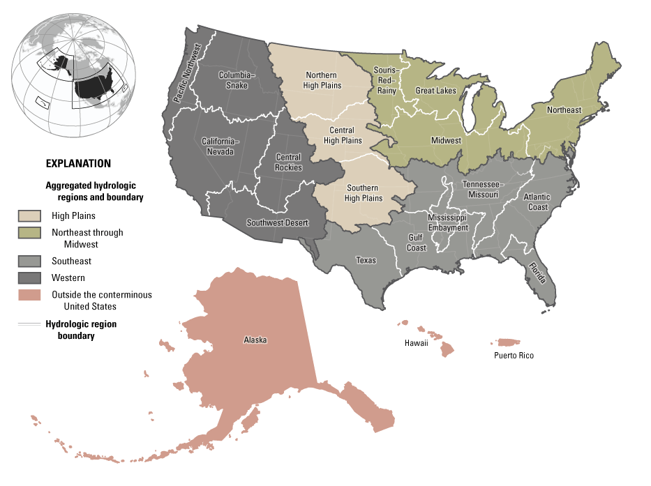
Hydrologic regions and aggregated hydrological regions across the conterminous United States, as well as in Alaska, Hawaii, and Puerto Rico (Van Metre and others, 2020).
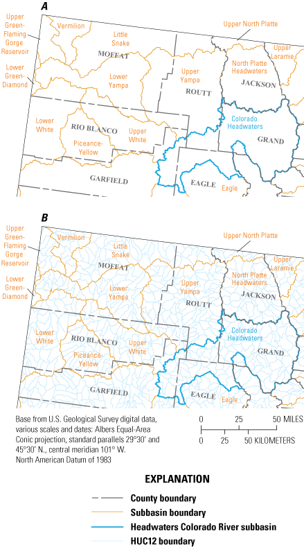
Headwaters Colorado River subbasin overlain with (A) counties and (B) 12-digit hydrologic unit code (HUC12) boundaries.
Terminology and Context
Water-Use Concepts
Water-use terms and concepts used in this chapter are defined in the “Glossary” section and are shown in figure 1. The core concept of water use is the water withdrawal from groundwater or surface water to use for a specific purpose and the return flow back to the local environment. Water is typically moved or conveyed through one or more pipes or canals, or for some larger systems, through tunnels or aqueducts. Water use is typically categorized by type (category) of use, such as public supply, thermoelectric power, irrigation, domestic, or industrial use. Consumptive use is the part of water withdrawn that is evaporated, transpired, incorporated in products or crops, consumed by humans or livestock, or otherwise removed from the immediate water environment. Water that is withdrawn but has not been removed from the local environment is returned to groundwater or surface water as return flow (or effluent), which can occur through various means such as outfall pipes from wastewater treatment or industrial facilities or on-site septic systems. In some areas, often but not always where freshwater resources are scarce, water after treatment, referred to as “reclaimed wastewater” or “reused water,” might be used for potable or non-potable purposes (such as to irrigate crops, lawns, or golf courses) or as cooling water for thermoelectric powerplants. Effluent from wastewater treatment facilities is typically returned to streams and may help sustain minimal flow for ecological purposes and furnish water for downstream withdrawals. Because return flow is available for further instream or offstream use, any chemical or thermal alteration resulting from use has implications for water quality and stream ecology. As water moves through pipes or other conveyances, water volumes can increase through infiltration or inflow, or can decrease through conveyance losses, such as leaks or broken pipes. Open conveyances like canals are subject to losses from evapotranspiration.
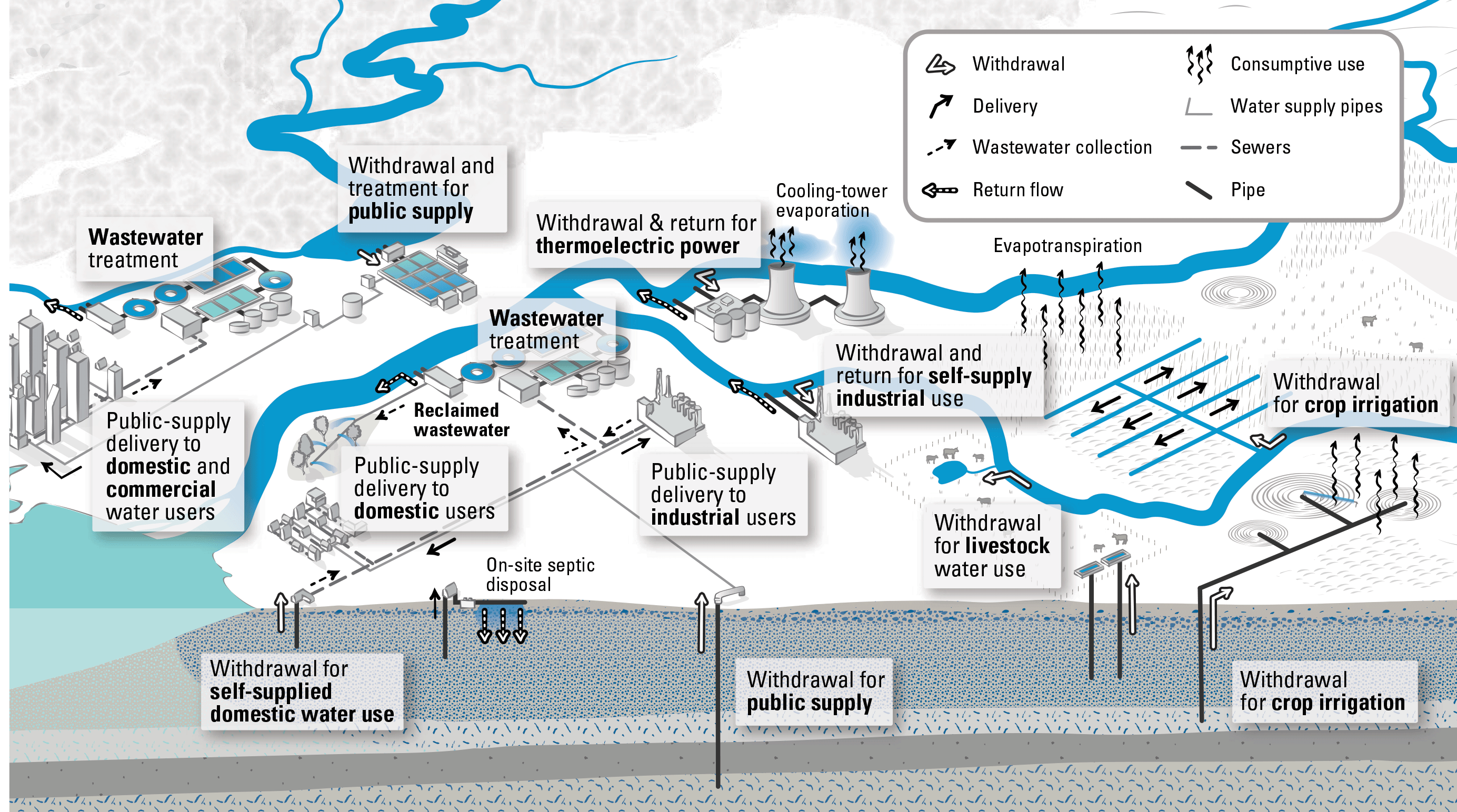
Selected water-use terms and concepts. All possible arrows are not shown in this figure. For example, thermoelectric power facilities may receive water from groundwater, and public supply and industrial facilities that are self-supplied may receive water from groundwater or surface water. Aquaculture and mining water use are not shown. Illustration by Amanda Carr, U.S. Geological Survey.
Water-use terminology is neither static nor universal. The categorization and reporting of water-use information by the USGS water-use program has changed over time. Some organizations or agencies outside the USGS use different terms for water-use concepts or have a different definition for a term used by the USGS. For example, the USGS uses “consumptive use” or “consumption” to mean water that is not readily available for another use locally. Other organizations use the term differently. For example, the Bureau of Reclamation refers to water “consumption” similarly to the USGS except that the term also includes interbasin transfers (Bruce and others, 2018). The South Florida Water Management District issues consumptive water-use permits for water withdrawals. “Water use” and “water withdrawal” can be used interchangeably in many situations, although water use is typically best understood in the context of the category for which it is being used (for example, irrigation or domestic water use) and water withdrawal in the context of removing water from its source (groundwater or surface water).
Public-Supply
This section defines terms and concepts related to public-supply water use by the USGS; terminology associated with self-supply water use is included because it completes the representation of water use for categories such as domestic, industrial, and thermoelectric power. Public-supply water use is defined by the USGS as water withdrawn by public and private water suppliers that furnish water to at least 25 people or have a minimum of 15 connections. The U.S. Environmental Protection Agency uses the same definition for a public water system, which they further classify based on whether or not the populations served are for communities and whether populations are transient or non-transient. Public suppliers provide water for various uses such as domestic, commercial, industrial, thermoelectric power, and public use; the transfers to these water users are referred to as public-supply deliveries. The difference between water withdrawals by public suppliers and deliveries to billed water users is non-revenue water, which includes leakage, meter errors, and public uses of water such as firefighting, street and sewer cleaning, flushing of water lines, irrigation of parks and public lands, and other municipal purposes. Non-revenue water has not historically been accounted for by USGS other than as a calculation of the difference between reported withdrawals and reported or estimated deliveries, resulting in an estimate of “all other uses and losses.” Other terms commonly used outside the USGS to describe public-supply water use are “municipal” or “community” water use.
The phrase, self-supplied water, refers to water used by (1) irrigation, mining, livestock, and aquaculture facilities; and (2) domestic, commercial, and industrial users and thermoelectric-power facilities that is not furnished by a public supplier. For categories that do not receive public-supply water, the term “self-supplied” is often dropped. Water used for crop irrigation is typically self-supplied. Total water use for a given category of use is the sum of water delivered by a public supplier and water that is self-supplied, and for some categories (such as irrigation and thermoelectric) might include reclaimed wastewater.
More information is available for public-supply water use than for self-supplied water use because public suppliers are subject to Federal and State regulations, which typically require some form of data reporting. In contrast, self-supplied water users often have fewer reporting requirements, depending on State or regional regulations. Importantly, although public suppliers generally meter deliveries of water to customers for billing, planning, reporting, and regulatory purposes, metered volumetric data are not always publicly shared. Some self-supplied data are available from States that regulate or require reporting of all types of water withdrawals or withdrawals greater than a designated volumetric threshold or other criteria.
Estimated Water Use by Category
Water-use model estimates are presented for public supply, crop irrigation, and thermoelectric power as 2020 use and as average use during water years 2010–20. Water-use estimates made using previous USGS approaches for calendar year 2015 (or otherwise as noted) are presented for industrial, self-supplied and total domestic, commercial, livestock, mining, and golf course irrigation (sidebar 2). Estimates of water used for energy production, which straddles categories of mining and thermoelectric use, also are presented. The comparability of estimates from the two approaches (previous USGS and modeling) is addressed in interpretive reports (Alzraiee and others, 2024; Harris and others, 2024).
Water Use Estimated Using Modeling Approaches
Because water-use estimates from modeling approaches are associated with places where water is used, not where water is withdrawn (see sidebar 2), these values technically represent estimated water demand. However, to remain consistent with other publications associated with water-use model estimates and with previous USGS approaches to estimating water use (Alzraiee and others, 2024; Dieter and others, 2018a; Haynes and others, 2024), water-use model estimates in this chapter are presented using the terms “water withdrawal” and “water use” interchangeably.
Sidebar 2. Why Change to a Modeling Approach?
Water-use estimates in this chapter were developed using a suite of models to estimate public supply, thermoelectric power, and crop-irrigation water use. These three categories account for about 90 percent of total water withdrawals in the conterminous United States (CONUS; Dieter and others, 2018a).
Models replace previous U.S. Geological Survey (USGS) approaches to estimating water use, which produced annual estimates every 5 years at the State (1950–2015) and county (1985–2015) levels of data aggregation (Dieter and others, 2018a). Previous approaches to estimating water use had numerous shortcomings, including the lack of spatial and temporal granularity and the lack of national uniformity in estimates owing to differences in water-use reporting requirements and data availability between States (Luukkonen and others, 2021).
The hydrologic-based scale of output for model estimates is small watershed (12-digit hydrologic unit code 12 [HUC12]—see sidebar 1), which greatly increases the spatial resolution of water-use estimates and associated data provided by the USGS, from 3,108 counties to 83,074 HUC12s in the CONUS.
Another factor influencing the change to a modeling approach is the need for improved temporal resolution of water-use data. Water-use estimates from models are available at the monthly time step with no gaps during 2000–20 (except for estimates from the thermoelectric power model that begin in 2008). Water-use estimates at the monthly time step enable analysis of seasonal patterns of water use—such as for crop irrigation and public supply outdoor water use—that were previously unattainable.
Other benefits of modeled water-use estimates over previous methods are that they are uniform, documented, and reproducible. Models can be used to evaluate the relative influence of individual components of water supply (streams, aquifers, reservoirs) on the water budget and to assess impacts of changes in land use, climate, and socioeconomic factors on water availability and use. Models also improve understanding of factors that influence water use so that water managers have sufficient information to analyze trends, to plan strategically, and to identify and quantify vulnerability thresholds for adaptive water management.
A caveat of modeling approaches is that water-use estimates are made where water is used, not where water is withdrawn. Native modeling units are public-supply service area for the public-supply model, field for the crop-irrigation model, and powerplant for the thermoelectric power model. For example, water moved through irrigation canals from a reservoir source in Basin A and applied to fields in Basin B is accounted for as a withdrawal in Basin B. Thus, reported locations of some withdrawals are in the incorrect physical basin, which can affect the reliability of water-availability assessments in areas where water is moved across basin boundaries.
For water years 2010–20, average annual estimates of water withdrawals within the CONUS for crop irrigation were 105,497 million gallons per day (Mgal/d), for public supply were 35,440 Mgal/d, and for thermoelectric power from freshwater were 82,656 Mgal/d (12,147, 4,081, and 9,952 million cubic meters per month [Mm3/mo], respectively; tables 1–3, 5–7). Total withdrawals from freshwater for these three categories of use were 223,594 Mgal/d and total withdrawals including saline water for thermoelectric power were 244,817 Mgal/d (26,179 and 28,677 Mm3/mo, respectively; table 4). Monthly values for model estimates are available in data releases on the following subjects: (1) public-supply withdrawals and consumptive use (Luukkonen and others, 2023); (2) crop irrigation consumptive use and withdrawals (Martin and others, 2023; Haynes and others, 2024); and (3) thermoelectric power consumptive use and withdrawals (Galanter and others, 2023).
Table 1.
Model estimates of average annual water withdrawals and consumptive use and the percentage of consumptive use to withdrawals for crop-irrigation water use by aggregated hydrologic regions and total for the conterminous United States (CONUS), water years 2010–20.[Except for percentage (far right column), units are in million gallons per day (top number) and million cubic meters per month (bottom number) for each of the aggregated hydrologic regions. Source data are available in Martin and others, 2023; Haynes and others, 2024]
Table 2.
Model estimates of average annual water withdrawals and consumptive use and the percentage of consumptive use to withdrawals for public-supply water use by aggregated hydrologic regions and total for the conterminous United States (CONUS), water years 2010–20.[Except for percentage (far right column), units are in million gallons per day (top number) and million cubic meters per month (bottom number) for each of the aggregated hydrologic regions. Source data are available in Luukkonen and others, 2023]
Table 3.
Model estimates of average annual water withdrawals and consumptive use and the percentage of consumptive use to withdrawals for thermoelectric water use by aggregated hydrologic regions and total for the conterminous United States (CONUS), water years 2010–20.[Except for percentage (far right column), units are in million gallons per day (top number) and million cubic meters per month (bottom number) for each of the aggregated hydrologic regions. Source data are available in Galanter and others, 2023]
Table 4.
Model estimates of average annual water withdrawals and consumptive use for crop-irrigation, public-supply, and thermoelectric water use by aggregated hydrologic regions and total for the conterminous United States (CONUS), 2010–20.[Units are in million gallons per day (top number) and million cubic meters per month (bottom number) for each of the aggregated hydrologic regions. Source data are available in Galanter and others, 2023; Luukkonen and others, 2023; Martin and others, 2023; Haynes and others, 2024]
Table 5.
Model estimates of average annual water withdrawals and consumptive use and the percentage of consumptive use to withdrawals for crop-irrigation water use by hydrologic region and total for the conterminous United States (CONUS), water years 2010–20.[Except for percentage (far right column), units are in million gallons per day (top number) and million cubic meters per month (bottom number) for each hydrologic region. Source data are available in Martin and others, 2023; Haynes and others, 2024]
Table 6.
Model estimates of average annual water withdrawals and consumptive use and the percentage of consumptive use to withdrawals for public supply water use by hydrologic region and total for the conterminous United States (CONUS),water years 2010–20.[Except for percentage (far right column), units are in million gallons per day (top number) and million cubic meters per month (bottom number) for each hydrologic region. Source data are available in Luukkonen and others, 2023]
Table 7.
Model estimates of average annual water withdrawals and consumptive use and the percentage of consumptive use to withdrawals for thermoelectric-power water use by hydrologic region and total for the conterminous United States (CONUS), water years 2010–20.[Except for percentage (far right column), units are in million gallons per day (top number) and million cubic meters per month (bottom number) for each hydrologic region. Source data are available in Galanter and others, 2023]
Maps show the spatial distribution of water year 2020 model estimates of water withdrawal (fig. 2A–2D). Water withdrawals for the three categories referenced in the previous paragraph of this section vary throughout the CONUS in conjunction with the distribution of population and water resources. Withdrawals for public supply are largest in the Eastern United States (fig. 2A), as well as densely populated urban areas in all States. Although crop-irrigation withdrawals seem to affect a large land mass of the CONUS (fig. 2B), irrigation withdrawals only occur on the part of the HUC12 that is on irrigated land, which in some cases is a small proportion of the HUC12 area. Withdrawals for thermoelectric powerplants are more prevalent and generally larger in the Eastern United States than in the Western United States (fig. 2C). The map of total water withdrawals for the three modeled categories of water use (fig. 2D) essentially shows an integration of areas of withdrawals for public supply and crop irrigation; withdrawals for thermoelectric power seem to be negligible because HUC12s with the largest withdrawals for thermoelectric power are not contiguous and are too small to discern on this page-size map.
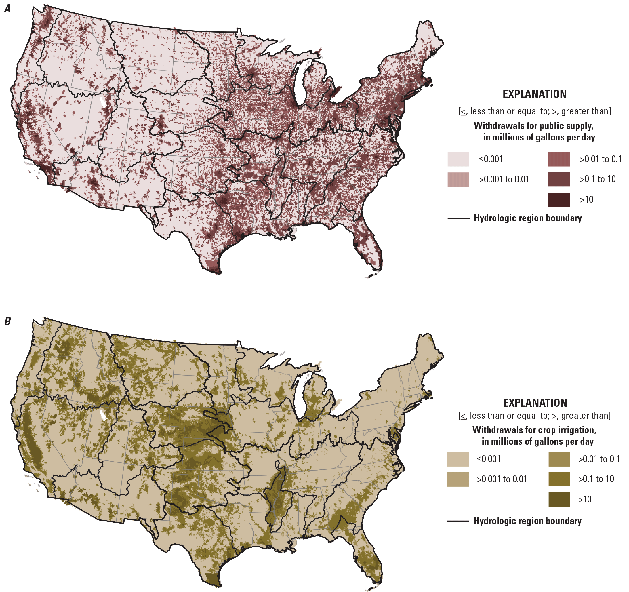
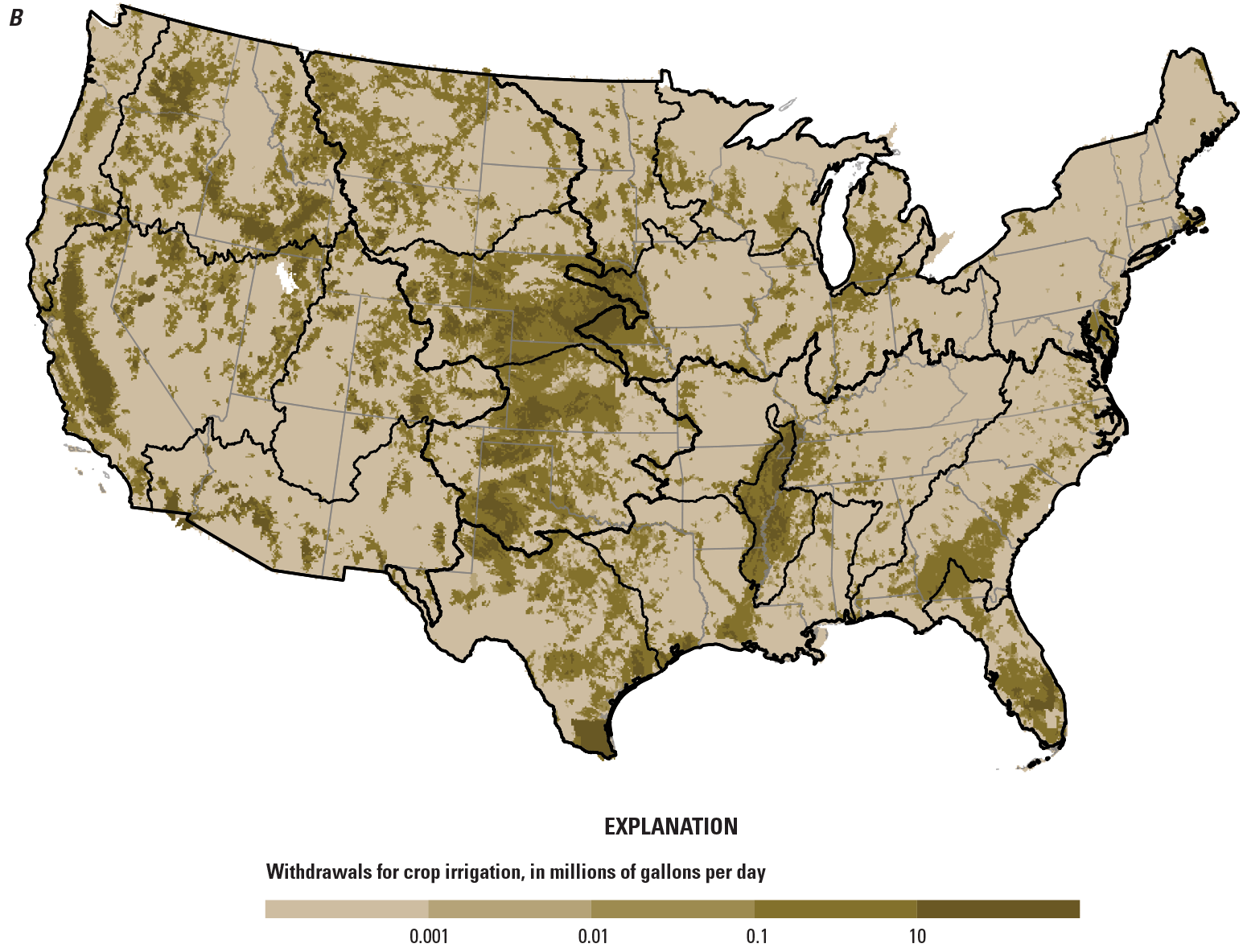
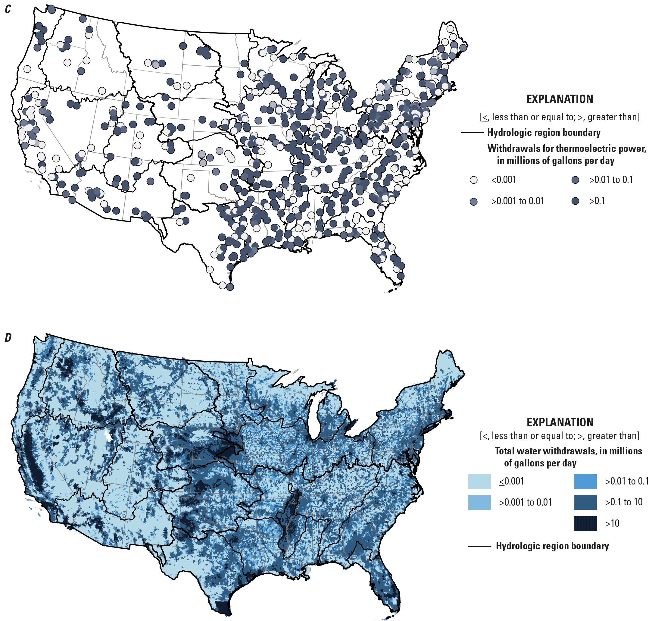
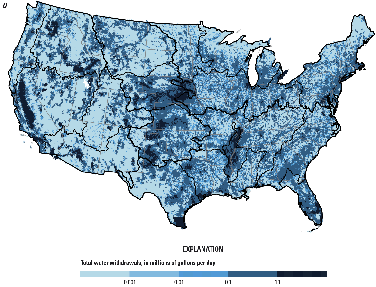
Model estimates showing mean annual water withdrawals for (A) public supply, (B) crop irrigation, (C) thermoelectric-power use, and (D) sum of all three categories, across the conterminous United States (CONUS) by hydrologic regions (indicated by internal black lines) and 12-digit hydrologic unit codes (HUC12s), during water year 2020. Scales are not the same for all maps. Thermoelectric-power water withdrawals include freshwater and saline water. Thermoelectric-power water use map shows symbols for HUC12 centroids because the HUC12s with thermoelectric powerplants are too small to be visible at the CONUS scale. Model estimates for public supply, crop irrigation, and thermoelectric-power water withdrawals are from Luukkonen and others (2023), Haynes and others (2024), and Galanter and others (2023), respectively.
Public-supply, crop-irrigation, and thermoelectric power water-use model results for water year 2020 shown by State, ordered west to east (fig. 3A), reinforce several geographic patterns also evident in the 2015 estimates of water use that were made using previous USGS approaches (Dieter and others, 2018a): crop irrigation is the largest category of use in the western CONUS; (2) thermoelectric power is the largest category of use in the central and eastern CONUS; and (3) public supply accounts for nearly one-half of water withdrawals in some eastern States such as Ohio, New York, and New Jersey. Withdrawals for public supply are largest in states with large populations, such as California, Texas, New York, and Florida.
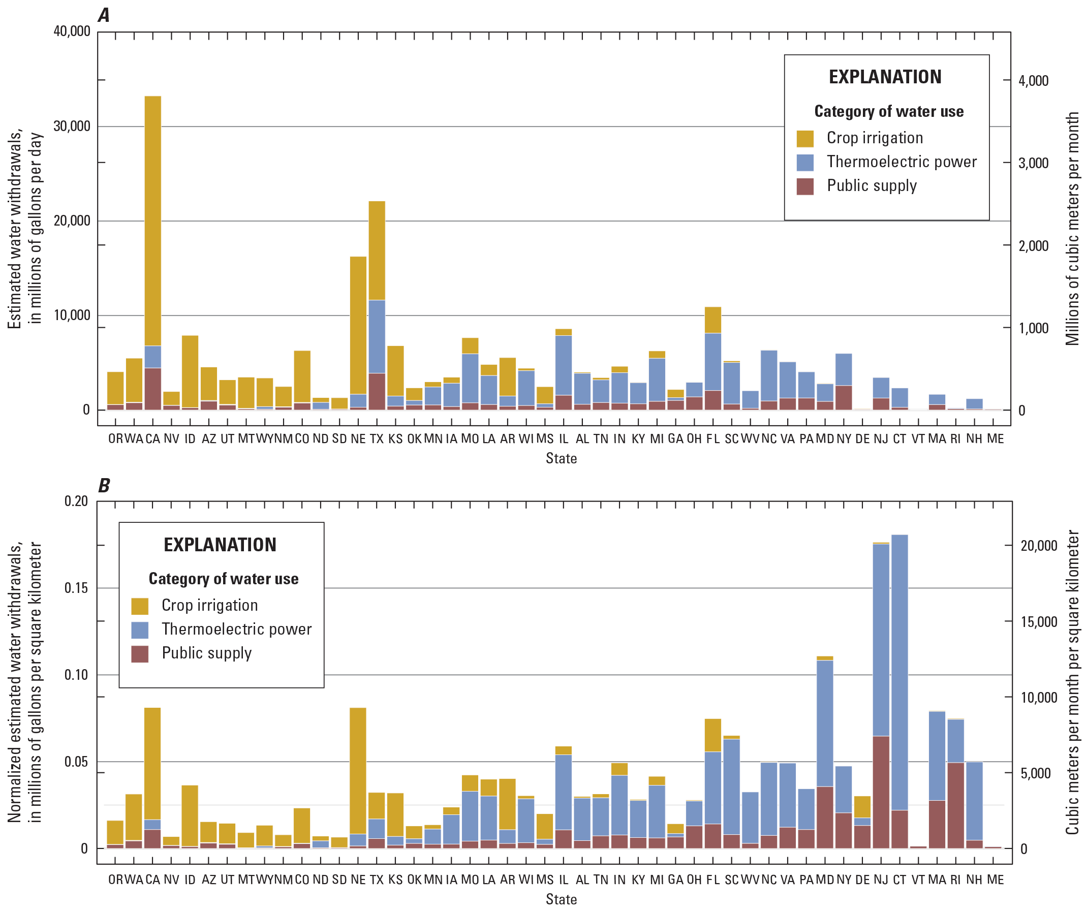
Model estimates of crop-irrigation, thermoelectric-power, and public-supply water withdrawals by State from west to east in the conterminous United States, for water year 2020. Data are shown as (A) not normalized and (B) normalized by area of State. Thermoelectric power water withdrawals include freshwater and saline water. Values for States (which are indicated with 2-digit postal codes) were generated by apportioning 12-digit hydrologic unit code (HUC12) results to States by area. Water withdrawals for some states (Delaware, Vermont, Rhode Island, Maine) are not zero but are too small to appear in the figure. Model estimates for public supply, crop irrigation, and thermoelectric-power water withdrawals are from Galanter and others (2023), Luukkonen and others (2023), and Haynes and others (2024), respectively.
Total estimated withdrawals for crop irrigation, thermoelectric power, and public supply are greater than 20,000 Mgal/d in California and Texas, and are 13,000 in Nebraska, with the largest part of the withdrawal for each of these States being for crop irrigation (fig. 3A). Because consumptive use is a relatively large percentage of the withdrawal for crop-irrigation water use (Martin and others, 2023; Haynes and others, 2024), places where crop-irrigation water use is dominant (western States of Oregon through Kansas in fig. 3A) have large consumptive use losses. Implications for water availability are related to the absolute volume of the withdrawal (immediate removal from the local water resource), the volume of withdrawal lost to consumptive use (sustained removal from the local water resource), and the place of use relative to the withdrawal. The latter point refers to water being moved away from the place of withdrawal in constructed conveyances; if the movement crosses a hydrologic boundary, it is referred to as an interbasin transfer (see section, “Interbasin Transfers”).
Area-normalized water-withdrawal estimates (dividing withdrawals by total area of each State; fig. 3B) enables comparisons of the water-withdrawal intensity among States. Water-withdrawal intensity is particularly large for eastern states because their smaller areas amplify the normalized estimates. Connecticut, New Jersey, and Maryland are the largest States in terms of total normalized withdrawals or water-use intensity, whereas California and Texas, with large total withdrawals (fig. 3A), are lower in water-use intensity (fig. 3B).
Modeled estimates of water use also provide insight into year-to-year variability. Annual total water use for the CONUS for water years 2010–20 for thermoelectric fresh and saline, public supply, and crop irrigation water use is shown in figure 4. During this period, public-supply withdrawals are relatively constant, ranging from 34,778 in 2010 to 36,195 Mgal/d in 2018 (4,004 to 4,167 Mm3/mo, respectively). The lowest and highest withdrawals for crop-irrigation water use occurred in 2019 and 2012, respectively (90,207 and 124,637 Mgal/d; 10,392 and 14,359 Mm3/mo), although withdrawals between these years show no pattern. In contrast, model estimates show a steady 40 percent decrease in withdrawals from freshwater for thermoelectric power, from 102,978 Mgal/d in 2010 to 61,399 Mgal/d in 2020 (11,871 to 7,099 Mm3/mo). Different input datasets and methods might contribute to decreased water-use estimates for thermoelectric power, although at least some of the decreases between 2015 and 2020 can be attributed to changes in plant types and plant closures (Harris and others, 2024; Harris and Diehl, 2019). The decrease in withdrawals for thermoelectric power for water years 2010–20 is the primary factor controlling the decrease in total withdrawals for these three categories over the given time period.
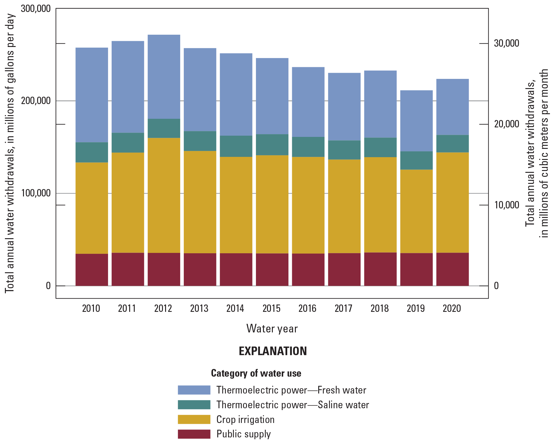
Model estimates of total annual water withdrawals for thermoelectric power (saline and freshwater), crop irrigation, and public supply for the conterminous United States, water years 2010–20. Model estimates for thermoelectric-power, crop irrigation, and public supply water withdrawals are from Galanter and others (2023), Luukkonen and others (2023), and Haynes and others (2024), respectively.
Public-Supply Water Withdrawals, Consumptive Use, and Per-Capita Use
Model estimates for water withdrawals1 and consumptive use for public supply for the CONUS in water year 2020 were 35,943 and 4,157 Mgal/d, respectively (fig. 5; 4,138 and 479 Mm3/mo). These values are similar to the modeled average withdrawals and consumptive use for public supply during 2010–20 of 35,440 and 4,219 Mgal/d (tables 2 and 6; 4,081 and 486 Mm3/mo). The ratio of public-supply consumptive use to withdrawals varies by hydrologic region, from 0.08 in the Gulf Coast, Atlantic Coast, and Great Lakes to 0.23 in the Southwest Desert, with the overall average across the CONUS of 0.12 (table 6). Most water used for public supply is returned to the local environment. In some areas, large volumes of public-supply water are neither lost to consumptive use nor returned to the local environment of the withdrawal because the use of that water is in a different watershed than the withdrawal (see section, “Interbasin Transfers”). During 2010–20, model estimates for public-supply water withdrawals and consumptive use produced values that varied by 4 and 20 percent, respectively (fig. 5; Luukkonen and others, 2023).
The 2015 estimates of total water withdrawals for public supply included 270 million gallons per day of desalinated seawater or treated brackish groundwater from seven States in the conterminous United States plus the U.S. Virgin Islands, representing less than 1 percent of total public-supply withdrawals (Dieter and others, 2018a). Modeled estimates of withdrawals used for public supply do not distinguish saline or brackish water from fresh water (Luukkonen and others, 2023).
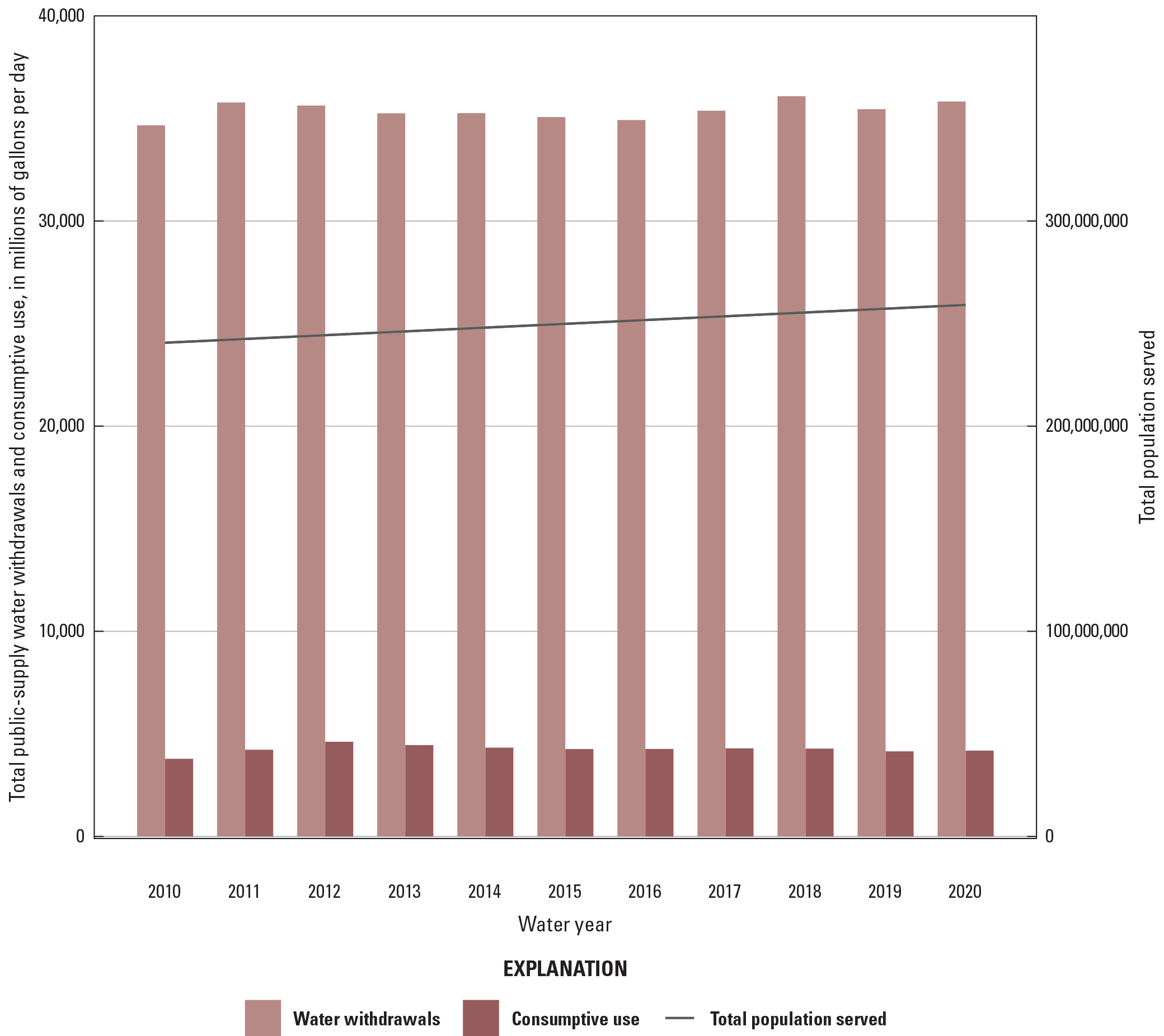
Model estimates of public-supply water withdrawals, consumptive use, and total population served for the conterminous United States, water years 2010–20. Model estimates for public supply water withdrawals, consumptive use, and population served are from Luukkonen and others (2023).
Populations served by public supply increased consistently on an annual basis by a total of 8 percent during 2010–20 (fig. 5). We hypothesize that overall public-supply withdrawals are relatively unchanged over this time period while populations served are increasing because of increased water-efficiency measures such as improved metering, more effective water-use auditing procedures and rate structuring, efforts to control leaks and water losses, and a better understanding of customer water use (U.S. Environmental Protection Agency, 2016). Model estimates of public-supply withdrawals are strongly related to population served for estimates aggregated to hydrologic regions (coefficient of determination [R2] = 0.96; fig. 6). This relation is expected given that on a national basis, about 60 percent of total water withdrawals for public supply are delivered to domestic users (Dieter and others, 2018a). Most of the remaining (non-domestic) water withdrawals for public supply are delivered to other types of water users such as industrial, thermoelectric, or commercial users.
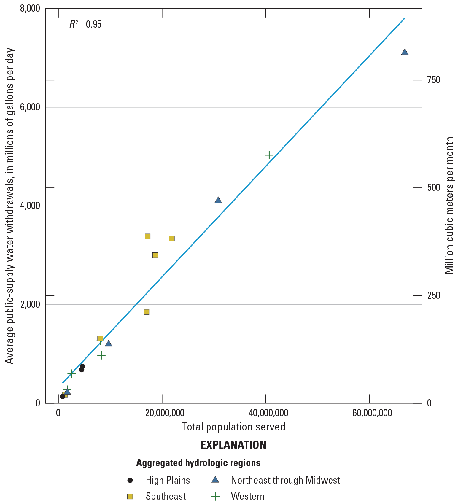
Model estimates comparing public-supply water withdrawals with population served for hydrologic regions of the conterminous United States, averaged over 2010–20. Each symbol represents a hydrologic region. Calendar years, rather than water years, are presented because information on population served is not available for water years. R2, coefficient of determination. Model estimates for public supply water withdrawals and population served are from Luukkonen and others (2023).
Spatial representations of public-supply water withdrawals, consumptive use, and per-capita use (calculated as total withdrawal for public supply divided by population served) vary across the CONUS (fig. 7). Almost three-quarters of total withdrawals in the CONUS occur in the Southeast and Northeast through Midwest aggregated hydrologic regions (table 2; fig. 7A, 7B), despite the California–Nevada hydrologic region (one of the Western aggregated hydrologic regions) accounting for 14 percent of total public-supply water withdrawals in the CONUS (table 6). Although withdrawals are greater in the Eastern United States, consumptive use is a slightly greater percentage of public-supply water withdrawals in the Western and High Plains aggregated hydrologic regions compared to the Southeast and Northeast through Midwest aggregated hydrologic regions (table 2; fig. 7D). Conversely, average per-capita use is 21 percent greater in the two western aggregated hydrologic regions than in the two eastern aggregated hydrologic regions (fig. 7F). Population served (and by extension, water withdrawals for public supply) is inversely related to per-capita water use because water efficiency in large cities with greater housing density is often greater than in smaller cities (Alzraiee and others, 2024; Mahjabin and others, 2018; Chinnasamy and others, 2021).
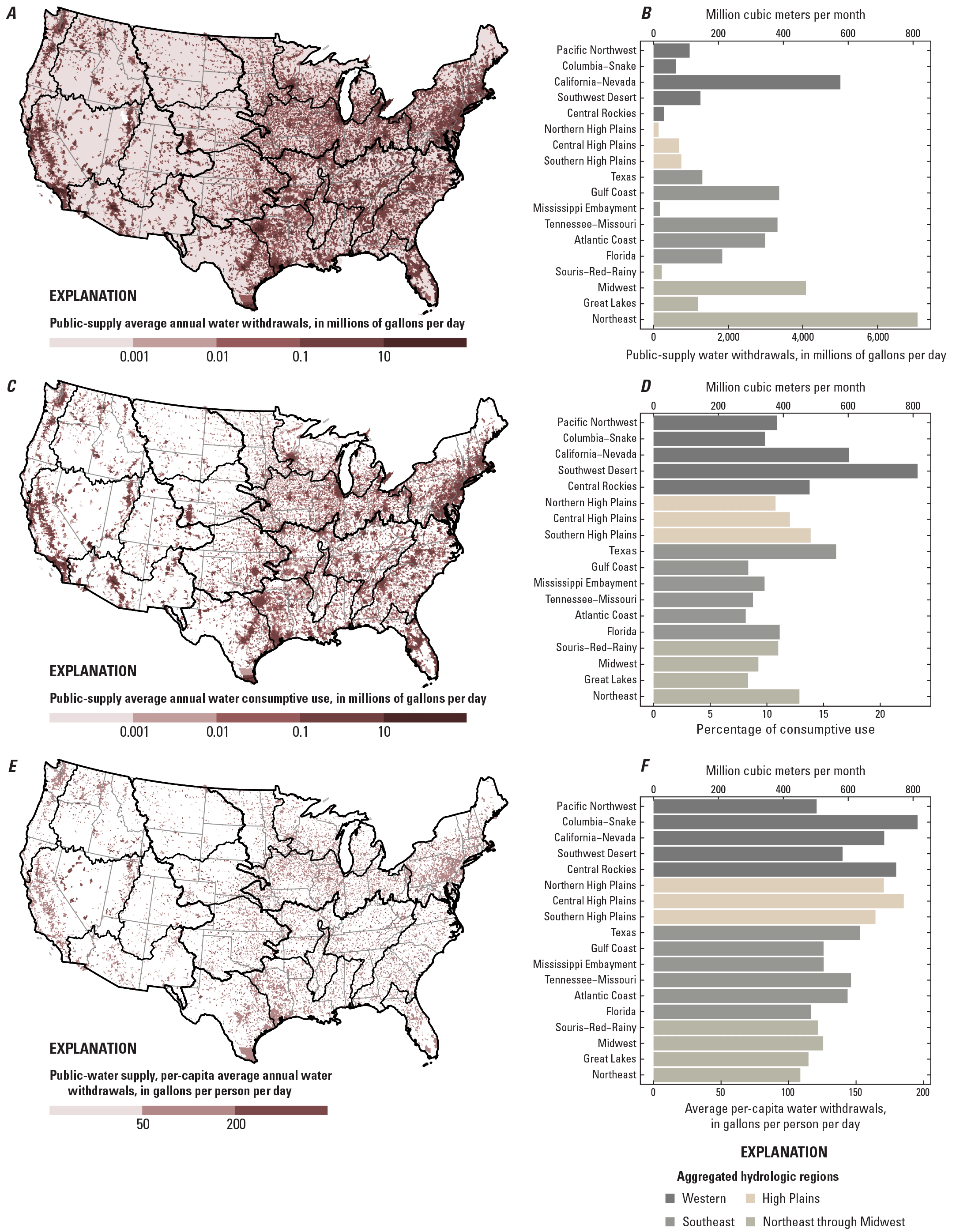
Maps—compiled from 12-digit hydrologic unit code data—and bar graphs—organized by hydrologic region and aggregated hydrologic regions—showing model estimates of public-supply (A, B) average annual water withdrawals; (C) average annual water consumptive use; (D) average annual water consumptive use as a percentage of average annual withdrawal; and (E, F) average annual per-capita water withdrawals, 2010–20. Data for figure 7A–7D is by water year. Data for figure 7E–7F is for calendar year because annual per-capita estimates were made on the basis of calendar year and are not available for months or water years. Black lines in figure 7A, 7C, and 7E indicate hydrologic region boundaries. Model estimates for all elements of this figure are from Luukkonen and others (2023).
Implications of these patterns for water availability are apparent when considering withdrawals and the relative volumes of public-supply water removed from the local environment as consumptive use. Consumptive-use percentages are larger in arid parts of the country (such as the Southwest Desert, California–Nevada, and Texas hydrologic regions) compared to the wetter Eastern United States (table 6; fig. 7D) primarily because more public-supply water is used for landscape irrigation in arid areas, a large part of which is evapotranspired (Alzraiee and others, 2024; Chinnasamy and others, 2021).
Precipitation is another factor that influences public-supply water use overall across the CONUS as well as within hydrologic regions (fig. 8). Across the CONUS, annual average per-capita water withdrawals decrease as precipitation increases, with 57 percent of the variation (R2 = 0.57) in per-capita withdrawals explained by precipitation (fig. 8B). Less public-supply water is used during wet periods to satisfy demands for outdoor water use (Worland and others, 2018; Chinnasamy and others, 2021; Alzraiee and others, 2024). In contrast to other hydrologic regions, the Pacific Northwest, Columbia–Snake, and Northeast hydrologic regions have weak positive relations (R2 values are equal to or less than 0.12) indicating that the relation between per-capita use and precipitation is spurious (fig. 8A). Two of these regions—the Northeast and Pacific Northwest regions—have relatively low average per-capita use rates and large annual precipitation compared to other regions, indicating less outdoor water use and consequently, less of a dependence on precipitation.
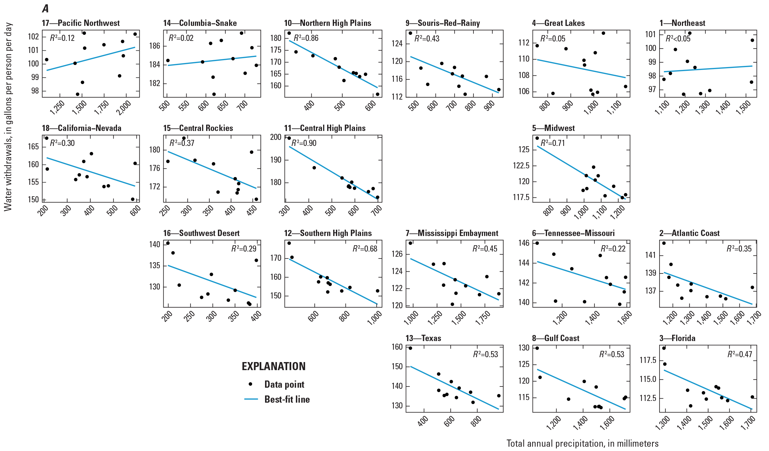
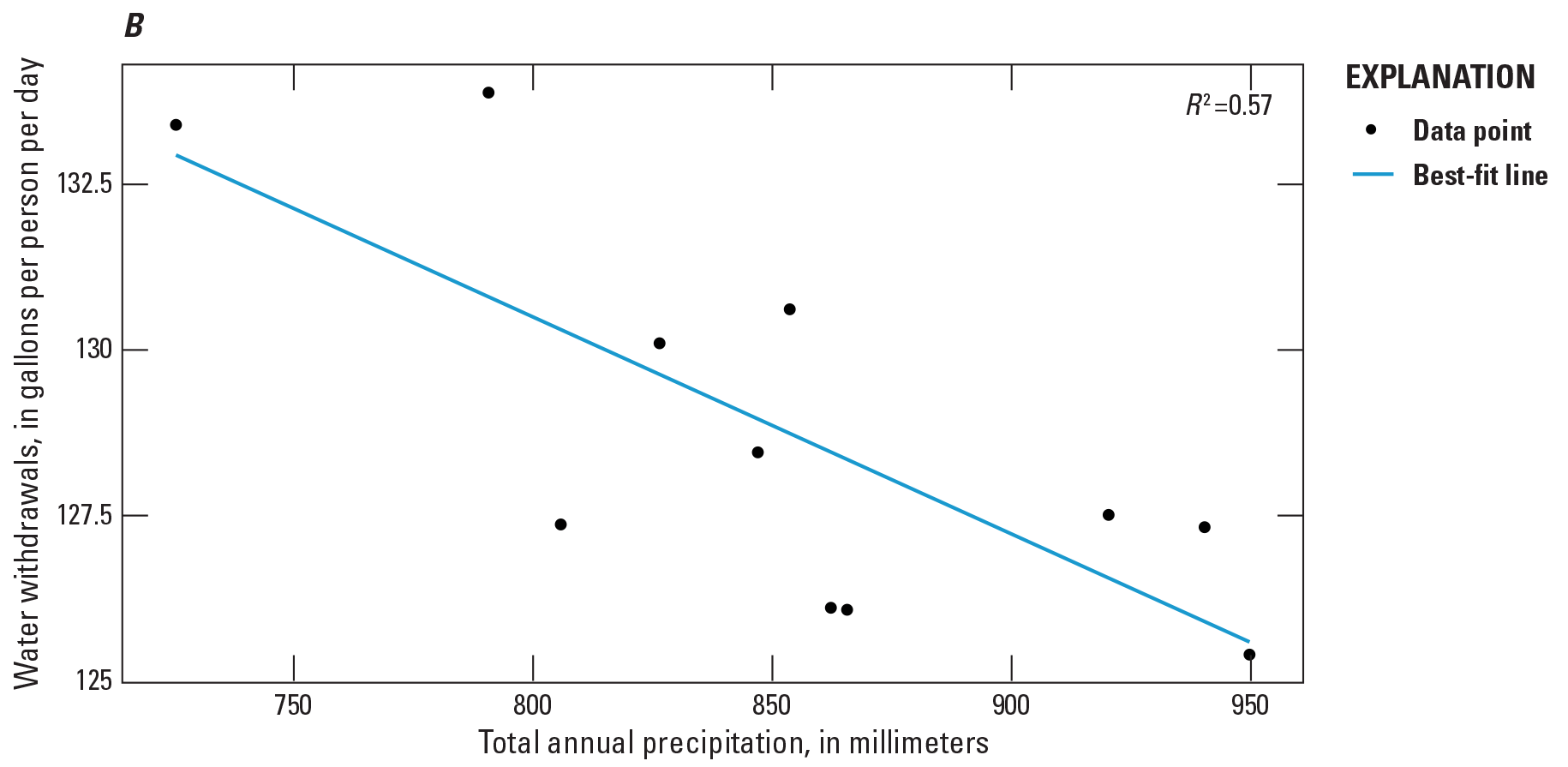
Model estimates of annual average public-supply per-capita water withdrawals compared to precipitation (A) by hydrologic region and (B) overall for the conterminous United States, 2010–20. Scales are different for each figure. R2, coefficient of determination. Model estimates for public-supply per-capita water withdrawals are from Luukkonen and others (2023). Precipitation data are from Foks and others (2024).
Seasonal as well as spatial variations are important characteristics of water-use data used for water-availability studies. A base level of water deliveries from public suppliers to domestic users for indoor uses like cooking, washing, and flushing toilets is relatively insensitive to seasonal fluctuations. Additional water demand for seasonal (outdoor) water uses can add substantially to the base-level demand. Seasonal variations in public-supply water use reflect the same influences in outdoor water demand that were discussed previously in the context of consumptive use as a percentage of total withdrawals for public supply. Because outdoor water demand varies across the CONUS, seasonal fluctuations in public-supply water use likewise vary across hydrologic regions and aggregated hydrologic regions (fig. 9), with the Western and High Plains aggregated hydrologic regions showing much greater ranges in public-supply withdrawals between months of the year compared to the Southeast and Northeast through Midwest aggregated hydrologic regions.
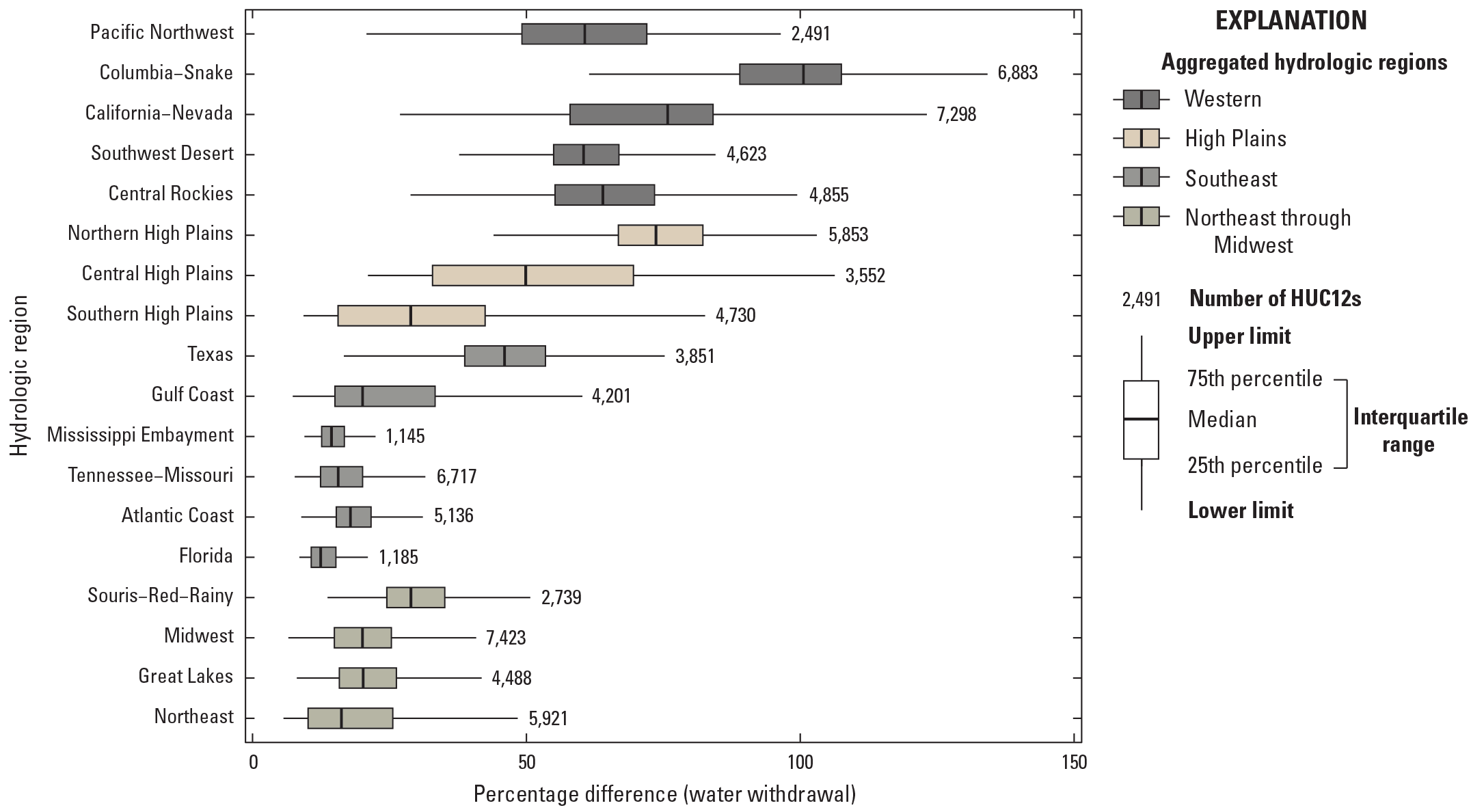
Percentage difference between minimum and maximum monthly model estimates of average public-supply water withdrawals for 12-digit hydrologic unit codes (HUC12s) grouped by hydrologic regions and aggregated hydrologic regions, water years 2010–20. Wider bars indicate greater seasonal fluctuation in water use. Model estimates for public-supply water withdrawals are from Luukkonen and others (2023).
Although regions or areas with large intra-annual fluctuations in public-supply water withdrawals have greater amounts of outdoor water use for at least some months of the year (Dieter and others, 2018a; Chinnasamy and others 2021; Alzraiee and others, 2024), other factors also likely contribute to seasonal differences in public-supply withdrawals. For example, cold-season losses from public-supply distribution lines attributable to burst or leaking pipes from freeze-thaw cycles can increase winter public-supply water withdrawals in northern areas of the country (Alzraiee and others, 2024). Seasonal tourism or migrations for work affect intra-annual variations in local public-supply water demand. Some northern or mountainous parts of the country that have sufficient snow attract skiers or snowmobilers who use public-supply water in winter, if within a service area, for second homes, condominiums, hotels, and restaurants (Medalie and Horn, 2010).
The pattern of seasonal public-supply consumptive use is similar to that for public-supply withdrawals, with some notable differences (figs. 9 and 10). Rather than following the prominent east-west distinction of percentage differences in the range of monthly public-supply withdrawals in figure 9, consumptive use estimates in the Northeast through Midwest aggregated hydrologic regions (Souris–Red–Rainy, Midwest, Great Lakes, and Northeast hydrologic regions) are patterned more like western than eastern areas (fig. 10). The Northeast through Midwest aggregated hydrologic regions, like the Western and High Plains aggregated hydrologic regions, have large monthly fluctuations in evapotranspiration, which is a substantial factor in estimates of consumptive use for public supply but not in withdrawals. Conversely, the Southeast aggregated hydrologic regions (Texas, Gulf Coast, Mississippi embayment, Tennessee–Missouri, Atlantic Coast, and Florida hydrologic regions) have smaller monthly ranges in consumptive-use estimates because seasonal evapotranspiration changes are relatively small (chap. B, Gorski and others, 2025). The interquartile range of consumptive use for Texas is particularly small because monthly estimates of consumptive-use are relatively stable among HUC12s in that region.
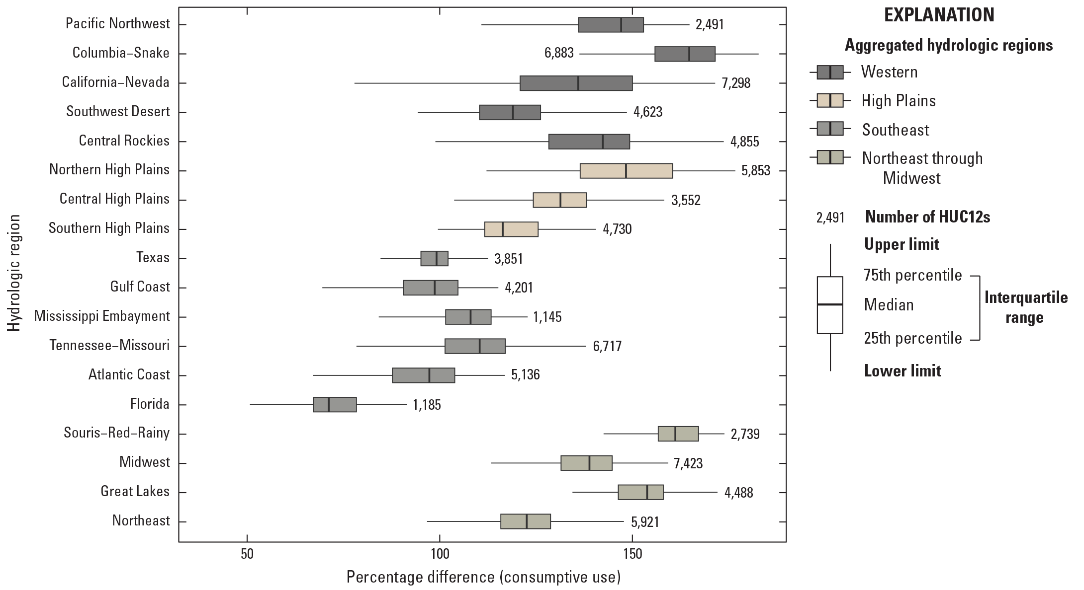
Percentage difference between minimum and maximum monthly model estimates of average public-supply consumptive use for 12-digit hydrologic unit codes (HUC12s) grouped by hydrologic regions and aggregated hydrologic regions, water years 2010–20. Model estimates for public-supply consumptive use are from Luukkonen and others (2023).
Crop-Irrigation Withdrawals and Consumptive Use
Crop irrigation accounted for the largest withdrawals of freshwater across the CONUS during water years 2010–20 (fig. 4). Average water withdrawals and consumptive use for crop irrigation during 2010–20 were 105,497 and 75,698 Mgal/d (12,147 and 8,716 Mm3/mo), respectively (table 1). Model estimates for water withdrawals and consumptive use for crop irrigation for the CONUS in water year 2020 were 108,723 and 78,400 Mgal/d (12,526 and 9,027 Mm3/mo), respectively. Model estimates for crop-irrigation withdrawals and consumptive use have a nearly identical pattern (fig. 11) because irrigation withdrawals are calculated from modeled irrigation consumptive use and irrigation efficiency (Haynes and others, 2024). Modeled crop-irrigation consumptive use for hydrologic regions varied from 59 to 84 percent of the estimated crop-irrigation withdrawals, with largest percents in the Northeast through Midwest aggregated hydrologic regions and smallest percents in the Western aggregated hydrologic regions and a national average of 72 percent (tables 1 and 5; Martin and others, 2023; Haynes and others, 2024).
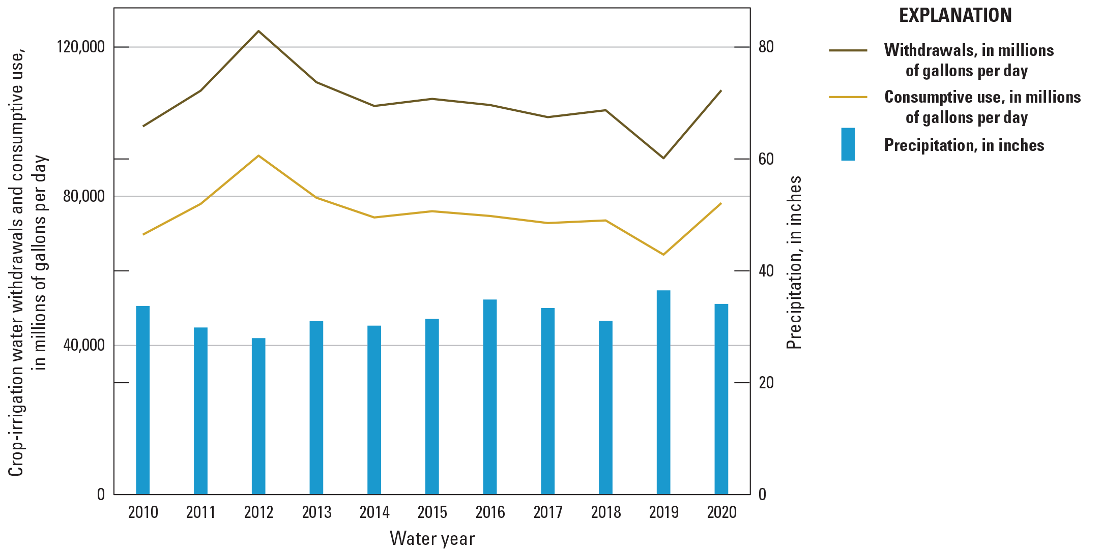
Time series graph of annual total precipitation and model estimates of crop-irrigation water withdrawals and consumptive use in the conterminous United States, water years 2010–20. Model estimates for crop-irrigation water withdrawals and consumptive use are from Haynes and others (2024). Data for total precipitation are from the National Oceanic and Atmospheric Administration (2023).
In addition to water applied by an irrigation system to grow crops and pastures, model estimates of crop-irrigation water withdrawals include water losses from irrigation systems and conveyance losses (Haynes and others, 2024). Estimates of irrigation water use made using previous USGS approaches also included pre-growing season applications, frost protection, chemical application, weed control, field preparation, crop cooling, harvesting, dust suppression, and leaching salts from the root zone (Dieter and others, 2018a). In the CONUS in 2017, crops with the largest number of irrigated acres, in descending order, were corn for grain, soybeans, hay and alfalfa, orchards, and cotton (U.S. Department of Agriculture, 2019).
Crop-irrigation water use is largely a function of climate variables such as precipitation and evaporative demand (Nie and others, 2021). Crop-irrigation withdrawals and consumptive use are generally inversely related to precipitation (fig. 11; the correlation coefficient for precipitation and crop-irrigation consumptive use is −0.77). A severe multi-year drought across much of the United States during 1999–15 was most intense in 2012 (Hoerling and others, 2014; McCabe and others, 2023). Estimates of annual crop-irrigation withdrawals and consumptive use during 2012 increased by more than 28 and 43 percent, respectively, compared to the wettest year (2019) and crop-irrigation withdrawals were 13 percent greater than the next driest year (2011) during 2010–20 (fig. 11).
Crop-irrigation water withdrawals during water year 2012 compared to the average of water years 2010−20 were not uniform across the CONUS (fig. 12). Compared to average May crop-irrigation withdrawals, water year 2010−20 withdrawals in May 2012 were about 14 and 9 times higher in the Mississippi embayment and Central High Plains hydrologic regions, respectively (fig. 12). In contrast, the Pacific Northwest, Columbia–Snake, Texas, and Florida hydrologic regions had smaller crop-irrigation withdrawals in May 2012 compared to water years 2010−20 (fig. 12). Other factors besides climate (such as irrigation management, irrigation infrastructure, and crop type) also highly influence crop-irrigation water withdrawals (Ketchum and others, 2023).
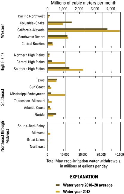
Comparison of total May crop-irrigation water withdrawals across hydrologic regions and aggregated hydrologic regions in the conterminous United States for water years 2010–20 and water year 2012. Model estimates for crop-irrigation water withdrawals are from Haynes and others (2024).
Satellite data show that for areas that grow crops, irrigated-land footprints vary from year to year, with an overall increasing trend in total area of irrigated land in the United States since 1997 (Xie and others, 2021). During drought, even with less irrigated land, crop needs for irrigation are greater than during normal or wet years and more water is lost as consumptive use to evapotranspiration. The percentage of crop-irrigation consumptive use to withdrawals in 2012 was 73, compared to the lowest percentage of 70.4 percent in 2010 (Martin and others, 2023; Haynes and others, 2024).
Monthly estimates of crop-irrigation water use at the HUC12 scale during 2010–20 show that irrigation water is used most heavily in the Central Valley of California, the Snake and Yakima River Basins in Idaho and Washington, and southern Florida and Texas, as well as the Central High Plains, Southern High Plains, and Mississippi Embayment hydrologic regions, and that most crop-irrigation use occurs from May to October (fig. 13). Crop-irrigation withdrawals generally increase northward as temperatures warm and decrease again in late autumn after crops are harvested. Some parts of the country have a climate that is conducive for growing crops in all seasons. For example, grains, hay, cotton, tomatoes and other row crops, citrus, nuts (almonds, walnuts, and pistachios), and grapes are grown year-round in Fresno County in the Central Valley of California (Fresno County Department of Agriculture, 2010). Because crop irrigation accounts for the largest volume of water use across the CONUS, and withdrawals from some small watersheds (HUC12 scale) in some parts of the country during summer are very large (more than 10 Mgal/d; fig. 13), the absolute and relative volumes of crop-irrigation withdrawals and consumptive use are important to water-availability assessments at small and large spatial scales.
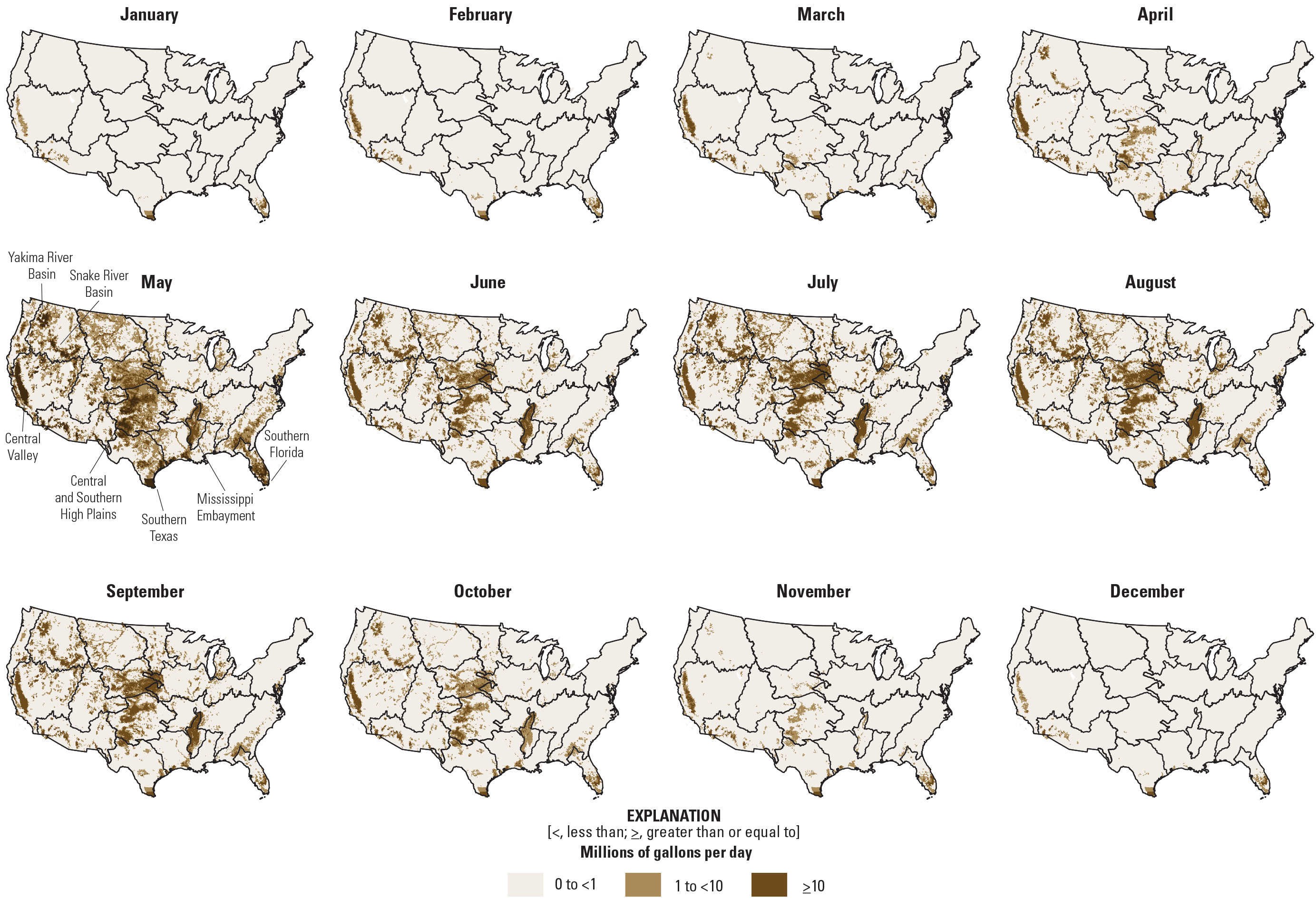
Model estimates of crop-irrigation water withdrawals by month by 12-digit hydrologic unit codes (HUC12s) for the conterminous United States, averaged for water years 2010–20. Black lines indicate hydrologic region boundaries. Model estimates for crop-irrigation water withdrawals are from Haynes and others (2024).
The largest estimated water use for crop irrigation for the CONUS occurred in July. Median modeled estimates for July crop-irrigation withdrawals, summed to hydrologic regions during water years 2010–20, ranged from 650 Mgal/d in the Northeast hydrologic region to 61,328 Mgal/d in the California–Nevada hydrologic region (fig. 14A; 75 to 7,065 Mm3/mo). Estimates of crop-irrigation consumptive use are similarly framed by a low estimate of 527 Mgal/d in the Northeast and a high of 41,212 Mgal/d in the California–Nevada hydrologic region (fig. 14A; 61 to 4,748 Mm3/mo).
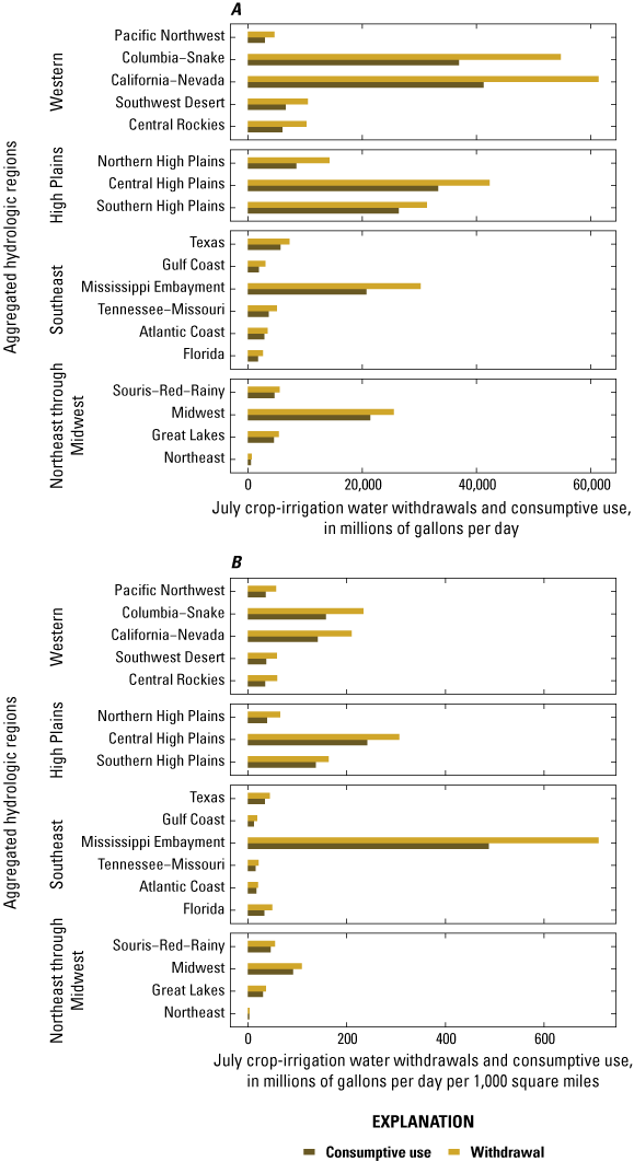
Model estimates of crop-irrigation water withdrawals and consumptive use with median July values for 12-digit hydrologic unit codes (HUC12s), summed by hydrologic regions, showing (A) total values and (B) values normalized by the area of each hydrologic region in the conterminous United States, for water years 2010–20. Model estimates for crop-irrigation water withdrawals and consumptive use are from Haynes and others (2024).
Normalizing by area and expressing as a depth (volume divided by area) provides an indication of the intensity of crop-irrigation withdrawals and consumptive use within each region, which influences regional water availability. More intense withdrawals and consumptive use place a greater degree of hydrologic stress on the region. The Northeast hydrologic region has the least intense crop-irrigation withdrawal, 0.000016 feet per year (ft/yr), and the Mississippi Embayment hydrologic region has the most intense average July crop-irrigation withdrawal, 0.0034 ft/yr—more than double the average July withdrawal of 0.0015 ft/yr for the next most intense region, the Central High Plains (0.005, 1.04, and 0.46 millimeters per year, respectively; fig. 14B). Normalized consumptive use estimates for crop irrigation follow the same pattern as normalized withdrawals.
Why are normalized withdrawals and consumptive use so much higher in the Mississippi Embayment than other parts of the country? The Mississippi Embayment hydrologic region, substantially overlapping with the Mississippi Alluvial Plain aquifer system, is one of the most productive agricultural regions in the Nation and depends largely on groundwater for irrigating rice, a water intensive crop, and other crops. In the Mississippi Embayment hydrologic region, which covers a relatively small area (43,000 square miles [mi2]) compared to most of the other hydrologic regions, cultivated cropland accounts for about 45 percent of the land area with 7 percent used for rice production (Karaba and others, 2007). The combination of small area and large withdrawals for crop-irrigation needs can explain the amplified intensity of crop-irrigation withdrawals from the Mississippi Embayment hydrologic region and concomitant water stress (chap. F, Stets and others, 2025b).
Thermoelectric Power Withdrawals and Consumptive Use
Thermoelectric-power water use is characterized by large withdrawals and relatively low consumptive use (Diehl and Harris, 2014; Harris and Diehl, 2019). Model estimates for withdrawals within the CONUS for thermoelectric power in water year 2020 were 61,399 Mgal/d from fresh water and 19,033 Mgal/d from saline water, totaling 80,432 Mgal/d (7,099, 2,194, and 9,293 Mm3/mo, respectively). Average withdrawals from fresh water for thermoelectric power during water years 2010–20 were 82,656 Mgal/d and from saline water were 21,224 Mgal/d (9,952 and 2,497 Mm3/mo, respectively). Different types of cooling systems use vastly different amounts of water. Consumptive use for thermoelectric power, overwhelmingly fresh water, was 2,382 Mgal/d in 2020 and 2,904 Mgal/d averaged over water years 2010–20 for the CONUS, or 4 percent of thermoelectric freshwater withdrawals.
Two broad types of cooling systems are once-through and recirculating. Once-through cooling systems withdraw large volumes of water that circulate through powerplant condensers to condense the steam used to generate electricity. Heated water is discharged back to the source; a relatively small amount of that water is consumed through evaporation. Recirculating cooling systems reuse water within the cooling system multiple times and consequently withdraw less from a water source but consume, through evaporation, a larger percentage of the water withdrawn as compared with once-through cooling systems. Consumptive-use rates in plants with recirculating systems can be as much as or greater than 70 percent of withdrawals (Harris and Diehl, 2019). During 2010–20, an overall shift occurred in powerplant infrastructure from once-through cooling systems towards recirculating cooling systems and, as a consequence, withdrawals for thermoelectric power have decreased while the relative amount of consumptive use to withdrawals has increased (Harris and others, 2024).
The type of cooling system for thermoelectric power is directly relevant to understanding water availability. Although withdrawals from thermoelectric powerplants with once-through cooling systems can dominate total water withdrawals across hydrologic regions or States (Dieter and others, 2018a), withdrawals occur at point locations and are much more acutely manifest in the context of water availability at smaller scales such as HUC12. Other than those that use municipal water or reclaimed wastewater, most thermoelectric powerplants are purposefully built near a source of water that can be used for cooling. Unlike with public-supply or crop-irrigation water use, the need to account for interbasin transfers of water for thermoelectric-power water use is negligible. Because the place of use is close to the withdrawal, consumptive use for thermoelectric power also occurs at the location of the plant. This means that locations with plants with recirculating towers, which consume relatively larger volumes of water than other types of cooling systems, have less water available for other uses than locations without these types of plants.
Although included in the USGS thermoelectric power water-use model, discussions of thermoelectric-power water use in this chapter do not include water from public-supply (referred to as “municipal” water sources in Galanter and others, 2023) or reclaimed wastewater. Public-supply and reclaimed wastewater sources contributed water for cooling to about 24 percent of powerplants that were modeled, which generated about 12 percent of total electricity; however, powerplants with these sources of water accounted for a small fraction of thermoelectric withdrawals (0.4 percent) and consumptive use (9 percent) of totals within the CONUS (Galanter and others, 2023). Although these water sources may be important locally, they do not affect our large-scale assessments of water use at the regional and CONUS scale.
Model 2020 estimates of thermoelectric power water withdrawals and consumptive use and their relative percentages—which provide inherent information about the type of cooling system—are shown in figure 15. Figure 16 shows summaries for water years 2010–20. Freshwater withdrawals and the number of powerplants are greatest in the Eastern United States (figs. 15A and 16C), where surface-water availability is greater and once-through cooling systems, characterized by large withdrawal and small consumptive use rates, are more common than in the West. The western CONUS is dominated by thermoelectric powerplants that recirculate cooling water; have relatively large consumptive use rates; and are likely to use groundwater, municipal water, reclaimed wastewater, or a combination thereof (Galanter and others, 2023). These regional patterns are shown by the higher ratio of consumptive use to withdrawals and fewer thermoelectric power plants in the West compared to the East (fig. 15B, 15C).
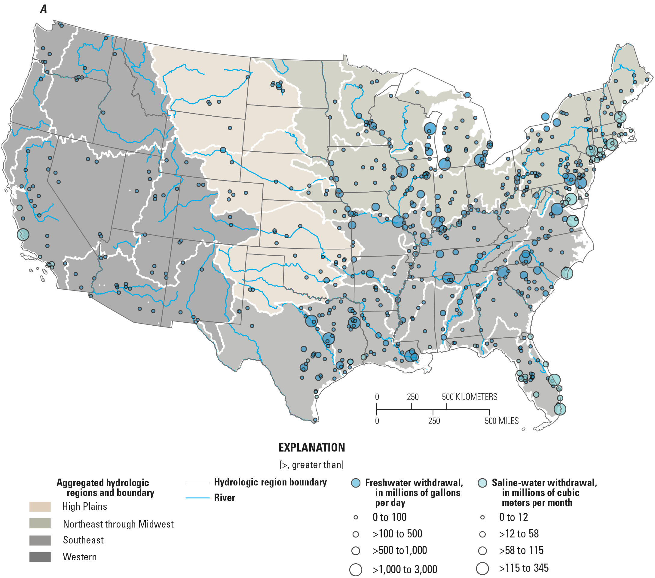
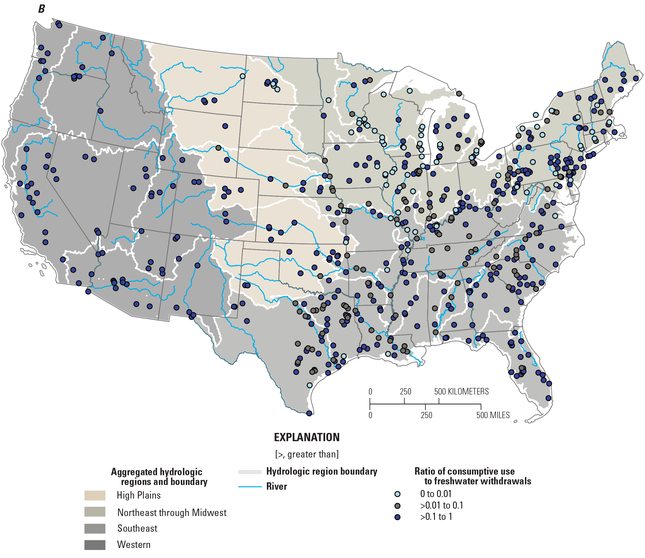
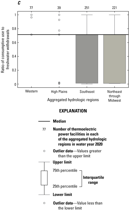
Model estimates of thermoelectric-power (A) withdrawals from fresh water and saline water and (B) ratio of consumptive use to freshwater withdrawals; and (C) boxplot showing ratio of consumptive use to freshwater withdrawals at the powerplant scale in the conterminous United States, water year 2020. Consumptive use was not estimated for thermoelectric plants that use saline water. Internal white lines in fig. 15A–15B indicate boundaries of hydrologic regions. Model estimates for thermoelectric-power water withdrawals and consumptive use are from Galanter and others (2023).
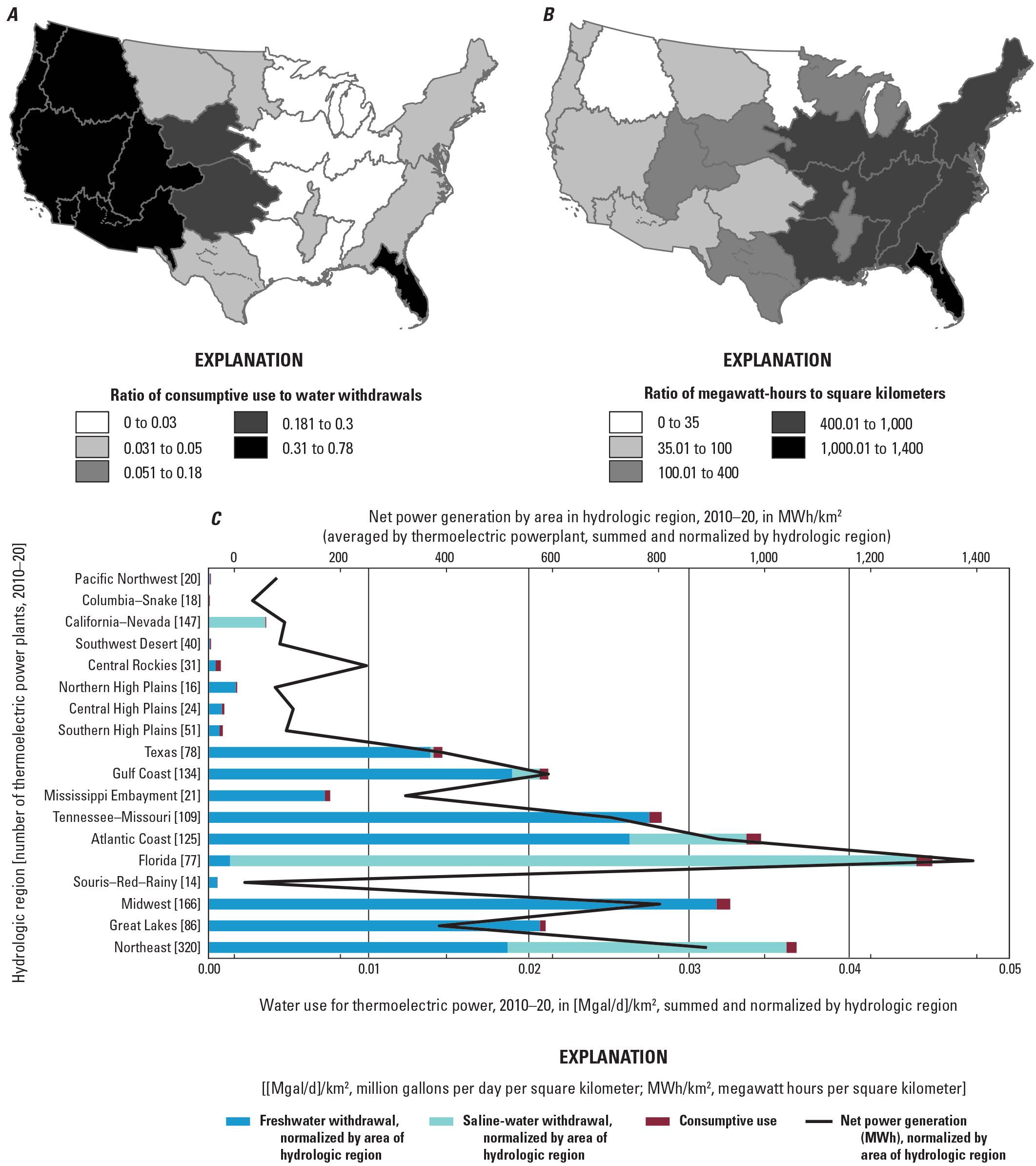
Model estimates for thermoelectric power, aggregated by hydrologic region, showing (A) ratio of consumptive use to freshwater withdrawals and (B) net power generation normalized by area (ratio of megawatt hours to square kilometers); and bar graph showing (C) net power generation (normalized by hydrologic region) and fresh water and saline-water withdrawals and consumptive use for thermoelectric power (normalized by area in each hydrologic region) in the conterminous United States, 2010–20. Net power generation is expressed in megawatt-hours and does not include data for facilities that receive water from municipal or reclaimed water sources. This figure is expressed in calendar years because net generation is only available in calendar years. Dark gray lines in fig. 16A–16B indicate hydrologic region boundaries. Model estimates for thermoelectric-power water withdrawals, consumptive use, and net power generation are from Galanter and others (2023).
Net power generation, a factor affecting thermoelectric water use, is greatest in the Eastern United States, particularly in the Florida, Atlantic Coast, and Northeast hydrologic regions, where thermoelectric withdrawals are greatest and where most of the country’s population resides (fig. 16B; Galanter and others, 2023). The Florida and Northeast hydrologic regions are also where withdrawals of saline surface water for thermoelectric power (on an absolute and normalized by area basis) are greatest (fig. 16C). Withdrawals from surface-water saline sources for thermoelectric power tend to be relatively large and consumptive use, not explicitly modeled for saline plants, is negligible because surface-water, saline-sourced plants often have once-through cooling systems (Galanter and others, 2023). Saline withdrawals are not relevant for freshwater-availability assessments.
As temperatures warm and the composition of the electrical grid changes in the United States, water use at thermoelectric powerplants will continue to change. The decrease in water withdrawals at thermoelectric powerplants can be largely attributed to a couple of trends. The share of total U.S. electricity generated by coal-fired plants (historically baseload powerplants using once-through freshwater cooling systems) is declining, and many of these plants are being retired; powerplants with once-through saline cooling systems are also being retired. Additionally, more of the electrical grid is being supplied by energy-efficient natural gas combined cycle plants paired with water-efficient recirculating cooling towers (Gorman Sanisaca and others, 2023). Conversely, thermoelectric consumptive use (the evaporative loss of water through the cooling system), which is sensitive to ambient water temperatures (once-through cooling systems) and air temperatures (recirculating tower cooling systems), could increase in response to heat waves and warming climates (Diehl and Harris, 2014).
Groundwater and Surface-Water Withdrawals from Fresh Water
Across the CONUS, the source of water—whether groundwater, surface water, public supply, reclaimed wastewater, or a combination thereof—typically depends on the availability of these sources and on the category of use. This section focuses on freshwater withdrawals; saline water withdrawals are discussed in section, “Thermoelectric Power Withdrawals and Consumptive Use,” where they are most relevant. On average during water years 2010–20, about 62 percent of water withdrawals for public supply, crop irrigation, and thermoelectric power were from surface water and 38 percent of withdrawals were from groundwater (table 4). Crop irrigation and thermoelectric power dominate water use across the country, but not in the same way everywhere.
Estimated water use for water year 2020 is summarized in figure 17, with 2020 representing a different time period than the values in tables 1–7 (although relative volumes are similar). Most surface-water withdrawals occur in the Western aggregated hydrologic regions for crop irrigation and in the Southeast and Northeast through Midwest aggregated hydrologic regions for thermoelectric power (fig. 17). Most groundwater withdrawals occur in the Western and High Plains aggregated hydrologic regions for crop irrigation. Sources of water for public supply are mixed: (1) more surface water is used than groundwater in the Eastern United States, (2) groundwater is the dominant source in the Western aggregated hydrologic regions, and (3) withdrawals from both surface-water and groundwater resources are nearly equal in the High Plains hydrologic region. Withdrawals from groundwater and surface water for crop irrigation are nearly the same in the Western aggregated hydrologic regions and withdrawals from groundwater are nearly three times those from surface water in the High Plains aggregated regions.
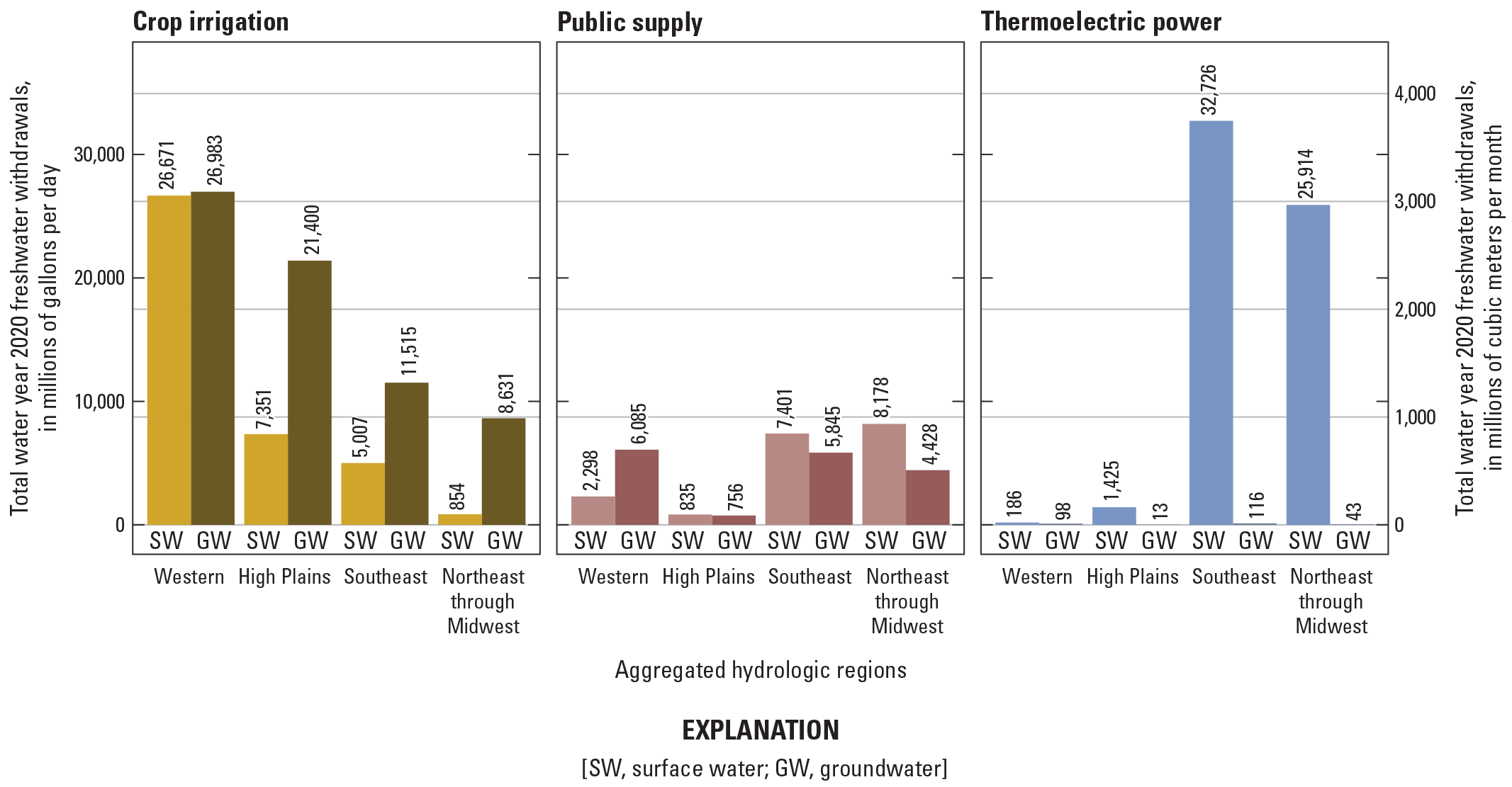
Model estimates of sources of total freshwater withdrawals for aggregated hydrologic regions in the conterminous United States, water year 2020. Numbers on the bars do not match values in tables 1–7, which indicate averages for water years 2010–20. Model estimates for crop irrigation, public supply, and thermoelectric-power sources of water withdrawals are from Haynes and others (2024), Luukkonen and others (2023), and Galanter and others (2023), respectively.
Patterns of predominant water withdrawals from surface water compared to groundwater across the CONUS in water year 2020 are shown for public supply, crop irrigation, and thermoelectric power in figure 18. Groundwater was the dominant source of water for public supply in many HUC12s in the United States, although surface water was the dominant source for large swaths in the Southeast and Northeast through Midwest aggregated hydrologic regions. For crop irrigation, large parts of several hydrologic regions—including the Central and Southern High Plains, Texas, the Mississippi Embayment, Florida, and the California–Nevada hydrologic regions—use groundwater primarily from the High Plains, the Mississippi River Valley alluvial, the Floridan, and the Central Valley (California) aquifer systems for crop irrigation. These important aquifer systems are undergoing substantial volumes of groundwater depletion, which contribute to saltwater inland migration (Konikow, 2015; Bellino and others, 2018). In contrast, the Columbia–Snake, Northern High Plains, and Central Rockies hydrologic regions use more surface water than groundwater for crop irrigation.
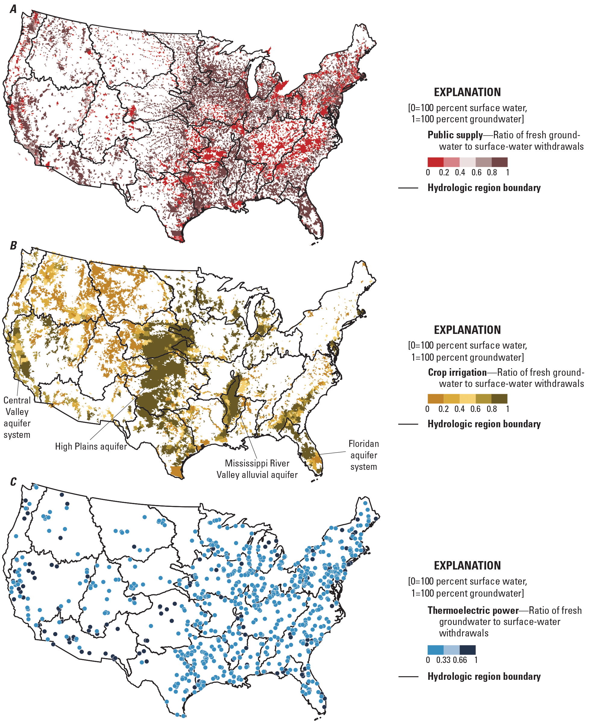
Model estimates of ratios of fresh groundwater to surface-water withdrawals for (A) public supply, (B) crop irrigation, and (C) thermoelectric power in the conterminous United States, water year 2020. The public supply and crop-irrigation maps show information for 12-digit hydrologic unit codes (HUC12s), whereas the thermoelectric map shows symbols for powerplants because the 1 percent of HUC12s with thermoelectric powerplants are too small to be visible at the CONUS scale. Dots for the thermoelectric maps are positioned at the centroids of HUC12 polygons in which facilities are located. Model estimates for public supply, crop irrigation, and thermoelectric-power sources of water withdrawals are from Luukkonen and others (2023), Haynes and others (2024), and Galanter and others (2023), respectively.
Most thermoelectric facilities in the eastern half of the country use predominantly fresh surface water for cooling; in the western half of the country, a larger proportion of thermoelectric facilities use groundwater (fig. 18). As described in section, “Thermoelectric Power Withdrawals and Consumptive Use,” differences in thermoelectric plant cooling systems between eastern and western States contribute to this geographic pattern of water source for thermoelectric power. Withdrawals for thermoelectric power from saline or other sources are not shown in figure 19; facilities that use saline water are located primarily along the eastern coastline, with a few facilities in California (fig. 15A; Galanter and others, 2023).
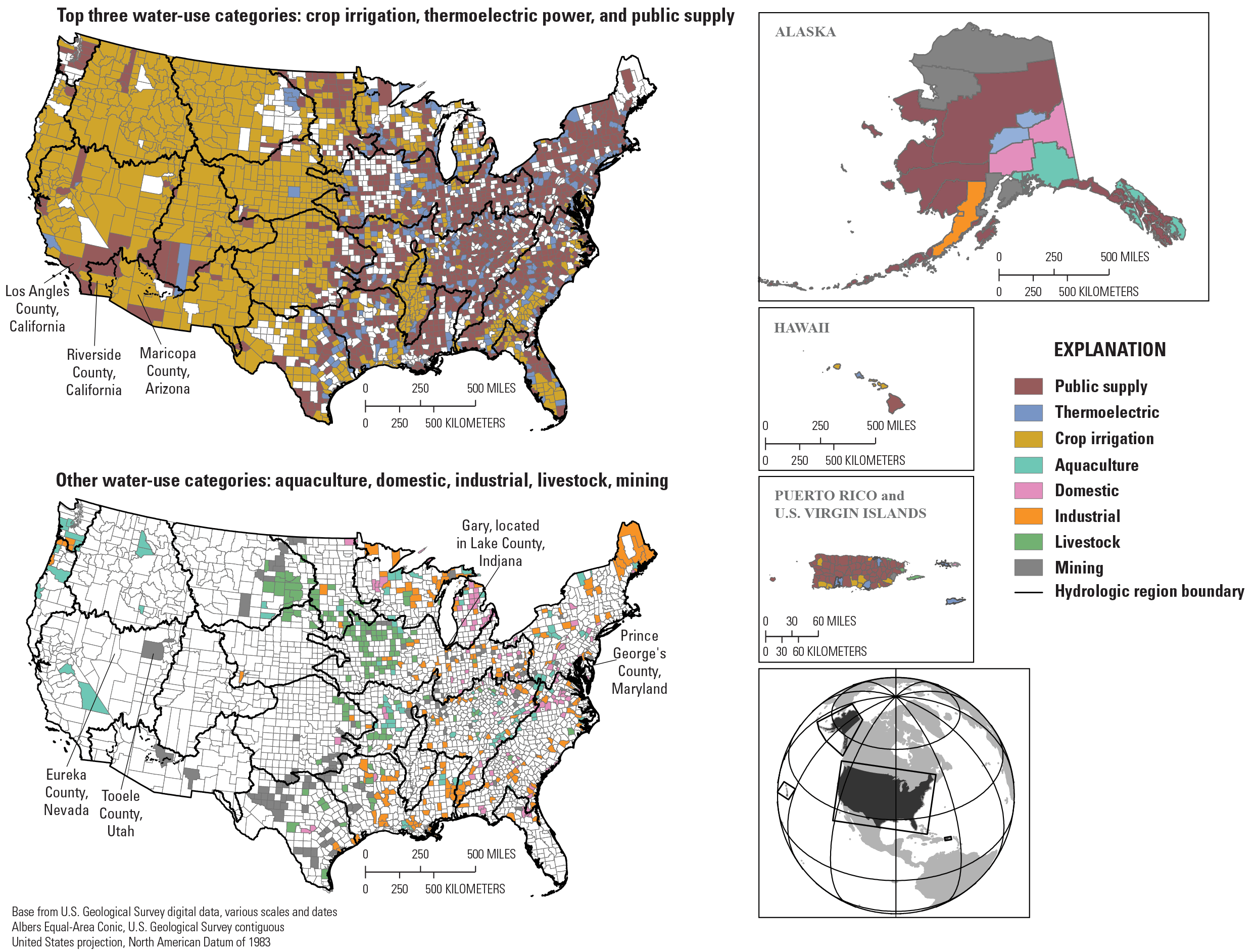
Categories of water use by county where the given category was the single largest category of water withdrawal, including fresh water and saline water, in the conterminous United States, Alaska, Hawaii, and Puerto Rico, for 2015. Commercial water use is not included because the U.S. Geological Survey has not estimated it since 1995. Estimates of the top category of county water use are from Houston and others (2022). Figure is modified from Casarez and others (2023).
Water Use Estimated Using Previous USGS Approaches—2015 Estimates
The water-use categories of self-supplied industrial, self-supplied domestic, self-supplied mining, self-supplied livestock, and self-supplied aquaculture together accounted for 10 percent of water withdrawals in the United States in 2015 (Dieter and others, 2018a). Although a small proportion nationally, these water-use categories can be locally important and therefore are included in a comprehensive representation of national water use. Because models for these categories are still in development as of the date of this report (2024), information from the most recent water-use reports (2010 and 2015) is presented in this chapter (Maupin and others, 2014; Dieter and others, 2018a). Commercial water use has not been included in USGS estimates of water use since 1995 and is not one of the eight categories to be modeled; it is discussed in this section using the most recent estimates available (1995) because it was historically reported as a separate category of use (Solley and others, 1998). The 2015 and other historical water-use estimates presented in this chapter show annual values on the basis of calendar years, reflecting the published data, whereas most depictions of modeled water use estimates in this publication are presented on the basis of water years (October through September), to provide information consistent with other chapters of this publication.
Requirements for water—purposes and amounts, absolute and relative within a geographic area—vary considerably across the country. Each of the eight USGS water-use categories is locally the largest water user in at least a few counties in the United States (fig. 19). Consistent with modeled estimates presented in this chapter, 2015 irrigation estimates overwhelmingly accounted for the largest water withdrawals for most counties in the western half of the country and in a few other areas such as the Mississippi Embayment and Florida hydrologic regions. Like modeled estimates, public supply also was most frequently the largest category of water use in the Eastern United States, and counties dominated by thermoelectric water use were interspersed throughout the eastern part of the country. Nearly any county with at least one thermoelectric powerplant with a once-through cooling system has thermoelectric power as the dominant category of water use.
In 2015, total water withdrawals in the United States were 281,000 Mgal/d from fresh water, 41,000 Mgal/d from saline water, and 322,000 Mgal/d from all water sources (Dieter and others, 2018a). Withdrawals in the CONUS were 279,000 Mgal/d from fresh water, 38,700 Mgal/d from saline water, and 317,700 Mgal/d from all water sources. The categories of public supply, irrigation (which in 2015 included water to irrigate crops, golf courses, parks, and all other landscape watering), and thermoelectric power represented 90 percent of total water withdrawals in 2015. The same percentage is applicable whether the context is the CONUS, or outside the CONUS, total fresh water, or total fresh water plus saline water. Withdrawals for industrial use represented about 5 percent of fresh water and total withdrawals. Withdrawals for aquaculture represented about 2.7 and 2.3 percent of fresh water and total withdrawals, respectively. Withdrawals for domestic and livestock, all fresh water, and mining (47 percent of which was fresh water and 53 percent of which was saline water) each represented about 1 percent of freshwater and total withdrawals.
Self-Supplied Industrial Withdrawals and Total Industrial Water Use
In 2015, withdrawals from fresh water for self-supplied industrial use were 14,000 Mgal/d and accounted for about 5 percent of total freshwater withdrawals in the United States (Dieter and others, 2018a). In 2015, 786 Mgal/d also were withdrawn from saline sources for industrial use, accounting for 2 percent of total saline withdrawals. Groundwater was the source of 2,670 Mgal/d and surface water the source of 11,300 Mgal/d of freshwater withdrawals for industrial use (19 percent and 81 percent, respectively). The USGS did not estimate public-supply deliveries to industrial water users in 2015. The most recent estimate of industrial deliveries was made in 1995, when deliveries were about 19 percent of total industrial water use, self-supplied withdrawals were 81 percent of total industrial water use, and deliveries to industrial users represented about 12 percent of total withdrawals for public supply (Solley and others, 1998).
Indiana and Louisiana in 2015 together accounted for 32 percent of withdrawals from fresh water for industrial use in the country, with Lake County, Indiana, (which includes the city of Gary) accounting for 52 percent of Indiana’s industrial freshwater withdrawals (Dieter and others, 2018b). This single county also accounted for 8 percent of total industrial freshwater withdrawals in the country. Leading sectors that contributed to industrial water use in Indiana were automotive, pharmaceuticals, and steelmaking; in Louisiana, these sectors were petroleum refining, chemicals, and petrochemicals. Throughout most of predominantly rural Maine, industrial use accounted for more water use than all other categories in 2015 (fig. 19), primarily because of water demand from the pulp and paper industry.
Self-Supplied Domestic Withdrawals and Total Domestic Water Use
Nationwide in 2015, domestic water users received most of their water from public suppliers. Eighty-eight percent (23,300 Mgal/d) of water used for domestic purposes came from public suppliers and 12 percent (3,260 Mgal/d) were self-supplied (Dieter and others, 2018a). Domestic self-supplied withdrawals accounted for about 1 percent of total withdrawals in the United States in 2015. Of the 3,260 Mgal/d of self-supplied withdrawals for domestic use, the source for 49.1 Mgal/d (2 percent) was surface water and for 3,210 Mgal/d (98 percent) was groundwater.
Domestic water use (also referred to as residential or household water use) is water used for indoor household purposes such as drinking; food preparation; bathing; washing clothes and dishes; flushing toilets; and outdoor purposes such as watering lawns and gardens, washing vehicles, and filling pools. Domestic self-supplied water users usually live where public water suppliers are not available (that is, outside cities, metropolitan areas, and towns), although some populations in urban or suburban areas are self-supplied and some rural populations are served by small public suppliers.
Estimates for domestic water use directly relate to population. For historical USGS water-use estimates, the population of domestic self-supplied water users was typically estimated as the difference between total county population and the population served by public suppliers (Dieter and others, 2018a), sometimes adjusted based on local understanding of factors such as population distribution for multi-county public supply systems and seasonal shifts in population. Self-supplied population was multiplied by a Statewide or countywide per-capita residential water-use coefficient, which, in 2015, was usually extrapolated from reported data or carried over from previous estimates (Luukkonen and others, 2021). In 2015, per-capita coefficients for domestic self-supplied use ranged from 36 gallons (gal) per capita per day in Connecticut to 186 gal per capita per day in Nevada, with a national average of 77 gal per capita per day (Dieter and others, 2018a).
States with total domestic use (the combination of public-supply deliveries to domestic users and self-supply domestic use) greater than 1,000 Mgal/d in 2015 were California, Texas, Florida, New York, and Illinois (Dieter and others, 2018a). States with the largest self-supplied withdrawals for domestic use were Pennsylvania, Michigan, and New York. On a per-capita basis, the largest total domestic water use occurred in Idaho, Utah, Arizona, and Hawaii. Prince George’s County in Maryland was the county with the largest self-supplied domestic population and withdrawals (0.7 percent of the national total). The county with the largest volume of public-supply deliveries to domestic users was Los Angeles County, California (3.5 percent of the national total). Virginia and Michigan have the most counties where domestic self-supplied use is larger than any other category of water use (fig. 19; Dieter and others, 2018b) .
Self-Supplied Commercial Withdrawals and Total Commercial Water Use
Commercial water use (self-supplied withdrawals plus deliveries from public supply) was most recently compiled nationwide in 1995, when it represented about 3 percent of total freshwater use (Solley and others, 1998). Self-supplied withdrawals for commercial use (all fresh water) were 2,890 Mgal/d and deliveries to commercial water users from public supply were 6,690 Mgal/d. Withdrawals for self-supplied commercial use accounted for less than 1 percent of total freshwater withdrawals in the United States in 1995. Groundwater was the source of 939 Mgal/d and surface water the source of 1,950 Mgal/d of freshwater withdrawals for commercial use (32.5 percent and 67.5 percent, respectively).
Commercial water use includes water used for motels, hotels, restaurants, office buildings, other commercial facilities, military and nonmilitary institutions, and (for 1990 and 1995) offstream fish hatcheries. In 1995, California, Oregon, and New York had the largest total commercial use, and Oregon, California, and Idaho had the largest self-supplied withdrawals for commercial water use (Solley and others, 1998). Although a few State agencies furnished data from reported or permitted withdrawals for commercial water use to the USGS for the 1995 water-use report, most States estimated commercial withdrawals from coefficients related to the particular type of commercial establishment, such as the number of students at a university, workers in an office building, or beds in a hotel or hospital.
Self-Supplied Livestock Water Use
Withdrawals for livestock water use, all from fresh water, were 2,000 Mgal/d and accounted for less than 1 percent of total freshwater withdrawals in the United States in 2015 (Dieter and others, 2018a). About 62 percent (1,240 Mgal/d) of withdrawals for livestock water use were from groundwater and 38 percent (760 Mgal/d) were from surface water.
The livestock category is defined as water used for livestock watering, feedlots, dairy operations, and other on-farm needs and does not include water used to grow feed crops. Types of livestock include dairy cows and heifers, beef cattle and calves, sheep and lambs, goats, hogs and pigs, horses, and poultry. About 14 percent of total water withdrawals for livestock in the United States in 2015 occurred in Texas, with California and Iowa combined contributing another 17 percent. A large part of withdrawals for livestock were for cattle (Dieter and others, 2018a). Livestock water withdrawals are typically estimated using county-level animal population data provided by the U.S. Department of Agriculture Census of Agriculture, produced every 5 years, and average water-use coefficients, in gallons per head per day, for each animal type (Lovelace, 2009b).
Self-Supplied, Mining-Water Use
Water used for mining in the United States includes fresh water and saline water. In 2015, withdrawals for mining from fresh water were 1,880 Mgal/d and from saline water were 2,120 Mgal/d, accounting for less than 1 percent and 5 percent of total withdrawals in the U.S. for fresh water and saline water, respectively (Dieter and others, 2018a). About 54 percent (1,010 Mgal/d) of withdrawals from fresh water for mining were from groundwater and 46 percent (877 Mgal/d) were from surface water. About 88 percent (1,860 Mgal/d) of withdrawals from saline water for mining water use were from groundwater and 12 percent (256 Mgal/d) were from surface water.
Mining water use includes water used for the extraction of naturally occurring minerals including solids (such as coal, sand, gravel, and ores), liquids (such as crude petroleum), and gases (such as natural gas). It includes uses associated with quarrying, milling of mined materials, injection of water for secondary oil recovery or for unconventional oil and gas recovery (such as hydraulic fracturing), and other operations associated with mining activity.
The largest withdrawals of fresh water for mining were in Nevada (10 percent of the U.S. total). Eureka County, Nevada (fig. 19) used 77.4 Mgal/d of fresh water in 2015 for mining, with primary products of silver and gold, and other ores such as lead, copper, and zinc (Burger and others, 2018; Muntean and Micander, 2023). Eureka County accounted for 4.3 percent of total mining withdrawals from fresh water in the country and 40 percent of withdrawals for mining in Nevada in 2015. Tooele County, Utah (fig. 19), had the largest total county scale withdrawal from mining that included saline water of 131.4 Mgal/d in 2015. Texas, Florida, Ohio, and Indiana each had similar withdrawal volumes of about 130 Mgal/d and together accounted for 27 percent of freshwater withdrawals for mining nationwide. More than 200 Mgal/d of saline water were withdrawn for mining in Texas, California, and Utah.
Self-Supplied, Golf-Course-Irrigation Water Use
In the 2015 and previous USGS water-use reports, irrigation water use included water used for crops and recreational land including golf courses. USGS staff who provided State-based information for the national water-use reports had the option of either differentiating golf-course-irrigation water use from crop irrigation or of reporting the two types as a single value. Based on information from 36 States that reported golf-course irrigation separately from crop irrigation, withdrawals for golf-course water use accounted for less than 1 percent of irrigation withdrawals in the United States in 2015 (Dieter and others, 2018b). Reported withdrawals for golf-course irrigation totaling 1,039 Mgal/d were all from fresh water and accounted for less than 1 percent of total freshwater withdrawals in the United States in 2015 (Dieter and others, 2018b). About 47 percent (488 Mgal/d) of withdrawals for golf-course-irrigation water use were from groundwater and 53 percent (551 Mgal/d) were from surface water.
In the States with reported golf-course-irrigation use, Maricopa County, Arizona (fig. 19), had the largest total withdrawal from fresh water for golf-course irrigation (83.8 Mgal/d; 58 percent from groundwater and 42 percent from surface water) by almost three times the next largest county, Riverside County, California (29.3 Mgal/d; 69 percent from groundwater and 31 percent from surface water; fig. 19). Maricopa County also used the largest amount of reclaimed wastewater for golf-course irrigation (25 Mgal/d or 23 percent of total golf-course-irrigation water use) and had the largest consumptive use for golf-course irrigation (87 Mgal/d) of all counties in the country with reported use. Florida, California, and Arizona had the largest statewide withdrawals for golf-course irrigation and accounted for a total of 43 percent of golf-course withdrawals for reporting States. These States also had the largest amounts of reclaimed wastewater and consumptive use for golf-course irrigation. Ninety-nine percent of golf-course irrigation used sprinkler types of systems; the remaining 1 percent used micro irrigation or surface (flood) irrigation methods (Dieter and others, 2018b).
Other Water-Use Topics
Water Use for Energy Production
Water withdrawals for energy production, not historically reported as a separate category of water use by the USGS, include withdrawals for thermoelectric water use plus water withdrawals for mining operations that produce fuels to generate electricity, such as coal, uranium, and oil and gas, and any industrial processing of the mined products. Water-withdrawal estimates for energy production in this chapter do not distinguish between mining and industrial processing functions of production.
Published information from the Energy Information Administration (EIA) about coal production in the United States indicates that 535.4 million short tons were produced in 2020 from 22 States (U.S. Energy Information Administration, 2022a). This was the smallest amount of coal produced during 2010–20; the largest amount during that period was 1,096 million short tons in 2011. States with the most coal production in 2020 were Wyoming, West Virginia, and Pennsylvania. Water needs for coal production, related to whether the mining operation is surface or underground, includes water for coal cutting in underground mines, dust suppression for mining and hauling activities, and revegetation (U.S. Department of Energy, 2006). Water demand for coal mining might include water pumped to relieve pressure and prevent heaving of the mine if located near a confined aquifer (Reedy and Scanlon, 2022).
Water use for coal production in the United States is not reported to the EIA or any other Federal agency. Lovelace (2009a) published estimates of 50 and 59 gallons as the minimum and maximum volumes of water, respectively, needed to produce one short ton of crude coal ore. A more recent coefficient based on 2020 data reported to the Texas Water Development Board is 69 gallons per short ton of coal ore (Reedy and Scanlon, 2022). Applying the Texas coefficient to total coal production in the United States in 2020 provides an estimated water use of 101.2 Mgal/d for coal mining.
The EIA also publishes information about uranium concentrate production in the United States. The total number of uranium concentrate processing facilities in the United States from 2010 to 2020 ranged from 4 to 7; there were 6 facilities in 2020 (U.S. Energy Information Administration, 2022b). Most of these facilities were in situ recovery plants and a small number were mills. Over the lifetime of a uranium mine, water is used for production and subsequent restoration of the groundwater resource. For four in situ recovery mines in Texas with uranium production and mining and restoration water-use information, Gallegos and others (2022, tables 1) estimated that lifetime water use ranged from 491 to 1,312 million gallons (over 4,399–10,051 days of operation, averaging 0.11 Mgal/d). Applying this average as a coefficient to the six operational in situ recovery mines operating in 2020, about 0.66 Mgal/d of water was used for uranium production in 2020. About 54–77 percent of lifetime water use was for restoration (post-production). Because no source of information exists for the number of uranium mining facilities in restoration rather than mining mode of operation, the estimate of 0.66 Mgal/d for uranium mining, not including restoration water use, underestimates the total.
Hydraulic fracturing, or fracking, is the process of injecting water, sand, and (or) chemicals into a well to break up underground bedrock and free up oil or gas reserves. About 40,000 gal of water were used on average in 2020 for hydraulic fracturing of a single well (Groundwater Protection Council and U.S. Department of Energy, 2023); in 2019, annual water use per well was about 17 Mgal of water (Valder and others, 2021). More water is used for extractions from continuous oil and gas reservoirs (deposits that are distributed evenly throughout the geologic formation) than from conventional oil and gas reservoirs (discrete deposits). In the Permian Basin (Texas and New Mexico), which is becoming one of the world’s largest continuous oil and gas resources, annual water use for continuous oil and gas mining has increased from 0.587 to 16.9 Mgal per well during 2010–19 (Valder and others, 2021). The large water volumes required for this mining activity have particular importance because of the semiarid climate, growing population, and limited availability of water resources in the basin. In 2020, 19 states (including Alaska) reported 7,930 fracked wells that used a total of 317 Mgal/d of water (Groundwater Protection Council and U.S. Department of Energy, 2023). Excluding data for Alaska in order to compare to the other energy sectors, 7,921 wells were fracked and the associated water use remained 317 Mgal/d. Other processes that produce oil and gas besides hydraulic fracturing (such as enhanced oil recovery, oil shale and oil sands extraction, or waterflooding) are not accounted for in this analysis.
Modeled fresh water and saline water used for thermoelectric power in 2020—80,433 Mgal/d (Galanter and others, 2023)—was 99 percent of the 2020 estimated total water use for energy production from this analysis (80,852 Mgal/d). Water withdrawals in 2020 for oil and gas production were estimated at 317 Mgal/d (0.5 percent), for coal production were 101.2 Mgal/d (0.2 percent), and for uranium mining were 0.7 Mgal/d (less than 0.1 percent; fig. 20).
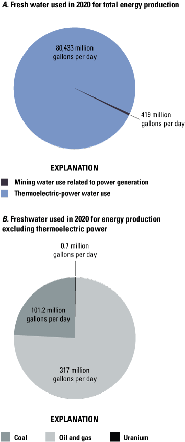
Estimates of fresh water used for (A) total energy production and (B) energy production excluding thermoelectric power in the conterminous United States plus Alaska, 2020. Model estimates for thermoelectric-power withdrawals are from Galanter and others (2023); coal production data are from the U.S. Energy Information Administration (2022a); coal water-use coefficient based on production is from Reedy and Scanlon (2022); uranium production and water-use data are from Gallegos and other (2022; and oil and gas water-use data are from the Groundwater Protection Council and U.S. Department of Energy (2023).
Water Reuse
Reuse of water is the practice of reclaiming water from various sources, treating it, and reusing it for beneficial purposes. In some parts of the country, reused water is a substantial component of water use and could be an important element to consider for water-availability assessments because it deviates from the basic conceptual model of “withdrawal to use” and “use to return flow” in the water cycle. In the traditional wastewater model, public or industrial effluent is discharged into streams and is a part or all of the streamflow that sustains instream ecological function. This effluent, mixed with natural flow, is available for withdrawal downstream of the discharge point for various potable and non-potable uses. Streamflow in arid and semi-arid regions—particularly in urbanized watersheds—can be dominated by effluent (Brooks and others, 2006).
Water reuse disrupts the traditional wastewater model where some or all of the effluent that previously would have been discharged to a stream is intercepted, treated further if necessary, and used for various purposes that may include potable reuse. Some States have extensive programs in place or planned for reusing water, as do several organizations and national agencies. The Bureau of Reclamation has provided more than $761 million in grant funding to projects since 1992 that reclaim and reuse wastewater and impaired groundwater and surface water (Bureau of Reclamation, 2021). Since 2020, the U.S. Environmental Protection Agency has been actively fostering collaborations and promoting and funding water reuse infrastructure and research grants for industrial reuse, onsite non-potable reuse, stormwater capture and use, and agricultural reuse for local and nationwide projects (U.S. Environmental Protection Agency, 2023).
In 2015, 4.6 percent of water withdrawals (saline water plus fresh water) and 11 percent of freshwater withdrawals in Florida (percentages calculated by adding reclaimed wastewater use to withdrawals) were reclaimed wastewater; most of this was used for urban and agricultural irrigation and industrial use (Marella, 2020). Nationwide reclaimed wastewater in 2015 accounted for 0.5 percent of irrigation water use with most in California, Arizona, and Florida (Dieter and others, 2018a). In water year 2020, reclaimed wastewater accounted for 0.2 percent of thermoelectric water use in 22 States (Galanter and others, 2023). The East Bay Municipal Utility District, whose wastewater system serves about 740,000 people along the eastern shore of the San Francisco Bay in California, has set a water reuse goal of 20 Mgal/d by 2040 for irrigation, office-building toilet flushing, and thermoelectric and industrial cooling towers (East Bay Municipal Utility District, 2019).
The oil and gas industry actively promotes beneficial reuse of produced water, which is water that comes out of oil and gas wells along with crude oil during oil production (Groundwater Protection Council, 2023). Because volumes of produced water can be substantial and of highly variable chemical composition (typically containing oil and other organics, suspended and dissolved solids, and other chemicals), often costly treatment is required before disposal. However, water scarcity in some areas incentivizes the reuse of this water. Options for beneficial reuse of produced water include hydraulic fracturing, irrigation, industrial, and public-supply water use, surface-water discharge to maintain streamflow, and groundwater recharge. In Texas, about 10 percent of water used for hydraulic fracturing in the Permian Basin is reused produced water (Reedy and Scanlon, 2022).
Bottled Water
The USGS is assessing the hydrologic impacts of water withdrawals for bottling on water tables, on concentrations of contaminants, and on saltwater intrusion into the groundwater, and to better understand water availability (sidebar 3).
Sidebar 3. Bottled Water (by Cheryl A. Dieter)
With the U.S. bottled water market at 14.4 billion gallons in 2019 (fig. S3.1), bottled water is the largest beverage category by volume in the country, nearly all of which is sourced domestically (Beverage Marketing Corporation, 2020). The goal of this project is to improve understanding of the potential hydrologic and socioeconomic impacts of the bottled water industry nationally and to develop tools that can be used to assess those impacts in the future as the bottled water industry, climate, hydrologic conditions, and (or) socioeconomic conditions change.
The U.S. Geological Survey is using multiple approaches to understand impacts of the water bottling industry on water availability including (1) a national inventory of bottling facilities, facility characteristics, and where available, water withdrawals (Buchwald and others, 2023); (2) focused regional assessments throughout the United States to better understand impacts of water bottling facilities in terms of water table, saltwater intrusion, and (or) water quality conditions; and (3) national assessments and analysis.
The regional assessments are all unique and use existing models and data to evaluate hydrologic responses and implications of responses to regional hydrologic systems. However, a systematic assessment of hydrologic conditions, economic factors, and social consequences of water withdrawals for bottling will provide a comparison of the various regional assessment locations.
The national assessments will aim to (1) provide a national context of water-bottling-facility withdrawals on other national water uses; (2) assist in evaluating the impacts of the water-bottling industry on communities and ecosystems using the national inventory and other social, economic, and environmental data; (3) determine potential impacts associated with change in growth of the bottled-water industry; and (4) help us to understand the role of the industry during and after short- and long-term emergency events where communities rely on bottled water for drinking-water needs.
Bottled water. Photograph by U.S. Geological Survey.
Interbasin Transfers
Interbasin transfers, or the movement of water across the landscape in constructed conveyances (in other words, pipes, canals, aqueducts, tunnels), must be integrated into national water-availability assessments because the volumes involved in these water transfers can substantially alter natural flow regimes (Emanuel and others 2015; Liu and others, 2022). Increases or decreases in water supplies caused by interbasin transfers will be missed if they are not deliberately accounted for. Interbasin transfers are constructed and operated to move water from one basin to another basin that has unmet water needs for a specific purpose, such as public supply, irrigation, navigation, flood management, or a combination of these uses.
The scale at which an interbasin transfer is defined is an important consideration for water-availability assessments. Many conveyances of water across small sub-watershed boundaries for tributary systems such as HUC12s are not interbasin transfers across larger basin delineations, such as subbasin or subregion boundaries (8-digit and 4-digit hydrologic unit codes [HUC8s or HUC4s, respectively]). Governing bodies that regulate or oversee water transfers carefully delineate the scale of basins within their purview. For example, the Delaware River Basin Commission defines interbasin transfers as movement across HUC4 boundaries. Smaller conveyances are typically associated with irrigation, particularly in the Western United States, or with public supply, whereas larger conveyances that cross HUC8 or HUC4 boundaries are often constructed for multiple uses and if they cross state boundaries, are managed by regional or interstate commissions. The degree to which interbasin transfers need to be managed depends to a large extent on the size of the project and need for coordination among competing interests. In the Western United States, interbasin transfers and all human-induced movement of water is subject to water rights doctrines based on prior appropriation and beneficial use. Many agreements were made based on historical climate conditions and water needs and do not have built-in capacity to adapt to changes in climate and water demand (Hedden-Nicely, 2022).
Energy and engineering are required to convey water across a basin divide—energy to pump water over a divide and engineering to construct tunnels or pipes through a divide. In some parts of the country, substantial volumes of water are moved tens or hundreds of miles, involve multiple reservoir systems and conveyances, and can cross watershed boundaries as large as the Continental Divide (fig. 21). Examples of such interbasin transfers include the following:
-
• For the Denver Water system, water is transported as far as 250 miles (mi) from reservoirs located west of the Continental Divide in Colorado through tunnels and canals to provide water for municipal and industrial use, hydroelectric power, and recreation in Denver, Colorado, and the surrounding areas.
-
• With a system of reservoirs, tunnels, and aqueducts that spans 125 mi, the New York City water supply system provides more than 1 billion gallons of drinking water to nearly 10 million residents in the New York City metropolitan area every day.
-
• The California State Water Project provides water to 27 million Californians and 750,000 acres of farmland in a system of 36 storage facilities, 26 dams, 21 pumping plants, 5 hydroelectric powerplants, and about 700 mi of canals, tunnels, and pipelines (California Department of Water Resources, 2022).
-
• The Central Arizona Project delivers more than 450 billion gallons of water each year from the Colorado River across 336 mi of desert through tunnels and canals to industrial, public supply, agricultural, and Tribal customers in three counties in Arizona, serving more than 80 percent of the State’s population (Witcher, 2022).
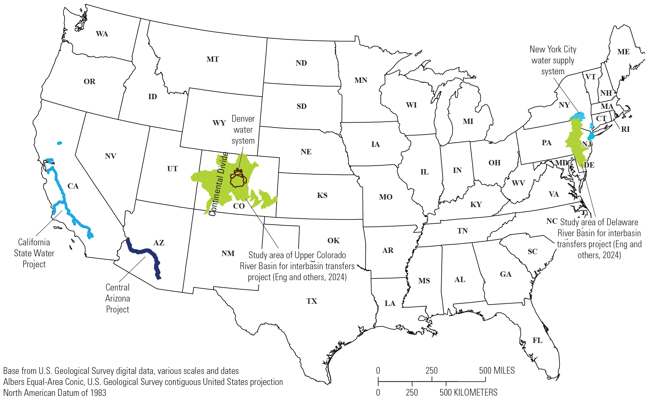
Selected large interbasin transfer projects in the conterminous United States. States are indicated with two-digit postal codes. Study areas for the Delaware and Colorado River Basins are from Eng and others (in press).
Interbasin transfers of water can have a substantial effect on hydrology and water availability in sending and receiving basins and are crucial to the understanding of water budgets (Evenson and others, 2018); however, comprehensive quantitative information about interbasin flows is not available. Limited data exist to inform models for interbasin transfers in the United States. Building on earlier work, Dickson and Dzombak (2017) assembled an inventory of 2,161 water transfers crossing 6-digit hydrologic unit code (HUC6) boundaries. The Siddik and others (2022) inventory of transfers crossing HUC4 boundaries was the first to assemble and publish available flow data for water transfers. An inventory by Dobbs and others (2023) provides flow data for 599 surface-water interbasin transfers in the United States, focusing on those associated with public supply in the CONUS. Large interbasin transfers are generally gaged to ensure compliance with detailed allocation requirements in management plans and compacts, although flow data might not be available to the public if they are considered sensitive information. Compared to other types of hydrologic models, models for interbasin transfers present a unique challenge because transfers reflect human influences independent of hydrologic and climate factors.
With the goal of identifying features related to interbasin transfers that can be integrated in national water-availability assessments, the USGS used machine-learning methods to model transfers of water between medium-size watersheds (HUC8) in two study areas, the upper Colorado River Basin and part of the Delaware River Basin (Eng and others, in press; fig. 21). Researchers reported that when grouped by similar types of purposes (for example, for public supply or irrigation), interbasin transfers have some generalizable characteristics related to seasonality and that certain flow characteristics related to water transfers can be predicted at unmonitored locations for some months or seasons of the year. In Eng and others (in press) work, the biggest limitations for predicting flow characteristics of interbasin transfers of water were the lack of interbasin transfer flow data in many parts of the country and lack of spatially and temporally suitable water-use estimates to inform the models. The modeling approaches of the USGS water-use program that began in 2020 to prod uce near real-time estimates of future and historical water use at the HUC12 scale will address the latter data need.
Summary and Conclusions
This chapter provides an analysis of public supply, crop irrigation, and thermoelectric power water use in the conterminous United States (CONUS) for the water years 2010–20, with a focus on estimates for water year 2020 (October 1, 2019–September 30, 2020). These three categories of water use account for about 90 percent of water withdrawals in the United States. The values presented here are based on modeling approaches that estimate water use at temporal (monthly) and spatial scales (12-digit hydrologic unit code—small watershed scale or HUC12) compatible for integration into a broader national assessment of water availability.
Water-use models, which are replacing the U.S. Geological Survey previous data compilation method, provide results for nationally consistent estimates of monthly and annual water use. Model output includes estimates of water withdrawals (water removed from a groundwater or surface-water source for use), consumptive use (water removed from the immediate water environment—for example, by evapotranspiration), and estimates by water source (groundwater and surface water, but also saline water, reclaimed wastewater, or public-supply water for thermoelectric power). Models improve understanding of factors that influence water use and provide more information to analyze trends, plan strategically, and identify and quantify vulnerability thresholds for adaptive water management.
An estimated 244,817 million gallons per day (Mgal/d; 28,677 million cubic meters per month [Mm3/mo]) were withdrawn annually on average within the CONUS during water years 2010–20 from fresh water and saline water for crop irrigation, public supply, and thermoelectric power, with shares of 43, 14.5, and 42.5 percent for each of these categories, respectively. In the same period:
-
• Estimated withdrawals and consumptive use for public supply were 35,400 and 4,219 Mgal/d (4,081 and 486 Mm3/mo), respectively;
-
• Estimated withdrawals and consumptive use for crop irrigation were 105,497 and 75,698 Mgal/d (12,147 and 8,716 Mm3/mo), respectively;
-
• Estimated withdrawals and consumptive use for thermoelectric power from fresh water were 82,656 and 2,904 Mgal/d (9,952 and 345 Mm3/mo), respectively; and
-
• Estimated withdrawals for thermoelectric power from saline water were 21,224 Mgal/d (2,497 Mm3/mo; consumptive use for saline water used by thermoelectric power facilities was not estimated).
Withdrawals for these categories of water use are highly spatially variable. Crop-irrigation water use dominates withdrawals in western States, whereas thermoelectric power water use dominates withdrawals in eastern States. Public supply accounts for the largest percentage of water use in several heavily populated northeastern States. Public-supply models show that lower per-capita use, higher water withdrawals, and higher consumptive use were evident in coastal areas in the Western United States and in most of the Eastern United States compared to inland western areas. Intra-annual and interannual variability of crop-irrigation withdrawals was largely a function of climatic influences such as precipitation and evaporative demand. Estimates of the ratio of modeled crop-irrigation consumptive use to irrigation withdrawals varied across the country, with largest ratios in the Northeast and smallest ratios in Western United States, with a national average of 72 percent.
Thermoelectric-power water use is characterized by large withdrawals and relatively low consumptive use, which means that most of the withdrawn water was returned to the local environment. Withdrawals for thermoelectric power and the number of power plants are greatest in the Eastern United States. Consumptive use of water for thermoelectric power was 4 percent of thermoelectric withdrawals from fresh water across the CONUS, with large variability depending on whether the cooling system was once-through (characterized by large withdrawals with small relative consumptive use) or recirculating cooling (characterized by small withdrawals with large relative consumptive use). Western States withdraw relatively little water for thermoelectric power plants because most facilities recirculate cooling water and use water from public supply, groundwater, or reclaimed wastewater.
Throughout the CONUS, reliance on groundwater instead of surface water depended on the availability of water sources and on the type of water use. For public supply, withdrawals from groundwater are generally greater than withdrawals from surface water in the Western aggregated hydrologic regions and withdrawals from surface water are generally greater in the Southeast and Northeast through Midwest aggregated hydrologic regions. Nationwide, the predominant source of water for crop irrigation is groundwater, with large parts of the Central and Southern High Plains, Texas, Mississippi Embayment, Florida, and California–Nevada hydrologic regions using groundwater primarily from the High Plains, the Mississippi River Valley alluvial, the Floridan, and the Central Valley (California) aquifer systems, respectively. Most thermoelectric power facilities in the eastern half of the CONUS use surface water from fresh water and saline sources, and most thermoelectric power facilities in the western half of the CONUS use groundwater.
Five additional water-use categories, all self-supplied, account for about 10 percent of total water use for the CONUS: industrial, domestic, mining, livestock, and aquaculture. Other water-use elements that can be locally or regionally important for water availability include water reuse and bottled water.
The modeled water-use estimates described in this chapter do not incorporate interbasin transfers, wherein water used in one basin originates from withdrawals in a different basin. Comprehensive quantitative information about interbasin transfers in the CONUS is not available and the current modeling capability is limited to selected areas.
References Cited
Alzraiee, A., Niswonger, R., Luukkonen, C., Larsen, J., Martin, D., Herbert, D., Buchwald, C., Dieter, C., Miller, L., Stewart, J., Houston, N., Paulinski, S., Valseth, K, 2024, Next generation public supply water withdrawal estimation for the conterminous United States using machine learning and operational frameworks: Water Resources Research, 60, 25 p., accessed July 25, 2024, at https://doi.org/10.1029/2023WR036632.
Bellino, J.C., Kuniansky, E.L., O’Reilly, A.M., and Dixon, J.F., 2018, Hydrogeologic setting, conceptual groundwater flow system, and hydrologic conditions 1995–2010 in Florida and parts of Georgia, Alabama, and South Carolina: U.S. Geological Survey Scientific Investigations Report 2018–5030, 103 p., accessed November 15, 2023, at https://doi.org/10.3133/sir20185030.
Beverage Marketing Corporation, 2020, U.S. bottled water market: International Bottled Water Association, accessed April 25, 2023, at https://bottledwater.org/bottled-water-market/.
Brooks, B.W., Riley, T.M., and Taylor, R.D., 2006, Water quality of effluent-dominated ecosystems—Ecotoxicological, hydrological, and management considerations: Hydrobiologia, v. 556, no. 1, p. 365–379, accessed May 23, 2023, at https://doi.org/10.1007/s10750-004-0189-7.
Bruce, B.W., Prairie, J.R., Maupin, M.A., Dodds, J.R., Eckhardt, D.W., Ivahnenko, T.I., Matuska, P.J., Evenson, E.J., and Harrison, A.D., 2018, Comparison of U.S. Geological Survey and Bureau of Reclamation water-use reporting in the Colorado River Basin (ver. 1.1, September 2019): U.S. Geological Survey Scientific Investigations Report 2018–5021, 41 p., accessed November 21, 2023, at https://doi.org/10.3133/sir20185021.
Buchwald, C.A., Luukkonen, C.L., Martin, G.R., Kennedy, J.L., Wilson, J.T., Hian, M.E., and Dieter, C.A., 2023, Inventory of water bottling facilities in the United States, 2023, and select water-use data, 1955–2022, U.S. Geological Survey data release, https://doi.org/10.5066/P90Z125H.
Bureau of Reclamation, 2021, Water reliability in the West—2021 SECURE Water Act Report: Prepared for the U.S. Congress by Bureau of Reclamation, Water Resources and Planning Office, Denver, Colorado, 60 p., accessed November 9, 2023, at https://www.usbr.gov/climate/secure/docs/2021secure/2021SECUREReport.pdf.
Burger, M.H., Bellora, J.D., Fernette, G.L., and San Juan, C.A., 2018, Mines, mineral occurrences, and mining districts in the Carlin area, Nevada: U.S. Geological Survey data release, accessed December 21, 2023, at https://doi.org/10.5066/F7KD1X3X.
California Department of Water Resources, 2022, Management of the California State Water Project, Bulletin 132-19: California Department of Water Resources, accessed September 27, 2023, at https://water.ca.gov/Programs/State-Water-Project/Management/Bulletin-132.
Casarez, I.R., Houston, N.A., Merriman, K.R., Chan, A.Y., Dieter, C.A., and York, B.C., 2023, Water-use data-gap analysis: U.S. Geological Survey Story Map, accessed September 19, 2024, at https://storymaps.arcgis.com/stories/c8e2d30f212149c28875d87325592d2e.
Chinnasamy, C.V., Arabi, M., Sharvelle, S., Warziniack, T., Furth, C.D., and Dozier, A., 2021, Characterization of municipal water uses in the contiguous United States: Water Resources Research, v. 57, no. 6, 18 p., accessed December 13, 2023, at https://doi.org/10.1029/2020WR028627.
Dickson, K.E., and Dzombak, D.A., 2017, Inventory of interbasin transfers in the United States: Journal of the American Water Resources Association, v. 53, no. 5, p. 1121–1132, accessed December 15, 2020, at https://doi.org/10.1111/1752-1688.12561.
Diehl, T.H., and Harris, M.A., 2014, Withdrawal and consumption of water by thermoelectric power plants in the United States, 2010: U.S. Geological Survey Scientific Investigations Report 2014–5184, 38 p., accessed April 4, 2023, at https://doi.org/10.3133/sir20145184.
Dieter, C.A., Linsey, K.S., Caldwell, R.R., Harris, M.A., Ivahnenko, T.I., Lovelace, J.K., Maupin, M.A., and Barber, N.L., 2018b, Estimated use of water in the United States county-level data for 2015 (ver. 2.0, June 2018): U.S. Geological Survey data release, accessed October 25, 2022, at https://doi.org/10.5066/F7TB15V5.
Dieter, C.A., Maupin, M.A., Caldwell, R.R., Harris, M.A., Ivahnenko, T.I., Lovelace, J.K., Barber, N.L., and Linsey, K.S., 2018a, Estimated use of water in the United States in 2015: U.S. Geological Survey Circular 1441, 65 p., accessed April 28, 2021, at https://doi.org/10.3133/cir1441.
Dobbs, G.R., Liu, N., Caldwell, P.V., Miniat, C.F., Sun, G., Duan, K., and Bolstad, P.V., 2023, Inter-basin surface water transfers database for public water supplies in conterminous United States, 1986–2015: Scientific Data, v. 10, no. 1, 12 p., accessed May 26, 2023, at https://doi.org/10.1038/s41597-023-02148-5.
East Bay Municipal Utility District, 2019, Updated recycled water master plan: Oakland, California, East Bay Municipal Utility District, accessed April 25, 2023, at https://www.ebmud.com/water/recycled-water/recycled-water-master-plan.
Emanuel, R.E., Buckley, J.J., Caldwell, P.V., McNulty, S.G., and Sun, G., 2015, Influence of basin characteristics on the effectiveness and downstream reach of interbasin water transfers—Displacing a problem: Environmental Research Letters, v. 10, no. 12, article 124005, 10 p., accessed June 21, 2021, at https://doi.org/10.1088/1748-9326/10/12/124005.
Erickson, M.L, Miller, O.L, Cashman, J.J., Degnan, J.R., Reddy, J.E., Martinez, A.J., and Azadpour, E, 2025, Status of water-quality conditions in the United States, 2010–20, chap. C of U.S. Geological Survey integrated water availability assessment—2010–20: U.S. Geological Survey Professional Paper 1894–C, xx p., https://doi.org/10.3133/pp1894C.
Evenson, E.J., Jones, S.A., Barber, N.L., Barlow, P.M., Blodgett, D.L., Bruce, B.W., Douglas-Mankin, K.R., Farmer, W.H., Fischer, J.M., Hughes, W.B., Kennen, J., Kiang, J.E., Maupin, M.A., Reeves, H.W., Senay, G.B., Stanton, J.S., Wagner, C.R., and Wilson, J.T., 2018, Continuing progress toward a national assessment of water availability and use: U.S. Geological Survey Circular 1440, 64 p., accessed November 9, 2023, at https://doi.org/10.3133/cir1440.
Foks, S.S., McDonald, R.R., LaMotte, A.E., LaFontaine, J.H., and Viger, R.J., 2024, Monthly twelve-digit hydrologic unit code aggregations of the CONUS404 bias adjusted application,1979–2021: U.S. Geological Survey data release, accessed December 7, 2023, at https://doi.org/10.5066/P1AM8AM7.
Galanter, A.E., Gorman Sanisaca, L.E., Skinner, K.D., Harris, M.A., Diehl, T.H., Chamberlin, C.A., McCarthy, B.A., Halper, A.S., Niswonger, R.G., Stewart, J.S., Markstrom, S.L., Embry, I., and Worland, S., 2023, Thermoelectric-power water use reanalysis for the 2008–2020 period by power plant, month, and year for the conterminous United States: U.S. Geological Survey data release, accessed November 3, 2023, at https://doi.org/10.5066/P9ZE2FVM.
Gallegos, T.J., Scott, A.M., Stengel, V.G., and Teeple, A.P., 2022, A methodology to assess the historical environmental footprint of in-situ recovery (ISR) of uranium: a demonstration in the Goliad Sand in the Texas Coastal Plain, USA: Minerals, v. 12, no. 3, 29 p., accessed March 17, 2023, at https://doi.org/10.3390/min12030369.
Gorman Sanisaca, L.E., Galanter, A.E., Skinner, K.D., Harris, M.A., Diehl, T.H., Halper, A.S., Mohs, T.G., Roland, V.L., Stewart, J.S., and Niswonger, R., 2023, Thermoelectric-power condenser duty estimates by month and cooling type for use to calculate water use by power plant for the 2008–2020 reanalysis period for the conterminous United States: U.S. Geological Survey, accessed November 3, 2023, at https://doi.org/10.5066/P9XG876W.
Gorski, G.A., Stets, E., Scholl, M.A., Degnan, J.R., Mullaney, J.R., Galanter, A.E., Martinez, A.J., Padilla, J., LaFontaine, J.H., Corson-Dosch, H.R., and Shapiro, A.M., 2025, Water supply in the conterminous United States, Alaska, Hawaii, and Puerto Rico, water years 2010–20, chap. B of U.S. Geological Survey integrated water availability assessment—2010–20: U.S. Geological Survey Professional Paper 1894–B, xx p., https://doi.org/10.3133/pp1894B.
Groundwater Protection Council, 2023, Produced water report—Regulations & practices updates: Groundwater Protection Council, 102 p. accessed September 19, 2023, at https://www.gwpc.org/wp-content/uploads/2023/06/2023-Produced-Water-Report-Update-FINAL-REPORT.pdf.
Groundwater Protection Council and U.S. Department of Energy, 2023, FracFocus Chemical Disclosure Registry: FracFocus Chemical Disclosure Registry website, accessed March 6, 2023, at https://fracfocus.org/.
Harris, M.A., Diehl, T.H., Gorman-Sanisaca, L.E., Galanter, A.E., Lombard, M.A., Skinner, K.D., Chamberlin, C., McCarthy, B.A., Niswonger, R., Stewart, J.S., and Valseth, K.J., 2024, Automating physics-based models to estimate thermoelectric-power water use: Environmental Modelling & Software, accessed December 3, 2024, at https://doi.org/10.1016/j.envsoft.2024.106265.
Harris, M.A., and Diehl, T.H., 2019, Withdrawal and consumption of water by thermoelectric power plants in the United States, 2015: U.S. Geological Survey Scientific Investigations Report 2019–5103, 15 p., accessed April 4, 2023, at https://doi.org/10.3133/sir20195103.
Haynes, J.V., Read, A.L., Chan, A.Y., Martin, D.J., Regan, R.S., Henson, W.R., Niswonger, R.G., and Stewart, J.S., 2024, Monthly crop irrigation withdrawals and efficiencies by HUC12 watershed for years 2000–2020 within the conterminous United States (ver. 2.0, June 2024): U.S. Geological Survey data release, accessed July 18, 2024, at https://doi.org/10.5066/P9LGISUM.
Hedden-Nicely, D.R., 2022, Climate change and the future of western US water governance: Nature Climate Change, v. 12, no. 2, p. 108–110, accessed April 4, 2023, at https://doi.org/10.1038/s41558-021-01141-3.
Hoerling, M., J.Eischeid, A.Kumar, R.Leung, A.Mariotti, K.Mo, S.Schubert, and R.Seager, 2014, Causes and predictability of the 2012 Great Plains drought: Bulletin of the American Meteorological Society, v. 95, p. 269–282, accessed September 18, 2024, at https://doi.org/10.1175/BAMS-D-13-00055.1.
Houston, N.A., Merriman, K.R., Dieter, C.A., and York, B.C., 2022, Data tables associated with an analysis of the U.S. Geological Survey's historical water-use data, 1985–2015: U.S. Geological Survey data release, accessed September 19. 2024, at https://doi.org/10.5066/P94Y93BW.
Karaba, A., Dixit, S., Greco, R., Aharoni, A., Trijatmiko, K.R., Marsch-Martinez, N., Krishnan, A., Nataraja, K.N., Udayakumar, M., and Pereira, A., 2007, Improvement of water use efficiency in rice by expression of HARDY, an Arabidopsis drought and salt tolerance gene: Proceedings of the National Academy of Sciences of the United States of America, v. 104, no. 39, p. 15270–15275, accessed December 21, 2023, at https://doi.org/10.1073/pnas.0707294104.
Ketchum, D., Hoylman, Z.H., Huntington, J., Brinkerhoff, D., and Jencso, K.G., 2023, Irrigation intensification impacts sustainability of streamflow in the Western United States: Communications Earth and Environment, v. 4, no. 479, p. 1–8, accessed December 15, 2023, at https://doi.org/10.1038/s43247-023-01152-2.
Konikow, L.F., 2015, Long-term groundwater depletion in the United States: Ground Water, v. 53, no. 1, p. 2–9, accessed May 26, 2023, at https://doi.org/10.1111/gwat.12306.
Liu, N., Dobbs, G.R., Caldwell, P.V., Miniat, C.F., Sun, G., Duan, K., Nelson, S.A.C., Bolstad, P.V., and Carlson, C.P., 2022, Inter-basin transfers extend the benefits of water from forests to population centers across the conterminous U.S: Water Resources Research, v. 58, no. 5, article e2021WR031537, 19 p., accessed July 12, 2022, at https://doi.org/10.1029/2021WR031537.
Lovelace, J.K., 2009b, Method for estimating water withdrawals for livestock in the United States, 2005: U.S. Geological Survey Scientific Investigations Report 2009–5041, 7 p., accessed December 21, 2023, at https://pubs.usgs.gov/sir/2009/5041/.
Lovelace, J.K., 2009a, Methods for estimating water withdrawals for mining in the United States, 2005: U.S. Geological Survey Scientific Investigations Report 2009–5053, 7 p., accessed December 21, 2023, at https://pubs.usgs.gov/sir/2009/5053/.
Luukkonen, C.L., Alzraiee, A.H., Larsen, J.D., Martin, D.J., Herbert, D.M., Buchwald, C.A., Houston, N.A., Valseth, K.J., Paulinski, S., Miller, L.D., Niswonger, R.G., Stewart, J.S., Dieter, C.A., and Miller, O.L., 2023, Public supply water use reanalysis for the 2000–2020 period by HUC12, month, and year for the conterminous United States: U.S. Geological Survey data release, accessed August 2024, at https://doi.org/10.5066/P9FUL880.
Luukkonen, C.L., Belitz, K., Sullivan, S.L., and Sargent, P., 2021, Factors affecting uncertainty of public supply, self-supplied domestic, irrigation, and thermoelectric water-use data, 1985–2015—Evaluation of information sources, estimation methods, and data variability: U.S. Geological Survey Scientific Investigations Report 2021–5082, 78 p., accessed September 12, 2022, at https://doi.org/10.3133/sir20215082.
Mahjabin, T., Garcia, S., Grady, C., and Mejia, A., 2018, Large cities get more for less—Water footprint efficiency across the US: PLoS One, v. 13, no. 8, 17 p., accessed December 13, 2023, at https://doi.org/10.1371/journal.pone.0202301.
Marella, R.L., 2020, Water withdrawals, uses, and trends in Florida, 2015: U.S. Geological Survey Scientific Investigations Report 2019–5147, 64 p., accessed March 31, 2023, at https://doi.org/10.5066/F7N29W5M.
Martin, D.J., Regan, R.S., Haynes, J.V., Read, A.L., Henson, W.R., Stewart, J.S., Brandt, J.T., and Niswonger, R.G., 2023, Irrigation water use reanalysis for the 2000–20 period by HUC12, month, and year for the conterminous United States: U.S. Geological Survey data release, accessed January 11, 2024, at https://doi.org/10.5066/P9YWR0OJ.
Maupin, M.A., Kenny, J.F., Hutson, S.S., Lovelace, J.K., Barber, N.L., and Linsey, K.S., 2014, Estimated use of water in the United States in 2010: U.S. Geological Survey Circular 1405, 56 p., accessed October 25, 2022, at https://doi.org/10.3133/cir1405.
McCabe, G. J., Wolock, D. M., Lombard, M., Dudley, R. W., Hammond, J. C., Hecht, J. S., Hodgkins, G. A., Olson, C., Sando, R., Simeone, C., and Wieczorek, M., 2023, A hydrologic perspective of major U.S. droughts: International Journal of Climatology, v. 43, no. 3, p. 1234–1250, accessed September 18, 2024, at https://doi.org/10.1002/joc.7904.
Muntean, J.L., and Micander, R., 2023, Nevada active mines and energy producers: Nevada Bureau of Mines and Geology Open-File Report 2023–01, compilation scale 1:1,000,000, accessed December 22, 2023, at https://pubs.nbmg.unr.edu/NV-active-mines-and-energy-2023-p/of2023-01.htm.
National Oceanic and Atmospheric Administration, 2023, Climate at a glance: National Oceanic and Atmospheric Administration, National Centers for Environmental Information, National Time Series, accessed May 11, 2023, at https://www.ncei.noaa.gov/access/monitoring/climate-at-a-glance/national/time-series/110/pcp/ann/4/2010-2020?base_prd=true&begbaseyear=1901&endbaseyea r=2000.
Nie, W., Zaitchik, B. F., Rodell, M., Kumar, S. V., Arsenault, K. R., Badr, H. S., 2021, Irrigation water demand sensitivity to climate variability across the contiguous United States: Water Resources Research, v. 57, no. 3, accessed September 19, 2024, at https://doi.org/10.1029/2020WR027738.
Reedy, R.C., Scanlon, B.R., 2022, Water use by the mining industry in Texas: Bureau of Economic Geology,78 p., accessed March 30, 2023, at https://www.twdb.texas.gov/waterplanning/data/projections/MiningStudy/doc/Final%20TWDB%20Mining%20Water%20Use%20Report.PDF.
Scholl, M.A., McCabe, G.J., Olson, C.G., and Powlen, K.A., 2025, Climate change and future water availability in the United States, chap. E of U.S. Geological Survey integrated water availability assessment—2010–20: U.S. Geological Survey Professional Paper 1894–E, xx p., https://doi.org/10.3133/pp1894E.
Siddik, M.A.B., K. E. Dickson, J. Rising, B. R. Ruddell, L. T. Marston, 2022, Interbasin water transfers in the United States and Canada: HydroShare, accessed January 24, 2023, at https://doi.org/10.4211/hs.1160b46d62f1488693a4dd2447793410.
Stets, E., Archer, A.A., Degnan, J.R., Erickson, M.L., Gorski, G., Medalie, L, and Scholl, M.A., 2025a, The national integrated water availability assessment, water years 2010–20, chap. A of U.S. Geological Survey integrated water availability assessment—2010–20: U.S. Geological Survey Professional Paper 1894–A, xx p., https://doi.org/10.3133/pp1894A.
Stets, E., Cashman, M.J., Miller, O.L., and Powlen, K.A., 2025b, Integrated water availability in the conterminous United States, 2010–20, chap. F of U.S. Geological Survey integrated water availability assessment—2010–20: U.S. Geological Survey Professional Paper 1894–F, xx p., https://doi.org/10.3133/pp1894F.
U.S. Department of Agriculture, 2019, Census of agriculture (2017): National Agricultural Statistics Service, 820 p., accessed March 17, 2023, at https://www.nass.usda.gov/Publications/AgCensus/2017/index.php#full_report.
U.S. Department of Energy, 2006, Energy demands on water resources: Report to U. S. Congress on the interdependency of energy and water, 80 p., accessed March 22, 2023, at https://netl.doe.gov/sites/default/files/netl-file/121-RptToCongress-EWwEIAcomments-FINAL.pdf.
U.S. Energy Information Administration, 2022a, Annual coal report 2021: U.S. Energy Information Administration, 67 p., accessed March 17, 2023, at https://www.eia.gov/coal/annual/pdf/acr.pdf. 2023.
U.S. Energy Information Administration, 2022b, 2021 Domestic uranium production report: accessed March 17, 2023, at https://www.eia.gov/uranium/production/annual/archive/dupr2021.pdf.
U.S. Geological Survey, 2023, Watershed boundary dataset: U.S. Geological Survey website, accessed July 27, 2023, at https://www.usgs.gov/national-hydrography/watershed-boundary-dataset.
Valder, J.F., McShane, R.R., Thamke, J.N., McDowell, J.S., Ball, G.P., Houston, N.A., and Galanter, A.E., 2021, Estimates of water use associated with continuous oil and gas development in the Permian Basin, Texas and New Mexico, 2010–19: U.S. Geological Survey Scientific Investigations Report 2021–5090, 27 p., accessed November 21, 2023, at https://doi.org/10.3133/sir20215090.
Van Metre, P.C., Qi, S., Deacon, J., Dieter, C., Driscoll, J.M., Fienen, M., Kenney, T., Lambert, P., Lesmes, D., Mason, C.A., Mueller-Solger, A., Musgrove, M., Painter, J., Rosenberry, D., Sprague, L., Tesoriero, A.J., Windham-Myers, L., and Wolock, D., 2020, Prioritizing river basins for intensive monitoring and assessment by the U.S. Geological Survey: Environmental Monitoring and Assessment, v. 192, no. 7, 17 p.
Witcher, T.R., 2022, A canal runs through it—The Central Arizona Project: Civil Engineering Magazine Archive, v. 92 no. 2, 4 p., accessed December 1, 2023, at https://ascelibrary.org/doi/10.1061/ciegag.0001606.
Glossary
- Aquaculture water use
Water use associated with the farming of organisms that live in water (such as finfish and shellfish) and offstream water use associated with fish hatcheries.
- Commercial water use
Water for motels, hotels, restaurants, office buildings, other commercial facilities, military, and nonmilitary institutions, and (for the U.S. Geological Survey [USGS] 1990 and 1995 estimates) offstream fish hatcheries. Water may be obtained from a public-supply system or may be self-supplied.
- Consumptive use (also sometimes referred to by the USGS as “consumption” when referring to thermoelectric power)
The part of water withdrawn that is evaporated, transpired, incorporated in products or crops, consumed by humans or livestock, or otherwise removed from the immediate water environment. Also referred to as water consumed.
- Conveyance loss
Water that is lost in transit from a pipe, canal, conduit, or ditch by leakage or evaporation. Generally, the water is not available for further use; however, leakage from an irrigation ditch, for example, may percolate to a groundwater source and be available for further use.
- Cooling-tower evaporation
The type of consumptive use specific to evaporation during the cooling process at thermoelectric powerplants that have cooling towers.
- Domestic water use
Water used for indoor household purposes such as drinking, food preparation, bathing, washing clothes and dishes, flushing toilets, and outdoor purposes such as watering lawns and gardens, washing vehicles, and filling pools. Domestic water use includes water provided to households by a public water supply (domestic deliveries from public suppliers) and self-supplied water.
- Effective precipitation
The component of precipitation that produces runoff and is available for crops.
- Evapotranspiration
The process by which water is discharged to the atmosphere as a result of evaporation from the soil and surface-water bodies, and transpiration by plants.
- Hydraulic fracturing
(or “fracking”) The process of injecting water, sand, and (or) chemicals into a well to break up underground bedrock and free up oil or gas reserves.
- Industrial water use
Water used for fabrication, processing, washing, and cooling. Includes industries such as chemical and allied products, food, mining, paper and allied products, petroleum refining, and steel. Industrial water may be from public supply, but USGS estimates since 2000 have not included public-supply deliveries to industries and industrial water use refers only to self-supplied industrial withdrawals.
- Instream use
Water from a surface water source that is used, but not withdrawn, for such purposes as hydroelectric-power generation, navigation, water-quality improvement, fish propagation, and recreation.
- Interbasin transfers
The movement of water across the landscape in constructed conveyances like pipes, canals, aqueducts, or tunnels.
- Irrigation water use
As used in model estimates, irrigation water use (generally synonymous with crop irrigation water use in this chapter, except where noted) is defined as water that is applied by an irrigation system to assist crop and pasture growth and includes water losses from irrigation systems and conveyance losses. Irrigation water use from the 2015 and previous USGS water-use reports includes water that is applied for pre-irrigation, frost protection, chemical application, weed control, field preparation, crop cooling, harvesting, dust suppression, leaching of salts from the root zone, and conveyance losses. Previous reports also include water use to maintain vegetation on recreational lands such as parks and golf courses.
- Livestock water use
Water used for livestock watering, feedlots, dairy operations, and other on-farm needs. Types of livestock include dairy cows and heifers, beef cattle and calves, sheep and lambs, goats, hogs and pigs, horses, and poultry.
- Mining water use
Water used for the extraction of naturally occurring minerals including solids (such as coal, sand, gravel, and ores), liquids (such as crude petroleum), and gases (such as natural gas). Also includes uses associated with quarrying, milling of mined materials, injection of water for secondary oil recovery or for unconventional oil and gas recovery (such as hydraulic fracturing), and other operations associated with mining activity. Does not include water associated with dewatering of the aquifer that is not put to beneficial use. Also does not include water used in processing, such as smelting, refining petroleum, or slurry pipeline operations. These processing uses are included in industrial water use.
- Offstream use
Water withdrawn or diverted from a groundwater or surface-water source for aquaculture, commercial, self-supplied domestic, industrial, irrigation, livestock, mining, public supply, thermoelectric power, and other uses.
- Once-through cooling system
Also known as open-loop cooling system. Cooling system in which the water is withdrawn from a source, circulated through the heat exchangers, and then returned to a body of water at a higher temperature.
- Per-capita withdrawal
As used in this report, the rate of public-supply withdrawal divided for an area divided by the total population served, often expressed as gallons per person per day. Per-capita use normalizes public supply so that areas with different populations can be directly compared. Other per-capita, water-use statistics can be calculated with different types of withdrawals and different populations (for example, self-supplied domestic per capita can be calculated based on withdrawals for self-supplied domestic use divided by the self-supplied population).
- Public-supply deliveries
Amount of water delivered from a public supplier to users for domestic, commercial, industrial, thermoelectric-power, or public-use purposes.
- Public-supply water use
Water withdrawn by public and private water suppliers that furnish water to at least 25 people or have a minimum of 15 connections. Public suppliers provide water for various uses, such as domestic, commercial, industrial, thermoelectric-power, and public water use.
- Public water use
Water supplied from a public supplier and used for such purposes as firefighting, street washing, flushing of water lines, and maintaining municipal parks and swimming pools. Generally, public-use water is not billed by the public supplier.
- Recirculating cooling system
Also known as closed-loop cooling system or recirculation cooling system. Water is withdrawn from a source, circulated through heat exchangers, cooled, and then re-used in the same process. Recirculating cooling systems may use induced draft cooling towers, forced draft cooling towers, cooling ponds, or canals.
- Reclaimed wastewater
Wastewater-treatment plant effluent that has been diverted for beneficial uses such as irrigation, industrial use, or thermoelectric-power cooling instead of being released to a natural waterway or aquifer.
- Return flow
Water that reaches a groundwater or surface-water source after release from the point of use and thus becomes available for further use.
- Self-supplied water use
Water withdrawn from a groundwater or surface-water source by a user rather than being obtained from a public-supply source.
- Thermoelectric-power water use
Water used in the process of generating electricity with steam-driven turbine generators. Thermoelectric-power water use includes water provided by a public water supply (deliveries from public suppliers), self-supplied water, and reclaimed wastewater.
- Transpiration
The process by which water passes through living organisms, primarily plants, into the atmosphere.
- Water demand
Water requirements for a particular purpose, such as irrigation, power, municipal supply, plant transpiration, or storage.
- Water reuse (also known as water reclamation)
The practice of reclaiming water from various sources, treating it, and reusing it for beneficial purposes such as agriculture and irrigation, potable water supplies, groundwater replenishment, industrial processes, and environmental restoration.
- Water use
In a restrictive sense, the term refers to water that is withdrawn for a specific purpose, such as for public supply, domestic use, irrigation, thermoelectric-power cooling, or industrial processing. More broadly, water use pertains to the interaction of humans with and influence on the hydrologic cycle, and includes elements such as water withdrawal, delivery, consumptive use, wastewater release, reclaimed wastewater.
- Water withdrawal
Water removed from a groundwater or surface-water source for use.
Conversion Factors
U.S. customary units to International System of Units
International System of Units to U.S. customary units
Temperature in degrees Celsius (°C) may be converted to degrees Fahrenheit (°F) as follows:
°F = (1.8 × °C) + 32.
Temperature in degrees Fahrenheit (°F) may be converted to degrees Celsius (°C) as follows:
°C = (°F – 32) / 1.8.
Supplemental Information
A water year is the 12-month period from October 1 through September 30 of the following year and is designated by the calendar year in which it ends.
HUC2, HUC4, HUC6, HUC8, HUC10, HUC12 are hydrologic unit codes (HUCs) with the numbers representing the number of digits in the code. HUCs are an addressing system for identifying catchments in the United States. HUC catchments are nested, with more digits indicating progressively smaller hydrologic units in terms of the area they cover.
Disclaimers
Any use of trade, firm, or product names is for descriptive purposes only and does not imply endorsement by the U.S. Government.
Although this information product, for the most part, is in the public domain, it also may contain copyrighted materials as noted in the text. Permission to reproduce copyrighted items must be secured from the copyright owner.
Suggested Citation
Medalie, L., Galanter, A.E., Martinez, A.J., Archer, A.A., Luukkonen, C.L., Harris, M.A., and Haynes, J.V., 2025, Water use across the conterminous United States, water years 2010–20, chap. D of U.S. Geological Survey Integrated Water Availability Assessment—2010–20: U.S. Geological Survey Professional Paper 1894–D, 56 p., https://doi.org/10.3133/pp1894D.
ISSN: 2330-7102 (online)
Study Area
| Publication type | Report |
|---|---|
| Publication Subtype | USGS Numbered Series |
| Title | Water use across the conterminous United States, water years 2010–20 |
| Series title | Professional Paper |
| Series number | 1894 |
| Chapter | D |
| DOI | 10.3133/pp1894D |
| Publication Date | January 15, 2025 |
| Year Published | 2025 |
| Language | English |
| Publisher | U.S. Geological Survey |
| Publisher location | Reston, VA |
| Contributing office(s) | WMA - Earth System Processes Division |
| Description | ix, 56 p. |
| Country | United States |
| Other Geospatial | conterminous United States |
| Online Only (Y/N) | Y |
| Additional Online Files (Y/N) | N |