

Delineating the Pierre Shale from Geophysical Surveys East and Southeast of Ellsworth Air Force Base, South Dakota, 2021
Links
- Document: Report (8.72 MB pdf) , HTML , XML
- Sheets:
- Sheet 1 (16.5 MB pdf) —Depth to Pierre Shale from Electrical Resistivity Tomography Inversion and Horizontal-to-Vertical Spectral Ratio Results for Transects 1A, 1C, 1D, 4F Alternate 1, and 4F Alternate 2, Ellsworth Air Force Base, South Dakota
- Sheet 2 (14.9 MB pdf) —Depth to Pierre Shale from Electrical Resistivity Tomography Inversion and Horizontal-to-Vertical Spectral Ratio Results for Transects 2, 3A, 3B, 3D, 3E, and 3F, Ellsworth Air Force Base, South Dakota
- Sheet 3 (16.7 MB pdf) —Depth to Pierre Shale from Electrical Resistivity Tomography Inversion and Horizontal-to-Vertical Spectral Ratio Results for Transects 4A, 4B, 4D, 4E, 4FD3, 4FD4, 4FD5, 4G, 4H, and 5, Ellsworth Air Force Base, South Dakota
- Data Release: USGS data release - Electrical resistivity tomography (ERT) and horizontal-to-vertical spectral ratio (HVSR) data collected East and Southeast of Ellsworth Air Force Base, South Dakota, in 2021
- NGMDB Index Page: National Geologic Map Database Index Page (html)
- Download citation as: RIS | Dublin Core
Acknowledgments
The author would like to thank Ellsworth Air Force Base and private landowners for providing access to field sites. The author also would like to thank the U.S. Geological Survey reviewers for their careful reviews.
Abstract
The U.S. Geological Survey, in cooperation with the U.S. Air Force Civil Engineer Center, used surface-geophysical methods to delineate the top of Cretaceous Pierre Shale along survey transects in selected areas east and southeast of Ellsworth Air Force Base, South Dakota, from April to September 2021. Two complementary geophysical methods—electrical resistivity and passive seismic—were used along 21 colocated transect surveys east and southeast of Ellsworth Air Force Base for a total of 24.7 line-kilometers. Electrical resistivity results were analyzed using EarthImager2D electrical resistivity tomography processing and inversion software. Two-dimensional earth models showing the electrical properties of the subsurface were evaluated by directly comparing the high and low subsurface resistivity values to a surficial-geologic map and nearby wells with drillers logs. Passive seismic data were analyzed using the horizontal-to-vertical spectral ratio method to determine the depth to the Cretaceous Pierre Shale at each survey point. The depth to the Pierre Shale along the transects ranged from 0.0 to about 19.8 meters, and the mean and median depths were about 6.1 and 5.6 meters, respectively. The elevation of the Pierre Shale and thickness of unconsolidated deposits generally increased with land-surface elevation from south to north; however, some transects displayed topographically high and low areas that did not correlate with land-surface topography.
Introduction
Ellsworth Air Force Base (EAFB) is adjacent to the town of Box Elder, South Dakota, and is about 10 kilometers (km) northeast of Rapid City, South Dakota (fig. 1). The current (2022) size of EAFB is about 20 square kilometers (km2) and spans Meade and Pennington Counties (U.S. Environmental Protection Agency, 2022a). Operations at EAFB began in 1942, and in 1990 EAFB was listed on the U.S. Environmental Protection Agency’s National Priorities List (U.S. Environmental Protection Agency, 2022b) because of contamination in nearby water wells related to military operations. Many investigative and restoration projects were completed to understand the degree and extent of soil, sediment, surface-water, and groundwater contamination near EAFB (U.S. Environmental Protection Agency, 2022a) and to treat contaminated areas, which subsequently have been removed from the National Priorities List (U.S. Environmental Protection Agency, 2022a).
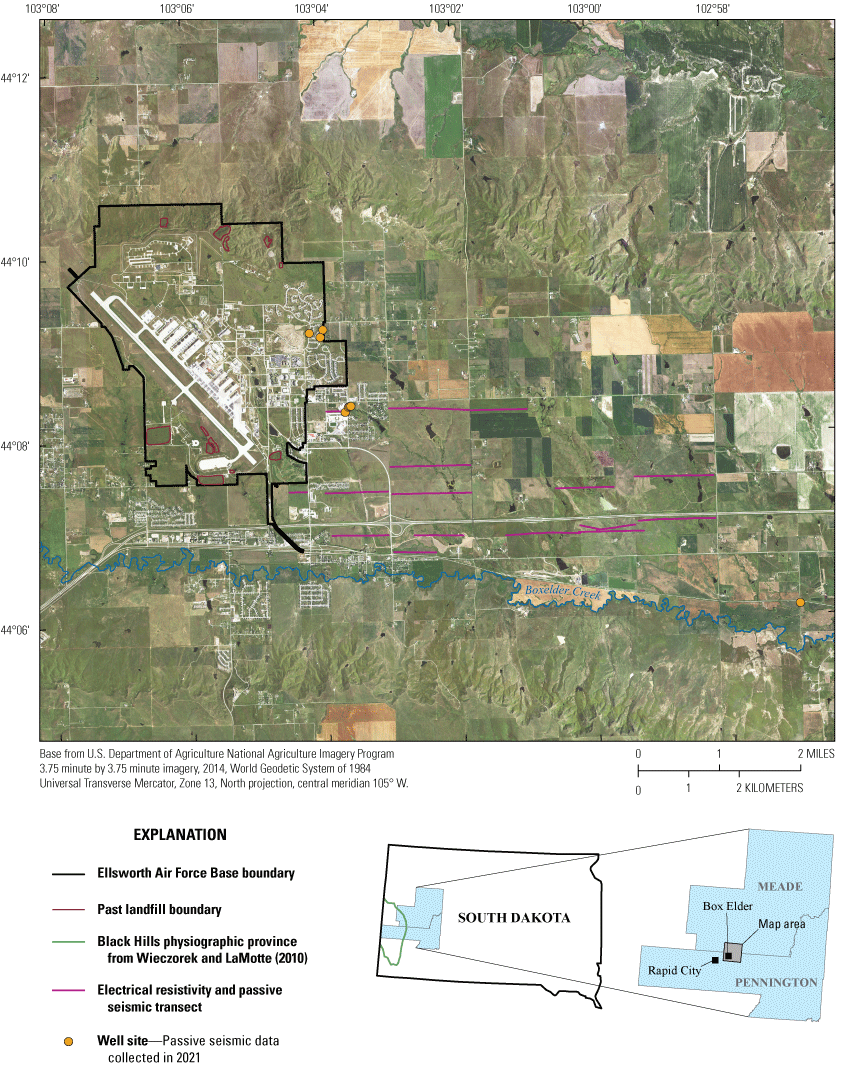
Electrical resistivity and passive seismic transects and wells where passive seismic data were collected east and southeast of Ellsworth Air Force Base, South Dakota.
The U.S. Geological Survey (USGS), in cooperation with the U.S. Air Force Civil Engineer Center, used surface-geophysical methods to delineate the top of the Cretaceous Pierre Shale (bedrock) along survey transects in selected areas east and southeast of EAFB. This study builds on previous work from Medler and Anderson (2021) that investigated the use of surface-geophysical methods for delineating the top of the bedrock within and near EAFB. Geophysical surveys provide a noninvasive means of characterizing hydrogeologic conditions to supplement available information. Two complementary geophysical methods—electrical resistivity and passive seismic—were used along 21 colocated transect surveys east and southeast of EAFB for a total of 24.7 line-kilometers (fig. 1). Electrical resistivity and passive seismic surveys were colocated for direct comparison of depth-to-bedrock estimates and to improve interpretation of the bedrock surface. Electrical resistivity data were collected along survey lines to produce two-dimensional (2D) images of subsurface resistivity, and passive seismic data were collected at a single point as soundings to provide a depth to bedrock.
Purpose and Scope
The purpose of this report is to document the results of two complementary geophysical surveys performed by the USGS from April to September 2021 east and southeast of EAFB to delineate the top of the Cretaceous Pierre Shale. Electrical resistivity and passive seismic surveys were completed along 21 colocated transects for a total of 24.7 line-kilometers. The electrical resistivity and passive seismic surveys were colocated for direct comparison and to complement the delineation of the Pierre Shale along profiles in selected areas. The purpose of delineating the Pierre Shale was to characterize unconsolidated deposits overlying the Pierre Shale east and southeast of EAFB.
Geology and Hydrogeology of Alluvial Aquifers and Pierre Shale
The geology of EAFB was described using geologic maps (Martin and others, 2004; Redden and DeWitt, 2009) and drillers logs (South Dakota Department of Agriculture and Natural Resources, 2022) that indicated that underlying the study area are the Cretaceous Pierre Shale, Quaternary terrace deposits, and Quaternary alluvial deposits (fig. 2). The study area also includes artificial fill and landfill deposits from historical and recent activities on EAFB (not shown in fig. 2). Drillers logs in the study area (South Dakota Department of Agriculture and Natural Resources, 2022) recorded landfill waste (clothing scraps, glass, and wood) at various locations at various depths in areas of past landfills (fig. 1).
The youngest geologic unit near EAFB is the unconsolidated Quaternary alluvial deposits that are near active streams and consist of mud, silt, sand, and gravel with a maximum thickness of about 10 meters (m) (fig. 2; Redden and DeWitt, 2009). Unconsolidated Quaternary terrace deposits underlie most of EAFB and are generally older and at greater elevation than alluvial deposits in the study area. The terrace deposits in the study area formed from remnants of past river systems that incised into the landscape and left behind deposits of gravel, sand, silt, and soils (McGregor and Cattermole, 1973; Redden and DeWitt, 2009). The terrace deposits can be as much as 30 m thick in the study area (Redden and DeWitt, 2009), although drillers logs indicated a mean thickness of about 10 m (South Dakota Department of Agriculture and Natural Resources, 2022). The Pierre Shale is the bedrock unit in the study area and is exposed at the surface in some areas (fig. 2). The Pierre Shale unconformably underlies Quaternary alluvial deposits and Quaternary terrace deposits with an erosional contact (Redden and DeWitt, 2009). Drillers logs from the South Dakota Department of Agriculture and Natural Resources (2022) in the study area show that the upper 4.5 to 10.0 m of the Pierre Shale can be highly weathered and fractured with oxidized iron staining.
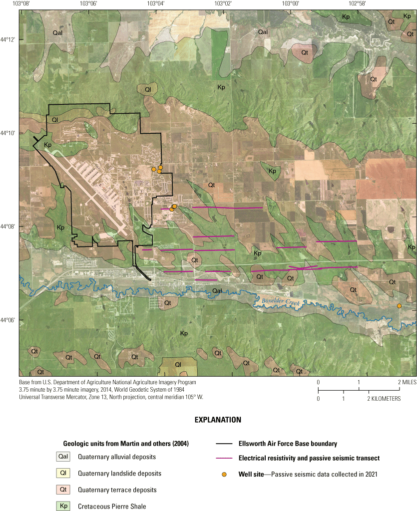
Surficial geology and electrical resistivity and passive seismic transects east and southeast of Ellsworth Air Force Base, South Dakota.
The hydrogeology of the study area was interpreted from lithologic descriptions in drillers logs (South Dakota Department of Agriculture and Natural Resources, 2022). Drillers logs indicated coarse, unconsolidated materials in Quaternary alluvial and terrace deposits overlying the Pierre Shale contain groundwater and compose the shallow unconfined aquifer at EAFB. The shallow unconfined aquifer is recharged by direct infiltration of precipitation at the land surface and by interaction with drainages and streams. Coarse materials in the shallow unconfined aquifer, such as sand and gravel, facilitate groundwater flow because of the large pore spaces and relatively high hydraulic conductivity compared to finer grained materials. Finer materials, such as clay and silt, act as barriers to groundwater flow but can store substantial amounts of water in pore spaces. Drillers logs also indicated that the upper weathered surface of the Pierre Shale contains groundwater; however, groundwater flow in the Pierre Shale likely is minimal because of its low hydraulic conductivity (Bredehoeft and others, 1983). The general direction of groundwater flow in the shallow unconfined aquifer is from northwest to southeast toward Boxelder Creek (fig. 1) but also likely approximates local surface topography in the absence of hydrogeologic structures, such as buried stream channels (Heath, 1983).
Geophysical Surveying Methods
Geophysical surveying methods used to estimate the thickness of unconsolidated Quaternary deposits and the elevation of the top of the Pierre Shale near EAFB included two-dimensional (2D) electrical resistivity tomography (ERT) and a passive seismic technique referred to as the horizontal-to-vertical spectral ratio (HVSR) method. In total, the USGS surveyed 21 transects for a total of 24.7 line-kilometers between April and September 2021 east and southeast of EAFB (fig. 1). The ERT and HVSR surveys were colocated along predetermined transects in selected areas to determine the depth to the Pierre Shale and to allow for comparison between results of both methods. Latitude, longitude, and land-surface elevation data were collected at electrical-resistivity survey electrodes using real-time kinematic (RTK) surveys. RTK surveys, hand-held global positioning systems, and elevations from light detection and ranging (lidar) survey data (City of Rapid City, 2015; U.S. Geological Survey, 2022) were used to determine the location and elevation at HVSR sites. Site information (latitude, longitude, and elevation) and geophysical survey results are available in an accompanying USGS data release to this report (Medler, 2022).
Electrical Resistivity
Electrical resistivity surveys were completed near EAFB to characterize subsurface materials and determine the depth to bedrock along transects. Electrical resistivity surveys identify horizontal and (or) vertical changes in subsurface resistivity that typically correspond to changes in lithology, chemistry of pore fluids, and (or) water content of subsurface materials (Sheets, 2002). 2D electrical resistivity surveys commonly use many electrodes equally spaced along a straight transect at the surface. The spacing of electrodes along a transect generally controls the depth of investigation and the measurement resolution. Greater electrode spacing corresponds to a greater depth of investigation but lower measurement resolution, whereas finer electrode spacing corresponds to a lesser depth of investigation but higher measurement resolution (Loke, 2000). Electrodes are connected to stainless-steel stakes spaced at a regular interval along a cable, which is connected to the resistivity meter that controls the measurements. The resistivity meter runs a pre-programmed, data-collection routine that automatically selects at least four electrodes for each measurement. Measurements consist of two current electrodes and at least two potential electrodes; electrical current is transmitted into the ground through current electrodes, and the resulting voltage is measured at the potential electrodes. Electrode groupings and the sequence of measurements are controlled by the type of array specified for the survey. Commonly used arrays include Wenner, dipole-dipole, and Schlumberger (Loke, 2000, 2004). Electrical resistivity data are then downloaded from the resistivity meter after the survey is complete and modeled using tomographic inversion software to obtain 2D cross sections of the subsurface resistivity.
Electrical resistivity data were acquired near EAFB between April and September 2021 using an 8-channel, SuperSting R8 resistivity meter (Advanced Geosciences Inc., 2022) with 56 total electrodes on 4 cable sections (14 electrodes per cable section). Electrodes along each cable were connected to stainless-steel stakes placed at evenly spaced intervals (5 m) along predetermined transects on the land surface. The land surface was sprayed with freshwater after placing electrodes to reduce electrical contact resistance with the ground before data collection. The cables were then connected to the SuperSting R8 that automatically collected resistivity data by switching between programmed combinations of current and potential electrode pairs based on the dipole-dipole array configuration. Loke (2000) and Zohdy and others (1974) provide a detailed description of the dipole-dipole array.
Some of the longer transects required the “roll-along” technique to extend the horizontal area covered by the survey. The “roll-along” technique involved moving the first cable section (electrodes 1 to 14) or the first and second electrode cable sections (electrodes 1 to 28) at the front of the survey to the end of initially placed cables with 25- or 50-percent overlap, respectively, of the previous cable layout until the desired length of transect was completed or until the surveying was completed for the day. Single-day survey lengths ranged from 345 to 975 m. Some transects were longer than what could be completed in a single day, so multiple days were required for the survey. Transects requiring 2 or more days to complete involved overlapping with the previous day’s survey to avoid data gaps in ERT results. For example, transect 1C required 3 days to complete; on the first day 555 m were completed; on the second day 555 m were completed but overlapped by 150 m with the survey completed on the first day; and the third day 555 m were completed but overlapped by 75 m with the survey completed on the second day. The overlap between multi-day surveys along the same transect ranged from 50 to 140 m.
2D ERT models were prepared for each transect using the EarthImager2D tomographic inversion software suite (https://www.agiusa.com/agi-earthimager-2d). The first step in model preparation was automatic and manual removal of noisy data in EarthImager2D. Sources of noisy data can include poor contacts between electrodes and the land surface, the presence of nearby conductors above and below land surface (metal pipes or chain-linked fences), variations in subsurface material or land-surface topography, and (or) electrical noise from internal or external factors, such as changes in current flow, battery voltage, and air temperature. The automatic data removal used seven criteria specified by EarthImager2D in the recommended settings. Additionally, noisy data were removed manually before and after inversion using an EarthImager2D utility that allows users to select specific data points that display a data misfit percentage. The second step in model preparation was to incorporate elevation information using land-surface elevation data from RTK surveys for each electrode to minimize errors from topographic changes.
The third step in model preparation was to choose the method of inversion and remove noisy data highlighted after inversion. Electrical resistivity data were modeled using least-squares smooth model inversion (Constable and others, 1987; Farquharson and Oldenburg, 1998) because the area surveyed was best approximated as a simple layered model with only two or three layers as opposed to a more complex model consisting of more than three layers with geologic structures and (or) intrusion of conductive waters, such as seawater. Smooth model inversion reduces differences between measured data and model-predicted values in a simple starting model using an iterative process, where successive iterations attempt to reduce the difference between measured data and predicted values by determining the root mean square error (rmse). The goal of smooth model inversion is to reduce the rmse until a desired error tolerance is met rather than minimize the rmse—which increases model roughness, causes artifacts, and diverges from the simple layered model (Constable and others, 1987). The maximum number of model iterations was set to eight for all ERT transects, and the accepted model was chosen as the model that best fit the site conceptual model and was closest to the convergence criteria. In some instances, noisy data missed during the first step were removed manually after the first inversion and a new inversion was completed. For all ERT transects, the model was chosen within the first five iterations and when the rmse was less than 15 percent.
Passive Seismic
Passive seismic data were collected and evaluated using the HVSR method. The HVSR method uses passive seismic data from a single, broad-band, three-component seismometer (Nakamura, 1989; Lane and others, 2007). Passive seismic methods are based on ambient seismic noise generated by wind, ocean waves, and human activities rather than artificial, “active” sources, such as an explosive charge or a hammer blow, to obtain a seismic response (Lane and others, 2008). With the HVSR method, ambient seismic noise data are analyzed by using the ratio of two averaged horizontal components (north-south and east-west) to the vertical component (up-down). For each measurement, multiple ratios are averaged to create a single curve from which the fundamental resonance frequency (f0) is determined. The f0 generally is identified as a peak on the curve with the lowest frequency and greatest amplitude. The HVSR method requires a strong acoustic impedance contrast (greater than or equal to 2) between the bedrock and overlying sediments (Lane and others, 2008), otherwise, the f0 at a site can be difficult to measure.
The f0 can be used to estimate the depth to bedrock using two techniques: 1) linear regression relating depth to bedrock (Z) and f0 or (2) estimating or using a known shear wave velocity (vs) of subsurface materials. The linear-regression technique involves collecting HVSR data at sites where the depth to bedrock is known and varies, such as a well with a documented depth to bedrock. Linear-regression results generally improve with increasing number of sites in the analysis and can be further improved by including sites covering the full range of expected depth to bedrock within a study area. The depth to bedrock (Z) and the f0 are plotted and regressed using equation 1:
whereZ
is the depth to bedrock,
f0
is the fundamental resonance frequency, and
a and b
are empirically determined constants.
After determining a and b, equation 1 can be applied to calculate depth to bedrock (Z) at sites where the f0 was determined from HVSR data. The other technique involves estimating vs by determining f0 at a site where the depth to bedrock (Z) is known using equation 2:
If the vs is estimated at many sites where the depth to bedrock is known, a mean vs can be calculated and used to determine the depth to bedrock using equation 3:
A total of 421 HVSR sites were used to supplement and confirm ERT results in determining the depth to bedrock in the study area. A TROMINO Blu three-component seismometer (https://moho.world/en/tromino/) was used to acquire passive seismic data in the study area (some transects are combined in fig. 1). Passive seismic measurements were collected every 50–100 m along the transects. At each HVSR site, the seismometer was oriented to north, leveled, and coupled directly to the ground using 3-cm long spikes to ensure the seismometer was in contact with the land surface. A weighted and inverted 5-gallon bucket was used to protect the seismometer from wind gusts during measurements. One 20-minute measurement was made at each site based on an estimated depth to bedrock from drillers logs (South Dakota Department of Agriculture and Natural Resources, 2022) of less than 16 m. In general, the depth of investigation for HVSR measurements increases with measurement time.
Two measurements were made at nine predetermined sites using two seismometers where the depth to bedrock was known from driller logs (South Dakota Department of Agriculture and Natural Resources, 2022; fig. 1). Additionally, measurements at well sites within and near EAFB from Medler and Anderson (2021) were used. Four measurements at 2 of the 9 well sites and 28 measurements at 19 well sites from Medler and Anderson (2021) produced discernable f0 peaks, which were used in equations 1 and 3 to calculate the depth to bedrock at HVSR sites where the depth to bedrock was unknown. Linear regression was used to determine empirical constants (a and b) for equation 1 and the vs used in equation 3 was determined using equation 2 with known depth to bedrock from drillers logs. The average vs was used in equation 3 to calculate the depth to bedrock at other HVSR sites where the depth to bedrock was unknown.
HVSR data were analyzed using the Grilla version 9.6.3 developed by Moho Science and Technology (https://moho.world/en/tromino/). Grilla software automatically transforms the data from the time domain to the frequency domain using a Fourier Transform and calculates the ratio between horizontal and vertical components of ambient seismic noise. A 20-second time interval with a moving standard deviation less than 1 was specified in Grilla to avoid noisy data sections. Additionally, the Konno and Ohmachi (1998) smoothing function with a constant bandwidth of 40 was specified for spectral smoothing. The result was a curve that was evaluated for amplitude and frequency of resonance peaks that corresponded to the contact between overlying sediments and bedrock (Lane and others, 2008). Sites with strong acoustic impedance contrast and little noise contamination can produce high amplitude f0 peaks; however, f0 peaks can either be absent or have low amplitude at sites with little acoustic impedance contrast or when the frequency spectrum is obscured by heavy noise contamination. Noise contamination can be caused by poor instrument coupling, heavy winds (greater than 25 or 35 kilometers per hour), or nearby human activities, such as construction or vehicle traffic.
A categorical rating system was developed to score the f0 peak at each HVSR site on a scale of 1 (very poor) to 5 (excellent) based on the peak quality and ability to be interpreted. The factors affecting each score in the categorical rating system were based on instrument coupling, the amplitude and width of its f0 peak, and noise contamination (table 1). The coupling quality was evaluated by observing the three components of ambient seismic noise in Grilla software. Sites with very poor coupling (score of 1) had large spacing between horizontal and vertical components of ambient seismic noise on amplitude spectra plots, whereas sites with excellent coupling (score of 5) had minimal spacing between all three components.
Table 1.
Description of quality scores used in the categorical rating system that determined the quality of fundamental resonance frequency (f0) peaks at horizontal-to-vertical spectral ratio sites through the coupling quality, the shape of the f0 peak (width and amplitude), and noise contamination.The amplitude and width (or shape) of f0 peaks were evaluated by comparing an f0 peak to its frequency curve at each HVSR site, as well as to f0 peaks from other HVSR sites. An f0 peak was compared to its frequency curve by determining the amplitude of the peak relative to the mean amplitude of the curve before and after the peak. The width of an f0 peak was defined by the distance between the two limbs at the half-amplitude part of the peak. The lowest amplitude and widest f0 peaks received the lowest scores (1 or 2), whereas the highest amplitude and narrowest f0 peaks received the highest scores (4 or 5; table 1). The noise contamination level was assessed by observing noise signals in the 20-minute traces for each of the three components of ambient seismic noise. Field notes that recorded wind speeds and nearby activities, such as vehicle traffic or construction, were used to verify noise signals in the three components traces and high noise sections were removed using Grilla software. Sites with low amplitude or no f0 peaks from poor acoustic impedance contrast, poor coupling, or high noise contamination were not evaluated using the rating system (table 1). Some HVSR sites that could not be evaluated were later reoccupied during relatively low wind conditions (less than 5 meters per second [m/s]) to try improving results; however, results were improved for only a small number of reoccupied sites, and the lack of improvement was attributed to low acoustic impedance contrast rather than environmental conditions (wind or human-related noise).
Two analytical methods were used to determine depth to bedrock to compare the results and select the method best suited for the dataset. For each HVSR measurement, the depth to bedrock was calculated using the f0 peak at each HVSR site in equation 3 with an average vs. Twenty-one of the 38 well sites produced clear f0 peaks, which were used in equation 2 with the known depth to bedrock from drillers logs used to calculate vs. The depth to bedrock at the 21 well sites ranged from 6.7 to 13.1 m. The average vs for the 21 well sites was 277.2 m/s with a standard deviation of 43.8 m/s. The vs of 277.2 m/s is within the typical range for site class D type materials (medium, dense sand or stiff clay) and unconsolidated deposits (Yong and others, 2016; National Earthquake Hazards Reduction Program, 2020). Equation 3 was used with the average vs to calculate the depth to bedrock at other HVSR sites where the depth to bedrock is unknown (Lane and others, 2008). The absolute difference between the true depth to bedrock from drillers logs and the depth to bedrock calculated using equation 3 with the average vs at the 21 sites where HVSR data were collected ranged from 0.0 to 4.3 m, with mean and median values of 1.2 and 1.1 m, respectively.
In addition to the two analytical methods described above, a power-law regression was fit to the same 21 sites with an equation to estimate the depth to bedrock (Z), in meters, where Z=73.42f0−1.034, with a coefficient of determination of 0.40. The absolute difference between the true depth to bedrock from drillers logs and the calculated depth to bedrock from the power-law regression equation at the 21 sites where HVSR data were collected ranged from 0.1 to 4.5 m, with mean and median values of 1.2 and 1.0 m, respectively. Additionally, calculated depth to bedrock from equation 3 with the average vs was compared to the calculated depth to bedrock using the local regression equation. The mean and median absolute difference between depth to bedrock estimates using the two methods described here were 0.12 and 0.12 m, respectively, with a standard deviation of 0.068 m. The minimum and maximum absolute differences between depth to bedrock estimates using the two methods were 0.011 and 1.052 m, respectively, with only one well site with an absolute difference greater than 0.2 m. The depth to bedrock was calculated using equation 3 with the average vs for HVSR sites along transects because the method was computationally simpler and yielded similar results to the power-law regression equation at the 21 well sites and along transects.
Real-Time Kinematic Survey
Single-base RTK surveys with Global Navigation Satellite Systems (GNSS) technology were used to measure three-dimensional positions of ERT electrodes and some HVSR sites. Single-base RTK surveys involve using a single stationary receiver (or “base station”) and a mobile unit (or “rover”) to collect spatial data at survey points. Base stations send real-time differential corrections by way of radio to a rover so the elevation of a site can be measured (Rydlund and Densmore, 2012). Before the real-time corrections are applied from the base station, the rover undergoes an initialization process that downloads information, such as the position of satellites and the time delay transmission from satellites used to calculate the rover’s position (Rydlund and Densmore, 2012). Traditionally, the base station is set up over a surveyed benchmark for comparison with established position data for quality-assurance purposes (Rydlund and Densmore, 2012); however, surveyed benchmarks are not always near to survey areas, so the base station can be set up over an unknown location. For surveys where the base station is not set up over a surveyed benchmark, the elevation and position of spatial data collected by the rover are determined as a differential from the base station (Rydlund and Densmore, 2012).
Established survey benchmarks were not used for RTK surveys in this study because they were too far from the transects in the study area for the base station and rover to maintain connection. The poor connection likely was caused by topographic obstruction, the distance between the two receivers, or a combination of both topography and distance. Instead, temporary benchmarks were established by occupying locations close to survey transects for at least 4 hours, whereas the rover was used to collect spatial data along survey transects. Static occupation files from the base stations were processed using the Online Positioning User Service (OPUS; National Geodetic Survey, 2014). The coordinates and land-surface elevation data of the electrodes and HVSR sites were adjusted based on the difference between the OPUS solution and the position data collected by the base station. Accuracy of the surveyed temporary benchmark elevations were estimated from the overall rmse calculated by the OPUS solution. The overall rmse ranged from 0.012 to 0.307 m, with an average of 0.027 m. During some surveys, the static occupation file was either not recorded or disturbed by cattle or wind. In these cases, the OPUS solution either could not be used to adjust position data from RTK surveys or had a relatively high rmse because the base station did not record position data for a sufficient amount of time (at least 4 hours). Latitude and longitude data from surveys without OPUS solutions were used in analysis and are annotated in the accompanying data release (Medler, 2022); however, the land-surface elevation from RTK surveys was not used. Instead, unadjusted latitude and longitude data from the RTK survey were used, and land-surface elevations for each electrode were estimated from lidar data (City of Rapid City, 2015).
Geophysical Survey Results
Geophysical survey results were evaluated individually and collectively to delineate the top of the Pierre Shale for 21 transects east and southeast of EAFB. 2D models from ERT inversion results were evaluated by comparing subsurface resistivity values to a surficial-geology map (Martin and others, 2004). HVSR results were individually evaluated based on a categorical rating system that assessed the quality of the f0 peak at each site by assigning a score from 1 (very poor) to 5 (excellent) (table 1). The factors affecting the quality score at each HVSR site included instrument coupling, the amplitude and width of f0 peaks, and noise contamination during the measurement. The Pierre Shale surface was delineated along each transect’s profile using ERT and HVSR results for all 21 colocated transects (sheets 1–3).
Electrical Resistivity Tomography Inversion Results
The ERT inversion results showed a range of subsurface resistivity values that varied among transects. The spatial distribution of resistivity values for ERT transects was investigated using a surficial-geology map (Martin and others, 2004). ERT transects mostly intersected Cretaceous Pierre Shale and Quaternary terrace deposits but also intersected Quaternary alluvial deposits (sheets 1–3). ERT inversion results of some transects showed that resistivity values of Quaternary terrace deposits generally decreased with decreasing land-surface elevation from north to south and (or) from west to east away from the Black Hills (about the same extent as the Black Hills physiographic province in fig. 1) along transects. For example, resistivity values of Quaternary terrace deposits along the northernmost (transects 1C and 1D) and westernmost transects (transects 3A and 4A) generally were greater than resistivity values of transects further south and east (sheets 1–3). Additionally, resistivity values decreased near streams and (or) near surface contacts with other geologic units, such as the Pierre Shale. For example, resistivity values along transect 1C decreased with proximity to exposures of the Pierre Shale and (or) stream crossings from about 450 to 800 m and from 1,200 to 1,280 m along the transect (sheet 1). The directional decrease in resistivity values from north to south and west to east, as well as toward streams and other geologic units, was interpreted as a decrease in thickness or the absence of Quaternary terrace deposits.
A surficial-geology map from Martin and others (2004) showed that 17 of the 21 ERT transects intersected the Pierre Shale. Transects intersecting the Pierre Shale included 1C, 2, 3B, 3D, 3E, 3F, 4A, 4B, 4D, 4E, 4F alternate 1, 4F alternate 2, 4FD3, 4FD4, 4FD5, 4G, and 4H (sheets 1–3). ERT inversion results from the 17 ERT transects showed resistivity values less than about 30 ohm-meters (ohm-m) at or near the surface where the Pierre Shale was intersected. For example, the resistivity values along transects 4G and 4H are less than 30 ohm-m throughout most of the ERT profile (sheet 3). The expected range of resistivity values for the Pierre Shale was determined to be between 10 and 30 ohm-m by Medler and Anderson (2021). The relatively low resistivity values of the Pierre Shale can be attributed to its mineralogic composition (Loke, 2004); geochemistry data from the Pierre Shale indicate that shale is rich in conductive clay minerals (Schultz and others, 1980). Therefore, the electrical conductivity (the inverse of electrical resistivity) of the clay minerals is higher than the silica-rich overlying unconsolidated deposits. ERT inversion results showed that resistivity values of the Pierre Shale decrease with increasing depth—indicating the quantity of conductive materials may be increasing with depth. The Pierre Shale at or near the surface displayed higher resistivity values than expected likely because of a greater degree of weathering, which reduces the quantity of conductive clay minerals and increases the resistivity.
Many profiles in sheets 1–3 showed resistivity values greater than 30 ohm-m within 1 to 3 m of land surface where a geologic map indicated the Pierre Shale was intersected. For example, the eastern part of transect 2 from about 1,250 to 1,560 m along the profile showed resistivity values greater than 30 ohm-m where the geologic map indicated the Pierre Shale was exposed at land surface (sheet 2). The absence of low resistivity values from 1,250 to 1,560 m along transect 2 indicated that the Pierre Shale does not crop out as shown in the geologic map (Martin and others, 2004). It should be noted that the geologic map used for comparison with ERT inversion results (Martin and others, 2004) was prepared at a 1:500,000 scale for the entire State of South Dakota and may not meet accuracy requirements for spatial comparisons in this study. A geologic map from Redden and DeWitt (2009) was prepared at a smaller scale (1:250,000) but does not cover the full extent of ERT transects in this study, and, therefore, could not be used for comparison. However, where both geologic maps overlap, the Pierre Shale crops out in and along the margins of stream valleys. The ERT inversion results showed lower resistivity values consistent with the Pierre Shale near streams, so it is likely the Pierre Shale crops out along streams as indicated by Martin and others (2004) and Redden and DeWitt (2009).
Horizontal-to-Vertical Spectral Ratio Results
The HVSR results were evaluated using a categorical rating system to assess the quality of f0 peaks. The rating system scored each HVSR site on a scale of 1 (very poor) to 5 (excellent) (table 1) based on instrument coupling, the amplitude and width of its f0 peak, and noise contamination. The HVSR sites with high scores generally had good coupling, high amplitude, narrow f0 peaks, and (or) low noise contamination, whereas HVSR sites with low scores had relatively poor coupling, low amplitude, broad f0 peaks, and (or) high noise contamination. The distribution of quality scores for f0 peaks at all HVSR sites is shown in figure 3. An additional category shows the measurements with no observable f0 peak that could not be scored using the categorical rating system (table 1). HVSR sites with quality scores 1 and 2 accounted for about 35 percent of all sites scored; HVSR sites with quality scores 3–5 accounted for about 21 percent of all sites scored; and HVSR sites with no observable f0 peak accounted for 44 percent of all sites scored.
The distribution of quality scores for HVSR sites was attributed to varying environmental conditions, such as changes in wind speed or vehicle traffic, and spatial changes in acoustic impedance contrast between the Pierre Shale and overlying surficial deposits throughout the study area. Field notes recorded during data collection were inspected for each HVSR site to examine the effect of environmental conditions on f0 peaks. Discernable f0 peaks were observed during time periods of favorable and unfavorable environmental conditions. In some instances, HVSR data collected during periods of favorable environmental conditions produced indiscernible f0 peaks that received no quality score. In these instances, the indiscernible f0 peak was attributed to the acoustic impedance contrast between the Pierre Shale and overlying surficial deposits. The acoustic impedance contrast may have varied because of several factors, including (1) differences in the degree of weathering of the Pierre Shale, (2) lithological similarities or differences between the Pierre Shale and overlying surficial deposits, or (3) changes in the structure of the bedrock surface. The quality codes also were investigated for spatial patterns, but no observable patterns were apparent.
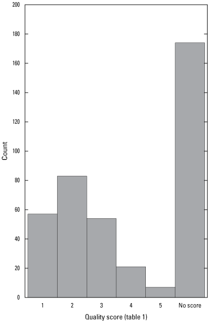
Distribution of quality scores from 1 to 5 (very poor to excellent) and no score for fundamental resonance frequency (f0) peaks from horizontal-to-vertical spectral ratio sites and the number of horizontal-to-vertical spectral ratio sites not scored.
Depth to bedrock estimates at HVSR sites along transects were converted to elevations by subtracting the estimated depth to bedrock from the land-surface elevation at each HVSR site. The calculated elevation of the top of Pierre Shale from HVSR results are shown in sheets 1–3. Five sources of error possibly affecting the bedrock-elevation estimates at HVSR sites were identified, including (1) inaccuracies of land-surface elevations of HVSR sites, (2) errors in reported depth to Pierre Shale in drillers logs, (3) the range of depths to Pierre Shale and f0 values from wells used in calculating the average vs, (4) poor f0 peaks that were difficult to discern, and (or) (5) selection of f0 peaks representing contacts other than unconsolidated deposits and Pierre Shale. The following paragraphs will describe each source of error and the steps taken to avoid or minimize any inaccuracies.
Depth to bedrock estimates at HVSR sites along transects were converted to elevations by subtracting the land-surface elevation of the HVSR site by the calculated depth to bedrock. If the land-surface elevation—obtained from either RTK surveys or lidar data—was inaccurate, then the bedrock elevation along survey transects in sheet 1–3 also would be inaccurate. Most land-surface elevation data were obtained from RTK surveys; however, land-surface elevation discrepancies between RTK surveys and lidar data at HVSR sites could be present. If possible, the land-surface elevation of HVSR sites obtained from lidar data were compared to the land- surface elevation of the nearest ERT electrode to ensure that the elevations were similar. The absolute minimum and maximum land-surface elevation differences between HVSR sites and the nearest ERT electrodes were 0.0 and 3.7 m, respectively, with mean and median absolute differences of 0.20 and 0.06 m, respectively. This difference was considered to have minimal effect on the accuracy and precision of the delineations shown on sheets 1–3.
The depth to Pierre Shale obtained from drillers logs for wells used in calculating depth to bedrock also was a potential source of error in the analysis. If the depths to Pierre Shale were reported incorrectly at wells where HVSR data were collected, then the depth to bedrock estimates calculated using the average vs in equation 3 could be affected. The vs was determined at each well site using equation 2, which requires a known depth to bedrock. Therefore, if the true depth to bedrock was different than that reported in drillers logs, the vs would change. Drillers logs for each well from the South Dakota Department of Agriculture and Natural Resources (2022) were thoroughly inspected to avoid incorrect depths to Pierre Shale; however, the Pierre Shale may have been misidentified at some well sites, causing the reported depth to Pierre Shale to be incorrect. Drillers logs at some wells reported clay layers directly overlying the Pierre Shale that were difficult to distinguish from the Pierre Shale and may have been reworked or weathered shale with similar properties as overlying unconsolidated deposits. Wells where the Pierre Shale was indistinguishable from overlying materials were removed from analysis to avoid erroneous vs estimates.
Calculation of the average vs used in equation 3 to estimate depth to bedrock at HVSR sites along transects could be another source of error. The average vs was calculated for each well using the f0 value and the corresponding known depth to bedrock from a drillers logs in equation 2. HVSR sites along transects with a f0 value or a true depth to Pierre Shale outside of the f0 and depth ranges included in determination of the average vs may not be accurately reproduced using equation 3. The f0 values and depth to Pierre Shale ranged from 5.63 to 9.09 hertz and from 6.7 to 13.1 m, respectively, for the wells included in vs analysis. About 53 percent of discernable f0 peaks at HVSR sites were within the range of the f0 values for wells included in vs analysis. About 70 percent of all estimated depths to Pierre Shale at HVSR sites along transects were within the range of depth to the Pierre Shale for wells included in the analysis. The estimated depth to Pierre Shale at these HVSR sites could be more accurate if more data were included from larger ranges of f0 values and depth to the Pierre Shale. Therefore, the average vs used in equation 3 may have overestimated or underestimated the depth to the Pierre Shale at the 47 and 30 percent of HVSR sites along transects outside the f0 and depth to Pierre Shale ranges, respectively, at wells included in the analysis.
The depth to Pierre Shale estimates calculated with equation 3 were compared to depth to the Pierre Shale calculated using the local regression equation to determine if the two methods applied in this study provided similar results. The local regression equation (Z=73.42f0−1.034) was used to estimate the depth to Pierre Shale for HVSR sites along transects based on the same well data used to calculate the average vs used in equation 3. The difference in estimated depth to Pierre Shale between equation 3 and the local regression equation was calculated by subtracting the depth estimated from equation 3 by the depth estimated with the local regression equation. The mean and median differences in depth to the Pierre Shale were about 0.11 and 0.12 m, respectively, and the minimum and maximum differences were about −0.15 and 1.05 m, respectively. Additionally, about 98 percent of the differences were above zero, indicating that the depth to the Pierre Shale calculated using equation 3 were typically greater than the depth to the Pierre Shale calculated using the local regression equation. Equation 3 with the average vs underestimated and overestimated the depth to the Pierre Shale for HVSR sites with the lowest and highest f0 values, respectively, when compared to the power-law regression equation, but performed well for most sites. The absolute difference in depth to bedrock between the two methods was less than 0.2 m for all but one the HVSR sites along transects.
Another possibility for a source of error for depth to the Pierre Shale estimates was the erroneous selection of f0 peaks from data affected by poor coupling, noise contamination, or poor acoustic impedance. Poor coupling and noise contamination were observed at various HVSR sites along transects and at some wells. HVSR sites with poor coupling and (or) noise contamination often required additional filtering, which sometimes did not produce an observable f0 peak. Weak acoustic impedance contrast between clay-rich unconsolidated deposits and the Pierre Shale also likely contributed to flat and difficult to discern f0 peaks (ratings 1–2). Erroneous selection of f0 peaks affects calculations of the average vs used in equation 3 and of the estimated depth to bedrock at HVSR sites along transects. Selecting an f0 peak other than true f0 peak for each well site also could change the calculated vs from equation 2 at each well site, which could change the average vs. Erroneous selection of f0 peaks at HVSR sites along transects could affect the estimated depth to the Pierre Shale using equation 3 because the f0 peak value is the only non-constant variable in the equation. Some HVSR data that displayed low amplitude and broad f0 peaks (ratings of 1–2) were included in calculations of the average vs and depth to the Pierre Shale at HVSR sites along transects. Sixteen of the 28 HVSR sites used in calculation of the average vs received a quality score of 1 or 2 and were included so that range of f0 peak values and range of depth to bedrock used to calculate the average vs represented f0 and vs values expected at HVSR sites along transects with unknown depth to bedrock.
Geologic contacts other than those between unconsolidated deposits and the Pierre Shale also may have affected depth estimates to the shale. The f0 peaks at HVSR sites that underestimated the depth to the Pierre Shale may have correlated with a contact between sand-and-gravel-rich and clay-rich zones, rather than the contact between unconsolidated deposits and the Pierre Shale. The f0 peaks that overestimated the depth to Pierre Shale may have correlated with the transitional contact between weathered and competent Pierre. Drillers logs from wells penetrating the Pierre Shale west of the survey transects showed a transition zone from weathered to competent shale with thicknesses up to 10.0 m (South Dakota Department of Agriculture and Natural Resources, 2022). Estimated depth to Pierre Shale at HVSR sites along transects could not be compared to known depth to bedrock at nearby wells because wells with lithologic information from drillers logs were not available near survey transects. Instead, the depth to bedrock at HVSR sites was evaluated by comparing depth estimates to ERT inversion results, which is discussed in the following section.
Delineation of the Pierre Shale
The ERT and HVSR results were used to delineate the top of the Pierre Shale along 21 transects in selected areas east and southeast of EAFB. The depth to the Pierre Shale along transects ranged from 0.0 m (transects 1C, 3B, 3E, 3F) to 19.8 m (transect 1C); mean and median depths were about 6.1 and 5.6 m, respectively. The summary statistics for the depth to the Pierre Shale for transects in sheets 1–3 are shown in table 2. The mean depth to the Pierre Shale exceeded 7.5 m along transects 1C, 3A, 4A, 4D, 4E, and 4FD3. Greater mean depth to the Pierre Shale was expected along the westernmost and northernmost transects because drillers logs from nearby wells indicated Quaternary terrace deposits generally thin and disappear to the south and east (South Dakota Department of Agriculture and Natural Resources, 2022).
Table 2.
Summary statistics of the depth to the Pierre Shale for each of the geophysical transects shown in sheets 1–3.The mean depth to the Pierre Shale was less than 5.0 m along transects 3B, 3E, 4B, 4F alternate 2 (sheets 1–3). Thickness of Quaternary terrace deposits was expected to be least along the southernmost transects where the Pierre Shale crops out more frequently, and drillers logs from nearby wells indicate decreased thickness of Quaternary terrace deposits (South Dakota Department of Agriculture and Natural Resources, 2022). Additionally, the southernmost transects that intersected the Pierre Shale at the land surface had relatively low subsurface resistivity values at depths less than 5.0 m below the land surface, minimal resistivity variation, or both. The elevation of the Pierre Shale generally increased with land-surface elevation along individual transects and from south to north and east to west; however, some transects displayed the Pierre Shale in topographically high and low elevation areas along transects that sometimes did not correlate with land-surface topography (sheets 1–3).
The delineated elevation surfaces of the top of Pierre Shale in sheets 1–3 were based on transitions from high to low resistivity at about 30 ohm-m. ERT results were preferred over HVSR results for delineation because the 2D models provided a more discernable and horizontally complete image of the Pierre Shale along transects; however, HVSR results were useful for filling ERT data gaps and verifying the Pierre Shale surface interpreted from ERT profiles. Wells with drillers logs containing lithologic information could not be used to constrain the delineation of the Pierre Shale along ERT and HVSR transects because the wells were at least 450 m from the transects. The depth to the Pierre Shale likely was underestimated in areas where unconsolidated deposits are lithologically similar to the Pierre Shale. In other areas, the depth to the Pierre Shale likely was overestimated where the weathered upper part of the Pierre Shale could not be distinguished from unconsolidated deposits because of minimal differences in electrical properties and low acoustic impedance contrast at HVSR sites. The overestimated depth to the Pierre Shale at some HVSR sites likely was from an f0 peak corresponding to the transition from weathered to unweathered Pierre Shale rather than unconsolidated deposits to Pierre Shale.
Summary
The U.S. Geological Survey (USGS), in cooperation with the U.S. Air Force Civil Engineer Center, used surface-geophysical methods to delineate the top of Cretaceous Pierre Shale (bedrock) along survey transects in selected areas east and southeast of Ellsworth Air Force Base (EAFB). Two complementary geophysical methods—electrical resistivity and passive seismic—were used along 21 colocated transect surveys east and southeast of EAFB for a total of 24.7 line-kilometers. Electrical resistivity and passive seismic surveys were colocated for direct comparison and to improve interpretation of the bedrock surface. Electrical resistivity data were collected in a line-fashion to produce two-dimensional images of subsurface resistivity, whereas passive seismic data were collected as soundings to provide a depth to bedrock at a single point. Two-dimensional electrical resistivity tomography (ERT) models were prepared for each transect using tomographic inversion software. Passive seismic data were collected and evaluated using the horizontal-to-vertical spectral ratio (HVSR) method where an equation using the average shear wave velocity was calculated to determine the depth to bedrock.
Geophysical survey results were evaluated individually and collectively to delineate the top of the Pierre Shale for 21 transects east and southeast of EAFB. The spatial distribution of resistivity values for ERT transects was investigated using a surficial-geology map. ERT transects mostly intersected Cretaceous Pierre Shale and Quaternary terrace deposits but also intersected Quaternary alluvial deposits. ERT inversion results of some transects showed that resistivity values of Quaternary terrace deposits generally decreased with decreasing land-surface elevation from north to south and (or) from west to east away from the Black Hills along transects. The ERT inversion results of some transects indicated that resistivity values of Quaternary terrace deposits generally decreased toward streams and surface contacts with other geologic units, such as the Pierre Shale. A surficial-geology map showed that 17 of the 21 ERT transects intersected the Pierre Shale. Many profiles showed resistivity values greater than 30 ohm-m within 5–10 meters (m) of the land surface where a geologic map indicated the Pierre Shale was intersected. ERT inversion results showed lower resistivity values consistent with the Pierre Shale near streams, so it is likely the Pierre Shale crops out along streams as indicated in previous investigations.
The HVSR results were evaluated using a categorical rating system to assess the quality of fundamental resonance frequency (f0) peaks. The rating system scored each HVSR site on a scale from 1 (very poor) to 5 (excellent) based on the instrument coupling, the amplitude and width of its f0 peak, and noise contamination. HVSR sites with quality scores 1 and 2 accounted for about 35 percent of all sites scored; HVSR sites with quality scores 3–5 accounted for about 21 percent of all sites scored; and HVSR sites with no observable f0 peak accounted for 44 percent of all sites scored. The distribution of quality scores for HVSR sites was attributed to varying environmental conditions, such as changes in wind speed or vehicle traffic, and spatial changes in acoustic impedance contrast between the Pierre Shale and overlying surficial deposits throughout the study area. The acoustic impedance contrast may have varied because of multiple factors, including (1) differences in the degree of weathering of the Pierre Shale, (2) lithological similarities or differences between the Pierre Shale and overlying surficial deposits, or (3) changes in the structure of the bedrock surface. The quality codes also were investigated for spatial patterns, but no observable patterns were apparent.
The ERT and HVSR results were used to delineate the top of the Pierre Shale along 21 transects in selected areas east and southeast of EAFB. The depth to the Pierre Shale along transects ranged from 0.0 (transects 1C, 3B, 3E, 3F) to 19.8 m (transect 1C); mean and median depths were about 6.1 and 5.6 m, respectively. The greatest mean depth to the Pierre Shale was observed (in descending order) along transects 1C, 3A, 4A, 4D, 4E, 4FD3, where the mean depth exceeded 7.5 m. The greatest mean depth to the Pierre Shale was expected along the westernmost and northernmost transects because drillers logs from nearby wells indicated Quaternary terrace deposits generally thin and disappear to the south and east.
The mean depth to Pierre Shale was less than 5.0 m along transects 3B, 4B, 4F alternate 2, and 3E. Thickness of Quaternary terrace deposits was expected to be lesser along the southernmost transects where the Pierre Shale crops out more frequently, and drillers logs from nearby wells show decreased thickness of Quaternary terrace deposits. The elevation of the Pierre Shale generally increased with land-surface elevation along individual transects and from south to north and east to west; however, some transects displayed the Pierre Shale in topographically high and low elevation areas along transects that sometimes did not correlate with land-surface topography.
The delineated elevation surfaces of the top of Pierre Shale were based on transitions from high to low resistivity at about 30 ohm-meters. ERT results were preferred over HVSR results for delineation because the two-dimensional (2D) models provided a more discernable and horizontally complete image of the Pierre Shale along transects; however, HVSR results were useful for filling ERT data gaps and verifying the Pierre Shale surface interpreted from ERT profiles. Wells with drillers logs containing lithologic information could not be used to constrain the delineation of the Pierre Shale along ERT and HVSR transects because the wells were at least 450 m from transects. The depth to the Pierre Shale along transects likely was underestimated from unconsolidated deposits being lithologically similar to the Pierre Shale or overestimated from the weathered upper part of the Pierre Shale, resulting in minimal differences in electrical properties and a low acoustic impedance contrast for HVSR. The overestimated depth to the Pierre Shale at some HVSR sites likely was from an f0 peak corresponding to the transition from weathered to unweathered Pierre Shale rather than unconsolidated deposits to Pierre Shale.
References Cited
Advanced Geosciences Inc, 2022, High-speed 2D/3D resistivity/IP/SP imaging system package—56 electrodes: Advanced Geosciences Inc. web page, accessed January 2022 at https://www.agiusa.com/high-speed-2d3d-resistivityipsp-imaging-system-package-56-electrodes.
Bredehoeft, J.D., Neuzil, C.E., and Milly, P.C.D., 1983, Regional flow in the Dakota aquifer—A study of the role of confining layers: U.S. Geological Survey Water-Supply Paper 2237, 45 p., accessed November 2022 at https://doi.org/10.3133/wsp2237.
City of Rapid City, 2015, Rapid City LiDAR Spring 2015: Rapid City Graphic Information System Division, accessed August 2022 at https://www.rcgov.org/departments/public-works/geographic-information-system/gis-data-216.html.
Constable, S.C., Parker, R.L., and Constable, C.G., 1987, Occam’s inversion—A practical algorithm for generating smooth models from electromagnetic sounding data: Geophysics, v. 52, no. 3, p. 289–300, accessed January 2022 at https://doi.org/10.1190/1.1442303.
Farquharson, C.G., and Oldenburg, D.W., 1998, Non-linear inversion using general measures of data misfit and model structure: Geophysical Journal International, v. 134, no. 1, p. 213–227, accessed January 2022 at https://doi.org/10.1046/j.1365-246x.1998.00555.x.
Heath, R.C., 1983, Basic ground-water hydrology: U.S. Geological Survey Water-Supply Paper 2220, 86 p., accessed November 2022 at https://doi.org/10.3133/wsp2220.
Konno, K., and Ohmachi, T., 1998, Ground motion characteristics estimated from spectral ratio between horizontal and vertical components of microtremor: Bulletin of the Seismological Society of America, v. 88, no. 1, p. 228–241, accessed November 2022 at https://doi.org/10.1785/BSSA0880010228.
Lane, J.W., Jr., White, E.A., Steele, G.V., and Cannia, J.C., 2008, Estimation of bedrock depth using the horizontal-to-vertical (H/V) ambient-noise seismic method, in Symposium on the Application of Geophysics to Engineering and Environmental Problems, April 6–10, 2008, Philadelphia, Pa., Proceedings: Denver, Colo., Environmental and Engineering Geophysical Society, 13 p., accessed January 2022 at https://water.usgs.gov/ogw/bgas/publications/SAGEEP2008-Lane_HV/.
Loke, M.H., 2000, Electrical imaging surveys for environmental and engineering studies—A practical guide to 2-D and 3-D surveys: Geometrics, Inc., 57 p., accessed November 2022 at https://pages.mtu.edu/~ctyoung/LOKENOTE.PDF.
Loke, M.H., 2004, Tutorial—2-D and 3-D electrical imaging surveys: M.H. Loke, 157 p., accessed January 2022 at https://sites.ualberta.ca/~unsworth/UA-classes/223/loke_course_notes.pdf.
Martin, J.E., Sawyer, J.F., Fahrenbach, M.D., Tomhave, D.W., and Schulz, L.D., 2004, Geologic map of South Dakota: South Dakota Geological Survey General Map G–10, accessed January 2022 at http://www.sdgs.usd.edu/pubs/pdf/G-10.pdf.
McGregor, E.E., and Cattermole, J.M., 1973, Geologic map of the Rapid City NW quadrangle, Meade and Pennington Counties, South Dakota: U.S. Geological Survey Geologic Quadrangle 1093, accessed November 2022 at https://doi.org/10.3133/gq1093.
Medler, C.J., and Anderson, T.M., 2021, Delineating the Pierre Shale from geophysical surveys within and near Ellsworth Air Force Base, South Dakota, 2019: U.S. Geological Survey Scientific Investigations Map 3474, 3 sheets, 16 p. pamphlet, accessed August 2022 at https://doi.org/10.3133/sim3474.
Medler, C.J., 2022, Electrical resistivity tomography (ERT) and horizontal-to-vertical spectral ratio (HVSR) data collected East and Southeast of Ellsworth Air Force Base, South Dakota, in 2021: U.S. Geological Survey data release, https://doi.org/10.5066/P9X57BS0.
National Earthquake Hazards Reduction Program, 2020, NEHRP recommended seismic provisions for new buildings and other structures: Washington D.C., Building Safety Council, FEMA P–2082–1, v. 1, part 1 provisions, part 2 commentary, 593 p., accessed January 2022 at https://www.fema.gov/sites/default/files/2020-10/fema_2020-nehrp-provisions_part-1-and-part-2.pdf.
National Geodetic Survey, 2014, National Geodetic Survey Data Explorer—Data sheet for permanent identifier PU2524: National Oceanic and Atmospheric Administration digital data, accessed January 2022 at https://www.ngs.noaa.gov/.
Redden, J.A., and DeWitt, E., 2009, Maps showing geology, structure, and geophysics of the central Black Hills, South Dakota: U.S. Geological Survey Scientific Investigations Map 2777, scale 1:100,000, accessed January 2022 at https://ngmdb.usgs.gov/ngm-bin/pdp/zui_viewer.pl?id=16864.
Rydlund, P.H., Jr., and Densmore, B.K., 2012, Methods of practice and guidelines for using survey-grade global navigation satellite systems (GNSS) to establish vertical datum in the United States Geological Survey: U.S. Geological Survey Techniques and Methods, book 11, chap. D1, 102 p., accessed January 2022 at https://doi.org/10.3133/tm11D1.
Schultz, L.G., Tourtelot, H.A., Gill, J.R., and Boerngen, J.G., 1980, Composition and properties of the Pierre Shale and equivalent rocks, northern Great Plains region: U.S. Geological Survey Professional Paper 1064–B, 114 p., 1 plate, accessed August 2022 at https://doi.org/10.3133/pp1064B.
Sheets, R.A., 2002, Use of electrical resistivity to detect underground mine voids in Ohio: U.S. Geological Survey Water-Resources Investigations Report 2002–4041, 33 p., accessed November 2022 at https://doi.org/10.3133/wri024041.
South Dakota Department of Agriculture and Natural Resources, 2022, Water well completion reports: South Dakota Department of Agriculture and Natural Resources database, accessed January 2022 at https://apps.sd.gov/nr68welllogs/.
U.S. Environmental Protection Agency, 2022a, Superfund site—Ellsworth Air Force Base, SD: U.S. Environmental Protection Agency, accessed January 2022 at https://cumulis.epa.gov/supercpad/cursites/csitinfo.cfm?id=0800585.
U.S. Environmental Protection Agency, 2022b, Superfund—National Priorities List (NPL): U.S. Environmental Protection Agency, accessed August 2022 at https://www.epa.gov/superfund/superfund-national-priorities-list-npl.
U.S. Geological Survey, 2018, USGS National Hydrography Dataset Plus High Resolution (NHDPlus HR) for 4-digit Hydrologic Unit 1012 (published 20180503): U.S. Geological Survey, accessed April 2022 at https://www.usgs.gov/national-hydrography/access-national-hydrography-products.
U.S. Geological Survey, 2022, What is Lidar data and where can I download it?: U.S. Geological Survey, accessed August 2022 at https://www.usgs.gov/faqs/what-lidar-data-and-where-can-i-download-it.
Wieczorek, M., and LaMotte, A.E., 2010, Attributes for MRB_E2RF1 catchments by major river basins in the conterminous United States—Physiographic provinces: U.S. Geological Survey Data Series 491–18, accessed April 2022 at https://doi.org/10.3133/dds49118.
Yong, A., Thompson, E.M., Wald, D., Knudsen, K.L., Odum, J.K., Stephenson, W.J., and Haefner, S., 2016, Compilation of VS30 data for the United States: U.S. Geological Survey Data Series 978, 8 p., accessed November 2022 at https://doi.org/10.3133/ds978.
Zohdy, A.A.R., Eaton, G.P., and Mabey, D.R., 1974, Application of surface geophysics to groundwater investigations: U.S. Geological Survey Techniques of Water-Resources Investigations, book 2, chap. D1, 116 p., accessed January 2022 at https://doi.org/10.3133/twri02D1.
Datum
Vertical coordinate information is referenced to the North American Vertical Datum of 1988 (NAVD 88)
Horizontal coordinate information is referenced to the North American Datum of 1983 (NAD 83)
For more information about this publication, contact:
Director, USGS Dakota Water Science Center
821 East Interstate Avenue, Bismarck, ND 58503
1608 Mountain View Road, Rapid City, SD 57702
605–394–3200
For additional information, visit: https://www.usgs.gov/centers/dakotawater
Publishing support provided by the
Rolla Publishing Service Center
Disclaimers
Any use of trade, firm, or product names is for descriptive purposes only and does not imply endorsement by the U.S. Government.
Although this information product, for the most part, is in the public domain, it also may contain copyrighted materials as noted in the text. Permission to reproduce copyrighted items must be secured from the copyright owner.
Suggested Citation
Medler, C.J., 2022, Delineating the Pierre Shale from geophysical surveys east and southeast of Ellsworth Air Force Base, South Dakota, 2021: U.S. Geological Survey Scientific Investigations Map 3497, 3 sheets, 15-p. pamphlet, https://doi.org/10.3133/sim3497.
ISSN: 2329-132X (online)
Study Area
| Publication type | Report |
|---|---|
| Publication Subtype | USGS Numbered Series |
| Title | Delineating the Pierre Shale from geophysical surveys east and southeast of Ellsworth Air Force Base, South Dakota, 2021 |
| Series title | Scientific Investigations Map |
| Series number | 3497 |
| DOI | 10.3133/sim3497 |
| Publication Date | December 19, 2022 |
| Year Published | 2022 |
| Language | English |
| Publisher | U.S. Geological Survey |
| Publisher location | Reston, VA |
| Contributing office(s) | Dakota Water Science Center |
| Description | Report: vi, 15 p.; 3 Sheets: 64.00 × 53.33 inches or smaller; Data Release |
| Country | United States |
| State | South Dakota |
| Online Only (Y/N) | Y |
| Additional Online Files (Y/N) | Y |