

Potentiometric Surface Map of the Southern High Plains Aquifer in the Cannon Air Force Base Area, Curry County, New Mexico, 2020
Links
- Document: SIM 3504 pamphlet (1.42 MB pdf) , HTML , XML
- Plate: SIM 3504 sheet (20.5 MB pdf)
- Dataset: USGS Dataset—USGS Water Data for the Nation
- NGMDB Index Page: National Geologic Map Database Index Page (html)
- Download citation as: RIS | Dublin Core
Acknowledgments
The authors would like to thank the U.S. Air Force Civil Engineer Center for funding assistance as well as the environmental department on Cannon Air Force Base in Clovis, New Mexico. The authors deeply appreciate the cooperation of the residents near Cannon Air Force Base for allowing this survey to take place. The authors are very grateful to U.S. Geological Survey (USGS) employees Fredrick Gebhardt, Erik Storms, Hal Nelson, Elaiya Jurney, Natalia Montero, and Cooper Bailey for the newly collected USGS data that are published in this report. The authors would like to thank USGS employees Stuart Norton, Lauren Henson, and Erin Gray for their guidance and assistance in the completion of this project. The authors would also like to thank USGS employees Jeff Pepin and Andre Ritchie for their assistance with R-Studio.
Abstract
Declining water levels and the potential impact on water resources on and around Cannon Air Force Base (AFB), New Mexico, has necessitated an up-to-date review of the potentiometric surface to evaluate the availability of water resources for future use. Analysis of groundwater-flow directions and hydraulic gradients can provide an understanding of depletion by heavy groundwater pumping and recharge through playa lakes, as well as the relationship between the groundwater levels and underlying geology. The objectives of this study, conducted by the U.S. Geological Survey in cooperation with the U.S. Air Force Civil Engineer Center, are to assist Cannon AFB in understanding and interpreting current and local hydrologic conditions and to evaluate groundwater-level change from 2015 to 2020 using new and historical data. A groundwater potentiometric surface contour map was constructed to better understand the Southern High Plains aquifer around Cannon AFB and to show the altitude of the water-table surface and groundwater-flow patterns. Four hydrographs were created from periodic measurements of groundwater levels in wells on and around Cannon AFB to provide information about historical groundwater-level changes and visualize trends from the water-level records. The long-term trend present in all four hydrographs is a steady decline in groundwater levels, with some areas declining faster than others. The groundwater-level change map presented in this study provides a visual representation of the change in groundwater level from the winter 2015 to winter 2020 measuring events. Results show that among corresponding wells measured in 2015 and 2020, 50.7 percent indicated a decline in water levels, 29.9 percent indicated neutral water levels, and 19.4 percent indicated a rise in water levels. The region to the north of the groundwater trough on Cannon AFB contained most of the groundwater-level rises, whereas the regions located near the trough and just west of Clovis, N. Mex., contained most of the declines. These results suggest that continued monitoring of declining groundwater levels in the area would provide valuable decision-support information for assessing the sustainability of this water resource.
Introduction
Cannon Air Force Base (Cannon AFB) is in the Great Plains physiographic province of east-central New Mexico, in Curry County about 8 miles west of Clovis (fig. 1) (Miller, 2000). The area surrounding the base is primarily used for agriculture that includes irrigated croplands and dairies. The Southern High Plains aquifer is the principal source of water for Cannon AFB, the nearby town of Clovis, and for the local agriculture and dairies. Within this area, the unconfined Southern High Plains aquifer consists of three subsurface geologic formations: the top of the Triassic Dockum Group (Chinle Formation), the Tertiary Ogallala Formation, and the Quaternary Blackwater Draw Formation (Langman and others, 2006). Declining groundwater levels and the potential impact on water resources has necessitated an up-to-date review of the potentiometric surface to evaluate the availability of water resources for future use (Langman and others, 2006). A groundwater-level survey with associated hydrographs and maps of the potentiometric surface (the surface representing the hydraulic head, the altitude to which groundwater will rise in a tightly cased well) was completed in 2013 and 2015 (Collison, 2016) to investigate the possible effects of seasonal differences in groundwater use (summer and winter) on groundwater-flow directions in the vicinity of Cannon AFB.
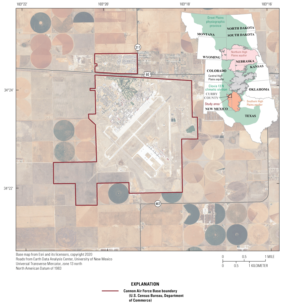
Aerial imagery of the general study area, Cannon Air Force Base, and surrounding lands within Curry County, New Mexico.
In 2020, the U.S. Geological Survey (USGS), in cooperation with the U.S. Air Force Civil Engineer Center, developed a potentiometric surface contour map of winter 2020 groundwater levels documenting the altitude of the water table and groundwater-flow patterns of the Southern High Plains aquifer on and around Cannon AFB. The objectives of the current study are to assist Cannon AFB in understanding and interpreting current and local hydrologic conditions and to evaluate groundwater-level change from 2015 to 2020 using new and historical data. The potentiometric surface can be used to better understand the hydrologic conditions of the Southern High Plains aquifer within the study area. Analysis of groundwater-flow directions and hydraulic gradients can provide an understanding of depletion by heavy groundwater pumping and recharge through playa lakes, as well as the relationship between the groundwater levels and underlying geology.
Purpose and Scope
The purpose of this report is to present the results of a groundwater-level survey completed in winter 2020 by means of potentiometric surface contour maps of winter 2020 groundwater levels and present an analysis of the potentiometric surface. Recent (2015–20) groundwater-level change was also evaluated by constructing a map showing the change in groundwater level between the winter 2015 and winter 2020 measuring events. Four hydrographs presented herein, created from periodic measurements of groundwater levels in wells on and around Cannon AFB, were developed to provide information about historical groundwater-level changes and provide localized data to assist in understanding regional trends.
Hydrogeology
The groundwater hydrology of the Southern High Plains aquifer in the Cannon AFB area is primarily controlled by recharge characteristics, groundwater withdrawals, and the contact between the saturated Ogallala Formation and the underlying Dockum Group (Chinle Formation). The Dockum Group and Chinle Formation have been used interchangeably in the past to refer to the uppermost rocks underlying the Ogallala Formation; the Chinle Formation is the uppermost unit of the Dockum Group. Although most recent literature has transitioned to using the more general term “Dockum Group,” some references cited in this report include the use of the term “Chinle Formation” (Collison, 2016; McGowen and others, 1977). For continuity and to reduce confusion, this report uses the term “Dockum Group” throughout. Groundwater levels have substantially declined throughout the Southern High Plains aquifer since the mid-1940s, when groundwater was first used for irrigated agriculture (McGuire and others, 2003; Tillery, 2008). Groundwater used for drinking water and irrigation in this region occurs in the Ogallala Formation that is part of the Southern High Plains aquifer. The contact between the Ogallala Formation and the Dockum Group contact provides the main control for regional aquifer conditions in the aquifer, and pumping likely has a strong effect on local conditions. The Ogallala Formation was deposited on top of an eastward-dipping erosional surface containing paleochannels that cut into the Dockum Group (Dutton and others, 2001). These paleochannels contain coarser, more hydraulically conductive sediment than the sediment found in the underlying Dockum Group and can act as preferential pathways for groundwater movement. The paleochannels generally coincide with troughs in the water-table surface.
The Dockum Group consists mostly of clay with some intermixed sand and silt and ranges in thickness from 0 to 400 feet (ft) in eastern New Mexico (McGowen and others, 1977). The Ogallala Formation consists of aeolian sand and silt and fluvial and lacustrine sand, silt, clay, and gravel (McLemore, 2001) and ranges in thickness from 30 to 600 ft in eastern New Mexico and west Texas (Gustavson, 1996). The Blackwater Draw Formation overlies the Ogallala Formation at Cannon AFB, is composed mostly of eolian sand deposits, and ranges in thickness from 0 to 80 ft in eastern New Mexico (McLemore, 2001). A laterally discontinuous caliche layer is typically present in the unsaturated zone of the Blackwater Draw or Ogallala Formations (Hart and McAda, 1985). Drilling at Cannon AFB has indicated the caliche layer is discontinuous but typically found within 30 ft of the surface and of variable thickness when present (Langman and others, 2006).
Recharge to the Southern High Plains aquifer has previously been estimated to range from 0.01 inch per year (in/yr) (Stone and McGurk, 1985) to 1.71 in/yr (Mantei and others, 1966–67); but most estimates are less than 1 in/yr (Musharrafieh and Logan, 1999). It has long been debated how the aquifer is recharged, but the current conceptual model indicates that most recharge occurs through playa areas and that interplaya areas contribute very little to aquifer recharge (Scanlon and others, 2003). Potential evapotranspiration in excess of precipitation likely limits diffused areal recharge (Langman and others, 2006). Groundwater pumping in the area has occurred since the early 1900s, but large-scale agriculture did not develop near the study area until the 1950s (Musharrafieh and Logan, 1999). Groundwater in the Southern High Plains aquifer generally flows eastward or southeastward, which is consistent with the overall direction of regional flow in the unconfined aquifer surrounding Cannon AFB. Groundwater pumping has created numerous cones of depression that have locally reversed groundwater-flow gradients around heavily irrigated areas.
Methods
Hydrographs
Four hydrographs were created from periodic measurements of groundwater levels in wells on and around Cannon AFB (USGS, 2020) and were developed to provide information about historical groundwater-level changes. The hydrographs of well IDs 4, 76, 81, and 108 were created using R programming language, version 4.0.2 (R Core Team, 2020). The hydrographs were created for four wells with the most complete and longest running groundwater-level records and were selected to represent areas on and around Cannon AFB. The wells used to create the hydrographs are similar to those in Collison (2016), except for well 26, which was inaccessible in winter 2020. Groundwater levels at these four wells are measured up to twice a year by the USGS in cooperation with the New Mexico Office of State Engineer. Data from AFSOC (2013) were used to fill in a gap from 2005 to 2013 at Cannon AFB well 81.
Potentiometric Surface Contour Map
The potentiometric surface contour map of the study area was constructed using the groundwater-level altitudes presented in table 1. Groundwater-level measurements were attempted at 155 sites during a nonirrigation season (winter of 2020; January 13–31, 2020). Irrigation, domestic, and monitoring wells within approximately 6 miles of the Cannon AFB boundary were selected for measurement. Although we tried to measure groundwater levels in all wells that were measured in the 2015 survey, some wells were not accessible in 2020. The wells measured in this study were assumed to be screened in the Ogallala Formation, with the total depth of the wells generally coinciding with the top of the Dockum Group. This assumption is based on drilling logs, a previous USGS report (Collison, 2016), and discussions with local farmers and drillers. Well identifiers (IDs) 2 through 129 are numbered in accordance with wells that were accessible and in Collison (2016), whereas well IDs 200 through 232 are new locations that were added to fill in data gaps and improve the accuracy of the potentiometric surface. Some measurements may have been affected by recent pumping before they were made, although groundwater levels were not measured in wells that were pumping. The presence of nearby pumping was noted on field forms, and those wells were not used in the development of the potentiometric surface. Additionally, for wells encountered that were pumping, notes were taken on field forms and the wells were revisited on a separate date when the well wasn’t pumping. In total, 112 wells measured during the 2020 survey were used to construct the potentiometric surface: 75 irrigation wells, 15 domestic wells, and 22 monitoring wells; of these, 3 irrigation wells and 1 monitoring well have associated hydrographs presented later herein.
An additional groundwater-level survey was conducted in March 2021 and used as a testing mechanism to validate previously collected data and to provide additional support for determining flow directions through Cannon AFB. Groundwater levels were measured during a nonirrigation season at 31 wells, 10 of which produced a valid measurement; the rest were either pumping, obstructed, or dry. These wells were not used in the creation of the potentiometric surface but as a secondary validation in areas of high concern.
Groundwater-level measurement and quality-control procedures set forth by Cunningham and Schalk (2011) were followed; specifically, a minimum of two groundwater-level measurements that were within 0.02 ft of each other were required at each well measured. Data collected for this study are available from the USGS National Water Information System (NWIS) database (https://nwis.waterdata.usgs.gov/usa/nwis/gwlevels) (USGS, 2020).
Land surface datums were updated for the 2020 groundwater-level measurements in conjunction with a separate geophysical logging project by the USGS at Cannon AFB (Payne and others, 2022). This will allow future work in the area to assume a uniform digital elevation model for collaborative work and create the framework for future products and ArcGIS surfaces within Cannon AFB. Land surface datum measurement corrections were retroactively applied to well locations measured during the 2015 event that overlapped with locations of wells used in this report. The new 1-meter (m) resolution digital elevation model altitudes were obtained from The National Map and are referenced to the North American Vertical Datum of 1988 (USGS, 2019).
Table 1.
Inventory of sites and associated groundwater data used to construct winter 2015 and winter 2020 potentiometric surface contour maps and water-level change maps for the Cannon Air Force Base (AFB) area, Curry County, New Mexico.[Map identification number corresponds to those shown on figures in this report. Well type: D, domestic, I, irrigation, MW, monitoring well (followed, if applicable, by name of well on Cannon AFB); Map identification numbers shown in bold indicate an associated hydrograph is provided for these wells. USGS, U.S. Geological Survey; NAD 83, North American Datum of 1983; NAVD 88, North American Vertical Datum of 1988. Land surface datum for 2020 and 2015 have been updated and this table reflects new groundwater-level altitudes]
The potentiometric surface contour map was constructed by interpolating between measurement locations using universal kriging (Fisher, 2013). This approach estimates the values at unmeasured locations as a weighted average of measured values. The weights are derived from the spatial correlation of measurements, as indicated by an empirical semivariogram (Fisher, 2013). Kriging assumes stationarity, where the mean value of the data being contoured and the empirical semivariogram are roughly constant throughout the area of interest. A first-order polynomial trend function representative of the regional groundwater-level altitude trend was subtracted from the measured values during semivariogram modeling and kriging to favor stationarity. The removed trend was formulated as
wherez(s)
is groundwater-level altitude at point s, in feet above the North American Vertical Datum of 1988;
β0
is deterministic unknown trend coefficient, in feet above the North American Vertical Datum of 1988;
βi
is deterministic unknown trend coefficient, in dimensionless units (i = 1 through 5);
x(s)
is easterly coordinate at point s, in feet; and
y(s)
is northerly coordinate at point s, in feet.
The trend was added back to the kriged surface to arrive at the potentiometric surface. The kriging analysis was performed by using the R programming language, version 4.0.2 (R Core Team, 2020). Points of equal hydraulic head in the potentiometric surface were connected to form contour lines used for visualization of the surface. The Pearson correlation coefficient of the trend predictions to measurements is 0.91, indicating large-scale regional trends were reasonably represented. Normally distributed residuals (measured minus predicted) had a mean of 0 ft and median of 0.12 ft, thereby suggesting an acceptable level of spatial stationarity to validate the application of kriging. The final contoured area was restricted to the perimeter of groundwater-level measurements to avoid universal kriging estimation errors introduced by low data density on the margins of the study area.
The empirical semivariogram is a graphical representation of how variances in measured values (in terms of semivariance) change as a function of distance between the measurement locations (separation distance). A continuous semivariogram model was fit to the curvature of the empirical semivariogram to provide a data-driven method for kriging to estimate spatial correlation at all separation distances. The semivariogram model has four primary attributes: model type, sill, range, and nugget. The model type defines the overall shape of the semivariogram model and will change depending on how rapidly measured values change as a function of separation distance. Semivariance in semivariograms typically levels off at a certain separation distance, beyond which there is minimal spatial correlation between measured and unmeasured locations. This distance is called the range, and the semivariance value that the semivariogram levels off at is called the sill. The nugget is the semivariance at a separation distance of zero, or y-intercept of the semivariogram model, and is therefore typically related to measurement error.
The empirical semivariogram in this study was calculated by using the variogram function within the gstat R package, version 2.0-0 (Pebesma and Graeler, 2019). The maximum distance considered in the empirical semivariogram was 10,000 m, or approximately half the maximum distance between observation locations (24,140.2 m; Fisher, 2013), which is greater than both the mean (7,203.3 m) and median (6,790.3 m) distance between all observation pairs. A bin width of 500 m was used in the empirical semivariogram calculation, since it yielded the most readily identifiable semivariogram curvature (20 bins of maximum separation distance). The fit.variogram function of the gstat R package was then used to fit a continuous semivariogram model to the empirical semivariogram. The resulting semivariogram model was of spherical type, with a range of 7,444.8 m, a sill of 640.2 square feet, and a nugget of 0 square feet (fig. 2). The modeled semivariogram well-represents the general curvature of the empirical semivariogram, as evidenced by their Pearson correlation coefficient of 0.84.
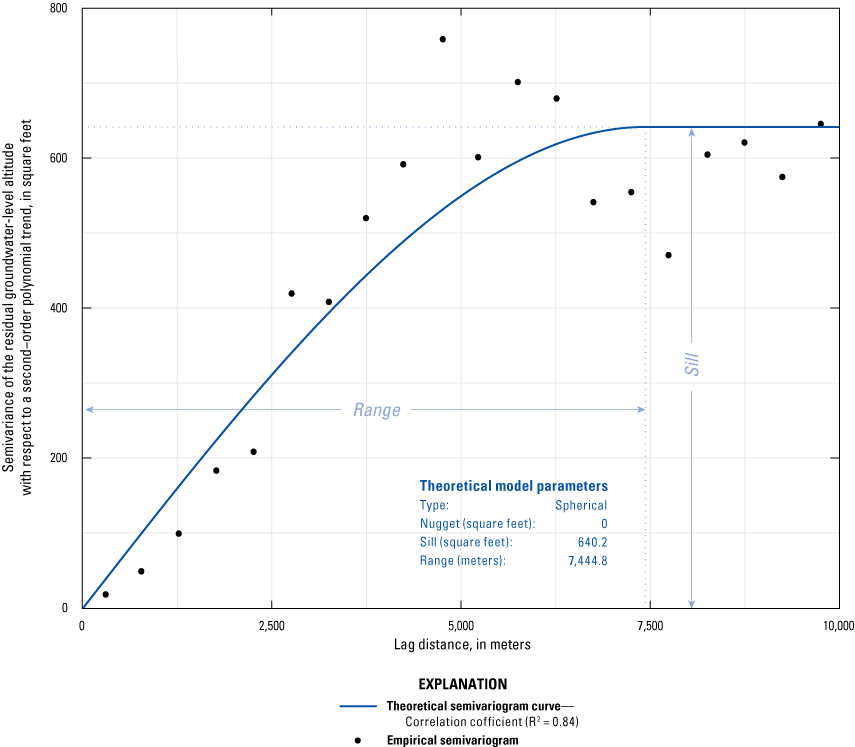
Empirical semivariogram fit with continuous spherical variogram model.
Kriging was then performed by using the krige function within the gstat R package to estimate the potentiometric surface on a uniform raster grid. Interpolated root-mean-square error (RMSE) at measured locations decreased as a function of raster grid cell size. A uniform grid cell size of 15 ft was selected as a tradeoff between raster file size and RMSE. Measured values were very well represented by kriged raster predictions, with an RMSE of 0.029 ft, a Pearson correlation coefficient of 1.00, a mean residual of 0.001 ft, and a median residual of 0.0019 ft. The resulting potentiometric surface contour map will be discussed and presented in the results section of this report.
Leave-one-out cross validation (LOOCV) was performed to further evaluate the predictive capabilities of the kriging approach. LOOCV provides insight into predictive capability by removing one data point, kriging the remaining data, and computing kriged prediction error at the removed location. This process is repeated for all measurement locations. LOOCV was performed by using the RunCrossValidation function within the ObsNetwork R package, version 1.0.1.9000 (Fisher, 2013). Mean LOOCV error (measurements minus LOOCV predictions) would ideally be zero and was −0.145 ft in the analysis, indicating the kriging approach had a high-level of predictive ability with a small bias toward overpredicting groundwater-level altitudes. The high level of predictive ability of the kriging approach is further emphasized by the low negative correlation of −0.0903 between LOOCV predictions and prediction error, as well as the high correlation of 0.986 between measured groundwater-level altitudes and LOOCV predictions (fig. 3). Sites with more than 25 ft of LOOCV error included site 21 (−59.63 ft), site 200 (−41.99 ft), site 97 (27.60 ft), and site 55 (37.24 ft). Most of these sites are located within a short distance of the paleochannels where groundwater-level altitudes spatially vary more across a given distance than elsewhere in the area. This indicates a greater sensitivity to data density and elevated prediction uncertainty in this area. Overall, the kriged solution performed well and is thought to reasonably estimate the potentiometric surface throughout the area of interest; however, by using a new geophysical surface created by the USGS that represents the top of the Dockum Group and bottom of the Ogallala Formation, we were able to modify the 3,980-, 3,990-, 4,000-, and 4,010-ft potentiometric contour lines just north of Cannon AFB in areas where groundwater-level data were sparse. This surface along with the March 2021 groundwater-level survey allowed us to predict groundwater flow with greater accuracy than possible by using kriging alone.
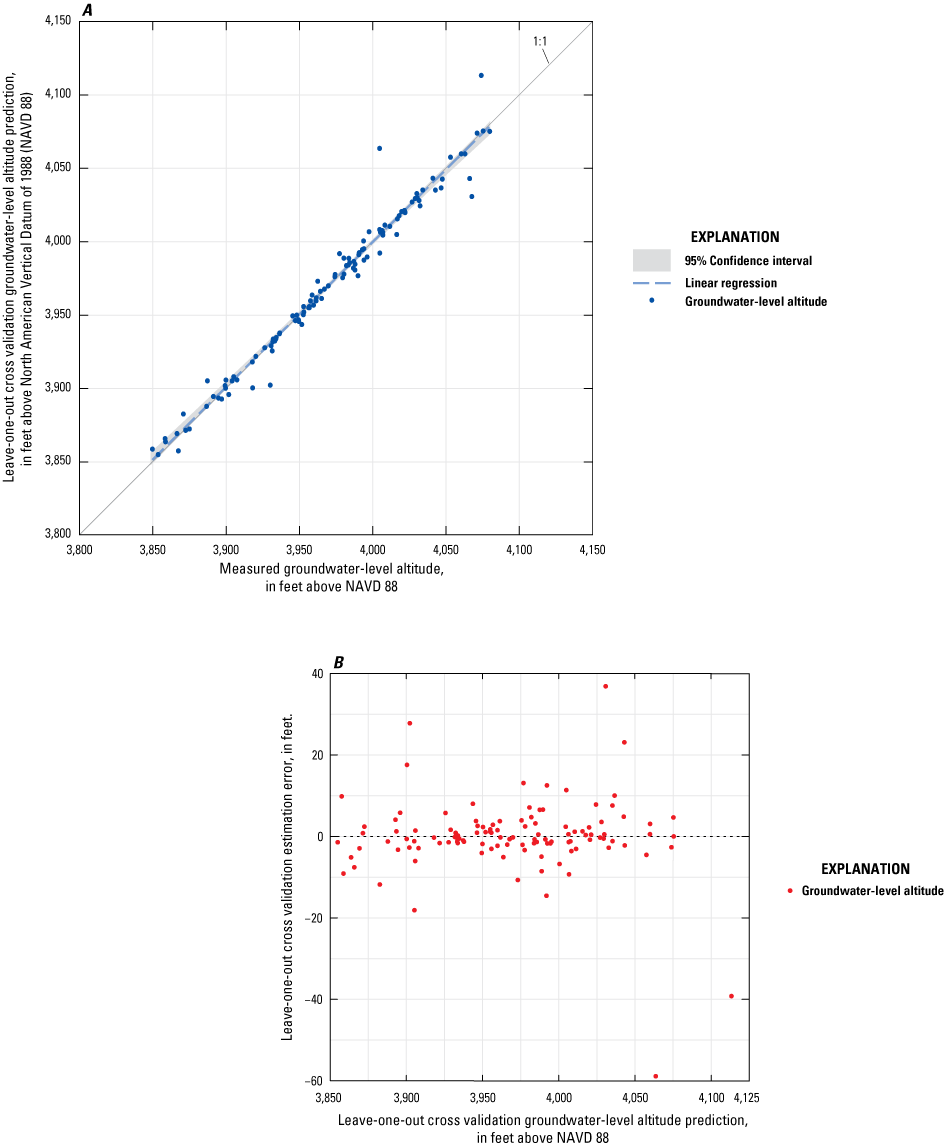
A, Leave-one-out cross validation (LOOCV) predictions verses measurements and, B, LOOCV estimation errors verses LOOCV predictions (bottom).
Groundwater-Level Change Map
Of the 112 wells measured in this report, 67 were also measured in 2015. Groundwater-level change values (winter 2020 minus winter 2015 groundwater-level altitude) were computed at 67 well sites having groundwater-level measurements in 2015 and 2020. ArcGIS 10.7.1 was used to interpolate a groundwater-level change surface from the well points using the natural-neighbor method with an output cell size of 5.7078 × 10⁻⁴ (Childs, 2004). The groundwater-level change surface was divided into six groups (1) greater than or equal to a 1.1-ft increase to indicate a rise in groundwater level, (2) between 1.0 to −1.0 ft to indicate a neutral change in groundwater level, and (3–6) between −1.1 to −5.0 ft, −5.1 to −10.0 ft, −10.1 to 15.0 ft, and −15.1 to −17.6 ft to indicate a decline in groundwater level. The six groups were visually inspected for reasonability and corrected as necessary.
Results and Discussion
Hydrographs
The period of record for the four hydrographs ranges from 27 years (well 81) to 66 years (wells 4 and 76; fig. 4). The long-term trend present in all four hydrographs is a steady decline in groundwater levels, with water levels in some wells declining faster than others. The decadal differences in rates of decline mentioned in Collison (2016) are still apparent at wells 4, 76, and 108, which indicates less groundwater decline or static groundwater-level conditions during the mid- to late 1980s, possibly related to an above average period of precipitation from 1984 to 1988 (fig. 5). The hydrographs also appear to show less groundwater decline or static groundwater-level conditions from 2013 through 2020 at wells 4, 76, 81, and 108 (fig. 4).
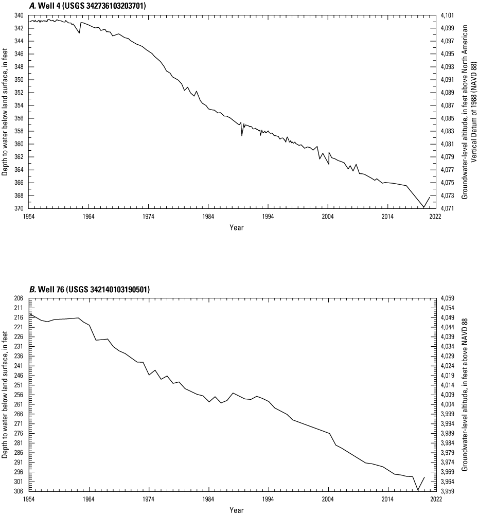
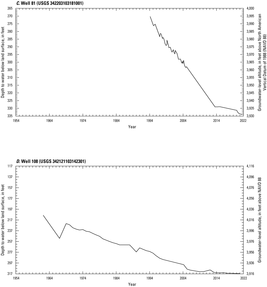
Groundwater-level altitude hydrographs from selected wells on and around Cannon Air Force Base, Curry County, New Mexico, 1954–2020.
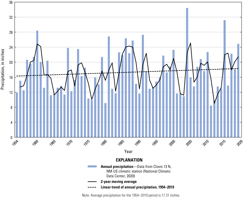
Annual average precipitation in Clovis, New Mexico, 1954–2020. Data from National Climatic Data Center (2020), Clovis 13N climatic station.
Well 4 data indicate water levels have declined since the mid-1960s, including a sharp 3.7-ft decline between 2017 and 2020 (fig. 4); however, remarks made in NWIS indicate that the technicians may have obtained a poor water-level measurement that may account for the steep drop. Well 76 data show an overall decline since 1954 with a brief rebound in 2018 (fig. 4), but remarks on the 2019 water-level measurement show difficulties associated with collecting the measurement. Future water-level recordings may confirm that the above average precipitation in Clovis from 2015 to 2019, excluding 2016, and conscious water conservation practices, may be responsible for a less pronounced groundwater decline, compared to prior years, or near-static groundwater-level conditions.
Well 81, in the southeastern corner of Cannon AFB, had the largest average annual groundwater-level decline of approximately 2.36 feet per year (ft/yr) (fig. 4). Well 108, east-southeast of Cannon AFB, had the second largest decline in average annual groundwater levels of 1.87 ft/yr. Well 76, directly south of Cannon AFB, had the third largest average annual groundwater-level decline of 1.28 ft/yr (fig. 4). Lastly, well 4, north-northwest of Cannon AFB, had the smallest average annual groundwater-level decline of approximately 0.44 ft/yr (fig. 4). Overall, the southern part of the study area exhibited the greatest average annual groundwater-level decline, with decline also occurring in the northwest portion of the study area. Collison (2016) showed the northwestern part of the study area having the smallest average annual decline, with the northeastern part having similar declining values.
Potentiometric Surface Contour Map
The January 13–31, 2020, potentiometric surface representing winter groundwater conditions, as well as interpreted groundwater-flow directions, are both illustrated in figures 6 and 7 (on sheet). The groundwater-flow directions were derived by using the hydrologic principle that groundwater flows in the direction of the steepest hydraulic gradient (from high to low hydraulic head), perpendicular to contour lines of equal hydraulic head (Ingebritsen and others, 2006). The potentiometric surface indicates that groundwater flows from the northwest toward the southeast, following a mesoscopic regional trend pattern indicated by Langman and others (2006). The potentiometric surface also shows groundwater flow from the north and west converging on a trough in the potentiometric surface. This groundwater trough is thought to be the hydraulic expression of a Tertiary paleochannel, commonly found in the Southern High Plains aquifer (Gustavson, 1996), which contains coarser, more hydraulically conductive material than the underlying formation (Fahlquist, 2003).
Although regional groundwater-flow directions are similar for winter 2020 and winter 2015 (Collison, 2016), there are local differences between the maps. The potentiometric contours along the west and north borders of Cannon AFB shifted with the addition of the top of the Dockum Group surface as a reference. The addition of a groundwater measurement in the northwest corner (well 200) provides a more complete picture of the water table, which now shows a cone of depression around well 21 and an increase in the distances between potentiometric surface contours in the northwest part of the study area (fig. 6, on sheet). Slight differences between the winter 2020 and winter 2015 potentiometric contours may be, in part, due to different interpolation methods that were used for the two studies as well as small deviations in the surface contours, because it was not possible to measure the exact same wells in 2020 as in 2015, owing to access and pumping issues. The kriging interpolation used in this study, supported by the statistical analysis, provides a more representative potentiometric surface than the standard natural neighbor interpolation method used in the previous study (Collison, 2016).
Groundwater-Level Change Map
The groundwater-level change map (fig. 8, on sheet) shows a visual representation of the change in groundwater level from winter of 2015 to winter of 2020 measuring events and includes 67 wells whose data were used to construct the map. The periods between both groundwater-level measurement events contained several cycles of increased irrigation pumping and winter dormancy. The largest groundwater-level rise occurred in the southeastern section of the study area (6.74 ft) and the second largest rise occurred just north of the base (5.51 ft). The mean groundwater-level change for the 67 wells measured is approximately −1.12 ft. Much of the area measured, covering 34 out of 67 wells, shows declining water levels ranging from −1.1 to −17.6 ft. The 20 groundwater-level changes that range from −1.0 to 1.0 ft are considered neutral, with levels neither declining nor rising, and only 13 out of 67 wells measured show rising water levels ranging from 1.28 to 6.74 ft. Of the wells that were included in both the 2015 and 2020 winter surveys, 50.7 percent show a decline, 29.9 percent are neutral, and 19.4 percent show a rise. Most of the wells showing a groundwater-level rise were in the region to the north of U.S. Highway 60, whereas most of the wells showing groundwater-level declines were in the regions south of the highway and just west of Clovis.
Summary
This study was conducted by the U.S. Geological Survey, in cooperation with the U.S. Air Force Civil Engineer Center, to assist Cannon Air Force Base in understanding and interpreting current and local hydrologic conditions and to evaluate groundwater-level change from 2015 to 2020 using new and historical data. Groundwater-level data collected in 2015 and 2020 indicate that water levels have declined over much of the study area during this 5-year period. The long-term trend in all four hydrographs was a steady decline in groundwater levels, with some areas declining faster than others. Overall, the southern part of the study area exhibited the greatest average annual groundwater-level decline, with declining levels also present in the northwestern and northeastern portions of the study area. However, decadal differences in rates of decline that show less groundwater decline or static groundwater-level conditions during the mid- to late 1980s at wells 4, 76, and 108 were also present from 2013 through 2019 at wells 4, 76, 81, and 108. Future water-level data may confirm that the above average precipitation in Clovis, New Mexico, from 2015 to 2019, excluding 2016, and conscious water conservation practices, may be responsible for less dramatic groundwater decline or near static groundwater-level conditions, when compared to prior years.
The potentiometric surface map indicates that groundwater flows from the northwest toward the southeast, following a megascopic regional pattern as indicated by an earlier study. The map also shows groundwater flow from the north and west converging on a trough in the potentiometric surface. The slight differences between the winter 2020 and winter 2015 potentiometric contours may be, in part, due to a different interpolation method used in the current study relative to the preceding study. The kriging interpolation used in this study, however, supported by the statistical analysis, provided a more representative potentiometric surface than other interpolation methods.
The 67 corresponding wells measured in 2015 and 2020 were used to create the groundwater-level change map. Of these wells, 50.7 percent showed a water-level decline, 29.8 percent indicated neutral water levels, and 19.4 percent indicated a rise in water levels. The region north of U.S. Highway 60 contained most of the groundwater-level rise, whereas the regions located south of the highway and just west of Clovis, N. Mex., contained most of the groundwater-level decline.
Long-term water-level monitoring during periods of substantial land-use change is helpful to assess changes in aquifers. Monitoring the effects of climate variability, regional effects of groundwater development, changes in flow direction, groundwater and surface-water interactions, as well as future groundwater-level surveys and potentiometric surface maps, would provide resource managers with important information to aid in the decision process.
References Cited
Air Force Special Operations Command [AFSOC], 2013, 2012 Biennial groundwater monitoring and annual landfill inspection report—Landfills LF-03, LF-04, LF-05, LF-25, and former sewage lagoons Cannon Air Force Base, New Mexico: New Mexico Environment Department, prepared by Bhate Environmental Associates, Inc., and Trinity Analysis & Development Corp., accessed February 6, 2023, at https://hwbdocuments.env.nm.gov/Cannon AFB.
Childs, C., 2004, Interpolating surfaces in ArcGIS spatial analyst: Arc User, July–September 2004, p. 32–35, accessed June 2020 at http://www.esri.com/news/arcuser/0704/files/interpolating.pdf.
Collison, J., 2016, Potentiometric surfaces, summer 2013 and winter 2015, and select hydrographs for the Southern High Plains aquifer, Cannon Air Force Base, Curry County, New Mexico: U.S. Geological Survey Scientific Investigations Map 3352, 2 sheets, accessed March 17, 2023, at https://doi.org/10.3133/sim3352.
Cunningham, W.L., and Schalk, C.W., comps., 2011, Groundwater technical procedures of the U.S. Geological Survey: U.S. Geological Survey Techniques and Methods, book 1, chap. A1, 151 p., accessed March 17, 2023, at https://pubs.usgs.gov/tm/1a1/.
Dutton, A.R., Mace, R.E., and Reedy, R.C., 2001, Quantification of spatially varying hydrogeologic properties for a predictive model of groundwater flow in the Ogallala aquifer, northern Texas panhandle, in Lucas, S.G., and Ulmer Scholle, D.S., eds., Geology of Llano Estacado: Socorro, N. Mex., New Mexico Geological Society, p. 297–307.
Fahlquist, L.S., 2003, Ground-water quality of the Southern High Plains aquifer, Texas and New Mexico, 2001: U.S. Geological Survey Open-File Report 2003–345, 59 p., accessed May 2015 at http://pubs.er.usgs.gov/publication/ofr03345.
Gustavson, T.C., 1996, Fluvial and eolian depositional systems, paleosols, and paleoclimate of the upper Cenozoic Ogallala and Blackwater Draw Formations, Southern High Plains, Texas and New Mexico: Austin, Tex., Bureau of Economic Geology, University of Texas, Report of Investigations No. 239, 62 p., accessed March 17, 2023 at https://doi.org/10.23867/RI0239D.
Hart, D.L., and McAda, D.P., 1985, Geohydrology of the High Plains aquifer in southeastern New Mexico: U.S. Geological Survey Hydrologic Investigations Atlas 679, 1 sheet, accessed March 17, 2023, at https://doi.org/10.3133/ha679.
Langman, J.B., Falk, S.E., Gebhardt, F.E., and Blanchard, P.J., 2006, Groundwater hydrology and water quality of the Southern High Plains aquifer: U.S. Geological Survey Scientific Investigations Report 2006–5280, 61 p., accessed March 17, 2023, at https://doi.org/10.3133/sir20065280.
McGowen, J.H., Granata, G.E., and Seni, S.J., 1977, Depositional systems, uranium occurrence, and postulated ground-water history of the Triassic Dockum Group, Texas Panhandle—Eastern New Mexico: Austin, Tex., University of Texas, Bureau of Economic Geology, 104 p., accessed March 17, 2023, at https://www.beg.utexas.edu/files/publications/cr/CR1977-McGowen-1-QAe5601.pdf.
McGuire, V.L., Johnson, M.R., Schieffer, R.L., Stanton, J.S., Sebree, S.K., and Verstraeten, I.M., 2003, Water in storage and approaches to groundwater management, High Plains aquifer, 2000: U.S. Geological Survey Circular 1243, 51 p., accessed March 17, 2023, at https://doi.org/10.3133/cir1243.
Miller, J.A., ed., 2000, Groundwater atlas of the United States: U.S. Geological Survey Hydrologic Atlas 730, 13 chap., accessed November 23, 2020, at https://pubs.usgs.gov/ha/730c/report.pdf.
Musharrafieh, G.R., and Logan, L.M., 1999, Numerical simulation of groundwater flow for water rights administration in the Curry and Portales Valley underground water basins, New Mexico: Santa Fe, N. Mex., New Mexico Office of the State Engineer, Technical Division Hydrology Bureau Report 99–2, 169 p., accessed March 17, 2023, at https://hwbdocuments.env.nm.gov/Cannon%20AFB/1999-03-01%20Numerical%20Simulation%20of%20GW%20Flow%20for%20Water%20Rights.pdf.
National Climatic Data Center, 2020, Climate data online, monthly summaries, Clovis, NM: National Oceanic and Atmospheric Administration, National Centers for Environmental Information web page, accessed September 1, 2020, at https://www.ncdc.noaa.gov/cdo-web/datasets/GSOM/stations/GHCND:USC00291963/detail.
Payne, J.D., Teeple, A.P., McDowell, J., Wallace, D., and Hancock, W.A., 2022, Mapping the altitude of the top of the Dockum Group and paleochannel analysis using surface geophysical methods on and near Cannon Air Force Base in Curry County, New Mexico, 2020: U.S. Geological Survey Scientific Investigations Report 2022–5050, 21 p., accessed March 17, 2023, at https://doi.org/10.3133/sir20225050.
Pebesma, E., and Graeler, B., 2019, Package ‘gstat’—Spatial and spatio-temporal geostatistical modelling, prediction and simulation (ver. 2.0–8): Comprehensive R Archive Network (CRAN) software release, accessed May 30, 2020, at https://cran.r-project.org/web/packages/gstat/gstat.pdf.
R Core Team, 2020, R—A language and environment for statistical computing: Vienna, Austria, R Foundation for Statistical Computing, accessed May 12, 2020, at https://www.R-project.org/.
Scanlon, B.R., Angle, E.S., Christian, B., Pi, J., Martinez, K., Reedy, R., Boghici, R., and Petrossian, R., 2003, Evaluation of enhanced recharge potential to the Ogallala aquifer in the Brazos River Basin, Hale County, Texas: Texas Water Development Board Report 355, 66 p., accessed March 17, 2023, at https://www.twdb.texas.gov/publications/reports/numbered_reports/doc/R355/Report355.pdf.
Stone, W.J., and McGurk, B.E., 1985, Ground-water recharge on the Southern High Plains, east-central New Mexico, in Lucas, S.G., and Zidek, J., eds., Guidebook of Santa Rosa Tucumcari region, 36th Field Conference: Socorro, N. Mex., New Mexico Geological Society, p. 331–335., accessed March 17, 2023, at https://nmgs.nmt.edu/publications/guidebooks/downloads/36/36_p0331_p0335.pdf.
U.S. Geological Survey [USGS], 2019, 3D elevation program 1-meter resolution digital elevation model (June 6, 2020): U.S. Geological Survey web page, accessed March 17, 2023, at https://data.usgs.gov/datacatalog/data/USGS:77ae0551-c61e-4979-aedd-d797abdcde0e.
U.S. Geological Survey [USGS], 2020, USGS water data for the Nation: U.S. Geological Survey National Water Information System database, accessed August 3, 2020, at https://doi.org/10.5066/F7P55KJN.
Datum
Vertical coordinate information is referenced to the North American Vertical Datum of 1988 (NAVD 88).
Horizontal coordinate information is referenced to the North American Datum of 1983 (NAD 83).
Altitude, as used in this report, refers to distance above the vertical datum.
For more information about this publication, contact
Director, New Mexico Water Science Center
U.S. Geological Survey
6700 Edith Blvd. NE
Albuquerque, NM 87113
For additional information, visit
https://www.usgs.gov/centers/nm-water
Publishing support provided by
Lafayette Publishing Service Center
Disclaimers
Any use of trade, firm, or product names is for descriptive purposes only and does not imply endorsement by the U.S. Government.
Although this information product, for the most part, is in the public domain, it also may contain copyrighted materials as noted in the text. Permission to reproduce copyrighted items must be secured from the copyright owner.
Suggested Citation
Goodwin, A.B., and Bell, M.T., 2023, Potentiometric surface map of the Southern High Plains aquifer in the Cannon Air Force Base area, Curry County, New Mexico, 2020: U.S. Geological Survey Scientific Investigations Map 3504, 1 sheet, 18-p. pamphlet, https://doi.org/10.3133/sim3504.
ISSN: 2329-132X (online)
Study Area
| Publication type | Report |
|---|---|
| Publication Subtype | USGS Numbered Series |
| Title | Potentiometric surface map of the Southern High Plains aquifer in the Cannon Air Force Base area, Curry County, New Mexico, 2020 |
| Series title | Scientific Investigations Map |
| Series number | 3504 |
| DOI | 10.3133/sim3504 |
| Publication Date | June 15, 2023 |
| Year Published | 2023 |
| Language | English |
| Publisher | U.S. Geological Survey |
| Publisher location | Reston, VA |
| Contributing office(s) | New Mexico Water Science Center |
| Description | Report: vi, 18 p., Dataset; 1 Sheet: 21.00 × 28.00 inches |
| Country | United States |
| State | New Mexico |
| County | Curry County |
| Other Geospatial | Cannon Air Force Base area |
| Online Only (Y/N) | Y |