

Characterization of Ambient Groundwater Quality Within a Statewide, Fixed-Station Monitoring Network in Pennsylvania, 2015–19
Links
- Document: Report (13.7 MB pdf) , HTML , XML
- Data Release: USGS data release - Data for characterization of ambient groundwater quality within a state-wide, fixed station monitoring network in Pennsylvania, 2015–2019
- NGMDB Index Page: National Geologic Map Database Index Page (html)
- Download citation as: RIS | Dublin Core
Acknowledgments
This study was funded by an ongoing cooperative effort between the U.S. Geological Survey (USGS) Pennsylvania Water Science Center and the Pennsylvania Department of Environmental Protection (PaDEP). The authors would like to thank Susan Weaver and Amy Williams of PaDEP for their assistance and guidance in operation of the network. Appreciation is extended to the local land managers, including the staff of the Pennsylvania Department of Conservation and Natural Resources and the Pennsylvania Game Commission for their cooperation in maintaining access to sampling locations. Thanks are extended to USGS colleagues Mitchell Weaver, Kyle Ohnstad, Dennis Low, and Dana Heston for groundwater sampling, and Brandon Fleming, Chuck Cravotta, and James Degnan for report reviews.
Abstract
Pennsylvania leads the Nation in the number of individuals that use groundwater for private domestic water supply; more than 3 million rural and suburban Pennsylvania residents rely on private domestic supplies for drinking water. These supplies are not regulated nor routinely monitored; thus relevant groundwater-quality information is not widely available. The U.S. Geological Survey (USGS), in cooperation with the Pennsylvania Department of Environmental Protection (PaDEP) Safe Drinking Water Bureau, established a statewide, fixed-station ambient groundwater quality network in 2015. The goals for the Pennsylvania Groundwater Monitoring Network (GWMN) include characterizing ambient groundwater quality conditions in rural areas of the State and documenting potential changes in conditions over time. Seventeen wells were selected for monitoring at 6-month intervals beginning in 2015. Since then, several wells have been added to the GWMN, bringing the total number of wells sampled in the fall of 2019 to 28. Routinely monitored constituents included physical characteristics and chemical concentrations in filtered and unfiltered samples (major and trace elements, nutrients, and organic compounds). Samples for volatile organic compounds (VOCs), radionuclides, and dissolved hydrocarbon gases were collected during the first sampling event at each well.
To offer insights on the quality of groundwater used for domestic supply in Pennsylvania, summary statistics for the 221 GWMN samples collected during 2015–19 are compared to U.S. Environmental Protection Agency (EPA) drinking-water standards, which are applicable to public water supplies. Results show that samples across the GWMN generally meet drinking-water standards for inorganic and organic constituents; however, a percentage of samples had concentrations that exceeded maximum contaminant level (MCL) thresholds for nitrate (3 percent) and secondary maximum contaminant level (SMCL) thresholds for iron (32 percent), manganese (36 percent), and aluminum (5 percent). Radon-222 activities, which were sampled only during the initial visit to a well, exceeded the lower proposed drinking water standard of 300 picocuries per liter (pCi/L) in 64 percent of wells in the GWMN; additionally, 7 percent of wells exceeded the higher proposed standard of 4,000 pCi/L. There were no exceedances for VOCs, but one well had a tribromomethane detection. Three wells had detectable concentrations of methane, with one sample exceeding the Pennsylvania action level of 7 milligrams per liter (mg/L).
The pH and dissolved oxygen concentrations varied widely across the GWMN and were correlated with dissolved metal concentrations and other chemical characteristics of groundwater samples. Considering all samples collected for the study, the pH ranged from 4.2 to 8.3; 42 percent of pH values were either above or below the SMCL range of 6.5–8.5. The highest pH values resulted from contamination of loose grout used in the construction of one well and decreased to levels consistent with other wells in the vicinity after repeated sampling rounds. Dissolved oxygen (DO), which ranged from 0 to 13.9 mg/L, influences the mobility and prevalence of constituents with variable oxidation state, including iron, manganese, and nitrogen species. Samples with acidic pH (less than 6.5) and (or) low DO had the highest concentrations of manganese and iron, whereas those with neutral to alkaline pH values had the highest concentrations of calcium, magnesium, sodium, and other major ions. Analysis of major ions indicates that calcium/bicarbonate water types are the most common, with a few characterized as calcium/chloride or sodium/chloride, and most others as mixed water types including calcium-magnesium/bicarbonate, sodium-magnesium/bicarbonate, and sodium/bicarbonate-chloride.
Nonparametric statistical methods were used to evaluate the data for spatial and temporal trends. A principal components analysis (PCA) model developed with ranked data values for the entire network resulted in three components, (1) dissolved solids, (2) redox, and (3) sodium-chloride, which explained 74.5 percent of variance in the dataset. On the basis of individual contributions to the PCA, certain wells were identified through hierarchical cluster analysis that shared relevant water-quality characteristics. The spatial distribution of sampling locations and the temporal trends of constituent concentrations indicate that hydrogeologic setting and topographic position as defined in the PCA model are important factors affecting the spatial and temporal patterns of groundwater quality in the GWMN.
Introduction
Pennsylvania leads the Nation in the number of individuals that use groundwater for private domestic water supply, with approximately 3.47 million Pennsylvania residents (27 percent) in rural and suburban areas relying on private groundwater wells as a source of drinking water (Dieter and others, 2018a,b). Nevertheless, groundwater-quality information for private supplies is not widely available and, that which is available, has limited potential for evaluation of changes with time. To address the need for a long-term ambient groundwater quality network, a statewide, fixed-station monitoring network was established in Pennsylvania in 2014 in cooperation with the Pennsylvania Department of Environmental Protection (PaDEP) Safe Drinking Water Bureau. The Groundwater Monitoring Network (GWMN) provides information regarding aquifers in rural areas that are used for private domestic supply. Although public water purveyors are required to meet health guidelines and drinking-water standards before distribution, the safety and reliability of private domestic supplies is the responsibility of the well owner (Swistock and others, 2009). Data are not routinely collected and analyzed from private domestic supplies, although studies indicate that more than one-fifth of domestic wells in the Nation may exceed a human health standard established by the U.S. Environmental Protection Agency (EPA; DeSimone, 2009). Understanding the quality of groundwater used for private domestic supply and potential spatial variations and changes over time is central to USGS and PaDEP’s mission of ensuring that drinking water is of adequate quality for all residents and visitors of the State (Pennsylvania Department of Environmental Protection, 2020b).
The PaDEP monitored long-term ambient groundwater quality from 1985 until the late 1990s statewide and continued monitoring in the southeastern part of the state until 2018 (Susan Weaver, Pennsylvania Department of Environmental Protection, written commun., 2020). Interest in an ambient, fixed-station network increased in the 2000s with the commencement of Marcellus Shale gas drilling activity in the northern and western parts of the State; recognizing the need to re-establish a long-term monitoring network, PaDEP partnered with the U.S. Geological Survey (USGS) in 2014 to create a network with the goals of determining the background quality of groundwater resources within the State and to monitor for changes in groundwater quality over time that may be related to a variety of human-caused and natural changes (Risser, 2014).
Sampling in the GWMN began in 2015 using 17 existing USGS groundwater-level monitoring wells that were completed in a variety of geologic settings. Since then, the GWMN has grown each year to include additional USGS groundwater monitoring wells and other private wells that did not previously contain instrumentation. The current GWMN consists of 28 wells in 27 counties and represents varied geologic, hydrologic, and land use settings. Sixteen wells have been sampled biannually for 5 years and the other 12 wells added to the GWMN have been sampled at the same frequency, but for shorter lengths of time. All samples collected for GWMN sampling are analyzed by PaDEP’s Bureau of Laboratories (BOL). Results are checked and approved by USGS personnel and uploaded to the National Water Inventory System (NWIS) database, which is accessible to the public.
Previous Investigations
Beginning in 1985, the Pennsylvania Department of Environmental Resources (now PaDEP) collected groundwater-quality data for an ambient, fixed-station groundwater monitoring program. The program was designed to allow for the evaluation of groundwater resources in the State based upon a groundwater basin prioritization scheme using socioeconomic and environmental factors (Susan Weaver and Patrick Bowling, Pennsylvania Department of Environmental Protection, written commun., 2020). The highest priority basins were located primarily near urban areas in the southern parts of the State (Pennsylvania Department of Environmental Protection, 1997). Collected data were used to (1) determine the general background quality of the groundwater resources, (2) monitor for changes in groundwater quality, and (3) generate statistical reports and assessments of sample results and trends (Reese and Lee, 1998). The sampling contributed to an understanding of long-term groundwater quality trends that could be attributed to a range of human activities and natural variabilities; a summary of these data was published in 1998 (Reese and Lee, 1998) and an analysis of trends in groundwater data from southeastern Pennsylvania was completed in 1999 (Reese and Lee, 1999). These sampling efforts indicated that groundwater quality across Pennsylvania is generally acceptable, with a majority of water quality standard exceedances related to naturally occurring constituents such as iron and manganese. Downward trends in sulfate and nitrate were attributed to changes in land use and atmospheric deposition, whereas upward trends in constituents including sodium, chloride, and calcium could be related to land use changes and an increasing application of road de-icing salts (Reese and Lee, 1998). With the exception of continued monitoring activities in the southeastern part of the State, statewide investigations of groundwater quality ended in the late 1990s.
Recognizing the need for a statewide characterization of shallow groundwater resources, the PaDEP partnered with the USGS in 2004 to compile electronically available groundwater-quality data for a 28-year monitoring interval between 1979 and 2006 (Low and Chichester, 2006; Low and others, 2008). Subsequently, the original report was augmented with electronically available groundwater quality data for an expanded time interval based on water samples from wells throughout Pennsylvania and including data from several local, State, and Federal agencies (Low and others, 2008).
Groundwater-quality monitoring has increased since 2007, mainly in the western, northcentral, and northeastern regions of the State, which coincides with the large-scale development of Marcellus Shale gas resources in those areas. The Marcellus Shale gas field, which underlies much of the state of Pennsylvania, contains a range of wet (natural gas that contains methane as well as other larger hydrocarbons including ethane and propane) and dry (natural gas that consists almost entirely of methane) gas that has applications in energy and industrial production. In addition to proprietary predrilling reconnaissance by gas extraction companies and concerned homeowners, publicly funded countywide studies of the quality of groundwater from private domestic supplies in Lycoming (2014), Wayne (2014), Pike (2015), Bradford (2016), Potter (2017), and Clinton (2017) Counties were conducted by the USGS (fig. 1). Although these private and public surveys were generally synoptic sampling events involving one sample per well, a broad range of constituents have been analyzed. The publicly available USGS data and reports indicate that groundwater quality in the region largely meets health- and aesthetic-based criteria with notable exceptions (Senior and others, 2016; Senior and Cravotta, 2017; Gross and Cravotta, 2017; Clune and Cravotta, 2019, 2020).
Purpose and Scope
This report presents the results of analysis of 221 groundwater quality samples collected semiannually from 2015 through 2019 from 28 wells in the Pennsylvania GWMN. All samples were analyzed for major ions, trace elements, nutrients, and organic compounds. Additional samples for analysis of volatile organic compounds (VOCs), hydrocarbons, and radon-222 were collected once, the first time a well was sampled. The measured concentrations of constituents are compared to drinking-water quality standards set by the EPA. Summary statistics for groundwater-quality data are presented, followed by the characterization of statewide spatial and temporal variations in water quality for the sampling period. The relations observed between groundwater-quality characteristics, climate, seasonality, land use, geology, and other environmental variables are evaluated to explain the variability in groundwater quality. Considerations are presented for modifications to the GWMN for future sampling, expansion, instrumentation, and supplemental sample collection and analysis.
Description of Study Area
The State of Pennsylvania occupies approximately 46,055 square miles (29.5 million acres), with elevations ranging from 0 feet (ft) at Philadelphia in the southeastern part of the State to 3,213 ft above the North American Vertical Datum of 1988 (NAVD 88) at Mount Davis, located in the southwestern part of the State (fig. 1). Consequently, land surface elevations at the wells ranges from 293 ft above NAVD 88 (CH 10) to 2,333 ft above NAVD 88 (SU 169). Climate conditions vary across the State, with a warm continental climate in the southeastern and southwestern low-elevation areas and a temperate continental climate in uplands and northern areas (Beck and others, 2018). Average annual mean temperatures in the State range from 61–64 degrees Fahrenheit (°F) in the Piedmont Lowlands physiographic province (fig. 2) in the southeastern part of the State to 43–46 °F in the mountainous region that borders New York State (PRISM Climate Group, 2020a). Annual average precipitation ranges from 36–40 inches (in.) in sections of the Allegheny Front and Glaciated Plateaus physiographic sections along the New York border to 50–60 in. in the Glaciated Pocono Plateaus in the northeastern part of the State (fig. 2; PRISM Climate Group, 2020b). Snowfall is a common occurrence during winter months throughout the State; averages vary widely owing to differences in regional weather patterns, with lake-effect storm systems moving from west to east off of Lake Erie leading to snowfall totals of 96–150 inches per year (in/yr) in the northwestern part of the State, whereas lower elevation areas in the southeast and southwest receive 18–24 in/yr (National Weather Service, 2020).
According to the 2020 U.S. Census, 13,002,700 people reside in the State (U.S. Census Bureau, 2021). Population centers include the major cities of Philadelphia, Pittsburgh, Allentown, Erie, and Harrisburg (fig. 1); denser population centers are generally found in the southern half of the state, with rougher terrain precluding larger settlements farther north. Although the majority of developed areas are serviced by one of the more than 1,900 community water systems (Pennsylvania Department of Environmental Protection, 2020c; Russ Ludlow, U.S. Geological Survey, written commun., 2020), more than 1 million private water wells provide drinking water in the State (PennState Extension, 2016).
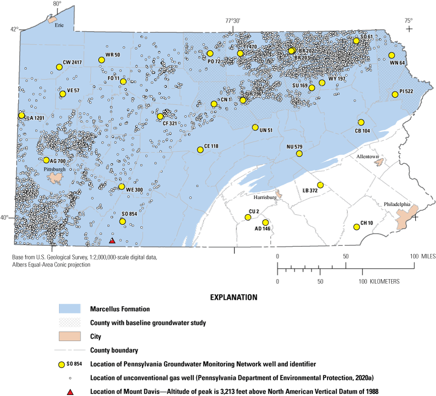
Locations of the 28 sampled wells within the Pennsylvania Groundwater Monitoring Network and associated spatial features including major metropolitan areas, counties with previous baseline groundwater quality studies, and locations of unconventional gas wells in Marcellus Shale.
Land use varies widely across the State, with development largely concentrated in the south. Forest lands in the State total 16.9 million acres (57 percent) and include State and Federally managed forests and parks in addition to private land holdings; the acreage of forested lands in the State have been relatively stable in the years following 1965 (Wildmann, 2016). Approximately 7.7 million acres (26 percent) of land are classified as agricultural, consisting of more than 59,000 farms that produce a range of products including corn, wheat, soy, apples, mushrooms, and various dairy and animal products (U.S. Department of Agriculture, 2012).
Pennsylvania has six geologically complex physiographic provinces (fig. 2) with GWMN wells located in the three largest provinces (Pennsylvania Bureau of Topographic and Geologic Survey, 2008a). The majority of the wells are located in the Appalachian Plateaus physiographic province, which is characterized by broad to narrow uplands that have been subject to glacial and fluvial erosion in varying degrees. Wells are also located in the Ridge and Valley Province, characterized by long, high parallel mountain ridges and narrow valleys, and the Piedmont Province, which is characterized by rolling hills. Both the Ridge and Valley and Piedmont provinces also contain carbonate bedrock that is characterized by karstic features. GWMN samples are collected from wells in 14 of 23 physiographic sections (subdivisions of physiographic provinces) (Pennsylvania Bureau of Topographic and Geologic Survey, 2008a,b). The majority of GWMN wells are completed in Mississippian and Pennsylvanian principle aquifers, with selected wells completed in the Valley and Ridge, Piedmont, and Blue Ridge principle aquifers (U.S. Geological Survey, 2003); several wells not located in a principle aquifer are completed in the Northern Appalachian Basin secondary hydrologic region (Belitz and others, 2018). Locations and construction information for each well in the GWMN, including the rock formation, depth, and surface elevation of the well can be found in table 1. Supplemental information for each well, including the predominant redox state as well as the minimum, median, and maximum values for dissolved oxygen, specific conductance, and pH can be found in appendix 1.
Table 1.
General information including station name, station identification number, number of samples collected, and physical characteristics of wells in the Pennsylvania Groundwater Monitoring Network.[ID, identifier; Fm, formation; NA, not applicable; --, no data]
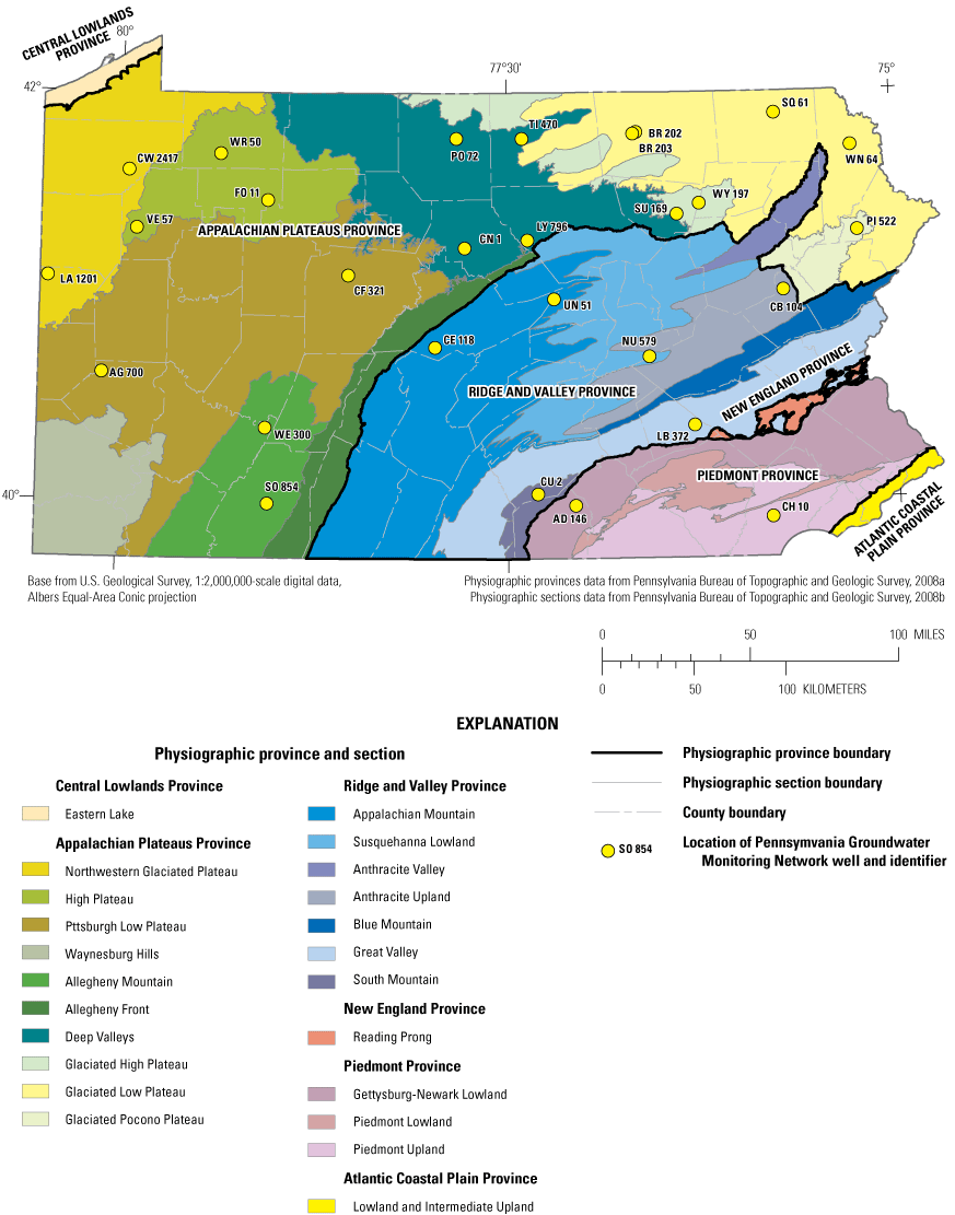
Physiographic provinces and physiographic sections of Pennsylvania and the locations of 28 sampled wells within the Pennsylvania Groundwater Monitoring Network.
The bedrock geology and associated topography of Pennsylvania (fig. 3A) are diverse, owing to historical plate tectonic activity as well as depositional and erosional events (Pennsylvania Geological Survey and Pittsburgh Geological Society, 1999; Pennsylvania Bureau of Topographic and Geologic Survey, 2001). The primary lithology (fig. 3B) of Pennsylvania’s aquifers is Ordovician to Jurassic siliciclastic rock, with a significant presence of Cambrian and Ordovician carbonate rocks in the Ridge and Valley physiographic province and Proterozoic to Cambrian crystalline rocks in the Piedmont physiographic province (Miles and Whitfield, 2001; Pennsylvania Bureau of Topographic and Geologic Survey, 1998; Soller and others, 2012). Most wells in the network are completed in bedrock formations that range from Proterozoic to Triassic in age, with the exception of wells TI 470 and WN 64, which are completed in overlying Quaternary glacial deposits that are common in the northeastern and northwestern parts of the state. Owing to an extensive history of economic materials extraction including oil, coal, and building stones in areas of the State, groundwater quality can be locally affected by the legacy of these efforts. In addition, several of the wells in the network are located within the region of Marcellus Shale gas extraction, which commenced in 2007 (Pennsylvania Department of Environmental Protection, 2020a).
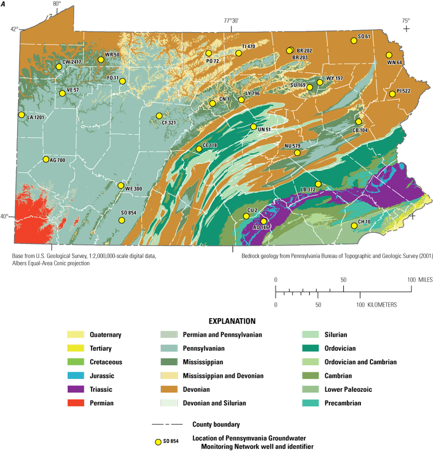
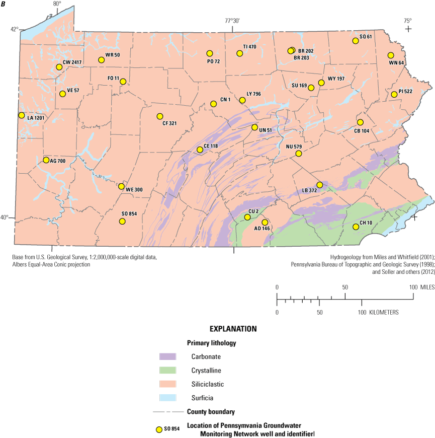
A, Age of the regional bedrock geology, and B, the primary lithology of the surficial geology of Pennsylvania and the locations of 28 wells within the Pennsylvania Groundwater Monitoring Network.
Surface water resources are dominated by three major rivers (Susquehanna, Delaware, and Ohio), which collectively drain 95 percent of the 45,000 miles of waterways in Pennsylvania. All network wells are in one of these watersheds, with the majority (57 percent) located in the Susquehanna River watershed. The degree of surface water-groundwater interaction varies with geology and topography, with particularly high connectivity in the limestone valleys found in the Ridge and Valley and Piedmont physiographic provinces. This connectivity can be of concern where chemicals from human activities, such as the disposal of wastes and the use of fertilizers and manmade organic compounds, can enter the groundwater supply. Natural lake features are limited to the northeastern and northwestern glacially influenced parts of the State; the majority of surface water bodies in the State are artificially formed or expanded reservoirs used for flood-control, water supply, and recreational purposes.
Study Methods
To characterize groundwater chemistry in aquifers, 221 groundwater quality samples were collected between 2015 and 2019 from 28 wells. Samples were analyzed for physical and chemical properties, major ions, metals and trace elements, nutrients, volatile organic compounds, radionuclides, and dissolved hydrocarbon gases including methane. All data presented in this report are available in the USGS National Water Information System (NWIS; U.S. Geological Survey, 2020). Data may also be accessed through the National Water Quality Monitoring Council’s Water Quality Portal (National Water Quality Monitoring Council, 2020), or using the dataRetrieval R package (DeCicco and Hirsch, 2021).
Selection of Sampling Locations
GWMN wells are located at existing USGS continuous monitoring stations or in locations where agreements exist between the USGS and landowners for continued access to the well. The selection of wells for the network initially focused on the northern and western parts of the State, with many being located in areas underlain by the Marcellus Shale (fig. 1). Site visits were made to several USGS continuous water-level observation wells during the fall of 2014 to evaluate site access, physical and chemical properties of the water, and the ability of the well to produce an adequate supply of water for sample collection. Subsequent additions to the GWMN have been in underrepresented regional aquifers to better reflect ambient groundwater quality in spatially diverse areas of the State; a subset of these additions are reconstructed deep test holes that were completed and sampled through cooperation with the Pennsylvania Geological Survey. Prospective wells were identified through the use of well construction records as well as through communication with personnel of various local, State, and Federal agencies. Records downloaded from NWIS and the Pennsylvania Groundwater Information System (Pennsylvania Department of Conservation and Natural Resources, 2020) are spatially joined with shapefiles of public lands in the State and validated to ensure locational accuracy and public entity ownership. Permission and communication with land operators are necessary to access and determine the existence and accessibility of the wells. Future expansion of the GWMN will continue to focus on the sampling of underrepresented aquifers in locations where agreements for long-term sampling with cooperators can be established.
Prior to being added to the GWMN, a prospective well undergoes an exploratory site visit to determine if factors such as accessibility, well integrity, and water quality would preclude the well from accurately representing the groundwater quality of the local aquifer. The integrity of candidate wells is evaluated by checking the casing for rust and the immediate vicinity for surface drainage issues; well casings also need to be above grade and have the ability to be secured to protect submersible pumps, tubing, and instrumentation inside the well. Each candidate well is pumped to examine physical and chemical water-quality properties as well as to determine whether the well is able to produce an adequate supply of water for sample collection. Physical and chemical properties are monitored during pumping of three borehole volumes to determine if stabilization of field parameters is possible (U.S. Geological Survey, variously dated). If the well is considered to be a good candidate for the GWMN, a dedicated Grundfos RediFlo 2 pump and precleaned, inert Teflon tubing is installed for future sampling events.
Collection and Analysis of Samples
A total of 221 groundwater quality samples were collected from 28 well sites between 2015 and 2019 following standard USGS methods and protocols outlined in the USGS National Field Manual (NFM; U.S. Geological Survey, variously dated). The number of samples at a specific site range from 1 to 12 depending on when the well was added to the GWMN (table 1). Samples are collected at each well twice a year, during times when water table levels generally are at or near their highest (April and May) and lowest (October and November) (fig. 4). Most samples were collected using dedicated in-place Grundfos RediFlo2 pumps and tubing to reduce the chance of cross-contamination between wells. Samples from wells BR 202 and BR 203, which are in active use, were collected from a spigot that is attached to plumbing from the well. The plumbing for these two wells was inspected prior to the initial sampling event to determine that water was untreated prior to sample collection. Static water level measurements were performed prior to the onset of pumping to determine the volume of water in the well (Cunningham and Schalk, 2011). Samples were collected for analysis following either (1) the removal of three borehole volumes of water from the well, or (2) the stabilization of field parameters to recommended ranges over the course of at least five consecutive measurements in accordance with USGS NFM guidelines (U.S. Geological Survey, variously dated). Field parameters measured during the sample collection process while pumping include air temperature, water temperature, dissolved oxygen, pH, specific conductance, turbidity, alkalinity, and water level. Flow rate was monitored using the volumetric bucket and watch method. Alkalinity was measured the day of sampling, with sample titrations occurring at the lab or in a hotel. The purging time of wells ranged from 30 minutes (0.5 hours) to more than 180 minutes (3+ hours), depending on the static volume of water and specific capacity of the well.
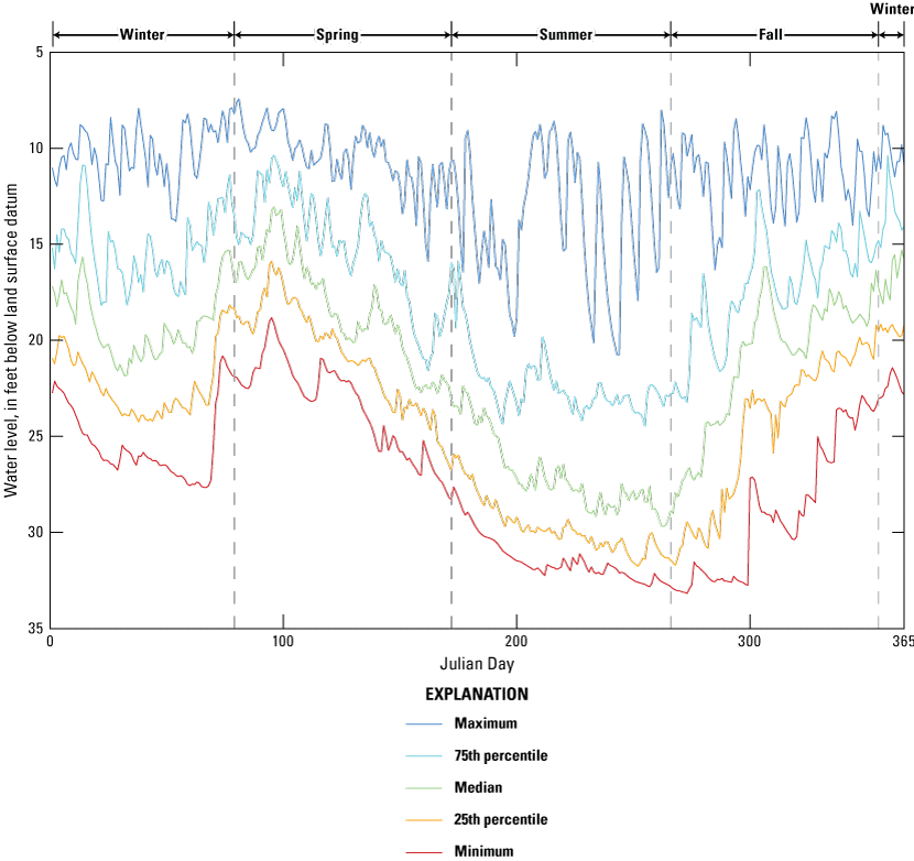
Water level daily values, 2000–19, from PO 72 Potter County observation well, displaying daily average minimum, 25th percentile, median, 75th percentile, and maximum values.
Samples were processed in the following order and manner, as recommended by the USGS NFM (U.S. Geological Survey, variously dated).
-
1. A 0.45µm (micrometer) pore filter is rinsed with 2 liters of deionized water and a plastic sampling chamber is set up to reduce atmospheric contamination of samples as recommended in the USGS NFM (U.S. Geological Survey, variously dated).
-
2. Unpreserved dissolved samples were collected for physical properties and general chemistry (pH, alkalinity, specific conductance).
-
3. Dissolved nutrients were collected and preserved with sulfuric acid, followed by dissolved metals, and dissolved organic compounds that are preserved with nitric acid.
-
4. Alkalinity samples were collected and placed on ice for titration after the site visit.
-
5. After replacing the sampling chamber, unfiltered samples were collected for general chemistry, metals (preserved with nitric acid), nutrients and total organic compounds (preserved with sulfuric acid), and cyanide (preserved with sodium hydroxide).
Throughout the course of the project, the reporting limits have changed for several constituents, mostly trace elements. This has largely consisted of increasing reporting limits (less sensitive detection levels), leading to reported values of some chemical concentrations measured from earlier samples that are less than later reporting limits. To account for changing reporting limits, each constituent was censored to the highest-available reporting limit, with all values below that level being up-censored to that reporting limit. Filtered constituents containing the most up-censored values include lead (82 percent of samples censored to the highest reporting limit), mercury (73 percent), selenium (71 percent), and antimony (67 percent). Unfiltered constituents containing the most up-censored values include silver (94 percent), orthophosphate (77 percent), mercury (70 percent), and beryllium (65 percent). To ensure consistent statistical analysis, values below the highest lab-established reporting limit for a given constituent have been up-censored to the highest reporting limit; a list of parameters with up-censored values is presented in table 2. For example, the censoring limit for both filtered and total iron was raised by the PaDEP laboratory from 8 µg/L to 18 µg/L prior to the fall 2018 sampling season. As a result of this change, 14 measured concentrations for filtered iron and 8 measured concentrations for total iron were initially reported below 18 µg/L but have been up-censored to 18 µg/L.
Table 2.
Counts and percentages of censored constituent values following up-censoring to account for changes to Pennsylvania Department of Environmental Protection Bureau of Laboratories reporting limits.[µg/L, micrograms per liter; mg/L, milligrams per liter; P, phosphorus]
Quality Assurance and Quality Control
For quality control (QC), an equipment blank was collected using a randomly selected submersible pump and tubing section prior to installation to evaluate the potential effects of the sampling apparatus (sampling pumps, tubes, and filters) on the water chemistry results. At each sampling site, pesticide-grade blank water with a deionized (DI)-water purged filter was processed as the equipment blank for dissolved organic compounds analysis. With few exceptions, these blanks registered constituent concentrations below reporting limits. Additionally, replicate samples were collected at several wells during the course of the project, including at SO 854 during the first sampling event at that well during the fall 2018 sampling season and FO 11 and SQ 61 during the spring 2019 sampling season. Duplicate pairs of filtered or unfiltered samples were collected sequentially (standard sample followed by replicate sample). Results from replicate samples indicate reproducibility was within 5 percent for most major ions and trace elements at concentrations that were greater than two times the reporting limit and within 20 percent for samples that were less than two times of the reporting limit. For the replicate samples collected from FO 11, there was a 14.3 percent difference between environmental (6,600 micrograms per liter [µg/L]) and replicate (7,700 µg/L) results for total iron and a 45.6 percent difference between environmental (2.65 µg/L) and replicate (1.44 µg/L) results for molybdenum. For the replicate samples collected from SO 854, there was a 44.5 percent difference between environmental (17.98 milligrams per liter [mg/L]) and replicate (9.97 mg/L) results for chloride and a 9.3 percent difference between environmental (2.83 mg/L) and replicate (2.59 mg/L) results for calcium.
For quality assurance (QA), intrasample characteristics of inorganic chemical analyses were evaluated using standard procedures described by Hem (1985). Evaluations of accuracy and precision included comparing field- and laboratory-measured values of pH, specific conductance, and alkalinity, as well as comparing concentrations of the filtered (dissolved) and unfiltered (total) constituents. Comparisons of filtered and unfiltered samples were generally consistent, with unfiltered samples having higher or equal concentrations than associated filtered samples except for parameters including iron, manganese, and arsenic in select samples.
Additional QA/QC checks involved comparisons of (1) the computed cation and anion equivalents concentrations and the corresponding ionic charge balance, (2) the ratios of cation or anion equivalents to measured specific conductance (SC), (3) the measured residue on evaporation (ROE) at 180 degrees Celsius (°C) to the computed total dissolved solids (TDS) as the sum of major ion concentrations, and (4) the measured SC to the computed SC. The ionic charge balance and computed SC were estimated with PHREEQC (Parkhurst and Appelo, 2013) after accounting for aqueous speciation. In general, ionic charge balance was improved using the laboratory-measured alkalinity to a fixed endpoint pH instead of the field titration with inflection point, which typically was lower than the laboratory value. Computed charge balances were within ±10 percent for 208 (94.1 percent) samples (when using laboratory-measured alkalinity). The measured and computed dissolved solids and the measured and computed SC using the laboratory alkalinity were in close agreement (fig. 5), with a few exceptions. In several cases, the computed TDS or SC was less than the measured value, which resulted in some cases because of missing concentration values for major anions (SO4, Cl). Otherwise, greater values for the measured ROE than the computed TDS could be explained by water retention in the evaporated sample (for example, Ca SO4·2H2O) instead of complete dehydration.
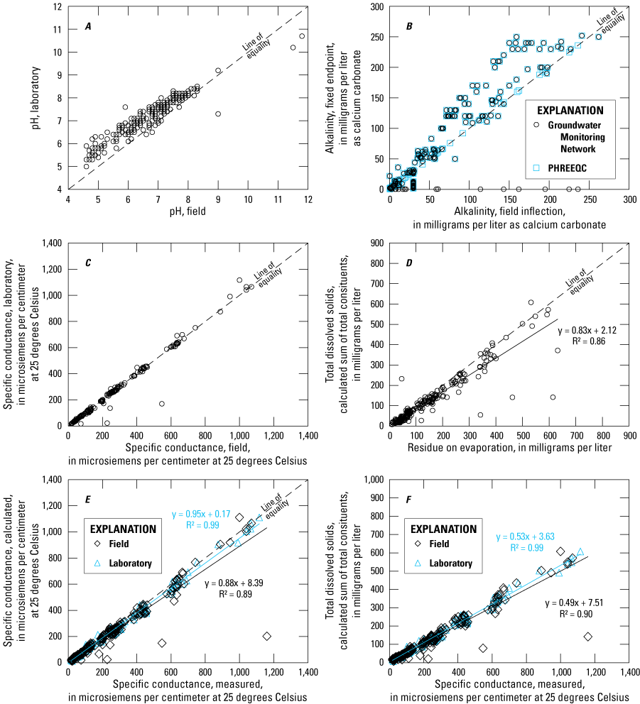
Comparison of field, laboratory, and (or) computed values of pH and specific conductance (SC) and total dissolved solids (TDS) for 221 samples collected from 28 wells within the Pennsylvania Groundwater Monitoring Network, 2015–19. A, Field and laboratory measured pH; B, field and laboratory measured alkalinity; C, field or laboratory measured SC and calculated SC on the basis of ionic conductivities; D, measured TDS (as residue on evaporation at 180 °C) and calculated TDS as the sum of dissolved constituent concentrations; E, measured and computed SC; and F, field or laboratory measured SC and calculated TDS on the basis of dissolved constituent concentrations.
Climate and Landscape Characteristics
Data analysis of samples within the GWMN focuses on several categorical variables, including geology and physiography, land use, topographic position, and drought severity. These variables were used to subset the samples into various groups for targeted analysis that were used to determine if common traits were shared among wells within the GWMN. Spatial data was accessed through the Pennsylvania Bureau of Topographic and Geologic Survey and accessed from the Pennsylvania Spatial Data Access (PASDA) database (Pennsylvania Spatial Data Access, 2020). The geologic formation, physiographic province, and physiographic region where each well in the GWMN is completed in were determined using spatial data digitized from the 1980 Geologic Map of Pennsylvania (Berg and Dodge, 1981).
Land use was calculated for a boundary radius of 1,000 meters (m) around each well location. Land use data were gathered from the 2011 National Land Cover Database (U.S. Geological Survey, 2014) and clipped to each buffer around each well in ArcGIS. The percentages of land cover in each buffer area were determined for the following categories: forested, cultivated, shrub/herbaceous, water/wetlands, and developed. Generally, wells in the GWMN are in areas that represent little or low-grade land usage and development. A description of land use around each well can be seen in figure 6. Twenty-three of the 28 wells that are currently established in the GWMN are surrounded by 50 percent or more forested land and 7 of the wells are located in areas where greater than 25 percent of land is cultivated. Only 4 of the wells are located in areas with greater than 10 percent of land covered by water or wetlands, and only one well (LB 372) is located in a predominantly developed area.
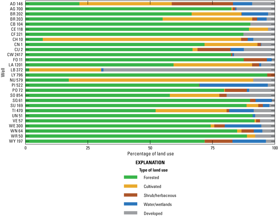
Land use within 1,000 meters of each sampled well within the Pennsylvania Groundwater Monitoring Network. Land use data from the 2011 National Land Cover Database (U.S. Geological Survey, 2014).
The topographic position for each well in the GWMN was determined using a digital elevation model (DEM) raster dataset to evaluate peaks, valleys, and slopes on the landscape (Jenness, 2006). The DEM was converted to a raster dataset with 10-m resolution that evaluated the slope of each point in the file. To access slope values for each well, a spatial join was performed to match each well with the closest cell in the raster dataset. Topographic position was categorized into three general categories (valley, slope, and ridge) based on examination of regional slope and elevation patterns.
The Palmer Drought Severity Index (PDSI) estimates the relative dryness of a location using temperature, soil moisture, and precipitation data (Palmer, 1965; Dai and others, 2019). PDSI is a tool that can be used to measure periods of long-term wetness or drought over a regional space; limitations of PDSI include the limited spatial areas that were used to define the index, the absence of a way to handle frozen ground surfaces, and the arbitrary designation of parameters such as depth of soil where moisture is available to be mobilized via evapotranspiration (Alley, 1984). Values for PDSI typically range between –4 and 4 (although higher and lower values are possible under exceptionally wet or dry conditions), with negative numbers indicating mild (–1 > PDSI > –2), moderate (–2 > PDSI > –3), severe (–3 > PDSI > –4), or extreme (PDSI < –4) drought conditions, and positive values signifying increasingly wet conditions. Each individual sample collected in the GWMN was assigned the corresponding PDSI value for the location of the well when the sample was collected. Palmer Drought Severity Index values are computed on a 4-kilometer grid and were accessed using the ClimateR R package; values were collected for samples collected between 2015 and 2018 from each grid cell that a well was located in (Johnson, 2020). Ten unique variables were created; one was the PDSI value at the well during the month of the sampling event, and the other nine variables are PDSI values from each of the preceding nine months. Previous PDSI values were incorporated owing to the delayed response often seen in groundwater as precipitation rates change.
Data Analysis Methods
All analysis was completed using R, an open-source environment for statistical computing (R Core Team, 2019). An assortment of geospatial and geochemical methods were used in this report to characterize water quality on a network scale, to distinguish differences in water chemistry between wells within the GWMN, and to identify factors that may be responsible for changes in water chemistry over the course of multiple sampling seasons. Bivariate plots were produced to illustrate relations between various parameters and pH, specific conductance, and dissolved oxygen. Major ion data are presented in Piper diagrams (Piper, 1944) to characterize geochemical differences among wells within the GWMN and possible water chemistry processes that drive constituent concentrations. The Piper diagram was produced using the smwrGraphs package in R (Lorenz and Diekoff, 2017). Reduction/oxidation (redox) processes were identified based on the concentrations of dissolved oxygen, nitrate, sulfate, iron, and manganese (McMahon and Chapelle, 2008). Boxplots of selected constituents were grouped by variables including pH, specific conductance, redox state, physiographic province, major aquifer type, topographic position index, and season (appendix 3).
The summary statistics of sampled constituents were computed using a dataset that had censored values removed to capture the distribution of values with detectable concentrations at the highest reporting limit of a particular constituent; these results are presented alongside EPA drinking water standards including maximum contaminant levels (MCLs; U.S. Environmental Protection Agency, 2020a), secondary maximum contaminant levels (SMCLs; U.S. Environmental Protection Agency, 2020b), and health advisory levels (HALs; U.S. Environmental Protection Agency, 2018a). In addition, advisory levels for methane from PaDEP and U.S. Department of Interior are considered (Eltschlager and others, 2001; Pennsylvania Department of Health, 2019). The number and percentage of detectable concentration results is also noted in tables of summary statistics. Medians presented in summary tables are calculated from the median values of each well to account for differing amounts of samples from each location. For most analyses, nonparametric methods were used to account for non-normal data distributions and the presence of data censored at the highest common reporting limit that is common in environmental sampling (Helsel and others, 2020). All data was censored to the highest laboratory reporting limits used during the sampling period; in several instances, measured values were censored owing to the increase of laboratory reporting limits.
Principal components analysis (PCA) and hierarchical clustering were computed with the FactoMineR package (Lê S and Husson, 2008) and used to evaluate multivariate correlations among dissolved constituents and field parameters including pH, specific conductance, and dissolved oxygen. Results of the PCA were used to identify geochemical processes or variables that explain patterns of constituent distributions and associations (Joreskog and others, 1976; Thyne and others, 2004). Data used in PCA calculations were ranked to standardize variable contributions and values censored at the highest common reporting limits were used in situations where samples had constituent readings below reporting limits. A total of 200 out of 221 groundwater samples (90.5 percent) contained a complete set of variables for the PCA analysis. Parameters included in the PCA consist of major ions and selected trace elements and field parameters. Redundant constituents, such as total concentrations of elements, laboratory-measured field parameters, and autocorrelated measurements such as hardness were not included in the PCA. Only principal components (PCs) with an Eigenvector greater than unity were retained for analysis (Joreskog and others, 1976; Thyne and others, 2004). Unity, also known as the Kaiser criterion, is equal to 1 and is the level at which a PC extracts at least as much information as any singular variable does in the analysis (Kaiser, 1960). Loadings from the PCA were optimized by rotation in order to maximize the differences between PCs. Hierarchical clustering is a classification method that allows inferences to be made regarding the similarity or dissimilarity between individual members of a group and was performed using PCA results to display spatial patterns of wells that have similar water chemistry. Clustering was performed using Ward’s method, which is an agglomerative process that groups similar samples into clusters (Ward, 1963). Hierarchical clustering results are presented graphically using median concentration values from each well for visual clarity. To aid in the broader interpretation of water quality data, scores for PCs were evaluated through correlation with additional variables that were not included in the PCA, such as land surface elevation, PDSI values (both at sample time and lagged to account for extended influences of precipitation), and other minor constituents that were employed in the model. PCA results were also analyzed through the use of hierarchical clustering to denote subsets of wells that experience similar chemical processes to further explain the development of components from the PCA.
An analysis of differences between total and dissolved constituents was performed to evaluate the sensitivity of the laboratory’s instrumentation with regard to whole and filtered samples. Each sample set consists of filtered and unfiltered samples for major ions, trace elements, and nutrients. The nonparametric Wilcoxon rank-sum test was performed using the exactRankTests R package (Hothorn and Hornik, 2019). Within each rank sum test, filtered and unfiltered samples were paired to ensure that evaluations were being performed on the two variables for each sample collected; values that were unable to be paired were dropped from analysis. The exact Wilcoxon rank-sum test was employed owing to its robustness when evaluating non-normal distributions of data and because it uses the Streitber-Röhmel shift algorithm to handle ties within the dataset; this is particularly useful when analyzing environmental data, when many of the values in a dataset are either at or just above the reporting limit (Streitberg and Röhmel, 1986).
Wilcoxon rank-sum tests were also used to evaluate differences between samples that were collected in times of greater than average precipitation (PDSI > 0) and times of less than average precipitation (PDSI < 0). Rank-sum tests were performed using the PDSI values from the month that a particular well was sampled, as well as values lagged from 1 to 9 months prior to the sample to capture differences that may occur in long-term groundwater movement. Constituents, including calcium, magnesium, sodium, chloride, and lithium were evaluated for differences between positive and negative PDSI phases. Differences that may be caused by the changes in sampling seasons (such as spring and fall) were evaluated on both a network and by individual well using Wilcoxon rank-sum tests. Only constituents with more than 50 percent of recorded values above the reporting limit were included in this analysis. For the analysis of individual wells, only wells that had at least four spring and four fall samples were included to account for anomalously high or low readings that may be present. Temporal trends in constituent values among these wells were also evaluated using the Mann-Kendall Trend test; this test was performed using the trend R package (Pohlert, 2020). Median concentrations of constituents were calculated for each sampling season to determine if general GWMN trends are increasing or decreasing over time.
Status of Groundwater Quality Constituents
Results of the 221 groundwater quality samples are presented in the context of drinking-water standards and discussed below. Three standard criteria—MCLs, SMCLs, and HALs—are considered (U.S. Environmental Protection Agency, 2020a, b). These standards are only enforceable for public water supplies but are considered guidelines for all private water supplies. MCLs are set to reflect levels at which a constituent may begin to affect human health, and SMCLs are set to reflect levels at which a constituent may begin to affect the aesthetic quality of the water. HALs are non-enforceable guidance for constituents that may affect human health. Results for unfiltered samples are typically evaluated for potential human health effects because both dissolved and suspended constituents in whole-water samples contribute to drinking-water exposure; however, unfiltered samples introduce variability associated with sampling procedures, so they are not as readily interpreted as filtered samples with respect to the geochemical environment. Thus, some element concentrations are reported for both filtered and unfiltered samples; differences between filtered and unfiltered constituents are displayed in table 3. For each sampling event at a well, a suite of constituents was analyzed; they are grouped herein as physical and chemical properties, major ions, metals and trace elements, nutrients, and dissolved organic compounds. Summary statistics are presented for each analyte class and are presented in tables 4–9. Information about the units for each constituent are included in those tables; concentrations are typically reported in mg/L or µg/L, with radiochemical concentrations reported in picocuries per liter (pCi/L). In addition, during the first sampling event at each well, a wider spectrum of sampling was completed. Summary statistics for analyses including VOCs, dissolved hydrocarbon gases, radiological elements, and dissolved hydrocarbons including methane are presented; repeated sampling of these parameters was generally not completed.
Table 3.
Results of Wilcoxon rank-sum tests that compare the paired filtered and unfiltered samples for selected constituents for 221 samples collected from 28 wells within the Pennsylvania Groundwater Monitoring Network, 2015–19.[µg/L, micrograms per liter; mg/L, milligrams per liter; N, nitrogen]
Comparison of Total and Dissolved Concentrations
Filtered and unfiltered samples were collected for analysis of major ions and trace elements to evaluate differences and determine if both filtered and unfiltered samples are necessary. Filtering samples removes suspended particles greater than 0.45 microns, along with any chemicals sorbed onto those particles. Conversely, suspended particles and associated chemicals sorbed onto them are not removed from unfiltered samples.
Filtering groundwater samples is a standardized procedure that reduces variability associated with the disturbance of a well or aquifer by sampling and is considered more representative of ambient conditions (U.S. Geological Survey, variously dated). However, the suspended particles may dissolve in the human digestive tract once consumed. Thus, unfiltered samples are important for characterizing drinking water because private domestic supplies may not have filtration and (or) disinfection systems.
The differences between filtered and unfiltered constituent concentrations in groundwater arise as a result of varying levels of solubility; some constituents readily dissolve in water, whereas others have more restricted parameters for dissolution, leading to expected higher concentration levels in unfiltered samples than in their filtered counterparts. To determine if there are significant differences between the total and filtered samples, a Wilcoxon rank-sum test was used to compare the values collected for each constituent. Results of Wilcoxon rank-sum tests are presented in table 3. Constituents with a significant difference (P < 0.05) between filtered and unfiltered samples include silica, barium, iron, manganese, and arsenic—all trace elements that are commonly present in natural waters as suspended particles owing to low solubilities (Hem, 1985). Elements that do not have a large difference between filtered and unfiltered samples include chloride, calcium, and magnesium, which are typically found in solution. Dissolved and total concentrations differed significantly for phosphorus but not nitrate; this is a result of the low solubility of most phosphorus-containing compounds (Hem, 1985).
Concentrations of constituents with higher differences between filtered and total concentrations, which included arsenic, iron, and manganese, are shown in cumulative distribution frequency plots (fig. 7). Only paired observations were used for this analysis to ensure that cumulative frequencies of measurements were consistent for filtered and total samples. The differences between filtered and total manganese concentrations were typically found at concentrations below 100 µg/L, whereas both total iron and arsenic concentrations were consistently higher than their filtered concentration counterparts across the entire range of measurements. When laboratory reporting limits are set for constituents that contain low-solubility oxide compounds, the detection limits for filtered samples are effectively lower and analyses are more sensitive than those for whole water samples because of the removal of suspended particles that occurs during filtration. At lower concentrations, the differences in concentration between filtered and total samples may fall within the precision range of the measurement; for wells with higher concentrations where suspended particles are the dominant source of low-solubility metals, differences of an order of magnitude or greater may be recorded. In limited cases, the filtered concentrations of these metals (particularly manganese at wells FO 11, LA 1201, and WN 64 and arsenic at wells AD 146, AG 700, CF 321, CN 1, CU 2, FO 11, LA 1201, LB 372, NU 579, SO 854, and SQ 61) are slightly higher than total concentrations and are likely a result of the majority of the metal being in solution as well as a sensitivity to reducing conditions. Only 14 of 221 samples (6 percent) contained total lead levels that were higher than the maximum filtered lead value recorded; 3 of these samples were collected from well VE 57. Thirteen (46.4 percent) GWMN wells in the network do not have measurable levels of filtered iron, 15 (53.6 percent) wells do not have measurable levels of filtered arsenic, and 8 wells (28.6 percent) do not have measurable levels of filtered manganese samples. This suggests that the low solubility of these metals leads to filtered samples being more sensitive to detection and therefore more commonly reported as a nondetect when concentrations of unfiltered samples are at the low end of the detection range.
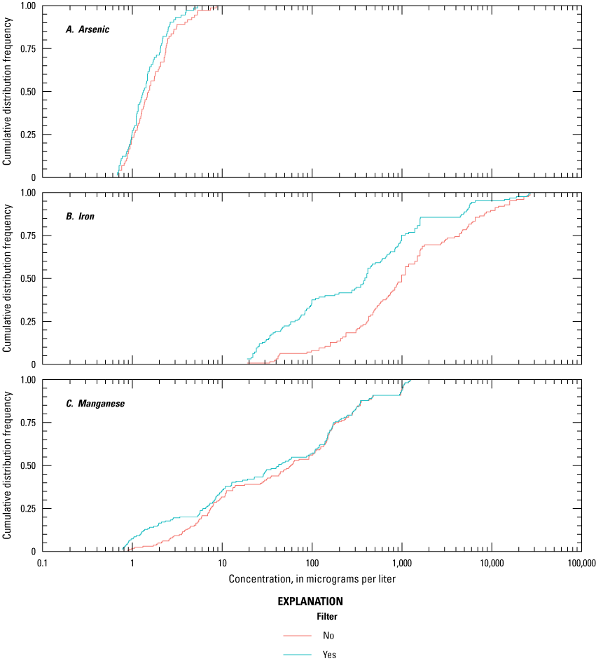
Cumulative distribution frequency plots of total and dissolved arsenic, iron, and manganese using paired samples from Pennsylvania Groundwater Monitoring Network samples, 2015–19.
Physical and Chemical Properties
Physical and chemical properties that are measured during well sampling include water temperature, dissolved oxygen, pH, specific conductance, turbidity, and alkalinity. Summary statistics for these physical and chemical properties and associated measures such as the air temperature and barometric pressure are given in table 4.
Table 4.
Minimum, median, and maximum values of physical and chemical properties for 221 water samples collected from 28 wells within the Pennsylvania Groundwater Monitoring Network, 2015–19.[°C, degrees Celsius, µS/cm, microsiemens per centimeter; mg/L, milligrams per liter; mV, millivolts; NTRU, Nephelometric Turbidity Ratio Units; %, percent; CaCO3, calcium carbonate; USGS, U.S. Geological Survey; NFM, National Field Manual; SM, Standard Methods for the Examination of Water and Wastewater; EPA, U.S. Environmental Protection Agency; MCL, maximum contaminant level; SMCL, secondary maximum contaminant; level,wu, undissolved water sample; wu,recov, undissolved water sample, recovered; dissolved, dissolved water sample; fld, field measurement; --, no MCL or SMCL established]
Water temperatures for wells sampled in this study ranged from 7.0 to 13.3 °C, with a median of 10.1 °C (table 4). Water temperatures were generally lower than air temperatures in the spring sampling seasons and higher than air temperatures in the fall sampling seasons, reflecting a groundwater environment that is generally cool and stable.
The concentrations of dissolved oxygen (DO) ranged from 0 to 13.9 mg/L, with a median value of 2.85 mg/L. Although some wells, including LB 372, PI 522, WE 300, and WN 64, exhibited a range of DO concentrations, most other wells in the network consistently display anoxic or oxic conditions (appendix 1). Most samples had DO values less than 100 percent of saturation, which is the value at equilibrium with the atmosphere, indicating that the waters being sampled were out of contact with the atmosphere (Gross and Cravotta, 2017; U.S. Geological Survey, 2018). The relation between DO concentration and pH (fig. 8) in the network is complex; samples with pH below 5.5 were consistently oxic (DO > 2.0 mg/L), whereas wells located in carbonate settings (LB 372, CE 118) had both high DO and pH. Several wells in the GWMN consistently display anoxic conditions, with DO levels lower than 0.5 mg/L. These wells (SO 854, CF 321, FO 11, WR 50, WY 197, CW 2417, SQ 61, and BR 202) also exhibited a range of pH values from 5.5 to 8.4. Low DO concentrations are an indicator of chemical processes that consume oxygen, such as the decomposition of organic carbon, and may be associated with chemically reducing conditions that promote the release of constituents from bedrock and substrate including iron, manganese, and other metals (Clune and Cravotta, 2019). Of the 204 samples with DO results, 65 (31.6 percent) were classified as anoxic (≤0.5 mg/L), 44 (21.9 percent) were classified as mixed (>0.5 mg/L and ≤2.0 mg/L), and 95 (46.5 percent) were classified as oxic (>2.0 mg/L). Of the 65 samples classified as anoxic, 46 (70.8 percent) had chemical characteristics favorable for reduction of Mn(IV) and (or) Fe(III) (McMahon and Chapelle, 2008); however, none of the results from these samples were associated with the strongly reducing conditions necessary for methanogenesis (McMahon and Chapelle, 2008; Clune and Cravotta, 2019). Only one well, SQ 61, consistently displayed conditions favorable for Mn(IV) reduction (appendix 1); other anoxic wells contained conditions favorable for more than one redox process. Reducing conditions were noted in all or most samples collected from wells AG 700, CF 321, FO 11, LA 1201, SO 854, SQ 61, WR 50, and WY 197.
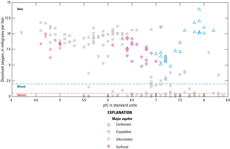
Relation between pH and dissolved oxygen (DO) concentrations in Pennsylvania Groundwater Monitoring Network samples, 2015−19. Anoxic water contains <0.5 milligrams per liter (mg/L) of DO, mixed water contains ≥0.5 mg/L but <2 mg/L of DO, and oxic water contains ≥2 mg/L of DO.
The pH of water is a measure related to acidity and the potential of water to be corrosive and leach metals from pipes and plumbing (Belitz and others, 2016; Gross and Cravotta, 2017). The pH scale is logarithmic and runs from 0 to 14, with 7 being neutral. Values of pH below 6.5 are generally considered acidic, whereas values above 7.5 are alkaline. pH values between 6.5 and 7.5 are considered near neutral. pH generally increases with the amount of time that water is underground and with the distance that it travels from the point of infiltration, mobilizing naturally occurring contaminants in the process of cation exchange. The pH results for this study range from 4.2 to 11.8, with a median of 6.85; the majority of wells exhibited a pH range of less than one standard unit (appendix 1). Ninety-two of the samples collected (42 percent) fall outside of the EPA SMCL range of 6.5 to 8.5. Of the samples that are outside of the range of 6.5–8.5, only 4 (4.3 percent) were above the upper end of the range; all of the samples with pH greater than 8.5 were collected at well SU 169. Well SU 169 was reconstructed in 2017 to target the most productive fracture in the hole; loose grout containing bentonite clay from the reconstruction may be the primary cause of higher than expected pH values. Sampling in fall 2019 revealed that a higher pumping rate and a longer pumping duration was necessary to clear the loose grout from the well; the measured pH from this visit was 7.2. The 88 samples (95.7 percent) with pH less than 6.5 exhibited low conductivity and high DO.
Alkalinity is a measure of water’s ability to neutralize acid and is commonly the result of carbonate and bicarbonate ions in solution (Hem, 1985). Alkalinity is related to the pH of water and samples, with higher concentrations of alkalinity in samples with pH greater than 6.5. Alkalinity as calcium carbonate ranged from 0.30 to 262.2 mg/L, with a median concentration of 63.1 mg/L. Wells finished in limestone aquifers generally had the highest measured alkalinities, whereas wells in sandstone aquifers had the lowest measured alkalinities.
Water hardness, which is computed as the sum of dissolved calcium multiplied by a factor of 2.5 plus dissolved magnesium multiplied by a factor of 4.1, ranged from 5.57 to 326 mg/L as calcium carbonate (CaCO3; table 3). Hardness is associated with the dissolution of calcium and magnesium bearing minerals that are common in limestone and other calcareous sedimentary rocks (Hem, 1985). Using a common hardness classification system described in Dufor and Becker (1964), 114 (52.1 percent) of the water samples were classified as soft (hardness <60 mg/L), 39 (18.2 percent) samples were classified as moderately hard (hardness of 61 to 120 mg/L), 33 (15.1 percent) samples were classified as hard (hardness of 121 to 180 mg/L), and 32 (14.6 percent) samples were classified as very hard (hardness >180 mg/L). Waters with low pH (below 6.5) were generally classified as soft water, as were samples with a pH above 8.0. Waters with a calculated hardness >60 mg/L as CaCO3 generally corresponded with pH values that ranged from 6.5 to 8.0, which is the range where bicarbonate is the predominant ionic contributor to alkalinity in solution (fig. 9). Carbonate aquifers tend to provide the highest values for hardness (appendix 3). Thus, alkalinity and hardness tend to be correlated.
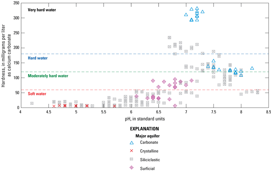
Relation between pH and total hardness in Pennsylvania Groundwater Monitoring Network samples, 2015−19. Soft water contains hardness ≤60 mg/L, moderately hard water contains hardness from >61 mg/L to ≤120 mg/L, hard water contains hardness from >121 mg/L to ≤180 mg/L, and very hard water contains hardness >180 mg/L.
Specific conductance (SC), expressed in units of microsiemens per centimeter (µS/cm), is a gross measure of the ability of ions in water to conduct an electrical current (Hem, 1985). Higher values of SC are associated with higher concentrations of dissolved solids (figs. 5 and 10). Field measurements of SC ranged from 18 to 1,160 µS/cm, with a median value of 203.3 µS/cm; the median difference between minimum and maximum conductivities for all wells in the GWMN was 25.5 µS/cm (appendix 1). Laboratory measurements of SC are equivalent to field SC values with few exceptions; in these cases, laboratory SC values are higher than those measured in the field and may have been affected by the presence of microbubbles in water that adhered to the probe surface. Higher conductivities were positively correlated with higher concentrations of several constituents including calcium, magnesium, sodium, chloride, potassium, and fluoride (Conlon, 2021).
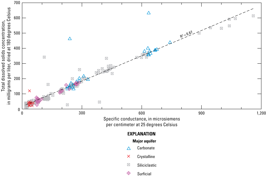
Relation between field-measured specific conductance and total dissolved solids concentrations in Pennsylvania Groundwater Monitoring Network samples, 2015–19. Dashed line represents linear relation (R2 = 0.87) between measured specific conductance and laboratory measured dissolved solids.
Turbidity is a measure of the number of solid particles that are suspended in water that block the transmission of light through a sample. Turbidity is expressed in nephelometric turbidity ratio units (NTRU), which quantifies the degree to which light is scattered by the suspended particles in the sample; higher NTRU readings indicate a more turbid sample. Turbidity concentrations in 164 samples range from 0.1 to 340 NTRU, with a median concentration of 1.85 NTRU. In general, higher NTRU concentrations are associated with samples that have elevated levels of constituents that are commonly suspended in water. Fifty-nine samples (36.0 percent) from 6 wells (21 percent of wells) had a turbidity value greater than the EPA MCL of 5 NTRU for public water systems; this includes all or most samples collected from wells CU2, UN 51, FO 11, WN 64, TI 470, and SQ 61 (U.S. Environmental Protection Agency, 2020a).
Major Ions
Major ions (table 5) constitute the majority of naturally present solutes in groundwater and are broadly characterized as those common elements or compounds with dissolved concentrations greater than 1 mg/L in natural waters. They originate from soil and rock as a result of the dissolution of carbonate, silicate, and oxide minerals, as well as from ions in precipitation. Anthropogenic sources such as de-icing salts may also contribute to the presence of major ions. Major ion concentrations are directly related to cumulative measures of ionic strength such as salinity, dissolved solids, and specific conductance; general increases in constituent values occur with progressive evaporation or dissolution of minerals (Hem, 1985).
Table 5.
Minimum, median, and maximum concentrations of major ions for 221 samples collected from 28 wells within the Pennsylvania groundwater Monitoring Network, 2015–19.[mg/L, milligrams per liter; °C, degrees Celsius; EPA, U.S. Environmental Protection Agency; MCL, maximum contaminant level; SMCL, secondary maximum contaminant level; HAL, health advisory level; total, total water sample; total, recoverable, total water sample, recovered; dissolved, dissolved water sample; --, no MCL or SMCL established; * indicates a HAL, these are not included in counting samples that exceed a standard]
Major ions are divided into two balanced groups consisting of positively charged cations (sodium, potassium, calcium, and magnesium) and negatively charged anions (chloride, nitrate, sulfate, fluoride, and bicarbonate). Additionally, silica is a major ion that is commonly uncharged, contributing to dissolved solids but not to specific conductance. Both filtered and unfiltered samples were analyzed to represent dissolved and total concentrations of major ions, respectively (table 4); however, only the dissolved concentrations are considered for milliequivalent units used for ion balance and evaluation of water types.
Total dissolved solids (TDS) is a measurement of the total amount of remaining solids following the evaporation of a water sample. TDS concentrations ranged from 10 to 632 mg/L, with a median concentration of 124.5 mg/L. Of 220 samples analyzed for TDS, only 7 (3.2 percent) from 2 wells exceeded the EPA SMCL of 500 mg/L. Six of the seven samples that exceeded 500 mg/L came from well BR 202, which also had the highest levels of dissolved sodium and chloride within the GWMN (median concentrations of 207 mg/L and 200 mg/L, respectively; table 4). High levels of sodium and chloride concentrations could be naturally occurring and increase slightly with depth in the region (Stanton and others, 2017). Dissolved concentrations of sodium and chloride plotting on the line of equality can signify concentrations from dissolution of pure sodium-chloride (NaCl) salt. However, a majority of samples (62.9 percent) have excess sodium concentrations (plotting above the line) compared to chloride, indicating that cation exchange could be an active process in many of the sampled wells. Although sodium and chloride both may be elevated across the GWMN, samples affected by cation exchange typically have molar Na:Cl ratios much greater than 1 with neutral to alkaline pH, combined with higher alkalinity and lower DO values.
Concentrations of dissolved sodium ranged from 0.38 to 239 mg/L, with a median concentration of 6.24 mg/L (table 4). Seventeen of 220 samples analyzed for dissolved sodium (5.8 percent) exceeded the EPA HAL of 20 mg/L for sodium in drinking water for people on a low-sodium diet (U.S. Environmental Protection Agency, 2003, 2018b); all of these samples were from wells AG 700, BR 202, and LB 372. The concentrations of dissolved chloride ranged from 0.28 to 200.0 mg/L, with a median concentration of 2.5 mg/L. None of the 203 samples analyzed for dissolved chloride exceeded the EPA SMCL of 250 mg/L for chloride in drinking water. The highest values for chloride in the GWMN were also found at wells AG 700, BR 202, and LB 372. A subset of wells including CW 2417, LA 1201, LY 796, SQ 61, UN 51, WR 50, and WY 197 routinely contain sodium concentrations that are more than twice as high as corresponding concentrations of chloride, indicating that cation exchange is an active process in many of the aquifers sampled by the network (Hem, 1985). These wells are highlighted in a Piper diagram (Piper, 1944), which displays the relative contributions of major ions to the total concentrations during the fall 2019 sampling season (fig. 11). The majority of samples collected are a calcium- and bicarbonate-dominant water type, especially those with excess sodium that were collected from regions underlain by siliciclastic and carbonate rocks. Samples with higher specific conductance (>500 µs/cm) had sodium-potassium dominant waters, indicating that alkali metals exceed alkaline earth metals in solution. The subset of wells that contain high sodium relative to chloride concentrations plot as calcium-magnesium/bicarbonate water types, indicating that the disparity between sodium and chloride concentrations are not the primary driver of ion contributions for those wells. The balance between anions (shades of red) and cations (shades of blue) for most wells (fig. 12) are slightly dominated by cation contributions and are driven by the prevalence of siliciclastic and carbonate rocks in many of the sampled aquifers; minor constituents including iron, manganese, strontium, and fluoride may provide important ionic contributions for some wells, but they are not included on this plot.
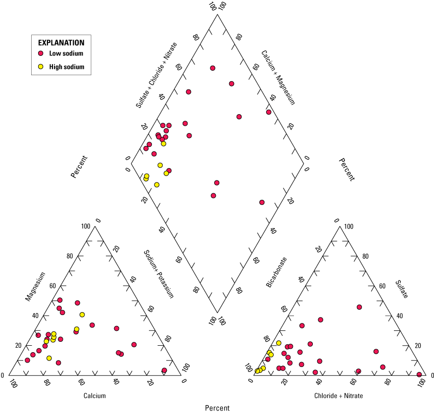
Predominant water types collected from 28 wells within the Pennsylvania Groundwater Monitoring Network during the fall 2019 sampling season. The subset of wells labeled as high sodium contain sodium in concentrations greater than two times the expected 1:1 molar ratio of sodium and chloride in pure sodium chloride salt (NaCl).
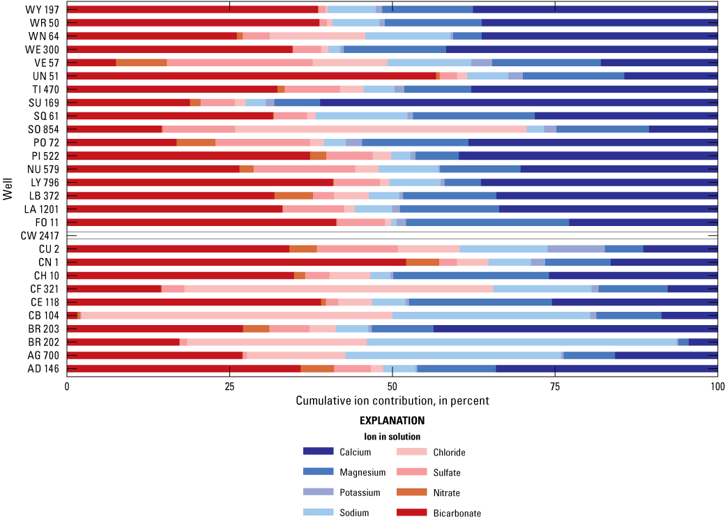
Cumulative ion contributions of samples collected from 28 wells within the Pennsylvania Groundwater Monitoring Network during the fall 2019 sampling season. Positively charged cations are represented in shades of blue and negatively charged anions are represented in shades of red.
Metals and Trace Elements
Metals and other trace elements are typically found in concentrations <1 mg/L in natural waters (Hem, 1985). Metals and trace elements that are present in groundwater can originate from soils or bedrock dissolution but may also be present in precipitation; concentrations can also be affected either directly through consumption or indirectly as a result of changes in pH and redox state caused by the presence and activity of microorganisms at depth (Lovely and Chapelle, 1995; Clune and Cravotta, 2019). Summary statistics for concentrations of total and dissolved metals and trace elements are presented in table 6. The EPA has established MCLs and SMCLs for several trace element constituents; counts of exceedances for each constituent are presented in table 5. No MCLs were exceeded, but SMCLs were exceeded for 111 samples of unfiltered (50 percent) and 70 samples of filtered (32 percent) iron, 86 samples of unfiltered (39 percent) and 79 samples of filtered (36 percent) manganese, and 45 samples of unfiltered (20 percent) and 11 samples of filtered (5 percent) aluminum. In addition, 29 samples (15.5 percent of total and 17.1 percent of dissolved samples above reporting limits, respectively) had a manganese concentration greater than the 300 µg/L HAL and health-based screen level (Norman and others, 2018; U.S. Environmental Protection Agency, 2018a).
Table 6.
Minimum, median, and maximum concentrations of metals and trace elements for 221 samples collected from 28 wells within the Pennsylvania Groundwater Monitoring Network, 2015–19.[µg/L, micrograms per liter; EPA, U.S. Environmental Protection Agency; MCL, maximum contaminant level; SMCL, secondary maximum contaminant level; total, total water sample; total, recoverable, total water sample, recovered; dissolved, dissolved water sample; NA, not applicable; --, no MCL or SMCL established]
Iron, manganese, aluminum, and copper can have undesirable effects on the odor, taste, and color of water. Iron can cause water to have a rusty color and leave a red or orange stain on laundry and plumbing materials (U.S. Environmental Protection Agency, 2020b). Total recoverable iron concentrations from 193 samples above the reporting limit ranged from 19 to 27,000 µg/L, with a median concentration of 83.5 µg/L. Wells with samples higher than the SMCL of 300 µg/L include AG 700, CF 321, CU 2, CW 2417, FO 11, LA 1201, LY 796, SO 854, WE 300, WR 50, and WY 197. Several of these wells routinely produce water that has a high enough iron content to stain the bottles that samples are collected in; the highest iron concentrations are found in wells with anoxic conditions, consistent with reducing conditions (appendix 3). Manganese at high concentrations can give water a dark black color and a bitter taste (U.S. Environmental Protection Agency, 2020b). Total recoverable concentrations of manganese in 185 samples above the reporting limit ranged from 0.72 to 1,260 µg/L, with a median concentration of 19.95 µg/L. Several wells have iron and manganese concentrations that exceed the SMCLs; of these, only one (CU 2) contains an elevated iron level along with a manganese level below 50 µg/L, and only two (WE 300 and SQ 61) contain an elevated manganese level without a corresponding iron level about the SMCL (fig. 13). The well with the highest levels of both iron and manganese was CF 321, which is completed in the Mississippian Burgoon Sandstone; this formation is noted for containing coal beds and plant fossils, which may be a source of manganese owing to its importance in the metabolic cycle of plants (Berg and others, 1980; Hem, 1985). The concentrations of both iron and manganese were negatively correlated with dissolved oxygen concentrations (fig. 14), indicating that reductive dissolution of iron and manganese oxides in bedrock may be a source of the metals in water. Other possible sources of iron and manganese include dissolution of sulfide and carbonate minerals.

Spatial distribution of iron and manganese secondary maximum contaminant level exceedances of samples collected from 28 wells within the Pennsylvania Groundwater Monitoring Network during the fall 2019 sampling season.
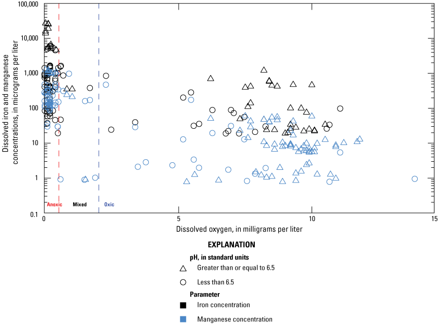
Relation between iron and manganese and dissolved oxygen (DO). Samples are split by those with low pH (≤6.5) and those with high pH (>6.5). Anoxic water contains <0.5 milligrams per liter (mg/L) of DO (below red dashed line), mixed water contains ≥0.5 mg/L but <2 mg/L of DO (between red and blue dashed line), and oxic water contains ≥2 mg/L of DO (above blue dashed line).
Dissolved copper concentrations ranged from 0.42 to 11.7 µg/L, with a median concentration of 0.66 µg/L; none of the 112 samples above the reporting limit were above the SMCL of 1 mg/L (1,000 µg/L). All the samples with >8 µg/L copper were collected from well BR 203; plumbing components may be responsible for the addition of copper to the water from this well and others. Aluminum is one of the most common minerals in Earth’s crust but is not commonly found dissolved in water in high concentrations unless the water also has a low pH (Hem, 1985). The low solubility of aluminum at near-neutral pH meant that dissolved aluminum was detected less than half as frequently as in whole water samples. Dissolved aluminum concentrations ranged from 10.4 to 358 µg/L, with a median concentration of 15.7 µg/L. Eleven of the 49 samples that were above the reporting limit were also above the SMCL of 50 µg/L.
Dissolved arsenic concentrations in the 82 samples that were above the reporting limit of 0.66 µg/L ranged from 0.67 to 5.36 µg/L, with a median concentration of 1.09 µg/L. Arsenic is naturally present in bedrock and sediments and can be mobilized by changes in redox or pH; mobilization can occur under oxidizing conditions where dissolved oxygen or nitrate oxidizes sulfide minerals that contain traces of arsenic, or under reducing conditions with high pH where arsenic adsorbed by iron oxide is released by reductive dissolution (Welch and others, 2000; Höhn and others, 2006; Chapman and others, 2013; Senior and Cravotta, 2017). Likewise, sorbed arsenic can be mobilized by increasing pH to high values. The Ridge and Valley physiographic province contained the wells with the highest concentrations of dissolved arsenic (appendix 3). The highest arsenic values were found in well LB 372, which is located in a heavily farmed limestone valley and contains the highest values of dissolved and total nitrate. The median dissolved arsenic concentration at LB 372 is 3.02 µg/L, a level that is 277 percent higher than the median values for all arsenic concentrations measured within the GWMN. None of the samples collected had a value that exceeded the MCL of 10 µg/L.
Concentrations of dissolved lead ranged from 0.11 to 1.56 µg/L, with a median concentration of 0.21 µg/L, whereas total lead ranged from 0.11 to 12.9 µg/L, with a median concentration of 0.29 µg/L. The differences between total and dissolved lead concentrations occur because of the low solubility of lead and its tendency to sorb to suspended particles (Hem, 1985). The highest values for filtered lead were consistently observed at well VE 57, whereas the highest value for total lead was measured at well TI 470. The value of 12.9 µg/L observed at TI 470 is an outlier compared to the median value of 0.60 µg/L over 10 sampling events. In general, higher dissolved lead concentrations were measured in wells that contained lower pH and alkalinities, which are favorable for corrosion of plumbing (Hem, 1985).
The highest bromide concentrations (1,700 µg/L) were recorded at well BR 202, a level more than five times the median concentrations found in GWMN samples. This well had the highest median field-measured pH of 8.3 as well as the highest median concentrations for sodium (239 mg/L) and chloride (200 mg/L). Correlation analysis performed using the results of the PCA (Conlon, 2021) indicates that sodium, chloride, and bromide are positively correlated with pH and negatively correlated with DO. High bromide and chloride can be associated with the mixing of brines (Davis and others, 1998; Dresel and Rose, 2010).
The concentrations of several trace element constituents are plotted against pH in figure 15. Concentrations of iron and manganese were generally higher in samples taken from anoxic waters (DO<0.5 mg/L), but both oxic and anoxic waters have lower concentrations of these constituents as pH increases. Anomalously high concentrations (>200 µg/L) of dissolved aluminum occurred at well SU 169 during the first four sampling events and are likely related to unconsolidated bentonite, an aluminum-rich phyllosilicate clay used in the reconstruction of the well. Upon purging SU169 for a longer duration and at a higher rate to flush unsettled bentonite at a subsequent site visit in fall 2019, the aluminum concentration decreased from an average of 277 µg/L to a value of 65.9 µg/L. The median concentration of dissolved lithium was 8 µg/L. High concentrations (>175 µg/L) of dissolved lithium were consistently recorded at well BR 202; this well also contains elevated levels of sodium, chloride, and bromide plus several other trace elements. Figure 16 shows median concentrations of chloride and bromide in a mass ratio plot for each well; BR 202 generally does not follow the expected mixing curves associated with de-icing salts, suggesting that mixing of brine sources and cation exchange may be occurring.
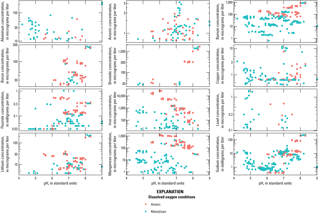
Selected major ion and trace element constituents and pH, grouped by oxic and anoxic water conditions. Anoxic water conditions contain <0.5 milligrams per liter (mg/L) of dissolved oxygen and mixed/oxic water conditions contain ≥0.5 mg/L of dissolved oxygen.
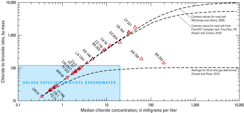
Relation between median chloride concentrations and median chloride: bromide mass ratios in 28 wells in the Pennsylvania Groundwater Monitoring Network. Binary mixing curves are notated to represent various sources of chloride. Blue rectangle represents range of values expected in dilute groundwater.
Nutrients
Nutrients analyzed in this study included nitrogen and phosphorus species. Nitrogen species in water typically include nitrate, nitrite, and ammonia. Phosphorus is mainly present as orthophosphate. Although nutrients are naturally present in soil and rock, excessive concentrations of nutrients usually indicate an anthropogenic source, such as fertilizer or animal wastes, effluent from sewer systems and septic tanks, atmospheric deposition, and stormwater drainage. Excessive nitrate in drinking water can be dangerous for human consumption, especially for infants below the age of 6 months, as it disrupts the transport of oxygen in blood. The majority of well locations in the GWMN are in forested areas, although some wells are located in areas of agricultural land use. Summary statistics of the nutrients analyzed are presented in table 7.
Table 7.
Minimum, median, and maximum concentrations of nutrients for 221 samples collected from 28 wells within the Pennsylvania Groundwater Monitoring Network, 2015–19.[mg/L as N, milligrams per liter as nitrogen; mg/L as P, milligrams per liter as phosphorus; EPA, U.S. Environmental Protection Agency; MCL, maximum contaminant level; SMCL, secondary maximum contaminant level; total, total water sample; total,recov, total water sample, recovered; dissolved, dissolved water sample; --, no MCL or SMCL established]
Dissolved nitrate concentrations ranged from 0.08 to 12.10 mg/L, with a median concentration of 0.50 mg/L. Seven of the 129 (5.4 percent) samples above the reporting limit of 0.04 mg/L that were collected exceeded the EPA MCL of 10 mg/L; all of these samples were collected at the Lebanon County observation well LB 372, which is located in an urban setting and within a carbonate aquifer that is surrounded by heavy agricultural land use. The majority of nitrite samples analyzed had concentrations that were below the reporting limit of 0.01 mg/L. Only four wells (LB 372, AG 700, LA 1201, and VE 57) had concentrations greater than 0.01 mg/L and none were above the EPA MCL of 1.0 mg/L as N. Nitrite concentrations ranged from 0.02 to 0.04 mg/L, with a median concentration of 0.03 mg/L. Dissolved phosphorus concentrations from the 97 samples (44 percent) with concentrations greater than the reporting limit ranged from 0.01 to 0.12 mg/L, and had a median of 0.02 mg/L (table 6). Concentrations for orthophosphate from 89 samples (40 percent) ranged from 0.01 to 0.06 mg/L, with a median concentration of 0.02 mg/L. Orthophosphate concentrations were positively correlated with an increased pH, with samples with pH greater than 7.6 having the highest concentrations in the GWMN (appendix 3)
Dissolved organic carbon (DOC) can alter groundwater quality by acting as a pH buffer, interacting with DO and other ions in oxidation/reduction reactions, and through involvement in mineral dissolution/precipitation reactions (Aiken, 2002). These processes can lead to the increased mobility of metals including lead, copper, and zinc, as well as radionuclides including uranium. DOC was present above the 0.5 mg/L reporting limit in 27 samples (12 percent); concentrations ranged from 0.52 to 2.8 mg/L, with a median concentration of 1 mg/L. None of the samples had DOC greater than 4 mg/L, a concentration indicative of contamination (Regan and others, 2017). Wells with DOC concentrations consistently near the reporting limit include AG 700, BR 203, FO 11, LA 1201, and PO 72. Of the trace elements that are sensitive to elevated DOC, only copper was found regularly in samples with a measurable DOC level. A general positive trend between increasing dissolved copper and DOC concentrations is noted, with the highest values of copper measured in well BR 203. Although the source of copper is uncertain, this well is sampled through copper plumbing, as opposed to Teflon tubing, and copper concentrations are consistent with mobilization caused by the presence of organic compounds in water (Lehman and Mills, 1994).
Volatile Organic Compounds
Volatile organic compounds (VOCs) consist of a range of natural and synthetic carbon-based compounds; their properties include relatively low solubility in water and a high vapor pressure. VOCs are used for a wide range of industrial, commercial, and domestic applications and can enter groundwater through spills or deposition from atmospheric transport. VOCs are commonly found wherever human activities are ongoing; compounds including solvents, fuels, fumigants, and disinfection byproducts can enter the environment through pesticide application, leaking storage tanks, or spills. VOCs have historically been used and disposed of indiscriminately, leading to the widespread presence of these chemicals in the environment. The reporting level of the majority of VOCs sampled was either 0.5 µg/L or 1.0 µg/L; of the 68 VOCs that were sampled during the first sampling event at each well, only one, tribromomethane, was detected.
Tribromomethane was measured at a level of 2 µg/L in well FO 11; this trihalomethane has historically been used as a solvent and is a byproduct of water chlorination processes but is also produced naturally by seaweeds and phytoplankton (Palmer and Reason, 2009). The land use surrounding well FO 11 is almost entirely forested, indicating that tracing the source of the tribromomethane would be difficult.
Radionuclides
Radioactivity is the release of particles and energy from unstable elements as they decay to more stable forms. Radionuclides are naturally present in bedrock and soils and can be dissolved or leached into groundwater. There are three types of radioactive decay: alpha decay, in which positively charged helium particles are released; beta decay, in which positrons or electrons are released from an element; and gamma decay, in which electromagnetic waves are released from an element. Radioactivity in samples collected from the GWMN is measured in picocuries per liter, which is equal to the activity of one nanogram of radium and results are presented in table 8.
Table 8.
Minimum, median, and maximum concentrations of radionuclides for 221 samples collected from 28 wells within the Pennsylvania Groundwater Monitoring Network, 2015–19.[pCi/L, picocuries per liter; µg/L, micrograms per liter; EPA, U.S. Environmental Protection Agency; MCL, maximum contaminant level; SMCL, secondary maximum contaminant level; total, total water sample; dissolved, dissolved water sample; --, no MCL or SMCL established]
| Parameter | Units | Method | Number (percent) above reporting level | Minimum | Median | Maximum | Number (percent) exceeding standard | EPA MCL | EPA SMCL |
|---|---|---|---|---|---|---|---|---|---|
| Gross alpha activity, total | pCi/L | EPA 900.0 | 14 (6) | –4.02 | 0.32 | 6.89 | 0 (0) | 15 | -- |
| Beta radioactivity, total | pCi/L | EPA 900.0 | 23 (10) | –0.26 | 1.83 | 7.57 | 0 (0) | -- | -- |
| Radon-222, total | pCi/L | SM 7500-Ra B | 26 (12) | 40 | 500 | 7050 | 2 (1) | -- | 4,000 |
| Radium-226, total | pCi/L | EPA 903.1 | 22 (10) | 0 | 0.18 | 2.09 | 0 (0) | -- | -- |
| Radium-228, total | pCi/L | Percival and Martin, 1974 | 18 (8) | –0.48 | 0.44 | 1.9 | 0 (0) | -- | -- |
| Uranium, dissolved | µg/L | EPA 200.8 | 36 (16) | 0.33 | 0.67 | 4.83 | 0 (0) | 30 | -- |
| Uranium, total | µg/L | EPA 200.8 | 29 (13) | 0.34 | 0.93 | 4.94 | 0 (0) | 30 | -- |
The isotopes primarily responsible for naturally occurring radioactivity in groundwater are uranium-238 and thorium-232, which are present in minerals. These particles decay over time through a series of steps that emit alpha or beta radiation, producing mostly short-lived daughter products until a stable isotope of lead is produced; the majority of naturally occurring radioactivity is caused by the decay of uranium-238 (Hem, 1985). The half-life of uranium-238 is 4.5 billion years and includes the daughter product radium-226 (half-life of 1,620 years) and radon-222 (half-life of 3.8 days) as it decays to the stable lead-206. Radon-222 is the decay product of radium-226 and is a chemically inert gas that emits alpha particles and is soluble in water.
Radon-222 is considered by the EPA to be the second-leading cause of lung cancer and the leading cause of lung cancer in nonsmokers, with an estimated 20,000 deaths in the United States attributed to it each year (American Cancer Society, 2015). Measured values of radon-222 ranged from 40 to 7,050 pCi/L, with a median concentration of 500 pCi/L. Two wells (CU2 and UN 51) had radon-222 activity levels that were greater than the higher proposed MCL of 4,000 pCi/L, which was created for community water suppliers that use groundwater for some or all of its supply in states that have an enhanced indoor air radon program (U.S. Environmental Protection Agency, 1999; Gross and Cravotta, 2017). In addition, 18 of the 28 wells in the GWMN (fig. 17) contained radon-222 values higher than 300 pCi/L, which is the lower proposed MCL for states that do not have an enhanced indoor air radon program (U.S. Environmental Protection Agency, 2014). Three wells (AG 700, CB 104, and CE 118) do not have radon-222 data available.
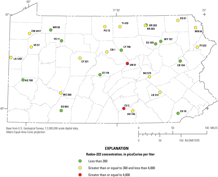
Spatial distribution of radon-222 proposed maximum contaminant level exceedances collected from 28 wells within the Pennsylvania Groundwater Monitoring Network, variously dated.
Gross alpha activity of 14 samples with activities above the reporting level ranged from –4.02 to 6.89 pCi/L, with a median concentration of 0.32 pCi/L, and the gross beta activity of 23 samples ranged from –0.26 to 7.57 pCi/L, with a median concentration of 1.83 pCi/L. Negative activities of gross alpha and beta radiation are the result of the sensitivity of laboratory instruments used to measure radiation; the random nature of radioactive decay makes it possible for background radiation to exceed the activity of the original sample (Brookhaven National Laboratory, 2019). Several wells did not have measurable activities for alpha or beta activity. Six of the wells in the GWMN (AD 146, BR 203, CU 2, LB 372, SQ 61, and WN 64) have reported filtered uranium levels above the reporting limit of 0.328 µg/L; concentrations range from 0.33 to 4.83 µg/L, with a median concentration of 0.67 µg/L. The highest uranium values were recorded at well BR 203. None of the measured concentrations of radium were above the EPA MCL of 30 µg/L.
Dissolved Methane and Other Hydrocarbons
Methane and other hydrocarbons can occur naturally in groundwater owing to anaerobic bacterial processes that break down organic materials in shallow aquifers (biogenic production) or through the breakup of organic matter at elevated temperatures and pressures in deep sedimentary strata (thermogenic production). Biogenic production typically results in hydrocarbons that consist almost entirely of methane, whereas thermogenic production can also contain higher-chain hydrocarbons in addition to methane. Results of hydrocarbon gas analysis are summarized in table 9. Three wells in the GWMN (BR 202, CW 2417, and WR 50) contained dissolved methane levels above the reporting limit of 12 µg/L; concentrations from the three wells ranged from 22 to 8,230 µg/L. None of the methane measurements were above the action level of 10–28 mg/L (10,000 to 28,000 µg/L) recommended by the Department of Interior Office of Surface Mining (Eltschlager and others, 2001), but the recorded concentration of 8.23 mg/L from well WR 50 exceeded the Pennsylvania state action level of 7 mg/L (7,000 µg/L) (Pennsylvania Department of Health, 2019). WR 50 also had the only recorded value for ethane, with 1,890 µg/L; the dissolved sulfate concentrations ranging from 2.7 to 24 mg/L suggest that methanogenesis is not the primary source of hydrocarbons in the well and that there may thermogenic gas present (McMahon and others, 2017). There were no values over the reporting limit for propane or other higher chain hydrocarbons.
Table 9.
Minimum, median, and maximum concentrations of hydrocarbons collected from 28 wells within the Pennsylvania Groundwater Monitoring Network, 2015–19.[µg/L, micrograms per liter; EPA, U.S. Environmental Protection Agency; MCL, maximum contaminant level; SMCL, secondary maximum contaminant level; total, total water sample; dissolved, dissolved water sample; PaDEP, Pennsylvania Department of Environmental Protection; BOL, Bureau of Laboratories; --, no MCL or SMCL established]
Statistical Analysis of Groundwater Quality Data
Statistical analyses of groundwater quality data from the 221 samples collected from 2015 to 2019 were completed to characterize trends and patterns within the GWMN. A range of analyses were used to look for similarities and differences between the wells within the GWMN, changes occurring over time within the wells, and with the sampling design and methods. Results are evaluated in order to inform future decisions regarding changing or expanding the GWMN or sampling protocols.
Principal Components Analysis of Samples
Principal components analysis (PCA) is a statistical method used to identify major factors that can account for variability and associations among variables within a large dataset. The goal of PCA is to reduce the dimensionality by combining those variables on a smaller set of principal components while retaining most of the original variation (Jolliffe, 2010). A PCA transformation of GWMN water-quality data was developed using 200 (90.5 percent) of 221 samples, each of which contained a complete set of constituents used in the model. If a sample had missing values for any particular constituent that entire sample was excluded from the model. Multiple samples from each well are represented in this analysis; one sample season (fall 2016) has incomplete anion data and, consequently, has been excluded from the analysis. To perform the PCA, only dissolved concentrations of constituents were utilized; to incorporate more samples into the model, concentrations that were below the reporting limit were censored to the reporting limit. Constituents that were frequently below detection were excluded, and parameters that are related to physical characteristics of the sample (location, air and water temperature, barometric pressure, and so forth) were also removed from the analysis. Laboratory-measured specific conductance (SC) and alkalinity values were used in the model instead of field measured values to resolve charge balance issues identified with some of the field-measured values. To account for the difference in constituent value ranges, reporting units, and censoring levels, data used in the PCA were standardized by subtracting the mean for the dataset from each value and then dividing the result by the standard deviation.
Collectively, three principal components (PCs) explain 74.5 percent of variability contained in the groundwater quality data of the GWMN and consist of 20 commonly detected constituent loadings; they will be identified as PC1 (dissolved solids), PC2 (redox), and PC3 (sodium-chloride)(table 10). Each PC has strong relations to a subset of specific parameters. These relations are expressed as loadings, which are the positive or negative coefficients between the PC and the parameter (table 10; Thyne and others, 2004). Associations of additional chemical and physical variables excluded from the model are indicated by the Spearman-rank coefficients of correlation of these variables with the PC scores and can be found in the associated data release (Conlon, 2021).
Table 10.
Principal components analysis of major factors controlling the chemistry of wells in the Pennsylvania Groundwater Monitoring Network.[°C, degrees Celsius; PC, principal component; TDS, total dissolved solids; redox, reduction-oxidation; Na, sodium; Cl, chloride]
PC1 (dissolved solids), which explains 50.3 percent of the variability in the data, indicates the effects of mineral weathering on groundwater quality and contains positive loadings for SC; alkalinity; dissolved solids; major ions including calcium, magnesium, sodium, potassium, chloride, sulfate, and fluoride; and pH. PC1 contains negative loadings for dissolved oxygen (table 10, fig. 18A). Individual scores were driven by samples from wells AG 700, BR 202, CN 1, and LB 372 (fig. 18B). In general, greater concentrations of dissolved solids coincide with higher values of specific conductance and pH, which can be attributed to more extensive dissolution of major minerals. Linear regressions show that a positive linear relation with a moderate Pearson correlation (r = 0.67) exists between pH and specific conductance (fig. 19A), while negative relations with weak correlations exist between DO and pH (r = –0.49) (fig. 8) and DO and SC (r = –0.44) (fig. 19B). Generally, pH in GWMN wells was inversely related to DO levels, with the exception of well CE 118, which is located in a carbonate aquifer where high DO reflects the interconnection between subsurface atmosphere and the land surface. Calcium and magnesium, which together contribute to the hardness of water, exhibited strong positive loadings on PC1. Elevated hardness, alkalinity, and pH commonly result from the dissolution of carbonate minerals, including calcite and dolomite, and possibly other minerals including gypsum and pyrite. Positive associations of pH and sodium on PC1, with less significant loadings by chloride, may be attributed to cation exchange, a process whereby sodium and other alkali earth metal ions in clay minerals are mobilized from solids while dissolved calcium and magnesium ions are removed from solution, similar to the operation of a water-softener system (Poth, 1962; Hem, 1985).
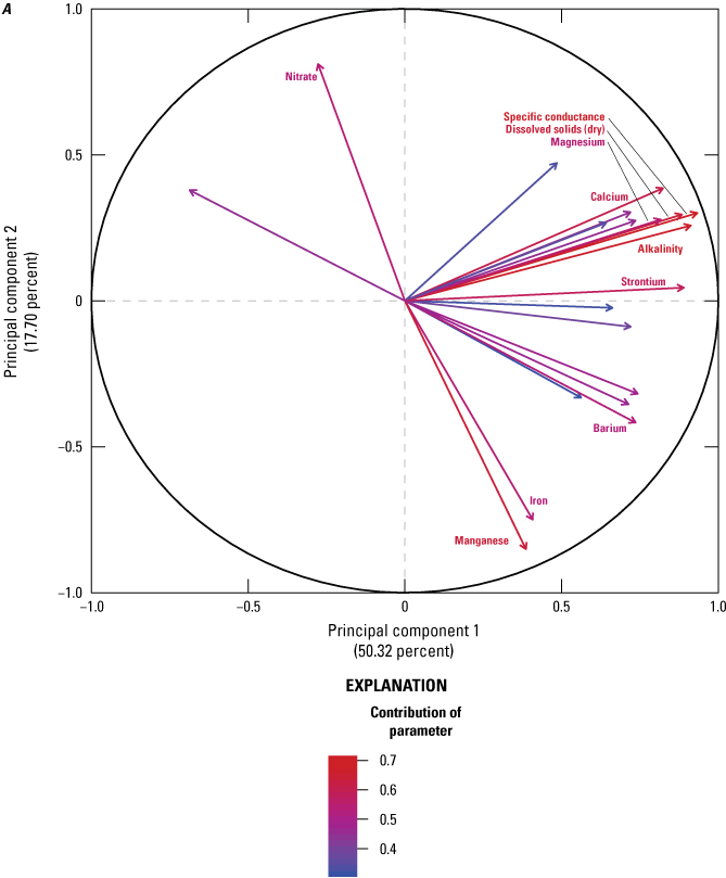
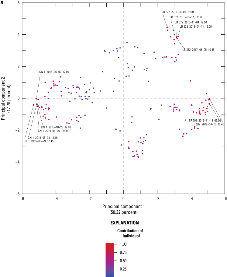
Results of principal components analysis, principal components 1 and 2: parameter variables (A) and individual samples (B) plots.
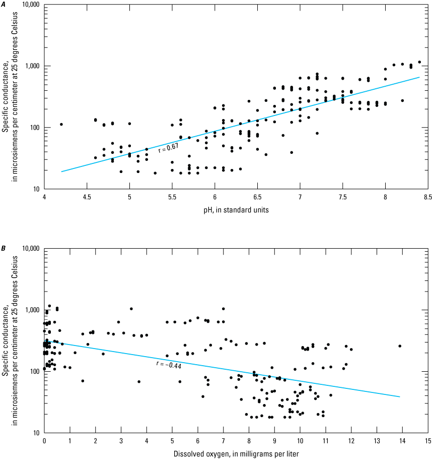
Moderately significant relations between pH and specific conductance (A), and dissolved oxygen and specific conductance (B).
Wells that exhibited oxic conditions (DO >0.5 mg/L) generally contained lower alkalinity and major ion concentrations; the exception are wells located in carbonate aquifers, which contain concentrations above GWMN medians for all dissolved major ions. An inverse relation between DO and major ions suggests that (1) organic materials and soluble minerals, such as those found in carbonate rocks, are not present in the aquifer and (or) (2) recharge is not recent, leading to residence time that is sufficient for extensive interactions between water and bedrock that consume oxygen while releasing ions to solution. End-member wells with the highest individual contributions for PC1 include CN 1, BR 202, and AG 700; CN 1 is a highly oxic water with low ionic strength, whereas BR 202 and AG 700 exhibit some of the highest conductivities and alkalinities in the GWMN (table 1.1, fig. 18B). BR 202, which experiences the highest values for several constituents including sodium, chloride, and bromide, is located in proximity to a sewage treatment facility. The relatively shallow depth of this well (180 ft) combined with its upland topographic location indicates that interaction with deep-water brine is an unlikely cause of the elevated levels of these constituents, and instead suggests interaction between water treated at the plant and the aquifer that the well is drawing from. Scores on PC1 are positively correlated with ammonia and various trace elements including boron and arsenic and negatively correlated with the land surface elevation of a well, suggesting that the higher-elevation wells were the more dominant contributors to this PC (Conlon, 2021).
PC2 (redox) explains an additional 17.7 percent of variability in the dataset and has positive loadings by nitrate, DO, calcium, and chloride with negative loadings by manganese and iron (table 10, fig. 18A). Samples with high contributions to PC2 generally fall into two groups, one which is dominated by carbonate aquifers that have high concentrations of constituents with the positive loadings, and the other that has low concentrations of nitrate and DO with high concentrations of manganese and iron, which is interpreted as older water with prolonged isolation from the atmosphere. Microbial oxidation of organic carbon generally leads to the depletion of DO and nitrate followed by the reduction of solid manganese (III-IV) and iron (III) oxides, with the consequent release of dissolved iron and manganese. The highest individual contributions for PC2 are wells located in carbonate aquifers that have elevated DO and nitrate (LB 372, CE 118, CH 10), with associated high scores, and wells located in sandstone aquifers that have low DO concentrations and elevated iron and manganese (CF 321, FO 11, SO 854), with negative scores (Conlon, 2021). Well CF 321 contains the highest median iron (26,000 µg/L) and manganese (1,220 µg/L) concentrations in the GWMN, but also has low DO and sulfate concentrations with pH ~6, consistent with a reducing environment. The positive sulfate loading coupled with negative loadings by iron and manganese on PC2 indicates that mine drainage is not a contributing factor for this subset of wells. Other wells with positive loadings for PC2 generally exhibited oxic conditions; the negative loadings by iron result from its low solubility in oxidizing environments (Hem, 1985). Scores on PC2 are positively correlated with redox potential (Eh) and uranium, which forms an oxycation (UO2+2) that complexes with carbonate (Conlon, 2021). A positive correlation between PC2 was also seen with the intensity of agricultural land use within a 1,000-m-radius of a well; the subset of wells with high PC2 scores and nitrate concentrations are all located in regions with large-scale agricultural production. Scores on PC2 are negatively correlated with ammonia, which is a reduced form of nitrogen that can be produced by the microbial reduction of nitrate (Hem, 1985; Conlon, 2021). Together, PCs 1 and 2 combine to explain 68.0 percent of the variability within GWMN samples.
PC3 (sodium chloride) accounts for an additional 6.4 percent of the variability in the GWMN; positive loadings include chloride, sodium, and potassium, and negative loadings include phosphorus, fluoride, and pH (table 10). The highest individual contributions to PC3 are from wells CB 104, CU 2, and CF 321 (Conlon, 2021). The samples from these wells, which have negative scores on PC3, are acidic and have molar Na:Cl ratios of approximately 1, consistent with a sodium-chloride source (fig. 20). Wells with low individual scores on PC3, including CE 118 and LA 1201 (Conlon, 2021), generally had higher dissolved solids and pH values along with higher potassium concentrations; these wells occur in limestone aquifer settings where highly conductive flow paths may facilitate the transport of potassium leached from the soil during harvesting seasons (Hem, 1985). Iron and manganese have positive loadings for PC3 whereas that for DO is negative, suggesting that iron and manganese may be elevated in association with low pH (PC3) or reducing conditions (PC2). Scores on PC3 were positively correlated with nickel, which coprecipitates or adsorbs with iron and manganese, and lithium, which is associated with cation exchange processes that also mobilize sodium. PC3 scores were also slightly positively correlated with the intensity of developed land use within a 1,000-m radius of a well, which suggests that de-icing road salts may be a primary source of the positive loadings on this PC (Conlon, 2021). Scores on PC3 were negatively correlated with orthophosphate, which tends to adsorb to aquifer solids at low pH (Hem, 1985).
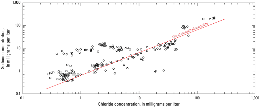
Relation between sodium and chloride concentrations in Pennsylvania Groundwater Monitoring network samples, 2015−19. Line of concentration equality represents a 1:1 equilibrium of sodium and chloride concentrations.
Results of the PCA model were subsequently used to create a hierarchical clustering classification to group wells that are most similar within the GWMN. Using the 200 samples from 28 wells that were used to establish PCs 1 through 3, four sampling clusters were visually identified (table 11); a spatial distribution of the well clusters is shown in figure 21. Cluster 1 contains a positive association with DO and negative associations with most major ions, displaying the contrasting relation that exists in PC1. This subset of wells generally has groundwater that is oxic (DO >0.5 mg/L) and has low ionic strength. Cluster 2 contains positive associations with iron and manganese concentrations and is dominated by wells that exhibit the reducing conditions indicated by negative scores on PC2. Cluster 3 indicates positive associations related to water hardness and nitrate, with contrasting negative correlations by iron and manganese. This cluster contains wells that are located in carbonate aquifers where elevated dissolved solids and nitrate are common characteristics. Cluster 4 contains positive associations with most major ions and a negative association with dissolved oxygen; this cluster contains a range of wells whose behavior is described to varying degrees by PCs 1 and 3.
Table 11.
Results of hierarchical cluster analysis of principal components analysis results of the major factors controlling the chemistry of wells in the Pennsylvania Groundwater Monitoring Network.[+, positive association with a well cluster; -, negative association with a well cluster; SC, specific conductance; TDS, total dissolved solids; DO, dissolved oxygen; Alk, alkalinity; NA, no association]
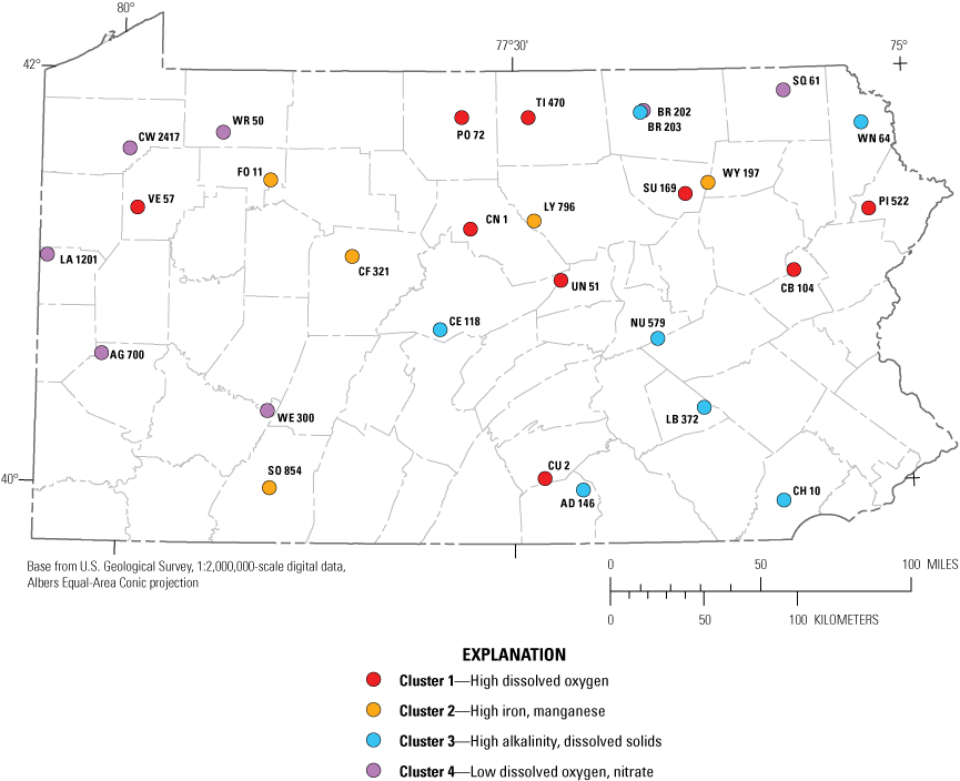
Spatial distribution of clusters from hierarchical clustering of principal components analysis results of 28 wells within the Pennsylvania Groundwater Monitoring Network.
Drought Indicator Relations
The Palmer Drought Severity Index (PDSI) offers a proxy to how wet or dry conditions are in a given location on a monthly time scale; a positive index value indicates that an area has received more precipitation over the previous 1-month time step, whereas a negative index value indicates that less precipitation fell compared to the previous month. Although drought conditions can lead to less runoff infiltrating into aquifers and lower water levels in aquifers, wetter conditions may increase infiltration rates and groundwater flow, leading to greater concentrations of dissolved constituents. A total of 162 samples collected between 2015 and 2018 were used in this analysis; computed PDSI values were not available for 2019. Several dissolved nutrients, major ions, and trace elements were compared to PDSI values from the month the sample was collected in, as well as the PDSI values from each of the 9 months prior to sample collection. Values that are below the reporting limit are replaced with normally distributed random values below the reporting limit for each constituent to account for missing values.
For each constituent and each time lagged PDSI value, a Kendall correlation was computed to determine if PDSI was an accurate indicator of constituent concentrations on a networkwide scale (table 12). Generally, only very weak correlations between time lagged PDSI values and constituent concentrations exist across the GWMN; this is likely a result of the variability of climate, land use, and geologic settings that the wells are located in. The majority of the correlations are negative, indicating that higher constituent concentrations are related to a more negative drought signal (PDSI < 0); the strongest networkwide trend (R = –0.21) existed between orthophosphate and a 7-month lag in PDSI.
Table 12.
Correlation matrix between selected water-quality constituents and time-lagged Palmer Drought Severity Index (PDSI) values collected from 28 wells within the Pennsylvania Groundwater Monitoring Network, 2015–18.Well clusters produced from hierarchical clustering (fig. 22) produced stronger responses to time lagged PDSI values (appendix 4, table 4.1). Cluster 1 (high dissolved oxygen) correlations include a positive association between lithium and nonlagged (R = 0.31) and 1-month lagged (R = 0.32) PDSI, and a negative association between orthophosphate and 8-month lagged (R = –0.31) and 9-month lagged (R = –0.35) PDSI. The positive association between lithium and PDSI suggests that wetter conditions leads to higher concurrent mobility in this subset of wells; correlations between lithium and PDSI gradually become weaker as the time lag increases. Cluster 2 (high iron and manganese) correlations include a strong positive association with lithium and a moderately positive association with chloride and concurrent PDSI, as well as moderately negative correlations with phosphate, orthophosphate, magnesium, and potassium. The influence of current drought conditions is noted for this subset of wells, as correlations become weaker as the lag of PDSI values increases. Cluster 3 (high alkalinity and dissolved solids) generally exhibited very weak correlations with PDSI; a weak negative association was found between lithium and concurrent PDSI (R = –0.33). This subset of wells exists in areas with carbonate geology, which suggests that overall, they are less responsive to changes in the drought index than all of the wells in the GWMN. Cluster 4 (low dissolved oxygen and nitrate) correlations showed only very weak correlations between constituents and PDSI, which suggests that this group of wells, all of which are located in the Appalachian Plateaus physiographic province, are not responsive to changes in precipitation patterns. In general, selected constituents in subsets of wells determined by hierarchical clustering offer a stronger response to changes in PDSI than seen on a networkwide scale, which indicates that other factors, including local geology and land use, are important in the response to changes in precipitation.
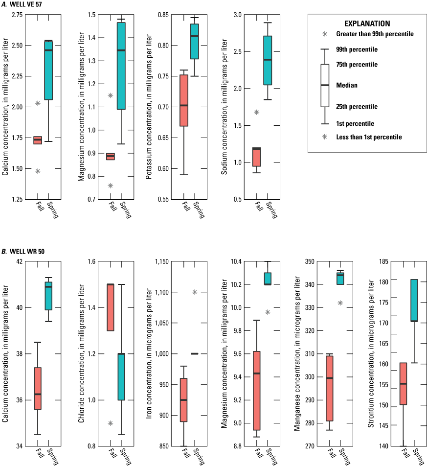
Seasonal differences in selected constituent concentrations in wells VE 57 (A) and WR 50 (B).
Seasonality
Biannual sampling results were examined to look for changes in constituent concentrations that may be attributed to the sampling season that the sample was collected in. Wells within the GWMN generally followed a pattern of higher winter and spring water levels and lower summer and fall water levels (fig. 4), which indicates that seasonality in the hydrologic data is present. As discussed in the preceding section, the time of year when samples are collected is important when considering antecedent precipitation. Infiltration of precipitation in the form of rain or snowfall is affected by changes in evapotranspiration owing to air temperature and plant activity, which result in changes to the amount of water entering aquifers (Pennsylvania Geological Survey and Pittsburgh Geological Society, 1999). Seasonal surface loading of some constituents may also be affected by seasonal human activities; for instance, nitrogen and phosphorus loading may occur in areas that are dominated by agricultural activity as fields are fertilized, whereas increased levels of ions such as sodium, chloride, and magnesium may occur in areas with road treatments that use de-icing salts.
Wilcoxon rank-sum tests were used to compare several constituents that have been sampled throughout the GWMN over the course of several spring and fall sampling seasons. Tests were completed for all wells in the GWMN and on a subset of wells that had sufficient data to examine the seasonal differences on an individual scale. Of the 221 sampling events that have occurred since the inception of the GWMN, 100 samples have been collected in the spring (generally in April and May) and 121 samples have been collected in the fall (generally in October and November). Exact Wilcoxon rank-sum tests were applied for constituents that had values above the reporting limit for more than 50 percent of samples during both the spring and fall sampling periods, with data from all available samples from wells in the GWMN. With a significance level of P = 0.05, there are no filtered or unfiltered parameters that show a significant difference between the spring and fall sampling seasons, suggesting that there are no statewide patterns of constituent increases or decreases based on sampling season.
The second set of exact Wilcoxon rank-sum tests on seasonality examined samples from 16 of the 28 wells in the GWMN that have been sampled at least 8 times, with at least 4 spring and fall samples each. For these wells, 45 parameters with a sufficient number of results were used to perform Wilcoxon rank-sum tests between fall and spring sampling for at least one well. Results based on the number of significant differences (P <0.05) using a two-sided alternative hypothesis are presented for individual parameters (table 13) and for wells (table 14); the counts represent the number of instances where a parameter or a well exhibit a difference between spring and fall samples. A graphical representation of this data is available in appendix 5. Of the 16 wells, VE 57 and WR 50 contained the most differences between spring and fall samples, with each well exhibiting significant differences for 16 constituents; for both wells, concentrations were higher during the spring sampling season. The differences seen in VE 57 (fig. 22A) were largely in major ion concentrations, whereas the differences in WR 50 (fig. 22B) also include iron, manganese, and strontium. Other wells that contained numerous differences between spring and fall samples include UN 51 (8 differences), WN 64 (8 differences), and TI 470 (3 differences)(table 14). Twenty-nine of the 45 parameters had a significant difference between spring and fall sampling for at least one of the 16 wells. Filtered and total sodium levels were significantly different for four wells (table 13; CB 104, UN 51, VE 57, WN 64). Analysis of one-tailed results of Wilcoxon rank-sum tests indicates that differences between spring and fall samples for individual wells generally follow a pattern of concentrations being higher in the spring than the fall; graphical results of comparisons between spring and fall sampling seasons for each well can be found in appendix 5. Of the 16 wells examined in these tests, only two (AG 700 and CU 2) did not display any significantly different constituent concentrations between the spring and fall sampling seasons (table 14); this indicates that although the magnitude of changes varies from well to well, seasonal fluctuations in constituent concentrations are common in a wide range of settings across the State.
Table 13.
Counts of Wilcoxon rank-sum tests with significant results comparing spring and fall sampling seasons for selected constituents from 16 wells with long term records within the Pennsylvania Groundwater Monitoring Network, 2015–19.[wu, unfiltered water sample; wu,recov, unfiltered water sample, recovered; wf, filtered water sample; °C, degrees Celsius; fixedEP,lab:fixed endpoint, laboratory; NephRatio, nephelometric turbidity ratio units; --, not applicable or none]
Multi-Year Constituent Trends
Increases or decreases in constituents over an extended period of time may indicate that aquifers are experiencing long-term changes to ambient groundwater quality. Changes may be the result of a variety of factors including but not limited to, precipitation patterns, road salt application, nutrient runoff from agricultural areas, and growth of developed areas that are proximal to sampling sites. The Mann-Kendall trend test was used to determine whether there are positive or negative trends among constituents in wells that have been sampled for at least four spring and four fall sampling seasons (Yue and others, 2002). The Mann-Kendall trend test is a nonparametric analysis for monotonically increasing or decreasing trends. Median values from 15 wells were calculated for each of the 10 sampling seasons between spring 2015 and fall 2019; one well, AG 700, was left out of this long-term analysis owing to missing sample data from the spring and fall 2015 sampling seasons. The trend tests used a censored dataset that contains reporting limits substituted for missing data in cases where the concentrations of a particular constituent were below the reporting limit. A list of parameters included in the analysis, along with P-values and the direction of change that was observed over time are shown in table 15; a positive number indicates an increasing trend, whereas a negative number indicates a decreasing trend.
Table 15.
Mann-Kendall trend test results on a network scale for 15 wells within the Pennsylvania Groundwater Monitoring Network, 2015–19.[wu, unfiltered water sample; wu,recov, unfiltered water sample, recovered; wf, filtered water sample; Statistic, Z quantile of the standard normal distribution. Positive values indicate an increasing trend over time and negative values indicate a decreasing trend over time]
Generally, large increasing or decreasing trends were not observed on a statewide scale, in part owing to the diversity of settings of the GWMN wells and the relatively short period of current monitoring (2015–19). The only parameter that exhibited a significant change (P <0.05) over the period of record was total magnesium (P = 0.032). Both total and filtered magnesium (P = 0.074) showed an increasing trend over time, as did several other constituents including sodium and potassium. Decreasing trends over time were observed for constituents including calcium, iron, and manganese, although none of these trends are considered significant. Although changes were not apparent on a statewide scale, trends (significant or not) are more pronounced at individual sampling sites where factors affecting constituent levels have a direct impact on the water chemistry of a particular well. Forty-two parameters exhibited a significant change (P <0.05) over the period of record in at least 1 well (table 16); constituents including thallium (filtered and unfiltered), cadmium (filtered), beryllium (unfiltered), and sodium (filtered) showed a positive or negative change in at least one-third of the 15 wells with long-term data. Of the 87 significant changes, 69 indicated increasing trends and 18 indicated decreasing trends over time. Field parameters including water temperature, specific conductance, pH, and dissolved oxygen were generally consistent over time in most wells, with only nine significant trend changes over time. Filtered chemical constituents exhibited 38 significant trend changes over time whereas unfiltered chemical constituents exhibited 40 significand trend changes over time, although many of these differences were on the order of <1 mg/L for major ions or <1 µg/L for trace elements. Many parameters including silver, selenium, mercury, nitrite, and ammonia lacked enough results to perform trend analysis in more than half of the wells with long term records. Each of the 15 wells with long-term data contained at least one parameter with a significant change; SQ 61 (12 parameters), UN 51 (12 parameters), and CB 104 (11 parameters) exhibited the most changes over time, whereas CN 1 (1 parameter), VE 57 (3 parameters), and FO 11 (3 parameters) showed the least amount of change; the number of significant trends seen in a particular well appears to be unrelated to the well clusters described in the PCA results.
Table 16.
Mann-Kendall trend test results for individual wells within the Pennsylvania Groundwater Monitoring Network, 2015–19.[N, nitrogen; °C, degrees Celsius; --, no data or not applicable]
Considerations for Future Work
Ongoing and future sampling and expansion of wells in the present GWMN will help gain a more comprehensive understanding of ambient groundwater quality in the State of Pennsylvania. Additionally, new wells may be considered for addition to the GWMN, while sampling at others may be curtailed or suspended. This, along with further suggestions for maintaining data quality and data management practices, are explained below.
Modifications to Sampling
Considerations for changes and adaptations of the sampling interval and protocol for the GWMN are largely focused on more frequent data collection of constituents that are only sampled once or periodically. Currently, radiochemicals, hydrocarbons, and VOCs are only collected during the first sampling event at a well. Although many of the samples collected for these constituents are below the established reporting limits, a modified sampling frequency (in other words, once every 5 to 10 years), particularly at wells with previous measurable VOC concentrations, may be useful for determining if more frequent monitoring is necessary for specific wells or constituents. Conversely, as the GWMN is sampled only twice per calendar year, short-term changes that may occur in the GWMN are not currently well-understood. Sampling of a subset of the GWMN at an increased frequency over a period of time may help to determine if events like heavy precipitation affect water quality at a time scale that semiannual sampling does not capture; this information could be used to identify the best times to sample particular wells to get the most representative samples of ambient groundwater quality while also enumerating the time scale at which the water chemistry of wells changes and then recovers to ambient conditions (Mathany and others, 2019).
Expanding the range of parameters that are collected may also benefit the interpretation of GWMN sampling results. Extended sampling of hydrocarbons (including isotopic signature ratios), particularly at wells with detectable levels of methane, may be useful for determining whether the origin of methane is biogenic or thermogenic. In turn, this information could be useful as a proxy for the age of groundwater, as thermogenic gases are commonly produced at depth, whereas the biological production of methane from anaerobic decomposition of organic materials typically occurs at shallower depths (McMahon and others, 2019). A synoptic sampling of age tracers, including but not limited to tritium and sulfur hexafluoride, may be beneficial for gaining a greater understanding of groundwater age, mixing, and the implications it has for the transport time of various constituents in groundwater. Age-dating techniques can be employed to determine the recharge rates of aquifers, while also inferring the susceptibility of those aquifers to surface contamination sources; the presence of modern waters indicates the possibility of rapid recharge and a higher potential for the introduction of contamination (Lindsey and others, 2019). In addition, results from age tracer sampling could inform on the frequency necessary to sample each well in the GWMN; wells with premodern water may need less frequent sample collection to adequately characterize groundwater chemistry. Currently, age-dating analysis has only been performed on a few of the wells in the GWMN; these results are not presented in this report, but the range of groundwater ages from wells of similar design and physiographic setting suggest that aquifer connection to atmospheric deposition varies greatly across the GWMN. Examination of PCA indicates an inverse relation between DO levels and several major ions, which may be indicative of recent recharge in some of the wells within the GWMN that contain high DO levels.
Analysis of differences between total and dissolved concentrations of constituents including major ions, trace elements, and nutrients showed that some parameters are more likely than others to have differences between samples collected with and without filtration. Major ions, which are largely present in solution in the GWMN, do not show statistical differences between total and dissolved samples. Several trace elements, as well as phosphorus, show statistical differences between total and dissolved concentrations because of the lower solubility of these elements, making the collection of both values more important when evaluating water quality of wells within the GWMN. Taken together, these results can inform on updating or modifying sampling schedules to reduce to the duplicative collection of samples.
Plans for monitoring the GWMN over a long period of time allow for analysis of trends on both a network and an individual well scale; maintaining the active sampling status of the wells in the GWMN allows for greater power of statistical analysis. Currently, 16 of the wells have 8 or more samples that were collected on a semiannual schedule, a number that was used as a threshold for inclusion in long-term trend analyses; continued monitoring of this subset of GWMN will provide additional information for characterizing long-term patterns and changes in ambient groundwater quality.
Modifications to Network Design
Results of the current study indicate that future interpretations of data from the GWMN would likely benefit from (1) ensuring that the sample collection procedures and equipment at each well are of similar design, and (2) choosing wells that produce water indicative of ambient conditions in a given part of the State of Pennsylvania. Some of the wells currently sampled in the GWMN have water chemistry that differs greatly from the general concentration distributions of constituents across the GWMN; these wells may be affected by local factors that do not represent ambient groundwater quality on a larger scale within the State. Wells BR 202 and BR 203 are not sampled through dedicated pumps and inert tubing as the rest of the GWMN is; rather, the water collected for these samples arrives at the sampling point after travelling through plumbing that contains copper and other metals. Copper concentrations in well BR 203 considerably exceed values measured at every other well in the GWMN; the presence of DOC may facilitate the dissolution of copper from the plumbing fixtures in the well. BR 202 may not be representative of ambient groundwater quality, as it contains elevated levels of several elements including sodium, chloride, barium, and fluoride. This well is located in proximity to a water treatment facility, which may impact local groundwater quality; additionally, a local source of brine may be present. Further investigation would be needed to appropriately determine the source of water in this well.
In general, some wells as currently configured may not meet ambient groundwater-quality monitoring criteria for a variety of reasons including plumbing design deficiencies and anomalous water-quality constituent data that are not reflective of ambient water quality. Removing these wells from future GWMN sampling events may be appropriate despite these wells having been included in several rounds of sampling owing to the aforementioned deficiencies. Although previously collected data are valuable for understanding local conditions, the design differences at these wells may make comparisons to other wells in the GWMN more difficult owing to the known deficiencies that exist; furthermore, changes to sampling equipment would necessitate differentiating between samples that were collected before or after equipment changes were made.
The analyses presented in this report indicate that interpretations of the data from the GWMN would benefit if future additions to the GWMN included an attempt to use consistent well-sampling designs to remove the variability that is associated with changes in the sampling mechanisms in wells. This could include using similar pumps, tubing, and pipe fittings to ensure that any background levels of constituents that are the result of the equipment used are constant across the GWMN as well as performing QA/QC procedures that ensure the quality of this equipment. Ideally, prospective new wells would be pumped to ascertain field parameters and the specific capacity of the well before it is added to the GWMN.
Underrepresented aquifers in the State could be prioritized when seeking to add wells. These areas include the various surficial, siliciclastic, and carbonate aquifers in the Great Lakes, Pittsburgh Low Plateaus, Appalachian Mountains, and Great Valley physiographic sections of the State. Including new wells in these regions would allow for more detailed statistical analysis to compare water types between various aquifers and physiographic provinces, thus furthering the goal of characterizing ambient groundwaters in spatially diverse parts of the State. Future additions to the GWMN could also be considered for continuous (1-hour data collection interval) monitoring of water levels; currently, a subset of wells in the GWMN do not have continuous water-level monitoring, making it difficult to analyze the effect that rising or falling water levels might have on constituent concentrations. Water-level data would supplement the examination of both long-term trends of constituent concentrations as well as provide more insight on the recharge patterns and cycles of the wells in the GWMN.
Summary
The Pennsylvania Groundwater Monitoring Network (GWMN) was initiated in 2014 with 17 wells located in largely rural areas across the State of Pennsylvania through coordination with the Pennsylvania Department of Environmental Protection (PaDEP), with a goal of characterizing the ambient groundwater quality at several fixed stations around the State. Additional sampling points added to GWMN following its inception have brought the total number of wells sampled semiannually to 28, spread across 27 counties. Wells are typically sampled once in the spring and once in the fall each year for a range of constituents including filtered and unfiltered major and trace elements, nutrients, and organic compounds. Additional sampling that occurs during the initial sampling event at each well includes volatile organic compounds, radionuclides, and hydrocarbons.
Summary statistics for 221 groundwater quality samples from the GWMN collected between 2014 and 2019 are presented and are grouped by constituent type. Nitrate concentrations consistently exceeded the U.S. Environmental Protection Agency (EPA) maximum contaminant level (MCL) in well LB 372. Iron, manganese, and aluminum exceeded the secondary maximum contaminant level (SMCL) in wells including AG 700, CF 321, CW 2417, FO 11, LA 1201, LY 796, SO 854, WR 50, and WY 197. SMCL exceedances were also recorded for pH field readings, with many wells having a pH consistently lower than the recommended 6.5–8.5 range. Two wells (CU 2 and UN 51) contained radon levels greater than the higher EPA action level of 4,000 picocuries per liter (pCi/L), and 18 of the wells contained radon levels higher than the lower 300 pCi/L EPA action level.
Principal components analysis (PCA) was performed on 200 of 221 groundwater-quality samples to determine the driving factors of water quality within the GWMN. Results of the PCA were correlated to additional parameters not included in the PCA to understand relations between principal components (PCs), various parameters, and categorical variables that are not expressed in the model. Three PCs (dissolved solids, redox, and sodium-chloride) collectively explained 74.5 percent of variance seen in GWMN samples. Hierarchical clustering of samples based on PCs 1 and 2 indicate four distinct clusters of wells that have similar chemical and geological characteristics.
Nonparametric Wilcoxon rank-sum tests were employed to test for differences between paired filtered and unfiltered constituents, and differences between samples taken in the spring and in the fall. Rank-sum tests were used for these comparisons to account for the non-normal spread that is common in environmental data. Results showed that there are minimal differences between filtered and unfiltered constituent values except in cases where a low-solubility constituent is more likely to be present in suspension, such as iron and manganese. Correlations between time-lagged Palmer Drought Severity Index values and constituent concentrations were not seen on a networkwide scale, but relations were identified between wells in cluster 2 for chloride, lithium, potassium, fluoride, phosphorus, and orthophosphate.
Comparisons between spring and fall sampling were completed on both a statewide and an individual well scale. Results from the statewide analysis indicate that there are no constituents that show appreciable differences between spring and fall sampling. For individual well seasonal analysis, only the 16 wells with a long-term record (at least 4 spring and 4 fall samples) were included; wells WR 50 and VE 57 showed the most significant differences between spring and fall sampling, with higher concentrations of calcium and magnesium being measured during the spring sampling seasons. Analysis of filtered and unfiltered sodium showed significant differences in 4 (25 percent) of the 16 wells, and many other major ion constituents, including calcium, magnesium, chloride, and fluoride showed a seasonal difference in at least one well.
Long-term constituent trends were evaluated using the nonparametric Mann-Kendall trend test. Median values for selected field parameters and major ion, trace element, and nutrient constituents for 15 wells with a long-term record (at least 8 samples beginning with the spring 2015 sampling season) were computed for each sampling season as well as for the individual wells. Results of the trend tests indicate that although there are statistically significant concentration increases and decreases over time for a range of constituents, the majority of these trend changes are small in magnitude and do not indicate major changes to water quality in the wells. Trend tests were limited by the small sample size; however, future sampling will be helpful for such analysis of an expanded dataset.
Considerations for adaptive monitoring are presented to discuss ways that the sampling and GWMN design can be modified to strengthen the quality of data collected in future GWMN groundwater quality samples. Future additions to the GWMN would benefit from focusing on sampling in physiographic regions of the State that are not currently sampled, with efforts being made to ensure that well and sampling design are comparable to current GWMN specifications. The sampling of additional parameters, specifically emerging contaminants that have not been extensively studied in the ambient aquifers of the State, as well as the resampling of parameters that were sampled during the initiation of the GWMN has the potential to provide greater detail about how these aquifers are changing over time with respect to human and natural influences.
References Cited
Aiken, G., 2002, Organic matter in ground water: U.S. Geological Survey Open-File Report 02–89, p. 21–23, accessed May 13, 2020, at https://water.usgs.gov/ogw/pubs/ofr0289/ga_organic.htm.
Alley, W.M., 1984, The Palmer Drought Severity Index—Limitations and assumptions: Journal of Climate and Applied Meteorology, v. 23, no. 7, p. 1100–1109, accessed May 21, 2020, at https://journals.ametsoc.org/doi/pdf/10.1175/1520-0450%281984%29023%3C1100%3ATPDSIL%3E2.0.CO%3B2.
American Cancer Society, 2015, Radon and cancer: American Cancer Society web page, accessed April 2, 2020, at https://www.cancer.org/cancer/cancer-causes/radiation-exposure/radon.html.
Beck, H.E., Zimmermann, N.E., McVicar, T.R., Vergopolan, N., Berg, A., and Wood, E.F., 2018, Present and future Koppen-Geiger climate classification maps at 1-km resolution: Scientific Data, v. 5, article 180214, accessed September 21, 2020, at https://www.ncbi.nlm.nih.gov/pmc/articles/PMC6207062/.
Belitz, K., Jurgens, B.C., and Johnson, T.D., 2016, Potential corrosivity of untreated groundwater in the United States: U.S. Geological Survey Scientific Investigations Report 2016–5092, 16 p., accessed April 2020 at https//doi.org/10.3133/sir20165092.
Belitz, K., Watson, E., Johnson, T.D., and Sharpe, J., 2018, Secondary hydrogeological regions of the conterminous United States: Ground Water, v. 57, no. 3, p. 367–377, accessed January 19, 2021, at https://ngwa.onlinelibrary.wiley.com/doi/epdf/10.1111/gwat.12806.
Brookhaven National Laboratory, 2019, Site environmental report, volume 1, 2018: Environment Reporter, v. 1, 214 p., accessed July 28, 2020, at https://www.bnl.gov/esh/env/ser/2018SER/2018SER-FullBooklet-Final-2019.pdf.
Chapman, M.J., Cravotta, C.A., III, Szabo, Z., and Lindsey, B.D., 2013, Naturally occurring contaminants in the Piedmont and Blue Ridge crystalline-rock aquifers and Piedmont Early Mesozoic basin siliciclastic-rock aquifers, eastern United States, 1994–2008: U.S. Geological Survey Scientific Investigations Report 2013–5072, 90 p., accessed June 2020 at https://pubs.usgs.gov/sir/2013/5072/pdf/sir2013-5072.pdf.
Clune, J.W., and Cravotta, C.A., III, 2019, Drinking water health standards comparison and chemical analysis of groundwater for 72 domestic wells in Bradford County, Pennsylvania, 2016 (ver. 1.2, May 30, 2019): U.S. Geological Survey Scientific Investigations Report 2018–5170, 66 p., accessed March 2020 at https//doi.org/10.3133/sir20185170.
Clune, J.W., and Cravotta, C.A., III, 2020, Groundwater quality in relation to drinking water health standards and hydrogeologic and geochemical characteristics for 54 domestic wells in Clinton County, Pennsylvania, 2017: U.S. Geological Survey Scientific Investigations Report 2020–5022, 72 p., accessed March 2020 at https//doi.org/10.3133/sir20205022.
Conlon, M.D., 2021, Data for characterization of ambient groundwater quality within a state-wide, fixed station monitoring network in Pennsylvania, 2015–2019: U.S. Geological Survey data release, https://doi.org/10.5066/P9NWQW7C.
Dai, A., and National Center for Atmospheric Research staff, eds., 2019, The climate data guide—Palmer Drought Severity Index (PDSI) (December 12, 2019): National Center for Atmospheric Research web page, accessed March 2020 at https://climatedataguide.ucar.edu/climate-data/palmer-drought-severity-index-pdsi.
Davis, S.N., Whittemore, D.O., and Fabryka-Martin, J., 1998, Uses of chloride/bromide ratios in studies of potable water: Ground Water, v. 36, no. 2, p. 338–350, accessed December 15, 2020, at https://doi.org/10.1111/j.1745-6584.1998.tb01099.x.
DeCicco, L.A., and Hirsch, R.M., 2021, Introduction to the dataRetrieval package: The Comprehensive R Archive Network, accessed January 2020 at https://cran.r-project.org/web/packages/dataRetrieval/vignettes/dataRetrieval.html.
DeSimone, L.A., 2009, Quality of water from domestic wells in principal aquifers of the United States, 1991–2004: U.S. Geological Survey Scientific Investigations Report 2008–5227, 139 p., accessed October 2017 at http://pubs.usgs. gov/sir/2008/5227.
Dieter, C.A., Linsey, K.S., Caldwell, R.R., Harris, M.A., Ivahnenko, T.I., Lovelace, J.K., Maupin, M.A., and Barber, N.L., 2018a, Estimated use of water in the United States county-level data for 2015 (ver. 2.0, June 2018): U.S. Geological Survey data release, accessed March 2020 at https://doi.org/10.5066/F7TB15V5.
Dieter, C.A., Maupin, M.A., Caldwell, R.R., Harris, M.A., Ivahnenko, T.I., Lovelace, J.K., Barber, N.L., and Linsey, K.S., 2018b, Estimated use of water in the United States in 2015: U.S. Geological Survey Circular 1441, 65 p., accessed June 2020 at https://doi.org/10.3133/cir1441. [Supersedes USGS Open-File Report 2017–1131.]
Dresel, P.E., and Rose, A.W., 2010, Chemistry and origin of oil and gas brines in western Pennsylvania (ser. 4): Pennsylvania Geological Survey, Open-File Report OFOG 10–01.0, 48 p., accessed December 15, 2020, at http://citeseerx.ist.psu.edu/viewdoc/download?doi=10.1.1.433.1030&rep=rep1&type=pdf.
Dufor, C.N., and Becker, E., 1964, Public water supplies of the 100 largest cities in the United States, 1962: U.S. Geological Survey Water-Supply Paper 1812, 364 p, accessed June 16, 2016, at https://pubs.er.usgs.gov/publication/wsp1812.
Eltschlager, K.K., Hawkins, J.W., Ehler, W.C., and Baldassare, F., 2001, Technical measures for the investigation and mitigation of fugitive methane hazards in areas of coal mining: Pittsburgh, Pa., U.S. Department of the Interior, Office of Surface Mining Reclamation and Enforcement, Appalachian Region Coordination Center, 129 p., accessed March 28, 2020, at https://semspub.epa.gov/work/05/936303.pdf.
Fishman, M.J., and Friedman, L.C., 1987, Methods for determination of inorganic substances in water and fluvial sediments: U.S. Geological Survey Techniques of Water-Resources Investigations, book 5, chap. A1, 545 p., accessed May 2020 at https://pubs.usgs.gov/twri/05a01/report.pdf.
Gross, E.L., and Cravotta, C.A., III, 2017, Groundwater quality for 75 domestic wells in Lycoming County, Pennsylvania, 2014: U.S. Geological Survey Scientific Investigations Report 2016–5143, 74 p., accessed March 2020 at https://doi.org 10.3133/sir20165143.
Helsel, D.R., Hirsch, R.M., Ryberg, K.R., Archfield, S.A., and Gilroy, E.J., 2020, Statistical methods in water resources: U.S. Geological Survey Techniques and Methods, book 4, chap. A3, 458 p., accessed February 2020 at https://doi.org/10.3133/tm4a3. [Supersedes U.S. Geological Survey Techniques of Water-Resources Investigations, book 4, chap. A3, ver. 1.1.]
Hem, J.D., 1985, Study and interpretation of the chemical characteristics of natural water (3d ed.): U.S. Geological Survey Water-Supply Paper 2254, 264 p., accessed March 12, 2020, at https://pubs.usgs.gov/wsp/wsp2254/.
Höhn, R., Isenbeck-Schröter, M., Kent, D.B., Davis, J.A., Jakobsen, R., Jann, S., Niedan, V., Scholz, C., Stadler, S., and Tretner, A., 2006, Tracer test with As(V) under variable redox conditions controlling arsenic transport in the presence of elevated ferrous iron concentrations: Journal of Contaminant Hydrology, v. 88, p. 36–54, accessed July 2020 at https://doi.org/10.1016/j.jconhyd.2006.06.001.
Hothorn, T., and Hornik, K., 2019, exactRankTests—Exact distributions for rank and permutation tests—R package (ver. 0.8–31): R Foundation for Statistical Computing software release, accessed July 2020 at https://cran.r-project.org/web/packages/exactRankTests/index.html.
Jenness, J., 2006, Topographic position index (TPI) v. 1.2: Flagstaff, Ariz., Jenness Enterprises web page, accessed May 15, 2020, at http://www.jennessent.com/downloads/TPI_Documentation_online.pdf.
Johnson, M., 2020, ClimateR—A set of functions to subset climate data to an area of interest: GitHub web page software release, accessed April 2020 at https://github.com/mikejohnson51/climateR.
Kaiser, H.F., 1960, The application of electronic computers to factor analysis: Educational and Psychological Measurement, v. 20, no. 1, p. 141–151, accessed June 2020 at https://doi.org/10.1177/001316446002000116.
Lê, S.J.J., and Husson, F., 2008, FactoMineR—A package for multivariate analysis: Journal of Statistical Software, v. 25, no. 1, p. 1–18, accessed May 2020 at https://doi.org/10.18637/jss.v025.i01.
Lehman, R.M., and Mills, A.L., 1994, Field evidence for copper mobilization by dissolved organic matter: Water Research, v. 28, no. 12, p. 2487–2497, accessed April 2020 at https://doi.org/10.1016/0043-1354(94)90067-1.
Lindsey, B.D., Jurgens, B.C., and Belitz, K., 2019, Tritium as an indicator of modern, mixed, and premodern groundwater age: U.S. Geological Survey Scientific Investigations Report 2019–5090, 18 p., accessed June 2020 at https://doi.org/10.3133/sir20195090.
Lorenz, D.L., and Diekoff, A.L., 2017, smwrGraphs—An R package for graphic hydrologic data (ver. 1.1.2): U.S. Geological Survey Open-File Report 2016–1188, 17 p., accessed May 2020 at https://doi.org/10.3133/ofr20161188. [Supersedes U.S. Geological Survey Open-File Report 2015–1202.]
Lovely, D.R., and Chapelle, F.H., 1995, Deep subsurface microbial processes: Reviews of Geophysics, v. 33, no. 3, p. 365–381, accessed August 2020 at https://agupubs.onlinelibrary.wiley.com/doi/abs/10.1029/95RG01305.
Mathany, T.M., Saraceno, J.F., and Kulongoski, J.T., 2019, Guidelines and standard procedures for high-frequency groundwater-quality monitoring stations—Design, operation, and record computation: U.S. Geological Survey Techniques and Methods, book 1, chap. D7, 54 p., accessed March 2020 at https://doi.org/10.3133/tm1D7.
McMahon, P.B., Belitz, K., Barlow, J.R.B., and Jurgens, B.C., 2017, Methane in aquifers used for public supply in the United States: Applied Geochemistry, v. 84, p. 337–347, accessed March 2020 at https://doi.org/10.1016/j.apgeochem.2017.07.014.
McMahon, P.B., and Chapelle, F.H., 2008, Redox processes and water quality of selected principal aquifer systems: Ground Water, v. 46, no. 2, p. 259–271, accessed March 27, 2020, at https://ngwa.onlinelibrary.wiley.com/doi/full/10.1111/j.1745-6584.2007.00385.x.
McMahon, P.B., Lindsey, B.D., Conlon, M.D., Hunt, A.G., Belitz, K., Jurgens, B.C., and Varela, B.A., 2019, Hydrocarbons in upland groundwater, Marcellus Shale region, northeastern Pennsylvania and southern New York, U.S.A: Environmental Science & Technology, v. 53, no. 14, p. 8027–8035, accessed April 2020 at https://doi.org/10.1021/acs.est.9b01440.
National Water Quality Monitoring Council, 2020, Water quality data: National Water Quality Monitoring Council online database, accessed March 23, 2020, at https://www.waterqualitydata.us/portal/.
National Weather Service, 2020, Normal snowfall in central PA: National Oceanic and Atmospheric Administration, National Weather Service web page, accessed January 5, 2021, at https://www.weather.gov/ctp/snowNormals.
Norman, J.E., Toccalino, P.L., and Morman, S.A., 2018, Health-based screening levels for evaluating water-quality data (2d ed.): U.S. Geological Survey web page, accessed April 2020 at https://doi.org/10.5066/F71C1TWP.
Palmer, C.J., and Reason, C.J., 2009, Relationships of surface bromoform concentrations with mixed layer depth and salinity in the tropical oceans: Global Biogeochemical Cycles, v. 23, no. 2, GB2014, accessed June 2020 at https//doi.org/10.1029/2008GB003338.
Parkhurst, D.L., and Appelo, C.A.J., 2013, Description of input and examples for PHREEQC version 3—A computer program for speciation, batch-reaction, one-dimensional transport, and inverse geochemical calculations: U.S. Geological Survey Techniques and Methods, book 6, chap. A43, 497 p., accessed October 2020 at https://pubs.usgs.gov/tm/06/a43/.
PennState Extension, 2016, Private water system FAQs: University Park, Pa., Pennsylvania State University, College of Agricultural Sciences web page, accessed May 1, 2020, at https://extension.psu.edu/private-water-systems-faqs.
Pennsylvania Bureau of Topographic and Geologic Survey, 1998, Preliminary landform subdivisions of Pennsylvania, 1998: Pennsylvania Bureau of Topographic and Geologic Survey, Department of Conservation and Natural Resources online database, accessed June 23, 2008, at http://www.pasda.psu.edu.
Pennsylvania Bureau of Topographic and Geologic Survey, 2001, Bedrock geology of Pennsylvania: Pennsylvania Bureau of Topographic and Geologic Survey, Department of Conservation and Natural Resources online database, accessed April 9, 2020, at https://www.pasda.psu.edu/uci/DataSummary.aspx?dataset=480.
Pennsylvania Bureau of Topographic and Geologic Survey, 2008a, Physiographic provinces of Pennsylvania: Pennsylvania Bureau of Topographic and Geologic Survey, Department of Conservation and Natural Resources online database, accessed April 9, 2020, at https://www.pasda.psu.edu/uci/DataSummary.aspx?dataset=1153.
Pennsylvania Bureau of Topographic and Geologic Survey, 2008b, Physiographic sections of Pennsylvania: Pennsylvania Bureau of Topographic and Geologic Survey, Department of Conservation and Natural Resources online database, accessed April 9, 2020, at https://www.pasda.psu.edu/uci/DataSummary.aspx?dataset=1154.
Pennsylvania Department of Conservation and Natural Resources, 2020, Pennsylvania Groundwater Information System (PaGWIS): Pennsylvania Department of Conservation and Natural Resources, Bureau of Geological Survey online database, accessed January 13, 2020, at https://www.dcnr.pa.gov/Conservation/Water/Groundwater/PAGroundwaterInformationSystem/Pages/default.aspx.
Pennsylvania Department of Environmental Protection, 1997, Pennsylvania’s groundwater quality monitoring network: ambient and fixed station network (FSN) monitoring programs: Commonwealth of Pennsylvania, Department of Environmental Protection, Bureau of Water Supply Management manual no. 383–3200–009, 89 p.
Pennsylvania Department of Environmental Protection, 2012, Light hydrocarbons in aqueous samples via headspace and gas chromatography with flame ionization detection (GC/FID): Pennsylvania Department of Environmental Protection report, PA–DEP 3686, Rev. 1, 13 p., accessed May 2020 at https://files.dep.state.pa.us/AboutDEP/Labs/LabsPortalFiles/PA-DEP_3686_Rev_1.pdf.
Pennsylvania Department of Environmental Protection, 2020a, SPUD data report—Report viewer: Pennsylvania Department of Environmental Protection online database, accessed May 14, 2020, at http://cedatareporting.pa.gov/Reportserver/Pages/ReportViewer.aspx?/Public/DEP/OG/SSRS/Spud_External_Data.
Pennsylvania Department of Environmental Protection, 2020b, Drinking water program performance measures: Pennsylvania Department of Environmental Protection website, accessed February 17, 2020, at https://www.dep.pa.gov/Business/Water/BureauSafeDrinkingWater/About/Performance-Measures/Pages/PerformanceDrinkingWater.aspx.
Pennsylvania Department of Environmental Protection, 2020c, Bureau of Safe Drinking Water: Pennsylvania Department of Environmental Protection web page, accessed February 15, 2020, at https://www.dep.pa.gov/Business/Water/BureauSafeDrinkingWater/Pages/default.aspx.
Pennsylvania Department of Health, 2019, Methane: Commonwealth of Pennsylvania news release, accessed August 2021 at https://www.health.pa.gov/topics/Documents/Environmental%20Health/Methane.pdf.
Pennsylvania Spatial Data Access, 2020, The Pennsylvania Geospatial Data Clearinghouse: Commonwealth of Pennsylvania Open GIS Data Access online database, accessed April 14, 2020, at https://www.pasda.psu.edu/.
Percival, D.R., and Martin, D.B., 1974, Sequential determination of radium-226, radium-228, actinium-227, and thorium isotopes in environmental and process waste samples: Analytical Chemistry, v. 46, no. 12, p. 1742–1749, accessed August 2021 at https://pubs.acs.org/doi/pdf/10.1021/ac60348a048.
Piper, A., 1944, A graphic procedure in the geochemical interpretation of water-analyses transactions: American Geophysical Union, v. 25, no. 6, p. 914–928, accessed May 2020 at https//doi.org/10.1029/TR025i006p00914.
Pohlert, T., 2020, trend—Non-parametric trend tests and change-point detection—R package version 1.1.2: R Foundation for Statistical Computing software release, accessed June 2020 at https://cran.r-project.org/web/packages/trend/index.html.
PRISM Climate Group, 2020a, United States 30-yr normal mean temperature—Annual—Period, 1981–2010: Corvallis, Oreg., Oregon State University, Northwest Alliance for Computational Science and Engineering, PRISM Climate Group web page, accessed May 1, 2020, at https://prism.oregonstate.edu/normals/.
PRISM Climate Group, 2020b, United States 30-yr normal precipitation—Annual—Period, 1981–2010: Corvallis, Oreg., Oregon State University, Northwest Alliance for Computational Science and Engineering, PRISM Climate Group web page, accessed May 1, 2020, at https://www.prism.oregonstate.edu/normals/.
R Core Team, 2019, R—A language and environment for statistical computing: Vienna, Austria, R Foundation for Statistical Computing, accessed December 2019 at https://www.R-project.org/.
Reese, S., and Lee, J.J., 1998, Summary of groundwater quality monitoring data (1985–1997) from Pennsylvania’s Ambient and Fixed Station Network (FSN) monitoring program: Pennsylvania Department of Environmental Protection, report 3800–BK–DEP2246, 32 p., accessed March 13, 2020, at https://www.dep.state.pa.us/dep/deputate/watermgt/wc/subjects/srceprot/ground/sympos/ground_mont_rpt.htm.
Reese, S., and Lee, J.J., 1999, Trend analysis of regional groundwater data, southeastern Pennsylvania: Pennsylvania Department of Environmental Protection, Bureau of Water Supply Management report, 11 p., accessed March 14, 2020, at https://www.dep.state.pa.us/dep/deputate/watermgt/wc/subjects/srceprot/ground/sympos/ground_paper.doc.
Regan, S., Hynds, P., and Flynn, R., 2017, An overview of dissolved organic carbon in groundwater and implications for drinking water safety: Hydrogeology Journal, v. 25, no. 4, p. 959–967, accessed June 2020 at https://doi.org/10.1007/s10040-017-1583-3.
Risser, D.W., and Conlon, M.D., 2018, Surface-water quality in the Lycoming Creek watershed, north-central Pennsylvania, August 1–3, 2011: U.S. Geological Survey Scientific Investigations Report 2017–5154, 77 p., accessed April 2020 at https://pubs.usgs.gov/sir/2017/5154/sir20175154.pdf.
Senior, L.A., and Cravotta, C.A., III, 2017, Baseline assessment of groundwater quality in Pike County, Pennsylvania, 2015: U.S. Geological Survey Scientific Investigations Report 2017–5110, 181 p., accessed March 2020 at https://doi.org/10.3133/sir20175110.
Senior, L.A., Cravotta, C.A., III, and Sloto, R.A., 2016, Baseline assessment of groundwater quality in Wayne County, Pennsylvania, 2014: U.S. Geological Survey Scientific Investigations Report 2016–5073, 136 p., accessed February 26, 2020, at http://pubs.usgs.gov/sir/2016/5073/sir20165073.pdf.
Soller, D.R., Packard, P.H., and Garrity, C.P., 2012, Database for USGS map I–1970—Map showing the thickness and character of Quaternary sediments in the glaciated United States east of the Rocky Mountains: U.S. Geological Survey Data Series 656, 4 sheets, accessed May 2020 at https://pubs.usgs.gov/ds/656/.
Standard Methods for the Examination of Water and Wastewater, 2017a, 7500-Ra B: Standard Methods for the Examination of Water and Wastewater web page, accessed May 2020 at https://www.standardmethods.org/doi/10.2105/SMWW.2882.145.
Standard Methods for the Examination of Water and Wastewater, 2017b, Total organic carbon (TOC) 5310 C: Standard Methods for the Examination of Water and Wastewater web page, accessed May 2020 at https://www.standardmethods.org/doi/10.2105/SMWW.2882.104.
Standard Methods for the Examination of Water and Wastewater, 2017c, 4500 SiO2 silica: Standard Methods for the Examination of Water and Wastewater web page, accessed May 2020 at https://www.standardmethods.org/doi/10.2105/SMWW.2882.095.
Standard Methods for the Examination of Water and Wastewater, 2017d, 2320 B alkalinity: Standard Methods for the Examination of Water and Wastewater web page, accessed May 2020 at https://www.standardmethods.org/doi/10.2105/SMWW.2882.023.
Standard Methods for the Examination of Water and Wastewater, 2017e, 2340 B hardness: Standard Methods for the Examination of Water and Wastewater web page, accessed May 2020 at https://www.standardmethods.org/doi/10.2105/SMWW.2882.025.
Standard Methods for the Examination of Water and Wastewater, 2017f, 2510 B conductivity: Standard Methods for the Examination of Water and Wastewater web page, accessed May 2020 at https://www.standardmethods.org/doi/10.2105/SMWW.2882.027.
Standard Methods for the Examination of Water and Wastewater, 2017g, 4500 H+ pH value: Standard Methods for the Examination of Water and Wastewater web page, accessed May 2020 at https://www.standardmethods.org/doi/10.2105/SMWW.2882.082.
Standard Methods for the Examination of Water and Wastewater, 2017h, 2550 Temperature: Standard Methods for the Examination of Water and Wastewater web page, accessed May 2020 at https://www.standardmethods.org/doi/10.2105/SMWW.2882.031.
Stanton, J.S., Anning, D.W., Brown, C.J., Moore, R.B., McGuire, V.L., Qi, S.L., Harris, A.C., Dennehy, K.F., McMahon, P.B., Degnan, J.R., and Böhlke, J.K., 2017, Brackish groundwater in the United States: U.S. Geological Survey Professional Paper 1833, 185 p., accessed June 2020 at https://doi.org/10.3133/pp1833.
Swistock, B.R., Clemens, S., and Sharpe, W.E., 2009, Drinking water quality in rural Pennsylvania and the effect of management practices: Commonwealth of Pennsylvania, Center for Rural Pennsylvania report, 24 p., accessed November 23, 2020, at https://www.rural.palegislature.us/drinking_water_quality.pdf.
Thyne, G., Güler, C., and Poeter, E., 2004, Sequential analysis of hydrochemical data for watershed characterization: Ground Water, v. 42, no. 5, p. 711–723, accessed June 20, 2016, at https://doi.org/10.1111/j.1745-6584.2004.tb02725.x.
U.S. Census Bureau, 2021, 2020—DEC redistricting data (PL 94-171): Census 2020 (Public Law 94–171) web page, accessed September 24, 2021, at https://data.census.gov/cedsci/table?q=redistricting&tid=DECENNIALPL2020.P1
U.S. Department of Agriculture, 2012, 2012 census of agriculture State data—Pennsylvania: USDA National Agricultural Statistics Service web page, accessed May 8, 2020, at https://www.nass.usda.gov/Publications/AgCensus/2012/Full_Report/Volume_1,_Chapter_1_State_Level/Pennsylvania/st42_1_001_001.pdf.
U.S. Environmental Protection Agency, 1993a, Method 300.0—Determination of inorganic anions by ion chromatography, revision 2.1: U.S. Environmental Protection Agency web page, accessed May 2020 at https://19january2017snapshot.epa.gov/sites/production/files/2015-08/documents/method_300-0_rev_2-1_1993.pdf.
U.S. Environmental Protection Agency, 1993b, Method 350.1—Nitrogen, ammonia (colorimetric, automated phenate), revision 2.0: U.S. Environmental Protection Agency web page, accessed May 2020 at https://www.epa.gov/sites/production/files/2015-06/documents/epa-350.1.pdf.
U.S. Environmental Protection Agency, 1993c, Method 351.2—Determination of total Kjeldahl nitrogen by semi-automated colorimetry, revision 2.0: U.S. Environmental Protection Agency web page, accessed May 2020 at https://www.epa.gov/sites/production/files/2015-08/documents/method_351-2_1993.pdf.
U.S. Environmental Protection Agency, 1993d, Method 353.2—Determination of nitrate-nitrite nitrogen by automated colorimetry: U.S. Environmental Protection Agency report, EPA/600/R–93/100, accessed May 2020 at https://hero.epa.gov/hero/index.cfm/reference/details/reference_id/87588.
U.S. Environmental Protection Agency, 1993e, Method 365.1—Determination of phosphorus by semi-automated colorimetry: U.S. Environmental Protection Agency report, EPA/600/R–93/100, accessed May 2020 at https://hero.epa.gov/hero/index.cfm/reference/details/reference_id/87589.
U.S. Environmental Protection Agency, 1994a, Method 200.7—Determination of metals and trace elements in water and wastes by inductively coupled plasma-atomic emission spectrometry, revision 4.4: U.S. Environmental Protection Agency web page, accessed May 2020 at https://www.epa.gov/sites/production/files/2015-06/documents/epa-200.7.pdf.
U.S. Environmental Protection Agency, 1994b, Method 200.8—Determination of trace elements in waters and wastes by inductively coupled plasma-mass spectrometry, revision 5.4: U.S. Environmental Protection Agency web page, accessed May 2020 at https://www.epa.gov/sites/production/files/2015-06/documents/epa-200.8.pdf.
U.S. Environmental Protection Agency, 1994c, Method 245.1—Determination of mercury in water by cold vapor atomic absorption spectrometry, revision 3.0: U.S. Environmental Protection Agency web page, accessed May 2020 at https://www.epa.gov/sites/production/files/2015-08/documents/method_245-1_rev_3_1994.pdf.
U.S. Environmental Protection Agency, 1995, Method 524.3—Measurement of purgeable organic compounds in water by capillary column gas chromatography/mass spectrometry, revision 4.1: U.S. Environmental Protection Agency web page, accessed May 2020 at https://www.epa.gov/sites/production/files/2015-06/documents/epa-524.2.pdf.
U.S. Environmental Protection Agency, 1997, Method 300.1—Determination of inorganic anions in drinking water by ion chromatography, revision 1.0: U.S. Environmental Protection Agency web page, accessed May 2020 at https://www.epa.gov/sites/production/files/2015-06/documents/epa-300.1.pdf.
U.S. Environmental Protection Agency, 2001, Method Kelada-01—Kelada automated test methods for total cyanide, acid dissociable cyanide, and thiocyanate, revision 1.2: U.S. Environmental Protection Agency report, EPA–821–B–01–009, accessed May 2020 at http://webapp1.dlib.indiana.edu/virtual_disk_library/index.cgi/5315321/FID2672/kelada.pdf.
U.S. Environmental Protection Agency, 2003, Drinking water advisory—Consumer acceptability advice and health effects analysis on sodium: Washington, D.C., U.S. Environmental Protection Agency, Office of Water, EPA 822–R–03–006, 29 p., accessed June 22, 2016, at https://www.epa.gov/sites/production/files/2014-09/documents/support_cc1_sodium_dwreport.pdf.
U.S. Environmental Protection Agency, 2014, Basic information about radon in drinking water: U.S. Environmental Protection Agency web page, accessed January 12, 2021, at https://archive.epa.gov/water/archive/web/html/basicinformation-2.html.
U.S. Environmental Protection Agency, 2018a, 2018 Edition of the drinking water standards and health advisories tables: U.S. Environmental Protection Agency online database, accessed May 12, 2020, at https://www.epa.gov/sites/production/files/2018-03/documents/dwtable2018.pdf.
U.S. Environmental Protection Agency, 2020a, National primary drinking water regulations: U.S. Environmental Protection Agency online database, accessed January 27, 2020, at https://www.epa.gov/ground-water-and-drinking-water/national-primary-drinking-water-regulations.
U.S. Environmental Protection Agency, 2020b, Secondary drinking water standards—Guidance for nuisance chemicals: U.S. Environmental Protection Agency website, accessed January 27, 2020, at https://www.epa.gov/sdwa/secondary-drinking-water-standards-guidance-nuisance-chemicals.
U.S. Geological Survey, 2003, Ground water atlas of the United States: U.S. Geological Survey Hydrologic Atlas 730, chaps. A–N, accessed April 2020 at https://pubs.usgs.gov/ha/ha730/gwa.html.
U.S. Geological Survey, 2008, Field measurements: U.S. Geological Survey Techniques of Water-Resources Investigations, book 9; chap. A6, 9 p., accessed May 2020 at https://pubs.usgs.gov/twri/twri9a6/twri9a6_final508ChapterA6.pdf.
U.S. Geological Survey, 2014, National land cover database (NLCD) 2011 land cover (2011 ed.): U.S. Geological Survey web page, accessed April 2, 2014, at http://www.mrlc.gov.
U.S. Geological Survey, 2018, Dissolved oxygen solubility tables: U.S. Geological Survey web page, accessed May 12, 2020, at https://water.usgs.gov/water-resources/software/DOTABLES/.
U.S. Geological Survey, 2020, USGS water data for the Nation: U.S. Geological Survey, National Water Information System database, accessed March 14, 2020, at https://waterdata.usgs.gov/nwis.
U.S. Geological Survey, variously dated, National field manual for the collection of water-quality data: U.S. Geological Survey Techniques of Water-Resources Investigations, book 9, chaps. A1–A7, accessed October 2017 at http://pubs.water.usgs.gov/twri9A.
Ward, J.H., 1963, Hierarchical grouping to optimize an objective function: Journal of the American Statistical Association, v. 58, no. 301, p. 236–244, accessed September 24, 2020, at https://www.tandfonline.com/doi/abs/10.1080/01621459.1963.10500845.
Welch, A.H., Westjohn, D.B., Helsel, R.H., and Wanty, R.B., 2000, Arsenic in ground water of the United States—Occurrence and geochemistry: Ground Water, v. 38, no. 4, p. 589–604, accessed May 2020 at https://doi.org/10.1111/j.1745-6584.2000.tb00251.x.
Appendix 1. Supplemental information for wells from the Pennsylvania Groundwater Monitoring Network
Table 1.1.
Supplemental Information for table 1 containing minimum, median, and maximum values as well as ranges for dissolved oxygen, specific conductance, and pH from wells in the Pennsylvania Groundwater Monitoring Network.[Redox processes calculated using guidelines from McMahon and Chapelle (2008). Well clusters were assigned using principal components analysis results (table 10, fig. 22). USGS, U.S. Geological Survey; ID, identifier; --, more than one redox process is active; mg/L, milligrams per liter; µS/cm, microsiemens per centimeter]
Reference
McMahon, P.B., and Chapelle, F.H., 2008, Redox processes and water quality of selected principal aquifer systems: Ground Water, v. 46, no. 2, p. 259–271, accessed March 27, 2020, at https://ngwa.onlinelibrary.wiley.com/doi/full/10.1111/j.1745-6584.2007.00385.x.
Appendix 2. Analytical methods used by the Pennsylvania Department of Environmental Protection Bureau of Laboratories
Table 2.1.
Analytical methods used by the Pennsylvania Department of Environmental Protection Bureau of Laboratories during analysis of groundwater quality samples collected from the Pennsylvania Groundwater Monitoring Network, 2015–19.[mg/L, milligrams per liter; µg/L, micrograms per liter; pCi/L, picocuries per liter; µs/cm, microsiemens per centimeter; °C, degrees Celsius; SMEWW, Standard Methods for the Evaluation of Water and Wastewater; EPA, U.S. Environmental Protection Agency; PaDEP, Pennsylvania Department of Environmental Protection; BOL, Bureau of Laboratories; USGS, U.S. Geological Survey; NFM, National Field Manual; SMEWW, Standard Methods for the Examination of Water and Wastewater; --, not applicable]
| PaDEP standard analysis code | Parameters sampled | Reporting units | Method | Analytical method short reference |
|---|---|---|---|---|
| METH | Hydrocarbon gases | mg/L | PaDEP BOL6019 | PaDEP, 2012 |
| RAD91 | Radium-228 | pCi/L | Percival and Martin, 1974 | Percival and Martin, 1974 |
| RAD91 | Gross alpha and beta radioactivity | pCi/L | EPA 900.0 | EPA, 2018b |
| RAD91 | Radium-226 | pCi/L | EPA 903.1 | EPA, 2018c |
| RAD91 | Radon-222 | pCi/L | SM 7500-Ra B | SMEWW, 2017a |
| SAC200 | Dissolved organic carbon | mg/L | SM 5310 C | SMEWW, 2017b |
| SAC997 | Trace elements | µg/L | EPA 200.7 | EPA, 1994a |
| SAC997 | Major ions - cations | mg/L | EPA 200.7 | EPA, 1994a |
| SAC997 | Silica | mg/L | SM 4500 | SMEWW, 2017c |
| SAC997 | Trace elements | µg/L | EPA 200.8 | EPA, 1994b |
| SAC997 | Mercury | µg/L | EPA 245.1 | EPA, 1994c |
| SAC997 | Major ions - anions | mg/L | EPA 300.0 | EPA, 1993a |
| SAC997 | Bromide | µg/L | EPA 300.1 B | EPA, 1997 |
| SAC997 | Ammonia | mg/L | EPA 350.1 | EPA, 1993b |
| SAC997 | Kjeldahl nitrogen | mg/L | EPA 351.2 | EPA, 1993c |
| SAC997 | NO3, NO2 | mg/L | EPA 353.2 | EPA, 1993d |
| SAC997 | PO4, Ortho-P | mg/L | EPA 365.1 | EPA, 1993e |
| SAC997 | Cyanide | mg/L | EPA KELADA-01 | EPA, 2001 |
| SAC997 | Alkalinity | µg/L | SM 2320B | SMEWW, 2017d |
| SAC997 | Total hardness | mg/L | SM 2340 B | SMEWW, 2017e |
| SAC997 | Specific conductance | µs/cm | SM 2510B | SMEWW, 2017f |
| SAC997 | pH | Standard units | SM 4500 H+B | SMEWW, 2017g |
| SAC997 | Water temperature | °C | SM 4500 H+B | SMEWW, 2017h |
| SAC997 | Total organic carbon | mg/L | SM 5310 C | SMEWW, 2017b |
| SAC997 | Total dissolved solids | mg/L | USGS I-1750 | Fishman and Friedman, 1987 |
| VOADW | Volatile organic compounds | µg/L | EPA 524.3 | EPA, 1995 |
| Field | Static water level, pumping rate | -- | Cunningham and Schalk, 2011 | Cunningham and Schalk, 2011 |
| Field | Various field parameters | -- | USGS NFM chapter A6 | USGS, 2008 |
Analytical Methods Reference List
Fishman, M.J., and Friedman, L.C., 1987, Methods for determination of inorganic substances in water and fluvial sediments: U.S. Geological Survey Techniques of Water-Resources Investigations, book 5, chap. A1, 545 p., accessed May 2020 at https://pubs.usgs.gov/twri/05a01/report.pdf.
Pennsylvania Department of Environmental Protection, 2012, Light hydrocarbons in aqueous samples via headspace and gas chromatography with flame ionization detection (GC/FID): Pennsylvania Department of Environmental Protection report, PA–DEP 3686, Rev. 1, 13 p., accessed May 2020 at https://files.dep.state.pa.us/AboutDEP/Labs/LabsPortalFiles/PA-DEP_3686_Rev_1.pdf.
Percival, D.R., and Martin, D.B., 1974, Sequential determination of radium-226, radium-228, actinium-227, and thorium isotopes in environmental and process waste samples: Analytical Chemistry, v. 46, no. 12, p. 1742–1749, accessed August 2021 at https://pubs.acs.org/doi/pdf/10.1021/ac60348a048.
Standard Methods for the Examination of Water and Wastewater, 2017a, 7500-Ra B: Standard Methods for the Examination of Water and Wastewater web page, accessed May 2020 at https://www.standardmethods.org/doi/10.2105/SMWW.2882.145.
Standard Methods for the Examination of Water and Wastewater, 2017b, Total organic carbon (TOC) 5310 C: Standard Methods for the Examination of Water and Wastewater web page, accessed May 2020 at https://www.standardmethods.org/doi/10.2105/SMWW.2882.104.
Standard Methods for the Examination of Water and Wastewater, 2017c, 4500 SiO2 silica: Standard Methods for the Examination of Water and Wastewater web page, accessed May 2020 at https://www.standardmethods.org/doi/10.2105/SMWW.2882.095.
Standard Methods for the Examination of Water and Wastewater, 2017d, 2320 B alkalinity: Standard Methods for the Examination of Water and Wastewater web page, accessed May 2020 at https://www.standardmethods.org/doi/10.2105/SMWW.2882.023.
Standard Methods for the Examination of Water and Wastewater, 2017e, 2340 B hardness: Standard Methods for the Examination of Water and Wastewater web page, accessed May 2020 at https://www.standardmethods.org/doi/10.2105/SMWW.2882.025.
Standard Methods for the Examination of Water and Wastewater, 2017f, 2510 B conductivity: Standard Methods for the Examination of Water and Wastewater web page, accessed May 2020 at https://www.standardmethods.org/doi/10.2105/SMWW.2882.027.
Standard Methods for the Examination of Water and Wastewater, 2017g, 4500 H+ pH value: Standard Methods for the Examination of Water and Wastewater web page, accessed May 2020 at https://www.standardmethods.org/doi/10.2105/SMWW.2882.082.
Standard Methods for the Examination of Water and Wastewater, 2017h, 2550 Temperature: Standard Methods for the Examination of Water and Wastewater web page, accessed May 2020 at https://www.standardmethods.org/doi/10.2105/SMWW.2882.031.
U.S. Environmental Protection Agency, 1993a, Method 300.0—Determination of inorganic anions by ion chromatography, revision 2.1: U.S. Environmental Protection Agency web page, accessed May 2020 at https://19january2017snapshot.epa.gov/sites/production/files/2015-08/documents/method_300-0_rev_2-1_1993.pdf.
U.S. Environmental Protection Agency, 1993b, Method 350.1—Nitrogen, ammonia (colorimetric, automated phenate), revision 2.0: U.S. Environmental Protection Agency web page, accessed May 2020 at https://www.epa.gov/sites/production/files/2015-06/documents/epa-350.1.pdf.
U.S. Environmental Protection Agency, 1993c, Method 351.2—Determination of total Kjeldahl nitrogen by semi-automated colorimetry, revision 2.0: U.S. Environmental Protection Agency web page, accessed May 2020 at https://www.epa.gov/sites/production/files/2015-08/documents/method_351-2_1993.pdf.
U.S. Environmental Protection Agency, 1993d, Method 353.2—Determination of nitrate-nitrite nitrogen by automated colorimetry: U.S. Environmental Protection Agency report, EPA/600/R–93/100, accessed May 2020 at https://hero.epa.gov/hero/index.cfm/reference/details/reference_id/87588.
U.S. Environmental Protection Agency, 1993e, Method 365.1—Determination of phosphorus by semi-automated colorimetry: U.S. Environmental Protection Agency report, EPA/600/R–93/100, accessed May 2020 at https://hero.epa.gov/hero/index.cfm/reference/details/reference_id/87589.
U.S. Environmental Protection Agency, 1994a, Method 200.7—Determination of metals and trace elements in water and wastes by inductively coupled plasma-atomic emission spectrometry, revision 4.4: U.S. Environmental Protection Agency web page, accessed May 2020 at https://www.epa.gov/sites/production/files/2015-06/documents/epa-200.7.pdf.
U.S. Environmental Protection Agency, 1994b, Method 200.8—Determination of trace elements in waters and wastes by inductively coupled plasma-mass spectrometry, revision 5.4: U.S. Environmental Protection Agency web page, accessed May 2020 at https://www.epa.gov/sites/production/files/2015-06/documents/epa-200.8.pdf.
U.S. Environmental Protection Agency, 1994c, Method 245.1—Determination of mercury in water by cold vapor atomic absorption spectrometry, revision 3.0: U.S. Environmental Protection Agency web page, accessed May 2020 at https://www.epa.gov/sites/production/files/2015-08/documents/method_245-1_rev_3_1994.pdf.
U.S. Environmental Protection Agency, 1995, Method 524.3—Measurement of purgeable organic compounds in water by capillary column gas chromatography/mass spectrometry, revision 4.1: U.S. Environmental Protection Agency web page, accessed May 2020 at https://www.epa.gov/sites/production/files/2015-06/documents/epa-524.2.pdf.
U.S. Environmental Protection Agency, 1997, Method 300.1—Determination of inorganic anions in drinking water by ion chromatography, revision 1.0: U.S. Environmental Protection Agency web page, accessed May 2020 at https://www.epa.gov/sites/production/files/2015-06/documents/epa-300.1.pdf.
U.S. Environmental Protection Agency, 2001, Method Kelada-01—Kelada automated test methods for total cyanide, acid dissociable cyanide, and thiocyanate, revision 1.2: U.S. Environmental Protection Agency report, EPA–821–B–01–009, accessed May 2020 at http://webapp1.dlib.indiana.edu/virtual_disk_library/index.cgi/5315321/FID2672/kelada.pdf.
U.S. Geological Survey, 2008, Field measurements: U.S. Geological Survey Techniques of Water-Resources Investigations, book 9; chap. A6, 9 p., accessed May 2020 at https://pubs.usgs.gov/twri/twri9a6/twri9a6_final508ChapterA6.pdf.
Appendix 3. Distributions of continuous variables for wells from the Pennsylvania Groundwater Monitoring Network
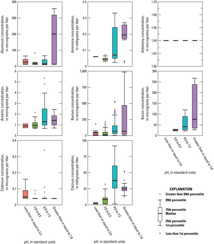
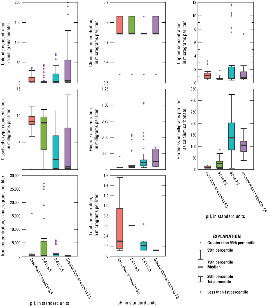
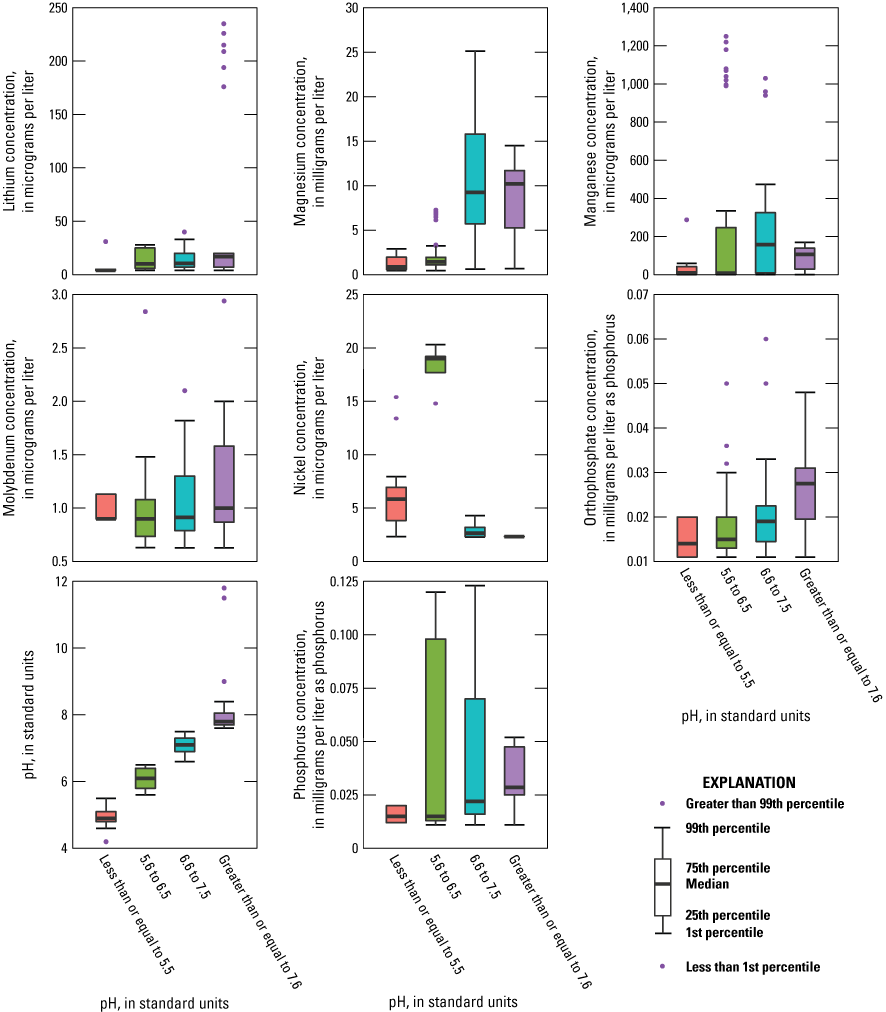
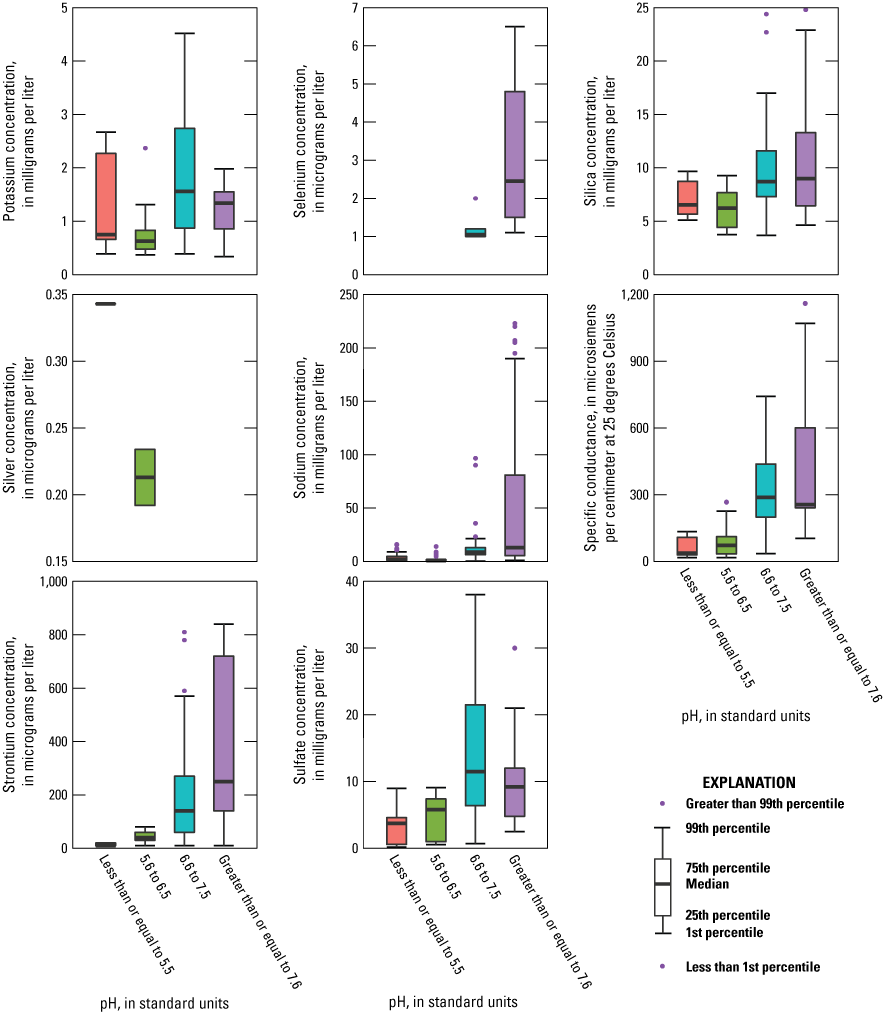
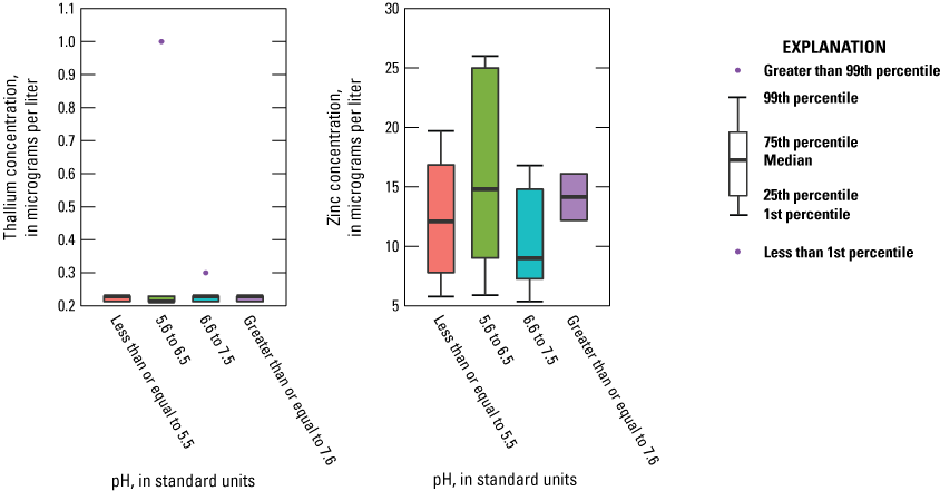
Selected constituents grouped by pH categories of ≤5.5, 5.6–6.5, 6.6–7.5, and ≥7.6 for 221 water samples collected from 28 wells within the Pennsylvania Groundwater Monitoring Network, 2015–19.
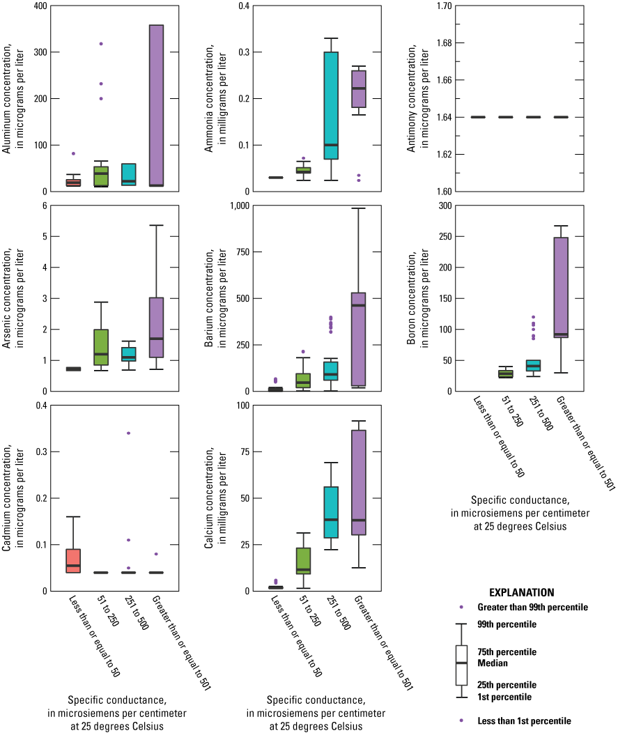
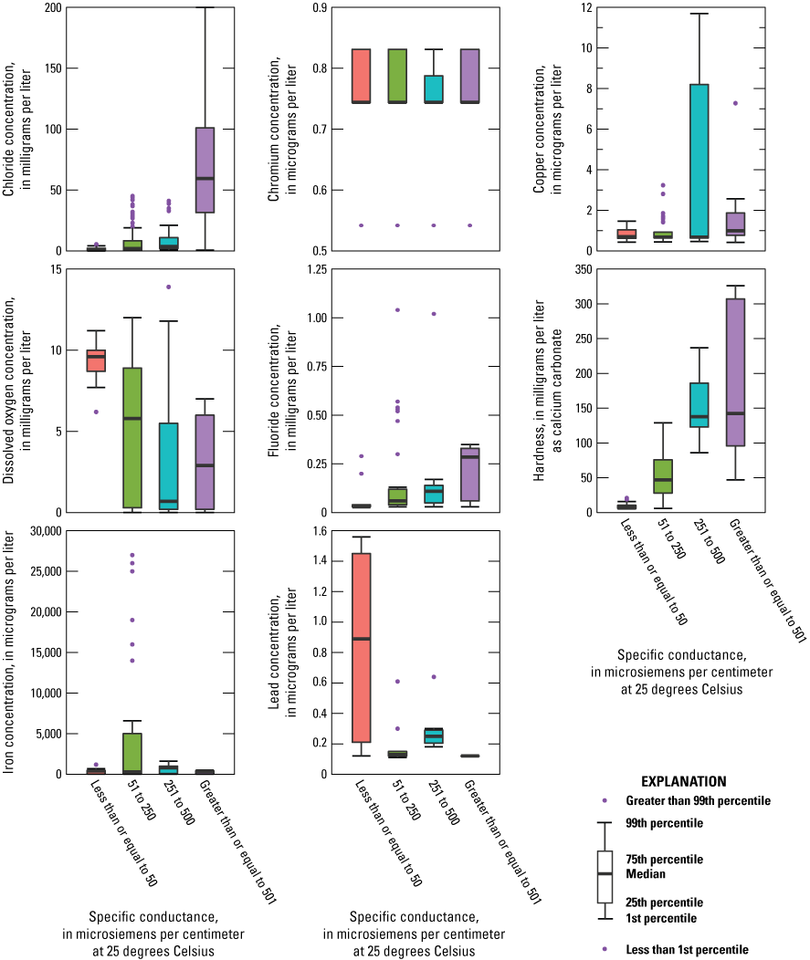
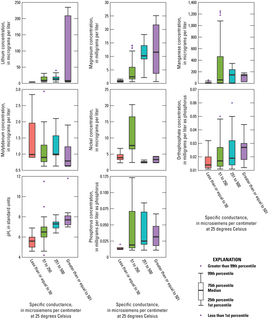
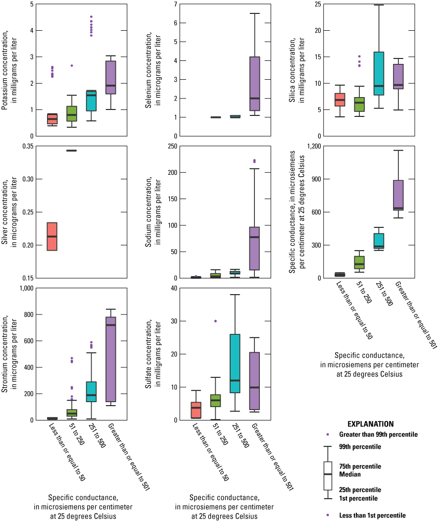
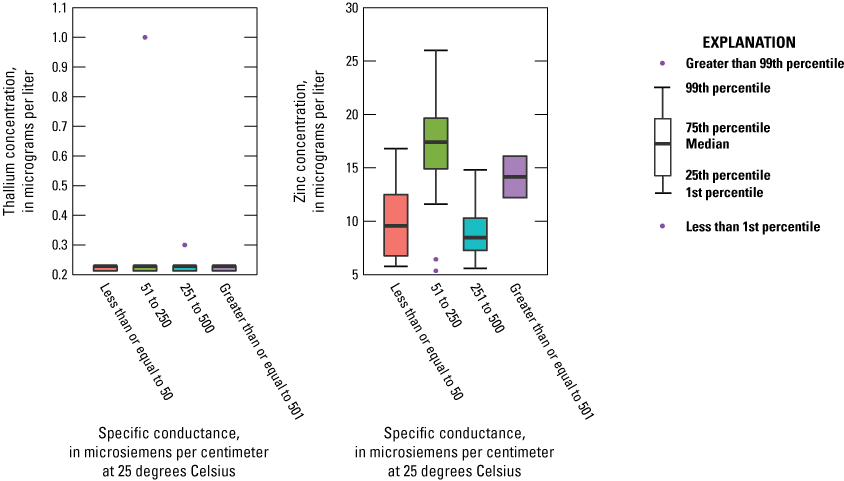
Selected constituents grouped by specific conductance categories of ≤50, 51–250, 251–500, and ≥500 for 221 water samples collected from 28 wells within the Pennsylvania Groundwater monitoring Network, 2015–19.
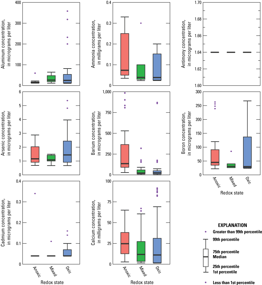
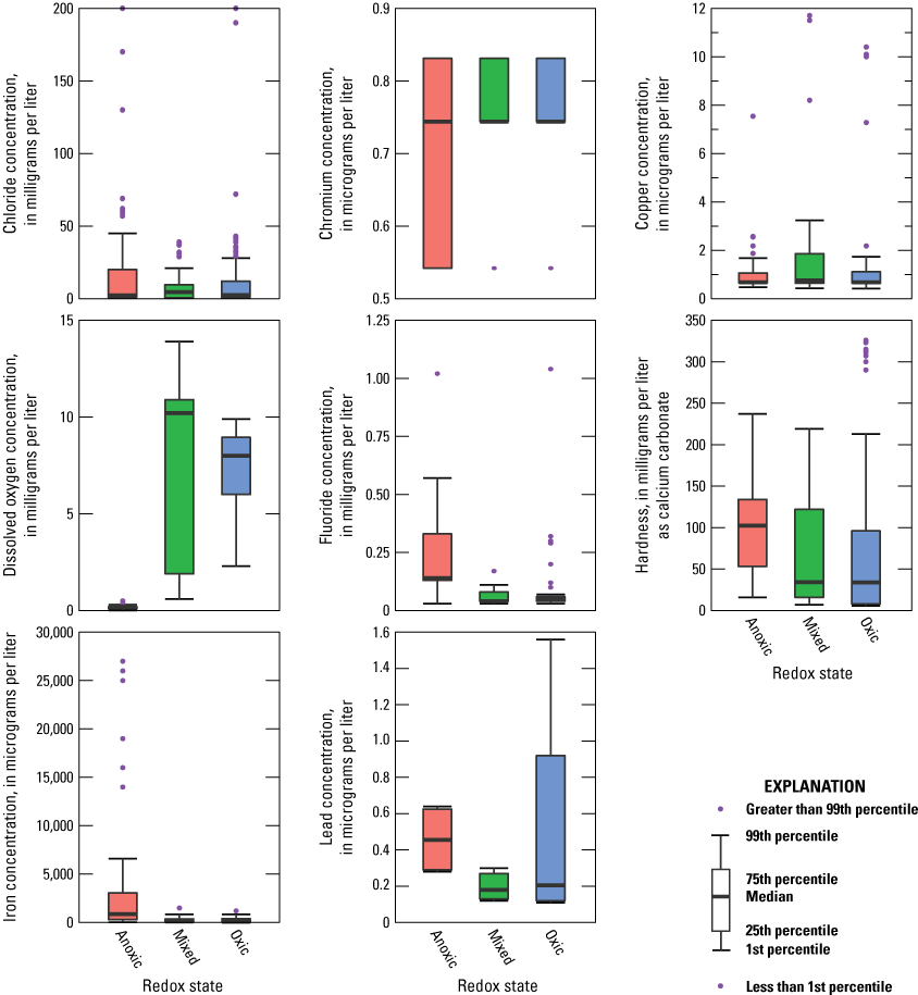
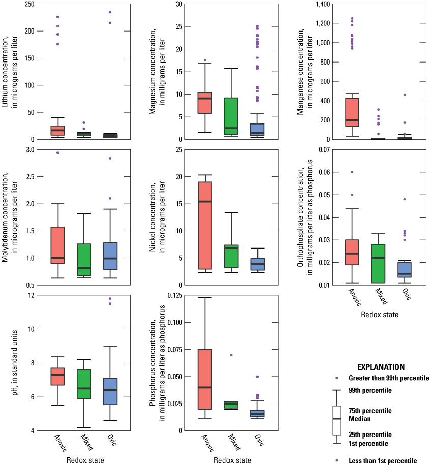
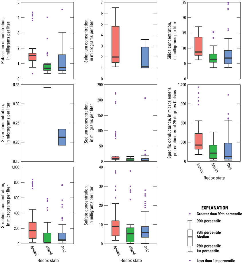
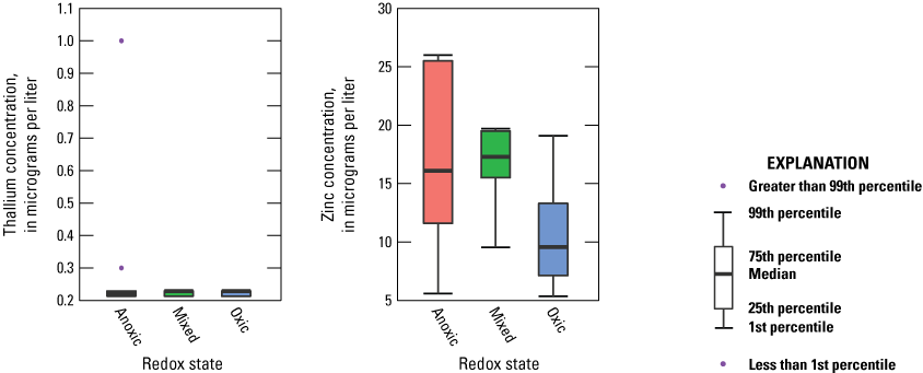
Selected constituents grouped by reduction-oxidation (redox) state categories of anoxic, mixed, and oxic for 221 water samples collected from 28 wells within the Pennsylvania Groundwater monitoring Network, 2015–19.
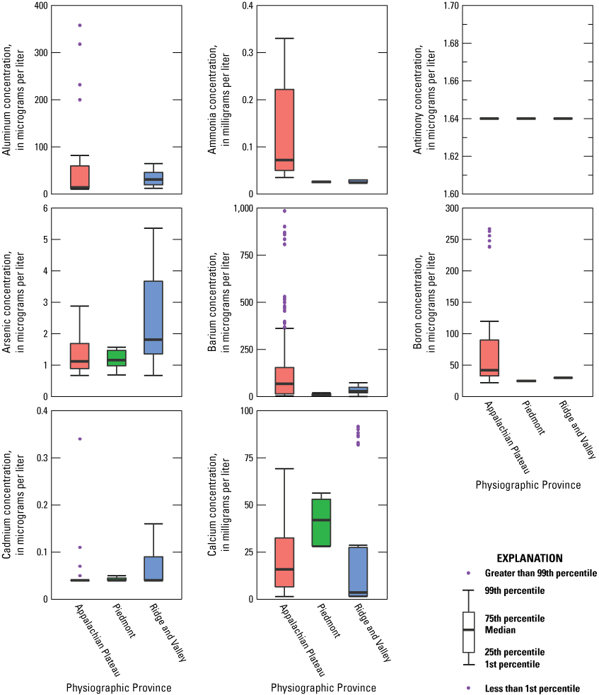
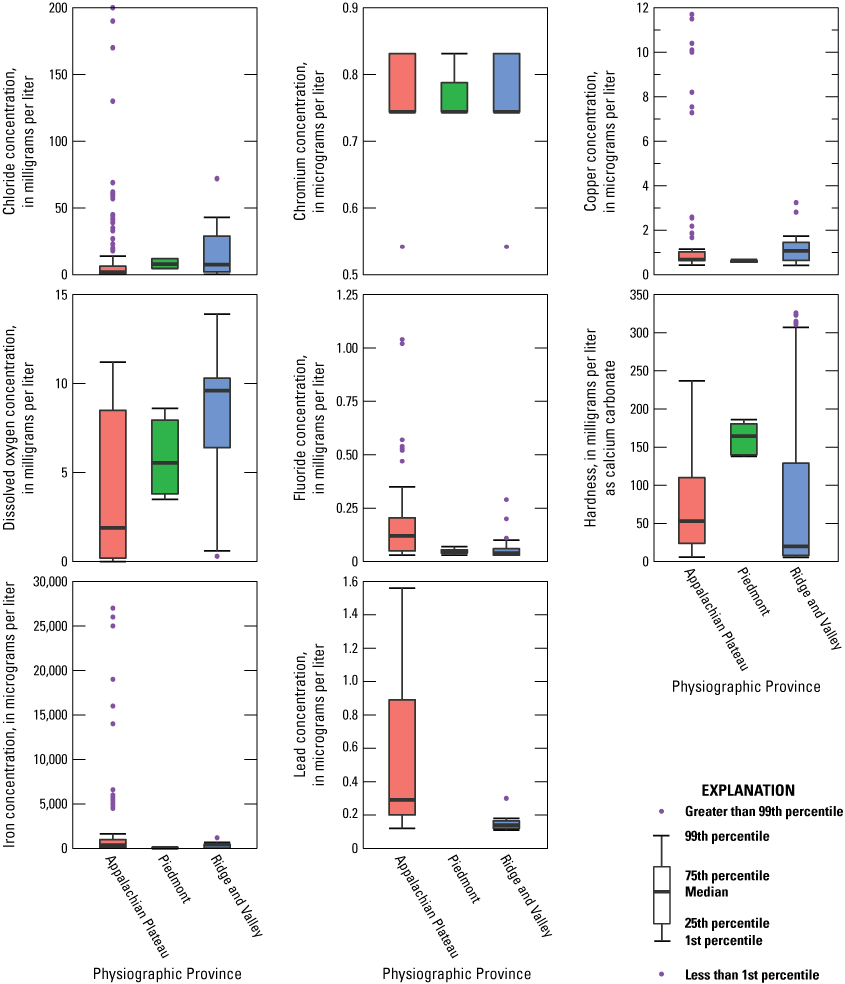
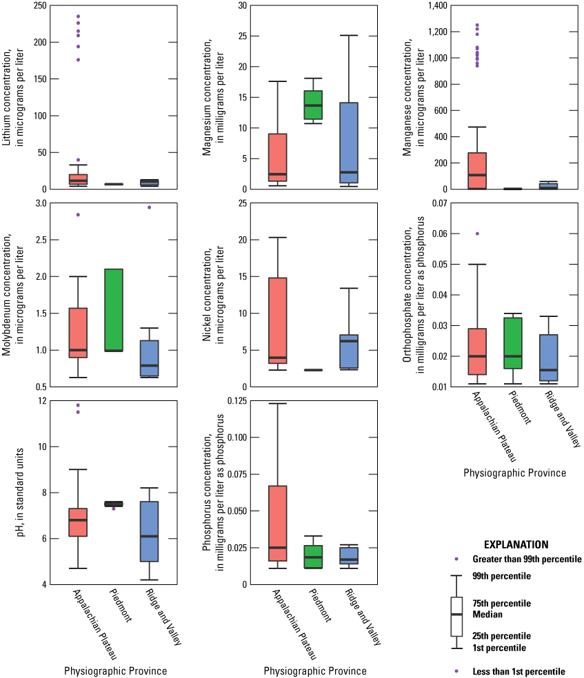
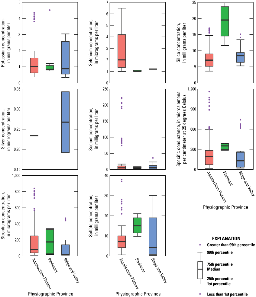
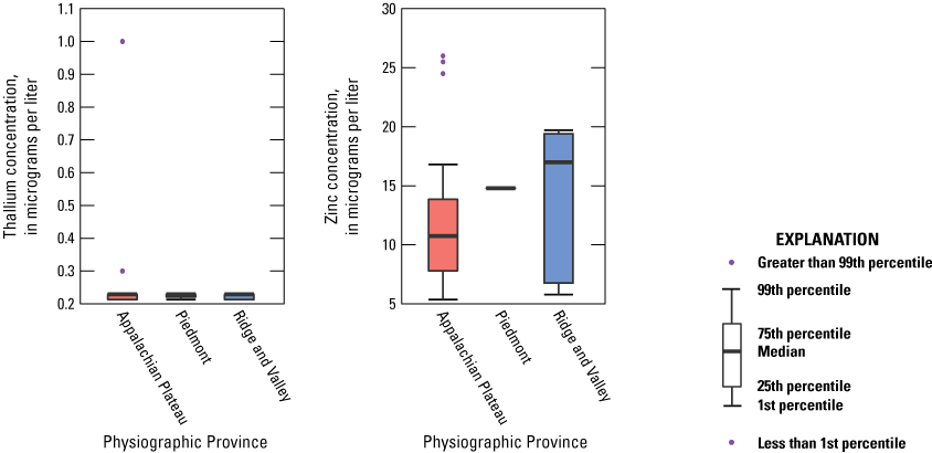
Selected constituents grouped by physiographic province categories of Appalachian Plateau, Piedmont, and Ridge and valley for 221 water samples collected from 28 wells within the Pennsylvania Groundwater monitoring Network, 2015–19.
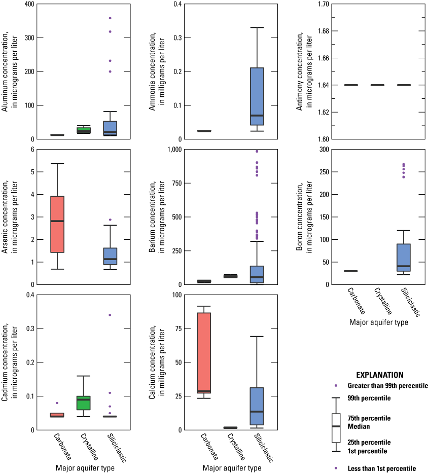
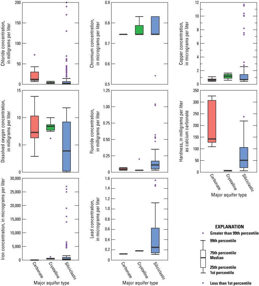
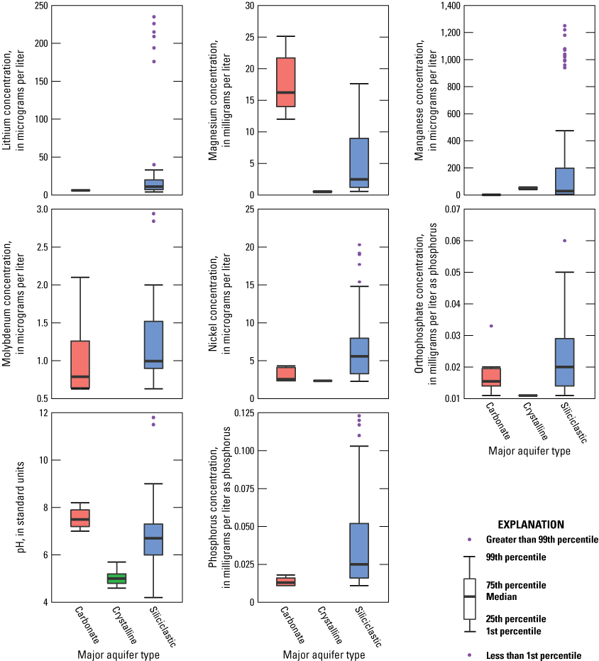
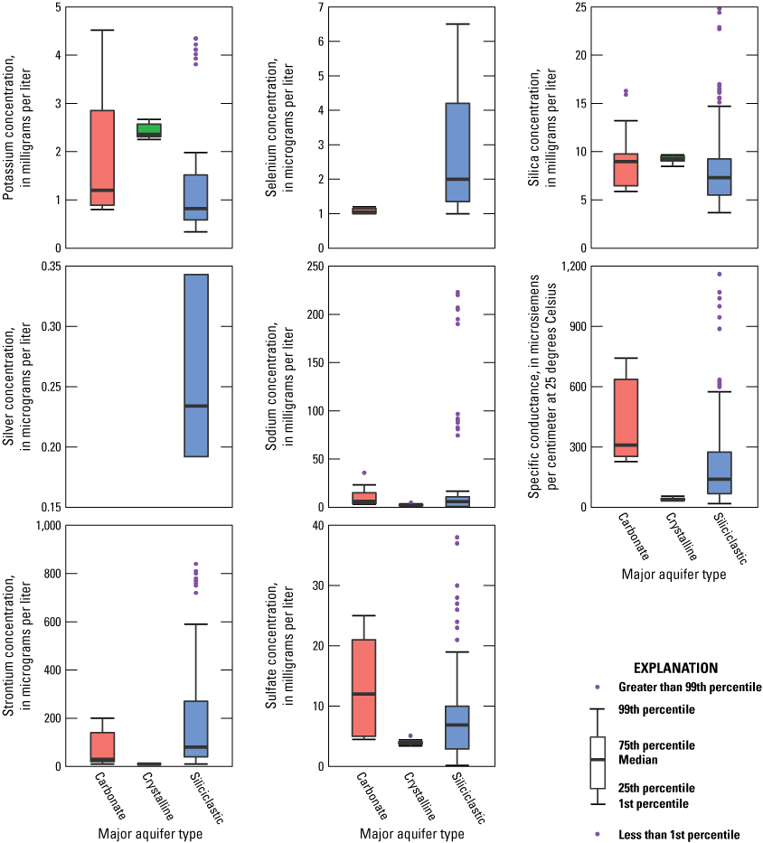
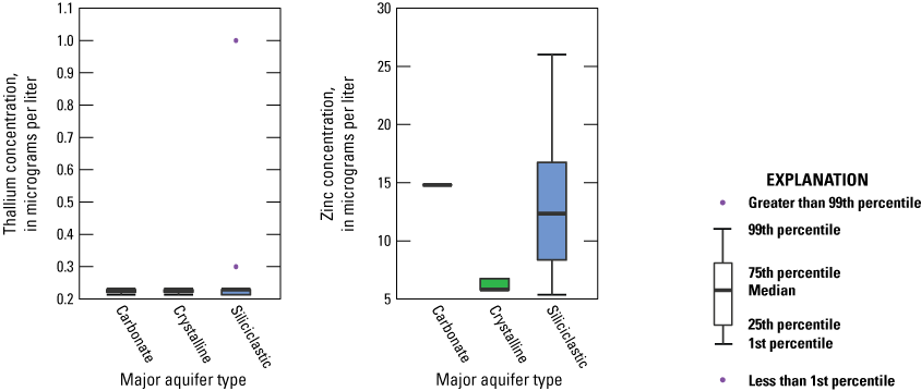
Selected constituents grouped by major aquifer type categories of carbonate, crystalline, and siliciclastic for 221 water samples collected from 28 wells within the Pennsylvania Groundwater monitoring Network, 2015–19.
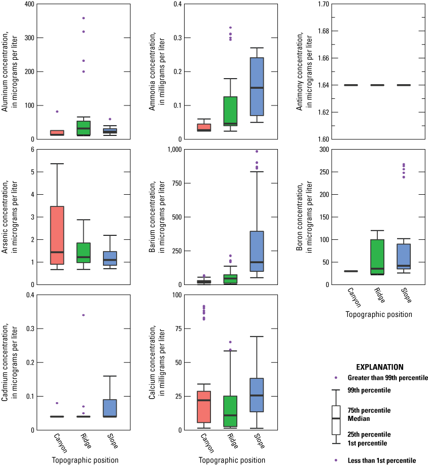
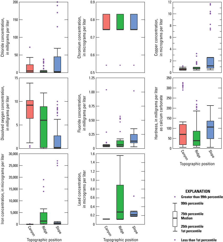
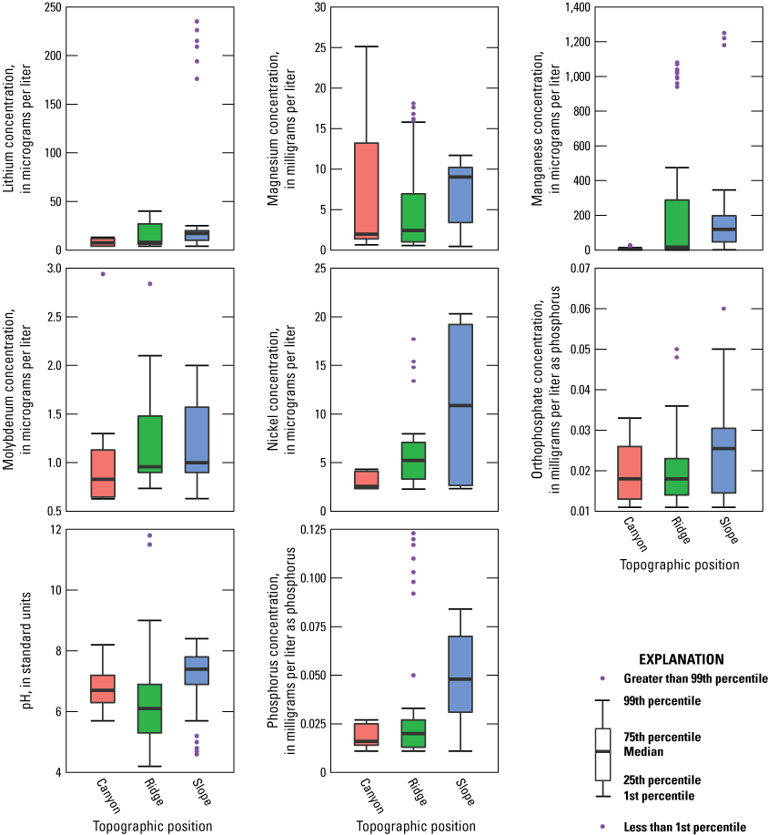
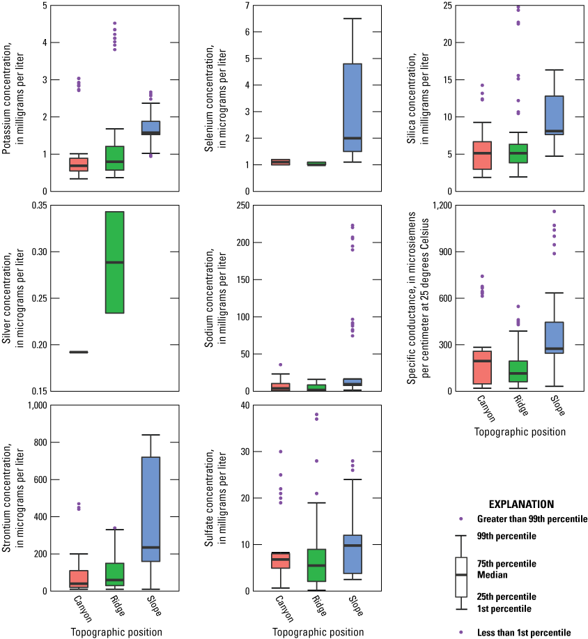
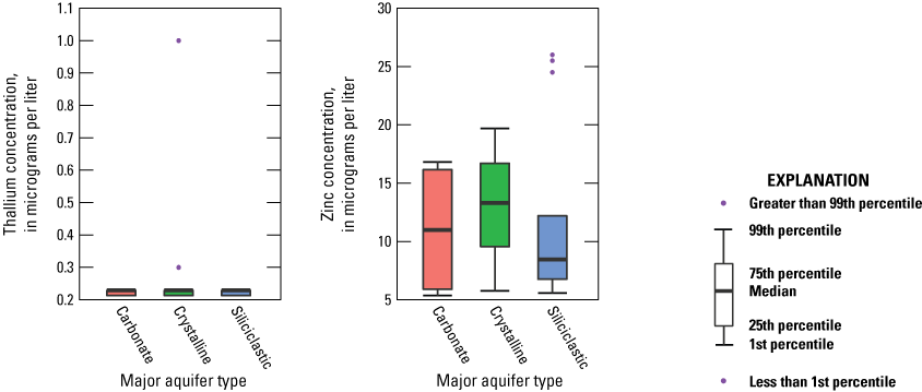
Selected constituents grouped by topographic position categories of canyon, ridge, and slope for 221 water samples collected from 28 wells within the Pennsylvania Groundwater monitoring Network, 2015–19.
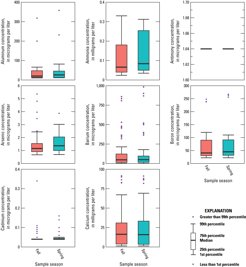
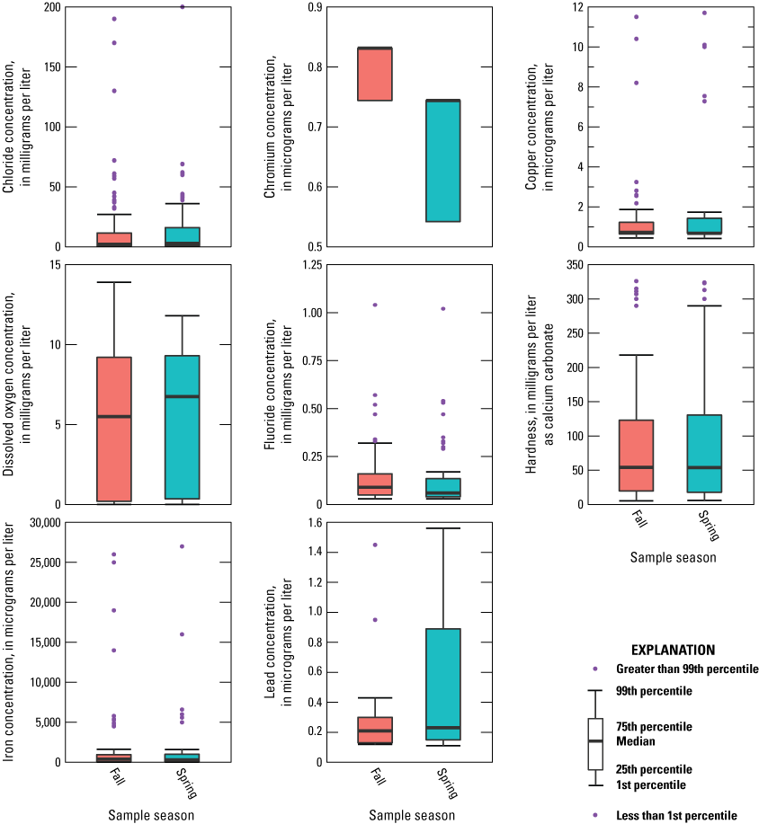
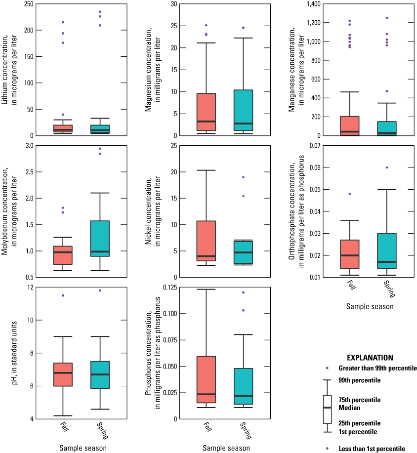
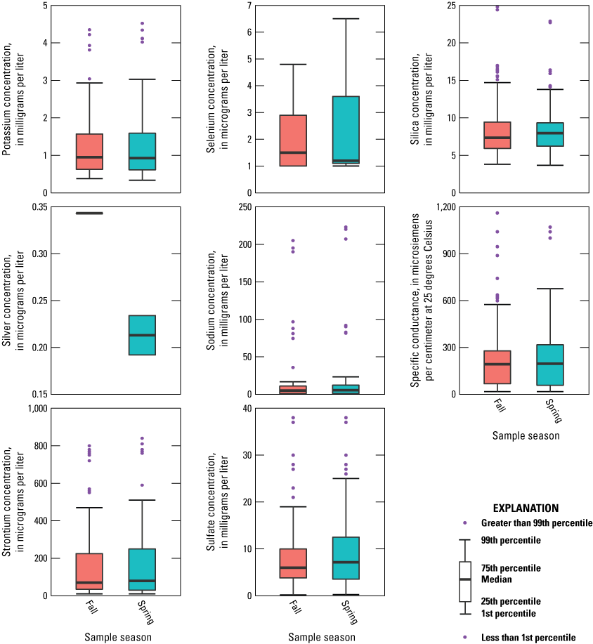
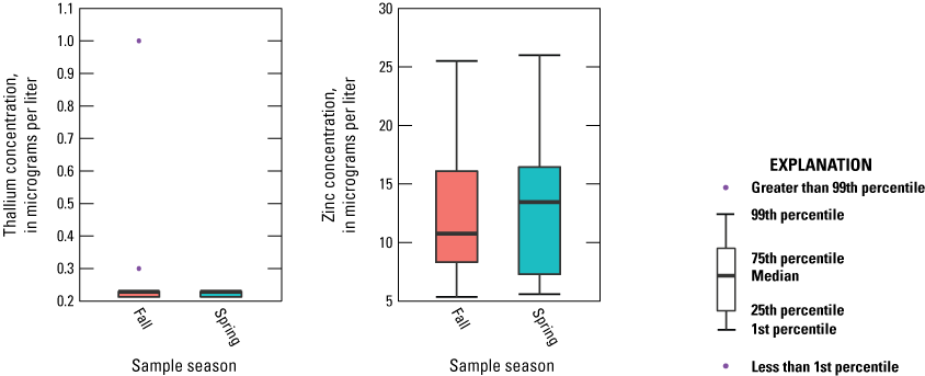
Selected constituents grouped by sample season categories of spring and fall for 221 water samples collected from 28 wells within the Pennsylvania Groundwater monitoring Network, 2015–19.
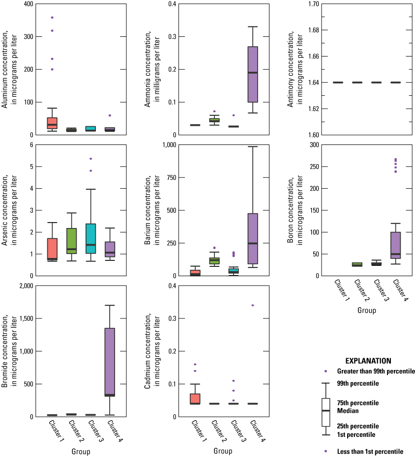
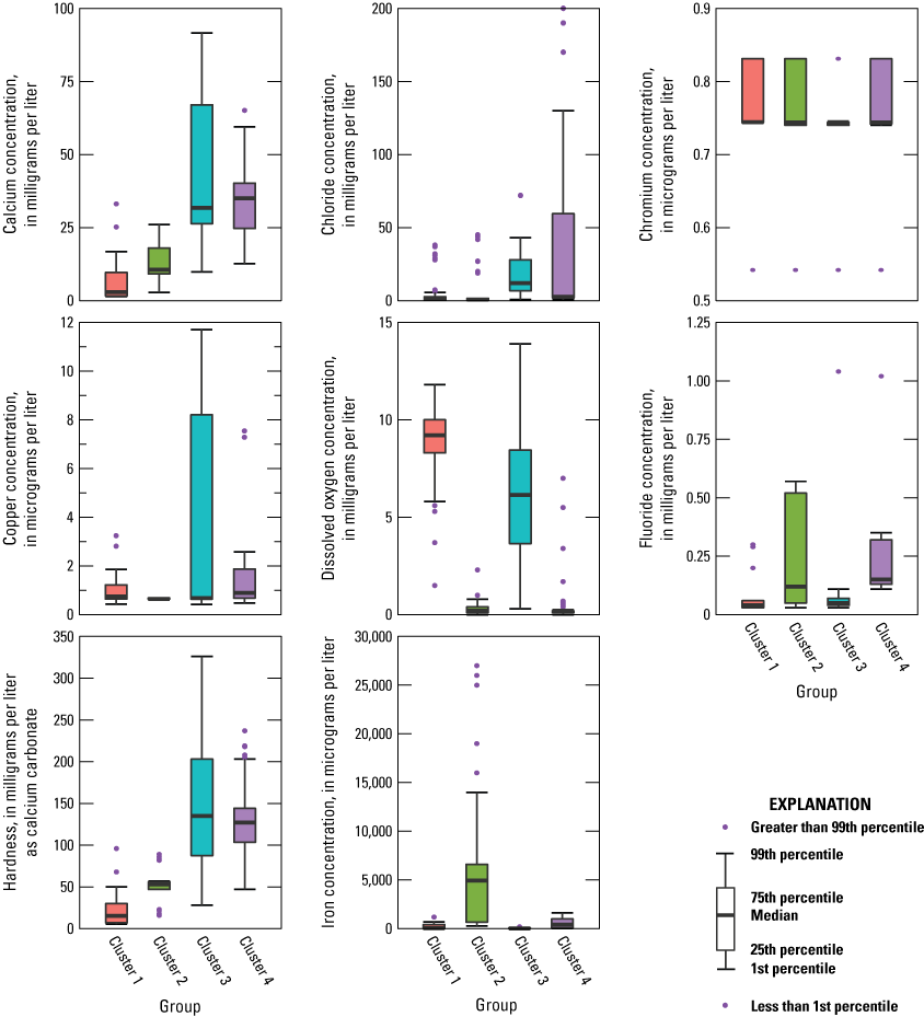
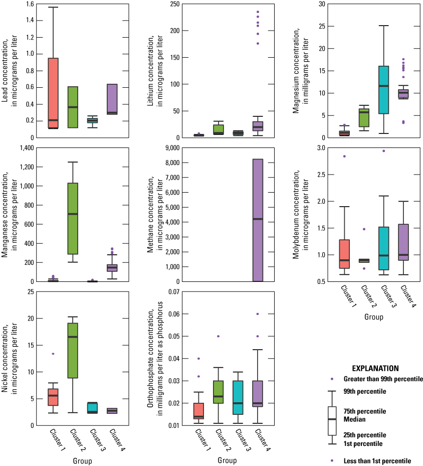
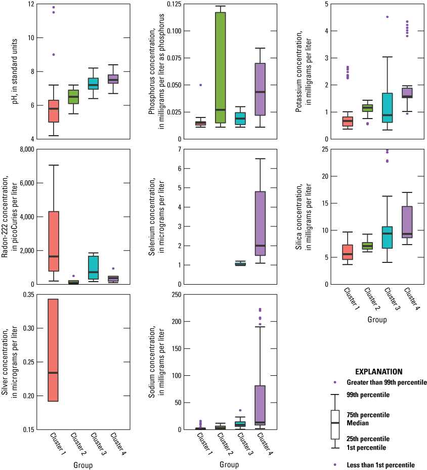
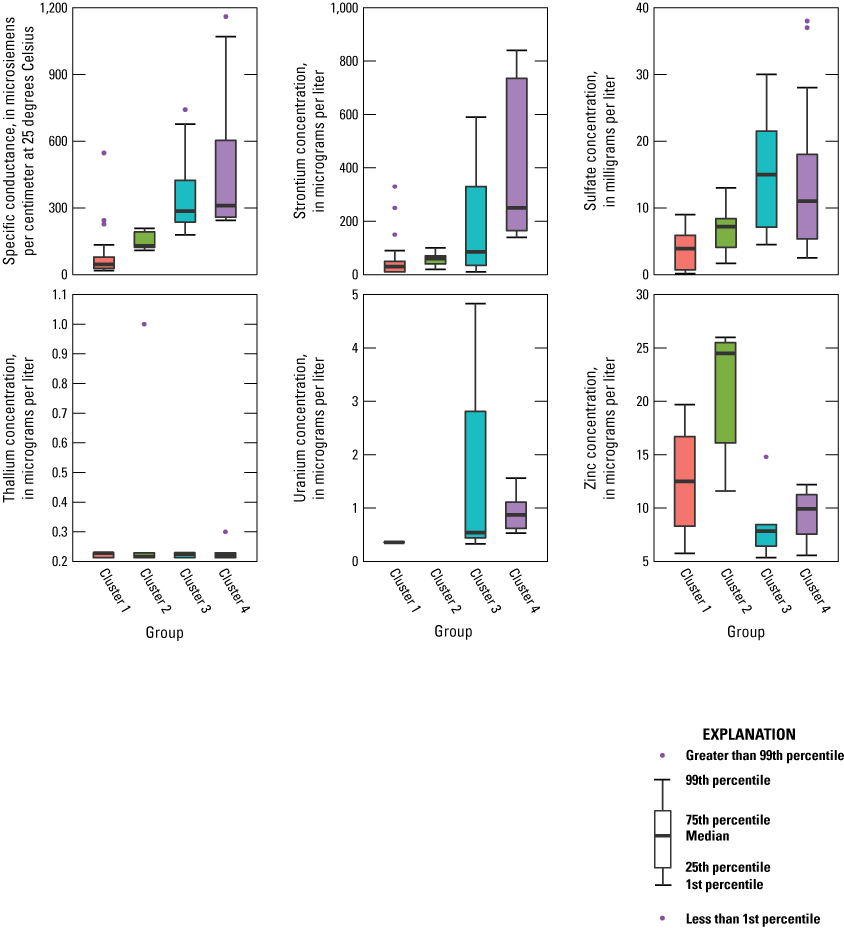
Selected constituents grouped by hierarchical cluster designation based on principal components analysis results for 221 water samples collected from 28 wells within the Pennsylvania Groundwater monitoring Network, 2015–19.
Appendix 4. Correlation matrix of selected constituents and PDSI values for Pennsylvania GWMN wells
Table 4.1.
Correlation matrix of selected constituents and time-lagged Palmer Drought Severity Index (PDSI) values for subsets of the Pennsylvania Groundwater Monitoring Network wells determined through hierarchical clustering.Appendix 5. Seasonal differences in water-quality constituents measured in selected Pennsylvania GWMN wells
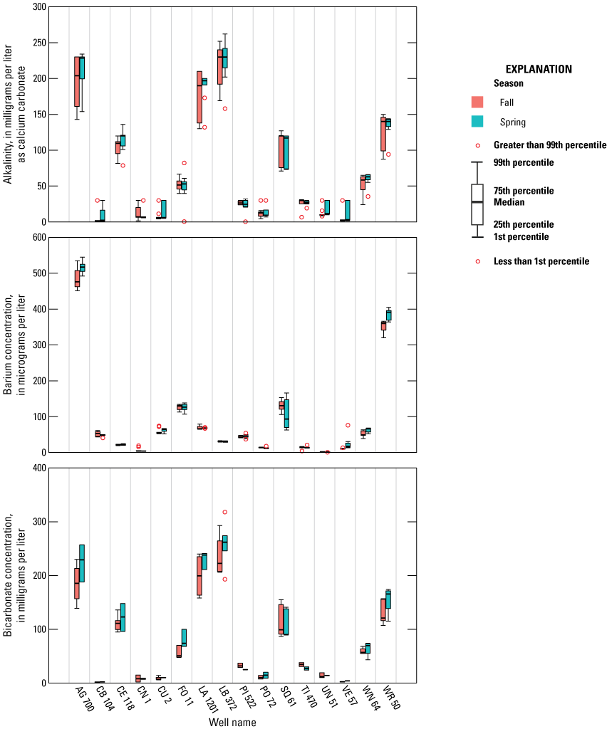
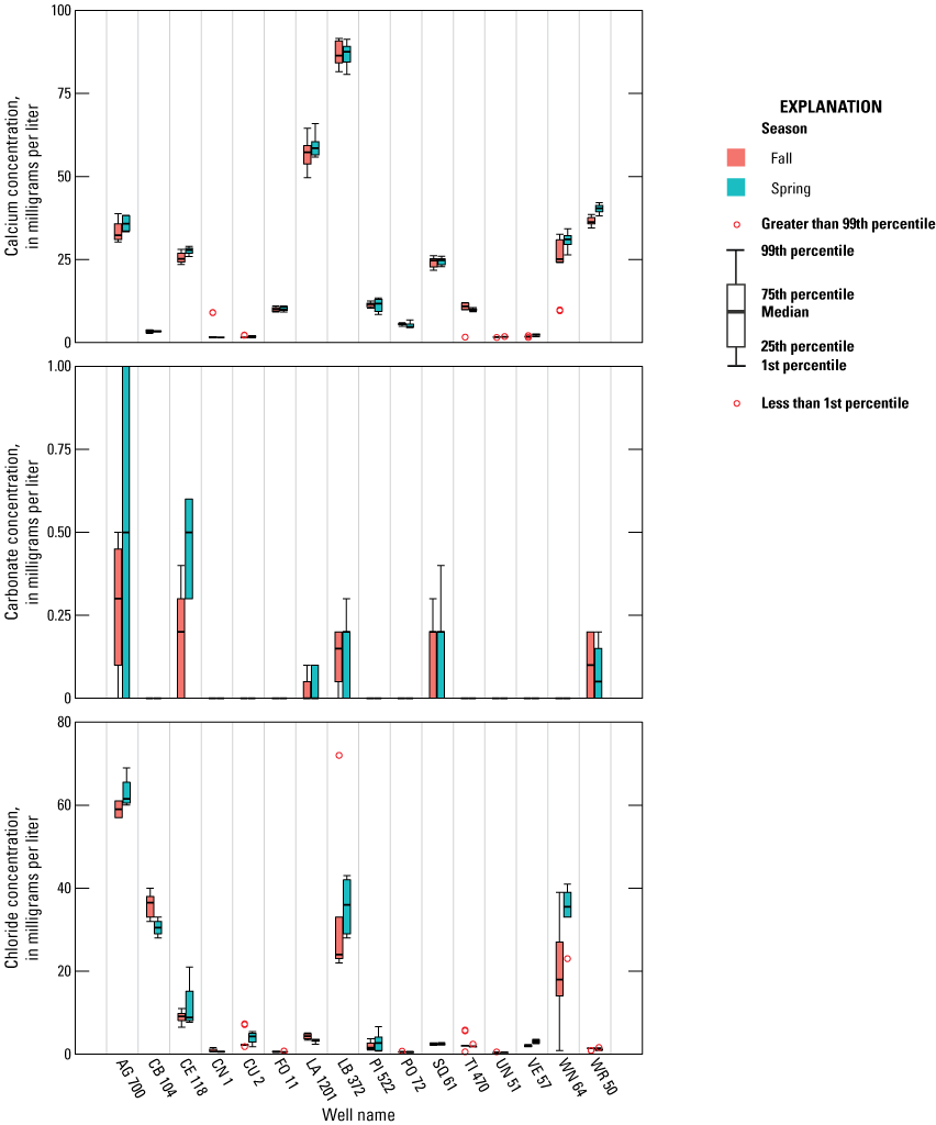
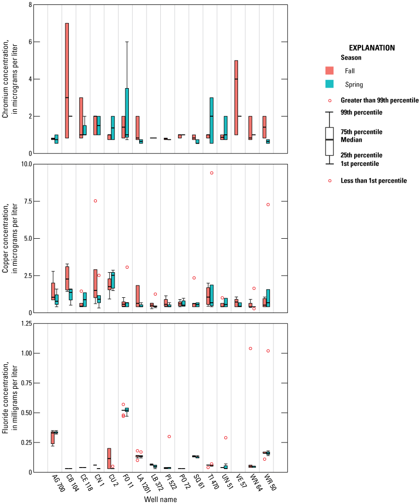
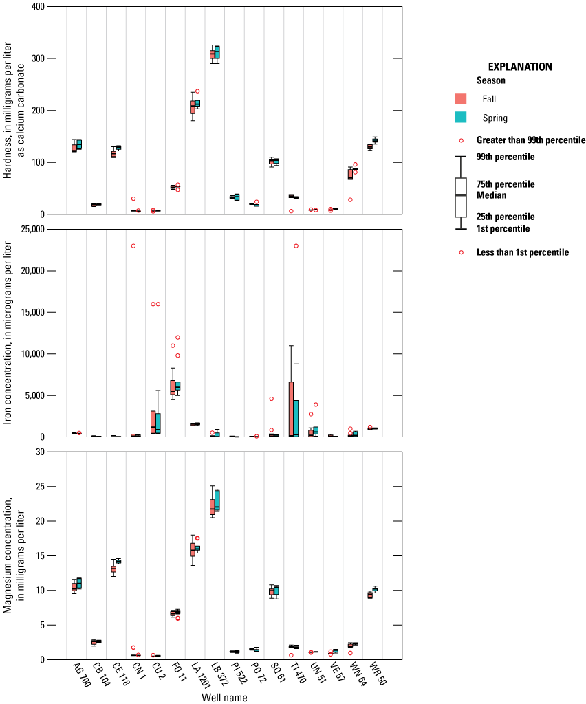
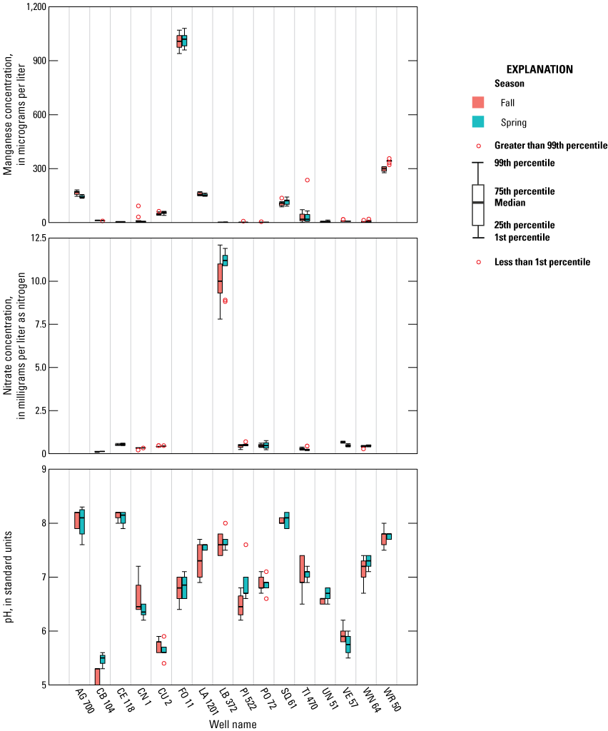
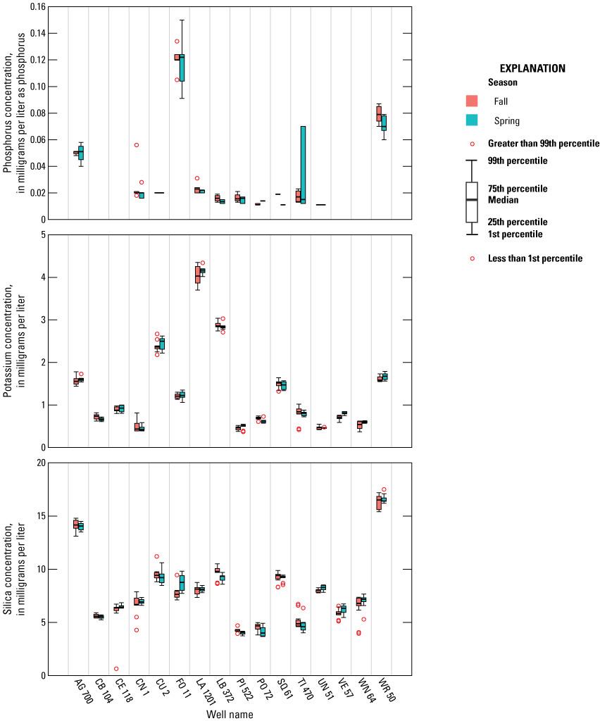
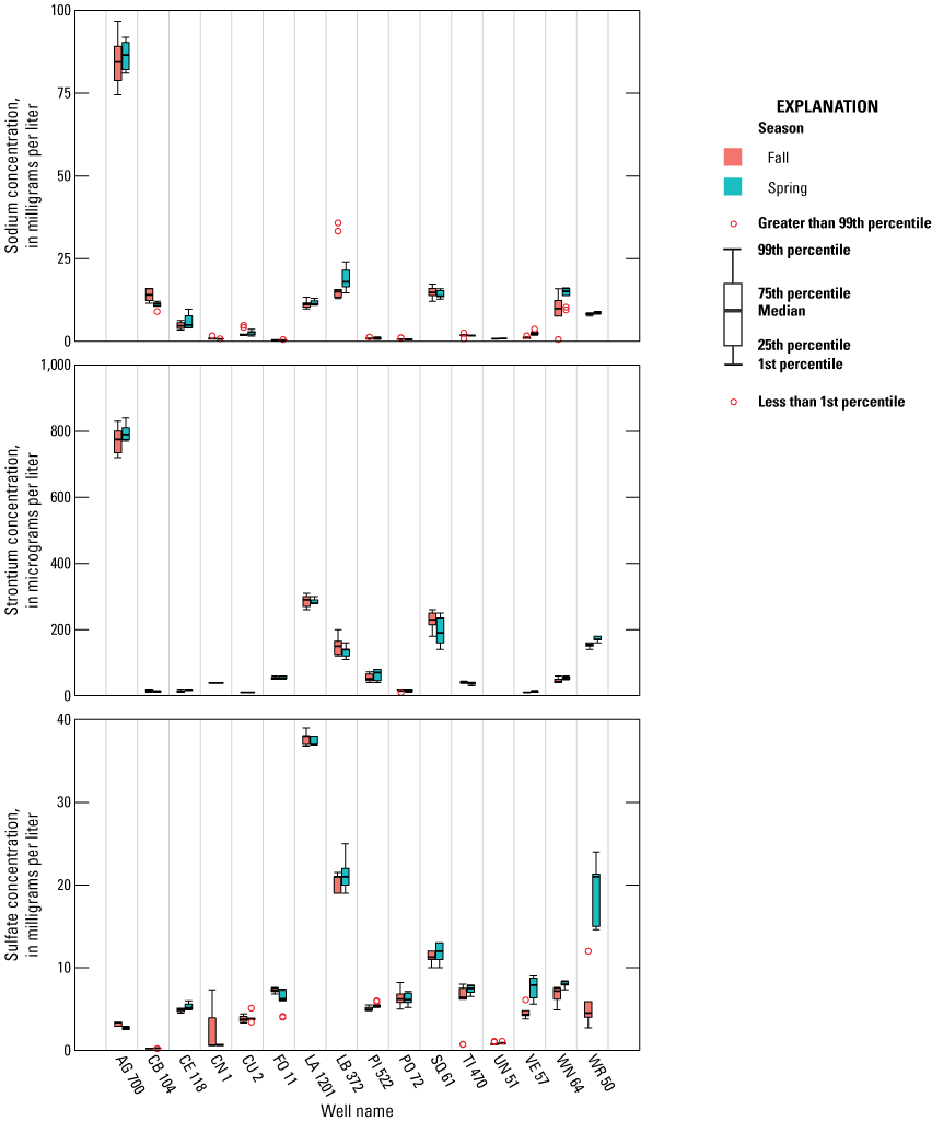
Differences in water-quality attributes from spring and fall samples, Pennsylvania Groundwater Monitoring Network, 2015–19.
Conversion Factors
U.S. customary units to International System of Units
Temperature in degrees Celsius (°C) may be converted to degrees Fahrenheit (°F) as follows: °F = (1.8 × °C) + 32.
Temperature in degrees Fahrenheit (°F) may be converted to degrees Celsius (°C) as follows: °C = (°F – 32) / 1.8.
Datum
Vertical coordinate information is referenced to the North American Vertical Datum of 1988 (NAVD 88).
Horizontal coordinate information is referenced to the North American Datum of 1983 (NAD 83).
Altitude, as used in this report, refers to distance above the vertical datum.
Supplemental Information
Specific conductance is given in microsiemens per centimeter at 25 degrees Celsius (µS/cm at 25 °C).
Concentrations of chemical constituents in water are given in either milligrams per liter (mg/L) or micrograms per liter (µg/L).
Activities for radioactive constituents in water are given in picocuries per liter (pCi/L).
Results for measurements of stable isotopes of an element (with symbol E) in water, solids, and dissolved constituents commonly are expressed as the relative difference in the ratio of the number of the less abundant isotope (ΔE) to the number of the more abundant isotope of a sample with respect to a measurement standard.
Abbreviations
°C
degrees Celsius
=
equal to
>
greater than
≥
greater than or equal to
<
less than
≤
less than or equal to
µg/L
micrograms per liter
µs/cm
microsiemens per centimeter
BOL
Bureau of Laboratories (Pennsylvania Department of Environmental Protection)
DEM
digital elevation model
DO
dissolved oxygen
DOC
dissolved organic carbon
EPA
U.S. Environmental Protection Agency
GWMN
Groundwater Monitoring Network
HAL
health advisory level
MCL
maximum contaminant level
mg/L
milligrams per liter
NAD 83
North American Datum of 1983
NAVD 88
North American Vertical Datum of 1988
NFM
National Field Manual
NGVD 29
National Geodetic Vertical Datum of 1929
NTRU
nephelometric turbidity ratio units
PaDEP
Pennsylvania Department of Environmental Protection
PC
principal component
PCA
principal components analysis
pCi/L
picocuries per liter
PDSI
Palmer Drought Severity Index
PFAS
per- and polyfluoroalkyl substances
ROE
residue on evaporation
SC
specific conductance
SMCL
secondary maximum contaminant level
TDS
total dissolved solids
USGS
U.S. Geological Survey
VOC
volatile organic compounds
For additional information, contact:
Director, Pennsylvania Water Science Center
U.S. Geological Survey
215 Limekiln Road
New Cumberland, PA 17070-2424
Or visit our website at: https://www.usgs.gov/centers/pa-water
Publishing support provided by the U.S. Geological Survey Science Publishing Network, West Trenton Publishing Service Center.
Disclaimers
Any use of trade, firm, or product names is for descriptive purposes only and does not imply endorsement by the U.S. Government.
Although this information product, for the most part, is in the public domain, it also may contain copyrighted materials as noted in the text. Permission to reproduce copyrighted items must be secured from the copyright owner.
Suggested Citation
Conlon, M.D., and Duris, J.W., 2022, Characterization of ambient groundwater quality within a statewide, fixed-station monitoring network in Pennsylvania, 2015–19: U.S. Geological Survey Scientific Investigations Report 2021–5119, 118 p., https://doi.org/10.3133/sir20215119.
ISSN: 2328-0328 (online)
Study Area
| Publication type | Report |
|---|---|
| Publication Subtype | USGS Numbered Series |
| Title | Characterization of ambient groundwater quality within a statewide, fixed-station monitoring network in Pennsylvania, 2015–19 |
| Series title | Scientific Investigations Report |
| Series number | 2021-5119 |
| DOI | 10.3133/sir20215119 |
| Publication Date | January 18, 2022 |
| Year Published | 2022 |
| Language | English |
| Publisher | U.S. Geological Survey |
| Publisher location | Reston, VA |
| Contributing office(s) | Pennsylvania Water Science Center |
| Description | Report: x, 118 p.; Data Release |
| Country | United States |
| State | Pennsylvania |
| Online Only (Y/N) | Y |
| Additional Online Files (Y/N) | N |