

Evaluation of Machine Learning Approaches for Predicting Streamflow Metrics Across the Conterminous United States
Links
- Document: Report (4.76 MB pdf) , HTML , XML
- Data Release: USGS data release - Calculated streamflow metrics for machine learning regionalization across the conterminous United States, 1950 to 2018
- NGMDB Index Page: National Geologic Map Database Index Page (html)
- Download citation as: RIS | Dublin Core
Abstract
Few regional or national scale studies have evaluated machine learning approaches for predicting streamflow metrics at ungaged locations. Most such studies are limited by the number of dimensions of the streamflow regime investigated. This study, in contrast, provides a comprehensive evaluation of the streamflow regime based on three widely available machine learning approaches (support vector regression, random forest, and cubist regression) and on multiple linear regression to predict 106 natural streamflow metrics at ungaged locations. This evaluation is done for 545 streamgages across the northwest United States for recurrence-interval flood metrics and for 1,851 sites in the conterminous United States for non-flood metrics. The results indicate that for flood metrics, predictions by cubist regression and support vector regressions have substantially less error than the other approaches. For all the remaining streamflow metrics, random forest models outperform the other methods.
Introduction
State and local water resource managers often require streamflow (hereafter referred to as flow) metrics at locations on rivers and streams that have little to no flow information. This information is often required to set regulatory limits on water use, to balance the water needs of humans with the water needs required to maintain ecosystem resources (such as fisheries and recreation), and to assist with engineering design (such as culverts). To acquire this important information, hydrologic models can be used to predict flows using statistical methods. Various statistical modeling approaches can be used for predicting flow metrics, including generalized least squares regression (Stedinger and Tasker, 1985) and a variety of machine-learning approaches (Jeong and Kim, 2005; Carlisle and others, 2016; Eng and others, 2017; Eng and others, 2019). These empirical approaches typically use basin features—such as climate, soils, and topography—to predict flow characteristics and often are applied to large geographic regions.
Machine learning approaches are now widely applied in hydrology. Machine learning approaches have been used to predict flows ranging from next day flows (for example, He and others, 2014; Lima and others, 2016) to next month flows (for example, Noori and others, 2011; Sun and others, 2014), droughts (for example, Rhee and Im, 2017), and subannual floods (for example, Mosavi and others, 2018). Although machine learning approaches are commonly used, only a few studies have been completed in which machine learning approaches are applied to predict flow metrics at ungaged locations (for example, Zakaria and Shabri, 2012; Eng and others, 2017; Peñas and others, 2018; Worland and others, 2018). Most of these studies investigated only a few dimensions of the flow regime—Zakaria and Shabri (2012) investigated flood metrics for a region in Malaysia (not shown) using support vector regression (SVR); Peñas and others (2018) investigated 16 flow metrics in a region of Spain (not shown) for generalized additive models, random forest (RF), and adaptive neuro fuzzy inference system approaches; and Worland and others (2018) focused on a low-flow metric in the southeast United States (not shown) for 8 machine learning approaches. Using only the RF approach, Eng and others (2017) comprehensively evaluated the flow regime using more than 600 flow metrics across the conterminous United States.
The objective of this study is to extend the Eng and others (2017) evaluation of RF to include three additional approaches—multiple linear regression (LR) and two other machine learning approaches (SVR and cubist regression [CR]). This study focuses on 106 flow metrics that represent various dimensions of the flow regime including three temporal scales (instantaneous, annual, and seasonal/monthly) and metrics that are associated with ecological impairment. For flood metrics, 545 streamgages in the northwest United States (fig. 1) are used to evaluate the approaches. For the remaining flow metrics, 1,851 streamgages across the conterminous United States (fig. 2) are used to evaluate the approaches.
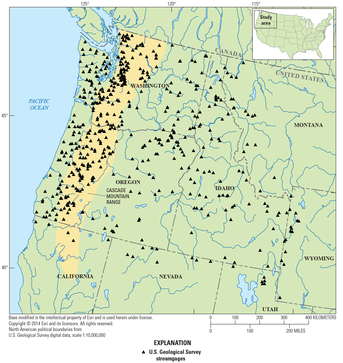
The northwest United States showing locations of 545 streamgages used to build models to predict flood flow metrics.
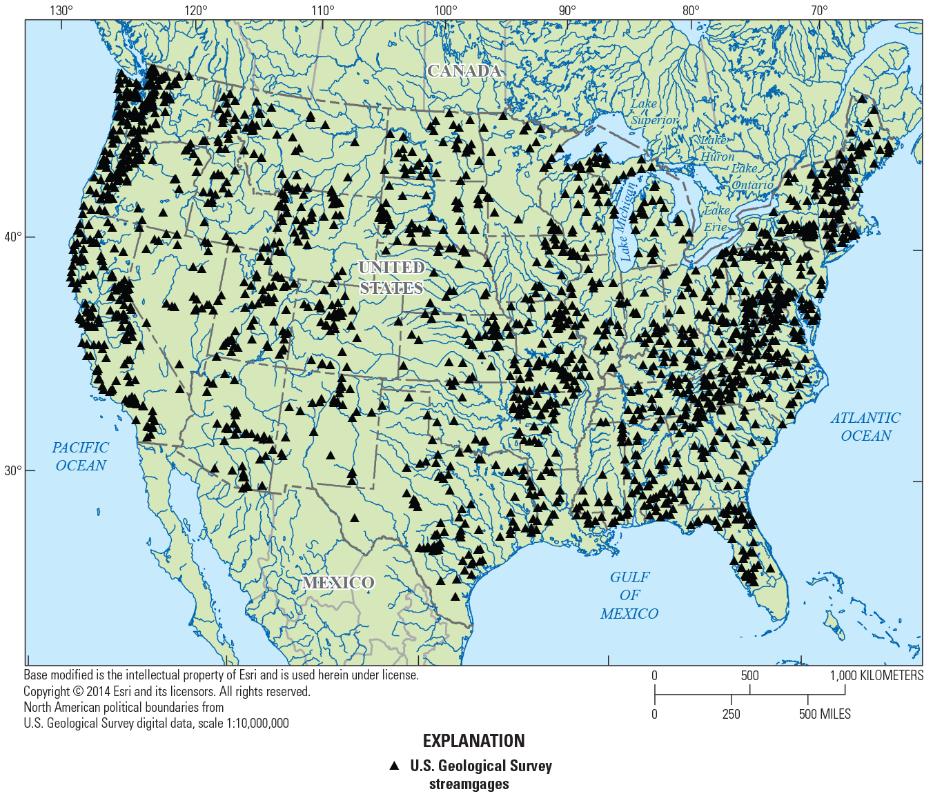
The United States showing locations of 1,851 streamgages used to build models to predict nonflood flow metrics.
Study Area and Basin Attributes
For flood metrics, 545 streamgages in Washington, Oregon, and Idaho are used (fig. 1). For the remaining flow metrics, 1,851 streamgages across the conterminous United States are used (fig. 2). These stations are a subset of about 9,000 streamgages in the Geospatial Attributes of Gages for Evaluating Streamflow II (called “GAGES II;” Falcone, 2011) database. This database contains streamgages monitoring natural (referred to as “reference”) and heavily modified (referred to as “nonreference”) basins, the latter having been affected by dams and land cover changes. Associated with each streamgage are 176 geographic information system-derived natural basin attributes calculated throughout the basin (app. 1). In summary, these attributes represent basin size and slope (n=2), climate (for example, number of days with measurable precipitation, annual and monthly precipitation, annual and monthly temperature, annual and monthly runoff, potential evapotranspiration, mean snow percentage of total precipitation, day of first freeze, and overland flow; n=64), base-flow measures (base-flow index, depth to water table, and subsurface contact time; n=3), soil properties (for example, permeability, bulk density, soil thickness, organic matter, surficial geology, chemical composition of rock, clay, silt, and sand percentages; n=87), and portion of the basin within each hydrologic landscape region (Wolock and others 2004, n=20). The annual and monthly runoff values are calculated at ungaged locations using the water balance model by Wolock and McCabe (1999), which uses precipitation and temperature information as inputs. Detailed descriptions of remaining basin attributes and source data are provided by Falcone (2011). Basin attributes potentially affected by direct human modifications, such as land use, vegetation (nonnative), and open water, were not considered as predictors. The 176 basin attributes are used as predictor variables in machine learning and LR approaches to predict flow metrics in this study (Falcone, 2011; Eng and others, 2017).
Methods
This section describes the methods used in the evaluation of LR and machine learning approaches for predicting flow metrics. The selection and calculation of flow metrics and a brief description of LR and machine learning approaches also are discussed in this section.
Flow Metrics
Selection of the 106 flow metrics includes 6 flow metrics that are ecologically relevant (Carlisle and others, 2017; Eng and others, 2019) and an additional 100 flow metrics chosen from the StreamStats (Ries and others, 2017) database (table 1). The 106 flow metrics consist of “interpretive” and “noninterpretive” measures of flow dimensions; interpretive flow metrics require subjective hydrologic judgement, such as fitting parametric distributions and removing outliers from data. Noninterpretive metrics do not require subjective judgement and include metrics such as the arithmetic mean or coefficient of variation. This list of 106 metrics represents flow metrics that State and local water resource managers need in order to predict conditions at ungaged locations. Each flow metric and a brief description are listed in table 1. To simplify the results and discussion of these flow metrics, the metrics are grouped into three types based on time frames—flood metrics, annual flow metrics, and seasonal/monthly flow metrics.
Table 1.
The 106 flow metrics assessed in this study.[DA, drainage area; P10, 10-percent nonexceedance flow; P90, 90-percent nonexceedance flow]
The flow metric was determined to be associated with ecological impairment by Carlisle and others (2017).
Recurrence interval flood values (2-, 5-, 10-, 25-, 50-, 100-, and 500-year) are considered interpretative flow metrics because the flood values are calculated using Bulletin 17C (England and others, 2019) procedures, which involves fitting log Pearson Type III distributions to annual time series of instantaneous maximum flow values. In addition, prediction of the flood values requires development of a regional skew estimator (for example, Veilleux and others, 2011). Because of the interpretive nature of these factors, this study only uses previously determined recurrence interval flood values from published flood studies. All recurrence interval flood values are taken from flood studies in Washington, Oregon, and Idaho (Cooper, 2005; Mastin and others, 2016; Wood and others, 2016). For some basins, Wood and others (2016) derived flood values from basins that have undergone human modifications by only analyzing periods of record not affected by those human impacts. This region was chosen because a regional skew map for the northwest United States is available (Wood and others, 2016, app. B). The flood metrics are log (base 10) transformed before being used to form models (for example, Thomas and Benson, 1970).
The remaining flow metrics are noninterpretive and are calculated across the conterminous United States for 1950–2018. Methods outlined in Eng and others (2017) and Eng and others (2019) are used to calculate all nonflood flow metrics (except the monthly nonexceedance metrics) in this study. The monthly nonexceedance metrics are calculated by first taking all daily flow values for the month of interest in all years during 1950–2018. Months with missing daily flow values are excluded from analysis. These values are then ranked in descending order, and the flow values associated with 10, 20, 50, 80, and 90 percent of all flow values are assigned as the monthly nonexceedance values. Every magnitude-related flow metric (except flood metrics), such as mean flows, is normalized by drainage area to improve the predictability (for example, increasing the Nash-Sutcliffe Efficiency and reducing the percent bias) of these metrics (Eng and others, 2017). The flood metrics are log (base 10) transformed and are not normalized by drainage area in order to minimize bias. All noninterpretive flow metrics are available in an associated data release (Eng, 2022).
Linear Regression and Machine Learning Approaches
The purpose of this study is to evaluate the performance of three primary types of machine learning that are widely available to the public in different programming languages as well as LR. The three types of machine learning approaches are RF, epsilon SVR, and CR. In this study, the R programming language “randomForest” package (Liaw and Wiener, 2018) is used for RF, the SVR “e1071” package (Meyer and others, 2019) is used for SVR, and the “Cubist” package (Kuhn and others, 2020a) is used for CR.
RF is an ensemble classification and regression tree (CART) method (Breiman, 2001). A conceptual diagram of RF is shown in figure 3A. RF models typically are formed from hundreds to thousands of individual “trees.” For each tree, a random subset of predictor variables and associated predictands is selected to form the model. “Splits” are used to group the observations into two separate collections, and these splits are determined based on a randomly selected subset of predictors. These groups of observations are referred to as a “node.” Predictions from this model are calculated using a subset of data not chosen for model training (also known as out-of-bag). Thus, a prediction is made by inputting the independent variables through each tree (fig. 3A). Each tree results in a single prediction either by averaging the observations (regression) or by selecting the highest frequency class (classification) in the terminal nodes. The final prediction is calculated as the average of all predictions from every tree if using a RF regression. For RF classification, each tree results in a predicted class and the highest frequency (“votes”) of the predicted class among all trees is reported as the final class prediction.
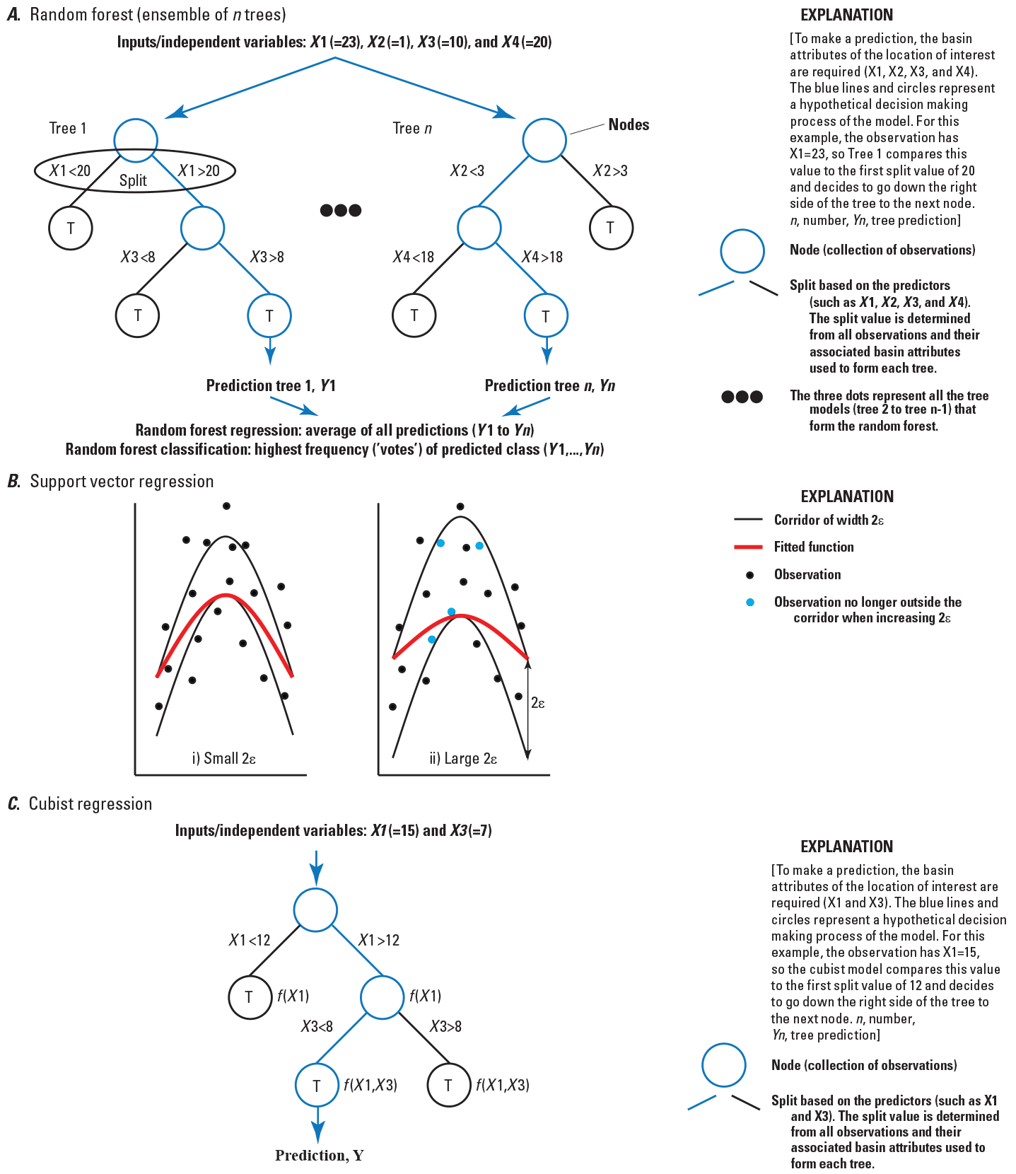
Conceptual diagram of A, random forest; B, support vector regression; and C, cubist regression.
SVR fits a function within a “corridor” defined in predictor-variable space (Vapnik, 1995). A conceptual diagram (fig. 3B) is shown to help understand how SVR fits functions. The width of the corridor, 2ε, is defined by the user, and this width substantially affects how the function fits the observations; larger width corridors (fig. 3B, right panel) fit functions that are more robust and less affected by swings in the observations compared to smaller width corridors (fig. 3B, left panel). The following two constraints are used on the placement of the function: (1) minimizing the function’s curvature within the corridor and (2) minimizing the deviations from the function to observations outside of the corridor (Smola and Schölkopf, 2004).
CR is a hybrid of CART and regression (Quinlan, 1992; Quinlan, 1993a; Quinlan 1993b; Kuhn and others, 2020a). A conceptual diagram of CR is shown in figure 3C. Similar to CART, a tree is formed by successive splitting of the observations based on a selected predictor variable. Each split terminates in a node and CR fits a function (LR is used in this study), using all predictors that are used in all splits above the node to make predictions. The final prediction is obtained from the regressions in the terminal nodes, which are adjusted based on the preceding nodes regression. The CR tree is then simplified to a set of if-then rules to determine when to apply the LRs.
The datasets containing 545 and 1,851 streamgages are each split into a calibration and cross-validation dataset. The calibration dataset is formed from 90 percent of the total number of streamgages, and the remaining 10 percent are used as a cross-validation dataset. This process of creating calibration and cross-validation datasets is repeated 100 times using random selection of sites for the calibration and cross-validation datasets.
For RF, the methods from Eng and others (2017) are used in this study. To summarize, initial RF models are formed using all 176 basin attributes as predictors for each flow metric to determine the most influential predictors based on the importance measure by Friedman (2001). From these initial models, the top 20 predictors are identified and a final model is formed using only these 20 predictors for each flow metric. The value of 20 is subjectively chosen to increase the probability that only influential basin attributes are chosen at each split for all the trees that form the forest, so that trees using noninfluential basin attributes are reduced. The tuning parameters for the SVR and CR are optimized using the caret R package (Kuhn and others, 2020b).
A back-stepwise LR, stepAIC function in the R language package MASS (Ripley and others, 2020), is used in this study to provide the baseline for comparison. This method can result in selection of more than one dozen predictor variables, which leads to overfit models. The number of predictors to include in a linear regression can be determined from previous studies (for example, Jennings and others, 1994; Lombard, 2004; Wilkowske and others, 2008; Dudley, 2015); for a variety of flow characteristics, the number of predictors in linear regressions often does not exceed five. The top five basin attributes identified by the stepAIC function are used in this study.
Performance of all methods is based on 100 bootstrapped cross-validation test datasets. For all flow metrics, a composite performance metric (CPM) is used (Eng and others, 2017). In the composite approach, performance is measured based on a normalized sum of four weakly correlated (Pearson correlation less than 0.3) performance measures—Nash-Sutcliffe Efficiency (Nash and Sutcliffe, 1970), percent bias (Gupta and others, 1999), mean of the observed values divided by predicted values (Carlisle and others, 2010), and the standard deviation of observed values divided by predicted values (Carlisle and others, 2010). Each performance measure is normalized to a value from 0 to 0.25 and summed, so that the total CPM score varies between 0 and 1, where a higher CPM score indicates better performance.
For flood metrics, the root mean square error (RMSE, Aitchison and Brown, 1957) also is reported in this study in addition to the CPM because the RMSE is of primary interest to end users (Jennings and others, 1994). The RMSE value is expressed as a percentage of the observed value as follows:
where whereN
is the total number of residuals for all bootstraps,
QT
is the observed T-year flood metric, and
is the predicted T-year flood metric.
The LR, SVR, RF, and CR methods identify specific drivers that are the most statistically significant predictors related to flow metrics. To generalize these relations, flow metrics and predictors are grouped into similar types. The flow metrics are grouped according to the following categories: (1) magnitude flow metrics are grouped into low (1-, 7-, and 30-day consecutive minimum flows; and 1-, 10-, and 25-percent nonexceedance flows), high (75-, 80-, 90-, and 99-percent nonexceedance flows), and mean (average daily flow and 50-percent nonexceedance flow) (miscellaneous metrics [such as rises] and groups consisting of less than three metrics are excluded for simplicity) in each of the flood, annual flow, and monthly flow metrics categories; and (2) monthly flow metrics and predictors are generalized by season (winter [November, December, and January]; spring [February, March, and April]; summer [May, June, and July]; and fall [August, September, and October]).
The predictors are generalized by identifying the top three predictors for the best performing method for each flow metric. For LR, the predictors associated with the lowest p-values are selected. For RF, top predictors are identified by the largest reductions in the mean square error for the model that results when these predictors are included in the models. Lastly, the R caret package (Kuhn and others, 2020b) is used for CR and SVR to determine the top predictors. The top three predictors are identified for each method in each bootstrap. The predictors that have the highest frequency for all bootstraps are chosen as the most statistically significant predictors. These predictors are generalized by type (specifically, basin feature (drainage area [DA] and slope), runoff, precipitation, temperature, base flow, and soils). Lastly, all predictors that are significant in more than one-half of the models for each generalized flow group (for example, winter low flows) are retained.
To examine the relation of significant predictors to the predictand, partial dependency plots are used. These plots indicate how the predictand varies as the predictor of interest is changed, while holding the other predictors constant. These relations can indicate nonlinear increases, decreases, and invariant behaviors over different ranges of the predictor variable. The partial dependency plot “pdp” R programming package is used in this study (Greenwell, 2018).
Performance Evaluation
The evaluation of machine learning and LR are described in this section. First, the evaluation of approaches for flood metrics at 545 streamgages in the northwest United States is described. Second, the evaluation of approaches for annual flow metrics at 1,851 streamgages across the conterminous United States is described. Lastly, the evaluation of approaches for seasonal and monthly flow metrics at 1,851 streamgages is provided.
Flood Metrics
CR and SVR result in the lowest RMSE values for all recurrence intervals (fig. 4, top panel) for flood metrics. In general, LR is associated with the poorest performance. CR and SVR result in about 20- to 30-percent reductions in the RMSE values when compared to LR. Examination of the observed flood metrics compared to the predicted metrics shows that RF is underpredicting the largest values and overpredicting the smallest flood values, whereas the other approaches do not share this problem (fig. 5). Figure 5 shows that the predicted values for the CR and SVR approaches are more precise than for the other approaches over the entire range of observed values. The vertical “banding” feature (fig. 5) illustrates the variability in the predicted metrics because of the bootstrapping procedure used for creating cross-validation datasets.
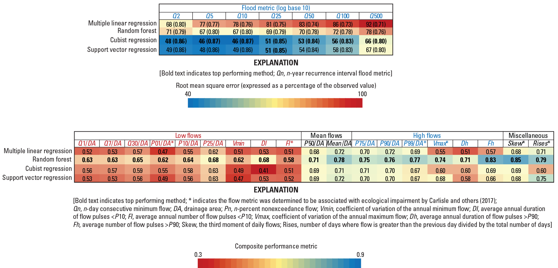
Root mean square error and composite performance metric values (values in parentheses) for flood (top panel) and annual flow metrics (bottom panel).
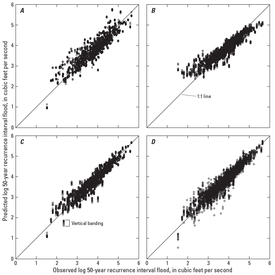
Observed versus predicted log 50-year recurrence interval flood. A, multiple linear regression; B, random forest; C, support vector regression; and D, cubist regression.
For all flood metrics, the top predictors for the CR method are log (base 10) transformed drainage area, winter precipitation, and winter runoff values (Wolock and McCabe, 1999) with base-flow index being used often in rule sets (table 2).
Table 2.
Significant generalized predictors for the best performing method (cubist regression for flood flow metrics and random forest for nonflood flow metrics).[X, statistically significant predictor; DA, drainage area; W, winter (November, December, and January); --, no data; HGA, hydrologic group A (high infiltration rates); HGD, hydrologic group D (low infiltration rates); Sp, spring (February, March, and April); Su, summer (May, June, and July); silt, silt content percentage; sand, sand content percentage; Sl, basin slope; F, fall (August, September, and October)]
Annual Flow Metrics
For the most part, RF results in the largest CPM values for all annual flow metrics (fig. 4, bottom panel). In several instances, RF substantially outperforms other approaches (for example, skew of the daily flows, duration, and frequency of high-flow pulses); however, in several instances, the performance gains compared to the other approaches are more modest (for example, median and mean flows). In addition, high flow, mean flow, skew of the daily flows, and number of rises metrics, are more predictable than the metrics related to low flows.
Because of the substantial number and variety of flow metrics evaluated in this study, two metrics are arbitrarily selected for further examination—the annual frequency of high-flow pulses and the 20-percent nonexceedance flows in June. Examination of the predicted and observed frequency of high-flow pulses (fig. 6) shows that LR, RF, and SVR approaches are underpredicting the largest values and overpredicting the smallest values. The CR approach did not result in these underpredictions and overpredictions; however, the CR approach resulted in a large amount of variability in the predicted values unlike the other approaches. Unlike RF and CR approaches, LR and SVR methods also predict negative values at small observed values in a limited number of validation test sites (generally less than 10 percent).
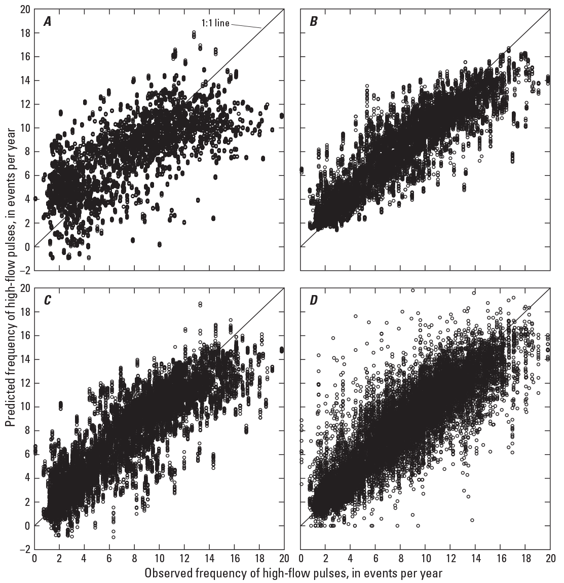
Observed versus predicted frequency of high-flow pulses. A, multiple linear regression; B, random forest, C, support vector regression; and D, cubist regression.
Generally, base flow and soil characteristics (such as soils in hydrologic group A) are the most common predictors of low-flow metrics (table 2). Spring and summer runoff and soil characteristics (silt and sand content percentages) are the top predictors of annual high-flow metrics (table 2).
Seasonal and Monthly Flow Metrics
In general, the RF approach results in the largest CPM values for the seasonal timing metrics and for monthly flow metrics (fig. 7). The seasonal and monthly flow metrics are more predictable during the wetter months in the United States (typically January through May) than the drier months (typically from June through September). Also, the high-flow metrics tend to be more predictable than low-flow metrics for all seasons. The flow metrics associated with higher flows are more predictable than those for low flows for every month. The predicted versus observed plots of the 20-percent nonexceedance flows in June (fig. 8) show that these approaches underpredict the larger values. Similar to the annual metrics, LR and SVR approaches predict negative flow values for small magnitude observed values.
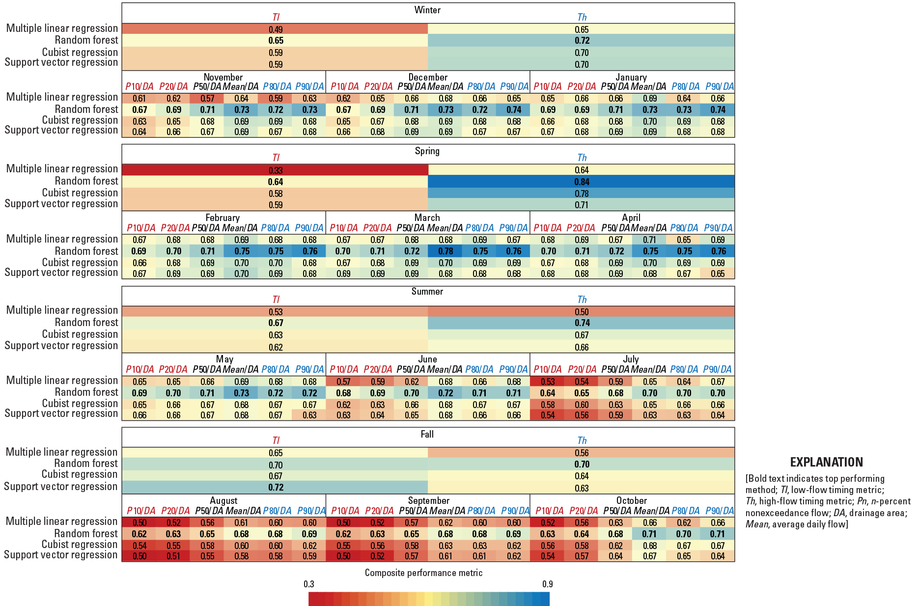
Performance metrics for the seasonal and monthly flow metrics.
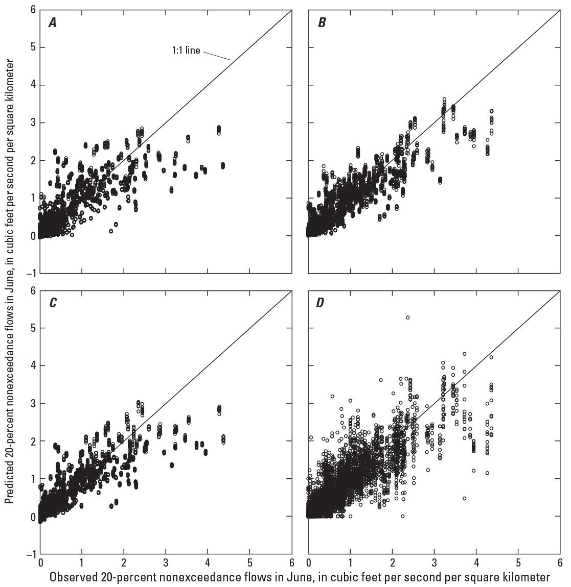
Observed versus predicted 20-percent nonexceedance flows in June. A, multiple linear regression; B, random forest; C, support vector regression; and D, cubist regression.
Runoff metrics are common significant predictors for most seasonal and monthly flow metrics (table 2). Base-flow measures also are significant predictors primarily for low and mean flow metrics. Precipitation, temperature, and soil metrics are less common predictors among these flow metrics compared to runoff or base flow.
Discussion on Performance of Approaches
This section compares the performance of machine learning approaches for some flow metrics to methods reported in the literature. Discussion of possible causes and solutions for poor performance by machine learning approaches also is described in this section. In addition, significant hydrological processes identified in the analysis are described. Lastly, limitations of the analysis are discussed.
Machine Learning Approaches
Generally, flow metrics describing median and high-flow events are more predictable than metrics for low-flow events regardless of the modeling approach. This result is consistent with Eng and others (2017) for RF and, in general, with the four approaches (except duration of high pulses) in Peñas and others (2018). Metrics based on the Julian day of high- and low-flow events to represent timing of these events are often unpredictable (Eng and others, 2017; Peñas and others, 2018). High- and low-flow timing metrics based on the frequency of occurrence, however, are predictable in this study and consistent with Eng and others (2019). For flood metrics, CR and SVR provided substantial gains in prediction accuracy compared to the conventional LR method. For extreme low-flow metrics, such as the 7-day, 10-year flow, Worland and others (2018) reported that CR outperforms the other methods evaluated including RF and SVR for a southeast region in the United States. For all other nonextreme flow metrics (except the timing of low-flow events in fall), RF outperforms other methods. Some of the predictive gains by RF compared to the other methods are marginal (for example, February median flow normalized by DA), whereas other gains are more substantial (for example, March mean flow normalized by DA) based on the CPM metric.
An advantage of using CR is that CR simplifies the tree into a set of rules and associated LRs that make CR much more intuitive for most users compared to the other machine learning approaches. CR is similar to region of influence approaches (for example, Burn, 1990; Eng and others, 2005), but instead of using a Euclidean metric to determine groups of similar observations in predictor-variable space, CR uses rules developed from splits in the tree (specifically, interactions among the predictor variables) to determine subspaces where those observations in each subspace would be fit with a LR. A weakness of LR is identification of these predictor variable interactions since they are required to be specified a priori in the initial formation of the model. This process is complicated when the pool of predictors is large. The large reductions in RMSE from LR to CR indicate that the relation among the predictand and predictors is not linear throughout the range of predictand values. CR is able to parse linear portions of the nonlinear relation to improve predictions.
RF is a widely applied method in hydrology, but RF performs poorly for flood metrics because of underprediction and overprediction at the minimum and maximum ranges of the flow metric values. This effect is a commonly reported problem with RF (for example, Zhang and Lu, 2012). Causes of this underprediction and overprediction could be due to the imbalance in the range of observation values of the training data (specifically, few observations at the extreme values relative to the median) (Chen and others, 2004; Zimmerman and others, 2018), the random selection of predictor variables used to determine splits, and the averaging of observations within the terminal nodes of each tree in the forest.
When few extreme observations are available, RF will tend to select a disproportionate number of observations not from the extremes when training tree models, and as a result, RF will underpredict or overpredict extreme values. Down sampling (specifically, reducing the number of observations, which results in about an equal number of observations throughout all ranges of values) nonextreme observations can be used to reduce the underpredictions or overpredictions at the extreme values (Chen and others, 2004). Down sampling, however, is not incorporated in the randomForest package in R (ver. 3.5.0; R Core Team 2018). For regression applications, binning would be required, such as using deciles and some number of observations pulled from each bin to achieve a dataset that has about equal representation throughout all values of the predictand.
For RF, the random selection of predictors at splits can result in trees that predict poorly if the predictand is highly dependent on a single predictor and the pool of predictors is large. For example, drainage area is typically the most dominant and significant predictor for flood metrics. If the frequency of using drainage area as a predictor is low for all trees in the forest, the averaged predictions will likely be poor. Weighting predictors or simply locking some to be chosen at the splits could reduce the formation of poorly predicting tree models.
Lastly, the averaging of observations in the terminal nodes of each tree in a forest could contribute to the underprediction and overprediction at extreme values of the observations and can be best demonstrated by the application to flood metrics. This averaging will push the predictions towards the median of observed values. Use of a regression function in the terminal nodes for the most extreme observed values could alleviate/reduce this underprediction and overprediction problem. CR and RF share this feature of using regression trees, but one primary difference between CR and RF is how the observations are treated in the nodes—CR uses LR, whereas RF uses an average value. CR does not have issues with underprediction and overprediction at the extreme ranges of the observations. The CPM accounts for percent bias throughout the range of observation values, so if predictions are systematically high or low for different portions of the predicted range (for example, for predictions of flood flows by RF), these systematic deviations can balance each other out.
Thus, the difference in performance of the machine learning approaches for the different flow metrics could be due to three factors—the imbalance in the range of observation values of the training data, the predictand being highly dependent on a single predictor (such as flood metrics), and the averaging of observations in the terminal nodes of RF.
Hydrological Processes
Climate is a primary variable that affects flooding through winter runoff and by intense and sustained orographic precipitation caused by atmospheric rivers (Ralph and others, 2006; Neiman and others, 2011). These atmospheric rivers are narrow corridors of highly intense water vapor transport in the lower atmosphere (Zhu and Newell, 1998; Ralph and others, 2004; Ralph and Dettinger, 2011). These corridors can occur during summer and winter, but the corridors that occur during winter are associated with stronger water vapor transport (Neiman and others, 2008). The seasonality of floods west of the Cascade Mountain Range (fig. 1) in the United States occur predominantly during winter (Mastin and others, 2016), and the partial dependency plot (fig. 9A) for December precipitation shows a linear increasing relation with floods.
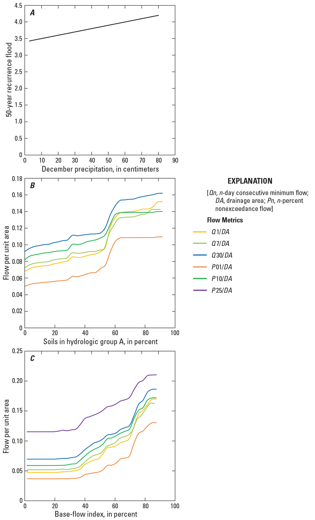
Partial dependency plots for models predicting three different flow metrics. A, logarithmic (base 10) transform of the 50-year recurrence flood and December precipitation; B, annual low flows and soils in hydrologic group A (high infiltration rates); and C, annual low flows and base-flow index.
In addition to climatic factors, hydrologic processes are affected by soil and lithologic characteristics. The effect of soil and lithology is quantified in the partial dependency plot (fig. 9B) for soils in hydrologic group A. This partial dependency plot clearly shows that runoff (flow per unit area) increases as the percentage of soils in hydrologic group A increases. This effect is expected because hydrologic group A is representative of well-drained soils with high permeability. These soil conditions promote rapid movement of water through the soil zone. This effect of well-drained soils also is supported by the partial dependency plot for the base-flow index (fig. 9C), which indicates high percentages of base flow in runoff that only will occur in areas conducive to subsurface flow. Base-flow variables are consistently shown to be significant for low-flow metrics (for example, Smakhtin, 2001). The soils in hydrologic group A and base-flow index variables are weakly correlated to one another (correlation coefficient, ρ, about equal to 0.3).
The application of the methods in this study assumes that the observations are independent of one another. For flood metrics, this assumption may be violated, and methods need to be developed to reweight observations when developing models, such as generalized least squares (GLS) regression (Stedinger and Tasker, 1985). However, development of equivalent GLS functionality for each machine learning approach is outside the scope of this study.
This study analysis assumed no significant trends in the flow metrics (in other words, no time-varying flow metrics). Nevertheless, the machine learning approaches in this study can be easily modified to produce time-varying predictions rather than static predictions using frameworks such as cross-section time series analysis (also referred to as “panel” analysis) or approaches developed by Miller and others (2018). Month-year specific flow metrics were predicted by Miller and others (2018) using a mixture of static and time-varying climate predictor variables, but a discussion of this approach is beyond the scope of this paper.
Lastly, the effect of redefining the regions of interest based on the results from this study are unknown. Inclusion or exclusion of additional basins as a result of extending or shrinking the study areas changes the robustness of the parameters of the models, and either increases or decreases the homogenization of the predictors and predictands. These changes could possibly change the results from this study. Analysis of these effects, however, also is outside the scope of this study.
Summary
This study provides a comprehensive evaluation of the streamflow regime based on three widely available machine learning approaches (support vector regression, random forest, and cubist regression) and for multiple linear regression to predict 106 natural streamflow metrics at ungaged locations. The results indicate that for flood metrics, predictions by cubist regression and support vector regressions have substantially less error than the other approaches. For all the remaining streamflow metrics, random forest models outperform the other methods. It should be noted that some of the predictive gains by random forest were modest, such as the gains for median and monthly flows.
Acknowledgments
The authors would like to thank Peter McCarthy, Adam Stonewall, and Alison Appling (U.S. Geological Survey) for their thoughtful comments, which improved the manuscript.
References Cited
Breiman, L., 2001, Random forests: Machine Learning, v. 45, no. 1, p. 5–32. [Also available at https://doi.org/10.1023/A:1010933404324.]
Burn, D.H., 1990, Evaluation of regional flood frequency analysis with a region of influence approach: Water Resources Research, v. 26, no. 10, p. 2257–2265. [Also available at https://doi.org/10.1029/WR026i010p02257.]
Carlisle, D.M., Falcone, J., Wolock, D.M., and Meador, M.R., 2010, Predicting the natural flow regime—Models for assessing hydrological alteration in streams: River Research and Applications, v. 26, no. 2, p. 118–136. [Also available at https://doi.org/10.1002/rra.1247.]
Carlisle, D.M., Grantham, T.E., Eng, K., and Wolock, D.M., 2017, Biological relevance of streamflow metrics—Regional and national perspectives: Freshwater Science, v. 36, no. 4, p. 927–940. [Also available at https://doi.org/10.1086/694913.]
Carlisle, D.M., Wolock, D.M., Howard, J.K., Grantham, T.E., Fesenmyer, K., and Wieczorek, M., 2016, Estimating natural monthly streamflows in California and the likelihood of anthropogenic modification: U.S. Geological Survey Open-File Report 2016–1189, 27 p. [Also available at https://doi.org/10.3133/ofr20161189.]
Chen, C., Liaw, A., and Breiman, L., 2004, Using random forest to learn imbalanced data—Technical report: Berkeley, University of California. [Also available at https://statistics.berkeley.edu/sites/default/files/tech-reports/666.pdf.]
Cooper, R.M., 2005, Estimation of peak discharges for rural, unregulated streams in western Oregon: U.S. Geological Survey Scientific Investigations Report 2005–5116, 134 p. [Also available at https://doi.org/10.3133/sir20055116.]
Dudley, R.W., 2015, Regression equations for monthly and annual mean and selected percentile streamflows for ungaged rivers in Maine (ver. 1.1, December 21, 2015): U.S. Geological Survey Scientific Investigations Report 2015–5151, 35 p. [Also available at https://doi.org/10.3133/sir20155151.]
Eng, K., 2022, Calculated streamflow metrics for machine learning regionalization across the conterminous United States, 1950 to 2018: U.S. Geological Survey data release, https://doi.org/10.5066/P9VQAZN7.
Eng, K., Carlisle, D.M., Grantham, T.E., Wolock, D.M., and Eng, R.L., 2019, Severity and extent of alterations to natural streamflow regimes based on hydrologic metrics in the conterminous United States, 1980–2014: U.S. Geological Survey Scientific Investigations Report 2019–5001, 25 p. [Also available at https://doi.org/10.3133/sir20195001.]
Eng, K., Grantham, T.E., Carlisle, D.M., and Wolock, D.M., 2017, Predictability and selection of hydrologic metrics in riverine ecohydrology: Freshwater Science, v. 36, no. 4, p. 915–926. [Also available at https://doi.org/10.1086/694912.]
Eng, K., Tasker, G.D., and Milly, P.C.D., 2005, An analysis of region-of-influence methods for flood regionalization in the Gulf-Atlantic Rolling Plains: Journal of the American Water Resources Association, v. 41, no. 1, p. 135–143. [Also available at https://doi.org/10.1111/j.1752-1688.2005.tb03723.x.]
England, J.F., Jr., Cohn, T.A., Faber, B.A., Stedinger, J.R., Thomas, W.O., Jr., Veilleux, A.G., Kiang, J.E., and Mason, R.R., Jr., 2019, Guidelines for determining flood flow frequency-bulletin 17C: U.S. Geological Survey Techniques and Methods 4–B5, 148 p. [Also available at https://doi.org/10.3133/tm4B5.]
Falcone, J.A., 2011, GAGES–II—Geospatial attributes of gages for evaluating streamflow: U.S. Geological Survey database, accessed September 28, 2020, at https://doi.org/10.3133/70046617.
Friedman, J.H., 2001, Greedy function approximation—A gradient boosting machine: Annals of Statistics, v. 29, no. 5, p. 1189–1232. [Also available at https://doi.org/10.1214/aos/1013203451.]
Greenwell, B., 2018, R package “pdp” (ver. 0.7.0): GitHub software, accessed September 28, 2020, at https://github.com/bgreenwell/pdp.
Gupta, H.V., Sorooshian, S., and Yapo, P.O., 1999, Status of automatic calibration for hydrologic models—Comparison with multilevel expert calibration: Journal of Hydrologic Engineering, v. 4, no. 2, p. 135–143. [Also available at https://doi.org/10.1061/(ASCE)1084-0699(1999)4:2(135).]
He, Z., Wen, X., Liu, H., and Du, J., 2014, A comparative study of artificial neural network, adaptive neuro fuzzy inference system and support vector machine for forecasting river flow in the semiarid mountain region: Journal of Hydrology, v. 509, p. 379–386. [Also available at https://doi.org/10.1016/j.jhydrol.2013.11.054.]
Jennings, M.E., Thomas, W.O., and Riggs, H.C., 1994, Nationwide summary of U.S. Geological Survey regional regression equations for estimating magnitude and frequency of floods for ungaged sites, 1993: U.S. Geological Survey Water-Resources Investigations Report 94–4002, 196 p. [Also available at https://doi.org/10.3133/wri944002.]
Jeong, D.-I., and Kim, Y.-O., 2005, Rainfall-runoff models using artificial neural networks for ensemble streamflow prediction: Hydrological Processes, v. 19, no. 19, p. 3819–3835. [Also available at https://doi.org/10.1002/hyp.5983.]
Kuhn, M., Weston, S., Keefer, C., Coulter, N., and Quinlan, R., and the Rulequest Research Pty Ltd, 2020a, Rule- and instance-based regression modeling—R package Cubist (ver. 0.2.3): GitHub software, accessed September 28, 2020, at https://topepo.github.io/Cubist.
Kuhn, M., Wing, J., Weston, S., Williams, A., Keefer, C., Engelhardt, A., Cooper, T., Mayer, Z., Kenkel, B., Benesty, M., Lescarbeau, R., Ziem, A., Scrucca, L., Tang, Y., Candan, C., and Hunt, T., 2020b, Classification and regression training—R package caret (ver. 6.0–86): GitHub software, accessed September 28, 2020, at https://github.com/topepo/caret/.
Liaw, A., and Wiener, M., 2018, Breiman and Cutler’s random forests for classification and regression—R package randomForest (ver. 4.6–14): University of California, Berkeley software, accessed September 28, 2020, at https://www.stat.berkeley.edu/~breiman/RandomForests/.
Lima, A.R., Cannon, A.J., and Hsieh, W.W., 2016, Forecasting daily streamflow using online sequential extreme learning machines: Journal of Hydrology, v. 537, p. 431–443. [Also available at https://doi.org/10.1016/j.jhydrol.2016.03.017.]
Lombard, P.J., 2004, August median streamflow on ungaged streams in eastern coastal Maine: U.S. Geological Survey Scientific Investigations Report 2004–5157, 22 p., accessed September 28, 2020, at https://pubs.usgs.gov/sir/2004/5157/.
Mastin, M.C., Konrad, C.P., Veilleux, A.G., and Tecca, A.E., 2016, Magnitude, frequency, and trends of floods at gaged and ungaged sites in Washington, based on data through water year 2014 (ver 1.2, November 2017): U.S. Geological Survey Scientific Investigations Report 2016–5118, 70 p. [Also available at https://doi.org/10.3133/sir20165118.]
Meyer, D., Dimitriadou, E., Hornik, K., Weingessel, A., Leisch, F., Chang, C.-C., and Lin, C.-C., 2019, Misc functions of the department of statistics, probability theory group (formerly: e1071), TU Wien: R package e1071 (ver. 1.7–3): R web page, accessed September 28, 2020, at https://cran.r-project.org/web/packages/e1071/index.html.
Miller, M.P., Carlisle, D.M., Wolock, D.M., and Wieczorek, M., 2018, A database of natural monthly streamflow estimates from 1950 to 2015 for the conterminous United States: Journal of the American Water Resources Association, v. 54, no. 6, p. 1258–1269. [Also available at https://doi.org/10.1111/1752-1688.12685.]
Mosavi, A., Ozturk, P., and Chau, K.-W., 2018, Flood prediction using machine learning models—Literature review: Water (Basel), v. 10, no. 11, 40 p. [Also available at https://doi.org/10.3390/w10111536.]
Nash, J.E., and Sutcliffe, J.V., 1970, River flow forecasting through conceptual models. Part 1—A discussion of principles: Journal of Hydrology, v. 10, no. 3, p. 282–290. [Also available at https://doi.org/10.1016/0022-1694(70)90255-6.]
Neiman, P.J., Ralph, F.M., Wick, G.A., Lundquist, J.D., and Dettinger, M.D., 2008, Meteorological characteristics and overland precipitation impacts of atmospheric rivers affecting the west coast of North America based on eight years of SSM/I satellite observations: Journal of Hydrometeorology, v. 9, no. 1, p. 22–47. [Also available at https://doi.org/10.1175/2007JHM855.1.]
Neiman, P.J., Schick, L.J., Ralph, F.M., Hughes, M., and Wick, G.A., 2011, Flooding in western Washington—The connection to atmospheric rivers: Journal of Hydrometeorology, v. 12, no. 6, p. 1337–1358. [Also available at https://doi.org/10.1175/2011JHM1358.1.]
Noori, R., Karbassi, A.R., Moghaddamnia, A., Han, D., Zokaei-Ashtiani, M.H., Farokhnia, A., and Gousheh, M.G., 2011, Assessment of input variables determination on the SVM model performance using PCA, Gamma test, and forward selection techniques for monthly stream flow prediction: Journal of Hydrology, v. 401, no. 3-4, p. 177–189. [Also available at https://doi.org/10.1016/j.jhydrol.2011.02.021.]
Peñas, F.J., Barquín, J., and Álvarez, C., 2018, A comparison of modeling techniques to predict hydrological indices in ungauged rivers: Limnetica, v. 37, no. 1, p. 145–158. [Also available at https://doi.org/10.23818/limn.37.12.]
R Core Team, 2018, R: A Language and Environment for Statistical Computing. R Foundation for Statistical Computing, Vienna accessed on 5/1/2018 at https://www.R-project.org.
Ralph, F.M., and Dettinger, M.D., 2011, Storms, floods and the science of atmospheric rivers: Eos (Washington, D.C.), v. 92, no. 32, p. 265–266. [Also available at https://doi.org/10.1029/2011EO320001.]
Ralph, F.M., Neiman, P.J., and Wick, G., 2004, Satellite and CALJET aircraft observations of atmospheric rivers over the eastern North Pacific Ocean during the winter of 1997/98: Monthly Weather Review, v. 132, no. 7, p. 1721–1745. [Also available at https://doi.org/10.1175/1520-0493(2004)132<1721:SACAOO>2.0.CO;2.]
Ries, K.G., III, Newson, J.K., Smith, M.J., Guthrie, J.D., Steeves, P.A., Haluska, T.L., Kolb, K.R., Thompson, R.F., Santoro, R.D., and Vraga, H.W., 2017, StreamStats, version 4: U.S. Geological Survey Fact Sheet 2017–3046, 4 p. [Also available at https://doi.org/10.3133/fs20173046.]
Ripley, B., Venables, B., Bates, D.M., Hornik, K., Gebhardt, A., and Firth, D., 2020, Support functions and datasets for Venables and Ripley’s MASS: R package MASS ver. 7.3–51.6, accessed September 28, 2020, at https://cran.r-project.org/web/packages/MASS/MASS.pdf.
Smakhtin, V.U., 2001, Low flow hydrology—A review: Journal of Hydrology, v. 240, no. 3–4, p. 147–186. [Also available at https://doi.org/10.1016/S0022-1694(00)00340-1.]
Smola, A.J., and Schölkopf, B., 2004, A tutorial on support vector regression: Statistics and Computing, v. 14, no. 3, p. 199–222. [Also available at https://doi.org/10.1023/B:STCO.0000035301.49549.88.]
Stedinger, J.R., and Tasker, G.D., 1985, Regional hydrologic analysis—1. ordinary, weighted, and generalized least squares compared: Water Resources Research, v. 21, no. 9, p. 1421–1432. [Also available at https://doi.org/10.1029/WR021i009p01421.]
Sun, A.Y., Wang, D., and Xu, X., 2014, Monthly streamflow forecasting using Gaussian process regression: Journal of Hydrology, v. 511, p. 72–81. [Also available at https://doi.org/10.1016/j.jhydrol.2014.01.023.]
Thomas, D.M., and Benson, M.A., 1970, Generalization of streamflow characteristics from drainage-basin characteristics: U.S. Geological Survey Water-Supply Paper 1975, 55 p. [Also available at https://doi.org/10.3133/wsp1975.]
Vapnik, V., 1995, The Nature of Statistical Learning Theory: New York, Springer. [Also available at https://doi.org/10.1007/978-1-4757-2440-0.]
Veilleux, A.G., Stedinger, J.R., and Lamontagne, J.R., 2011, Bayesian WLS/GLS regression for regional skewness analysis for regions with large cross-correlations among flood flows, paper 1303, in World Environmental and Water Resources Congress 2011—Bearing knowledge for sustainability, Palm Springs, Calif., May 22–26, 2011: American Society of Civil Engineers, p. 3103–3112.
Wilkowske, C.D., Kenney, T.A., and Wright, S.J., 2008, Methods for estimating monthly and annual streamflow statistics at ungaged sites in Utah: U.S. Geological Survey Scientific Investigations Report 2008–5230, 63 p. [Also available at https://pubs.usgs.gov/sir/2008/5230.]
Wolock, D.M., and McCabe, G.J., 1999, Explaining spatial variability in mean annual runoff in the conterminous United States: Climate Research, v. 11, p. 149–159. [Also available at https://doi.org/10.3354/cr011149.]https://doi.org/10.3354/cr011149
Wolock, D.M., Winter, T.C., and McMahon, G., 2004, Delineation and evaluation of hydrologic-landscape regions in the United States using geographic information system tools and multivariate statistical analyses: Environmental Management, v. 34, p. S71–S88. [Also available at https://doi.org/10.1007/s00267-003-5077-9.]
Wood, M.S., Fosness, R.L., Skinner, K.D., and Veilleux, A.G., 2016, Estimating peak-flow frequency statistics for selected gaged and ungaged sites in naturally flowing streams and rivers in Idaho (ver. 1.1, April 2017): U.S. Geological Survey Scientific Investigations Report 2016–5083, 56 p. [Also available at https://doi.org/10.3133/sir20165083.]
Worland, S.C., Farmer, W.H., and Kiang, J.E., 2018, Improving predictions of hydrological low-flow indices in ungaged basins using machine learning: Environmental Modelling & Software, v. 101, p. 169–182. [Also available at https://doi.org/10.1016/j.envsoft.2017.12.021.]
Zhang, G., and Lu, Y., 2012, Bias-corrected random forests in regression: Journal of Applied Statistics, v. 39, no. 1, p. 151–160. [Also available at https://doi.org/10.1080/02664763.2011.578621.]
Zhu, Y., and Newell, R.E., 1998, A proposed algorithm for moisture fluxes from atmospheric rivers: Monthly Weather Review, v. 126, no. 3, p. 725–735. [Also available at https://doi.org/10.1175/1520-0493(1998)126<0725:APAFMF>2.0.CO;2.]
Zimmerman, N., Presto, A.A., Kumar, S.P.N., Gu, J., Hauryliuk, A., Robinson, E.S., Robinson, A.L., and Subramanian, R., 2018, A machine learning calibration model using random forests to improve sensor performance for lower-cost air quality monitoring: Atmospheric Measurement Techniques, v. 11, no. 1, p. 291–313. [Also available at https://doi.org/10.5194/amt-11-291-2018.]
Appendix 1. 176 Basin Attributes and Corresponding Descriptions
Table 1.1.
176 basin attribute numbers, acronyms, and descriptions.| Basin attribute number | Basin attribute acronym | Description |
|---|---|---|
| 1 | DRAIN_SQKM | Watershed drainage area, in square kilometers. |
| 2 | PPTAVG_BASIN | Average annual precipitation for the watershed, in centimeters. |
| 3 | T_AVG_BASIN | Average annual air temperature for the watershed, in degrees Celsius. |
| 4 | RH_BASIN | Watershed average relative humidity, in percent. |
| 5 | FST32F_BASIN | Watershed average of mean day of the year of first freeze. |
| 6 | LST32F_BASIN | Watershed average of mean day of the year of last freeze. |
| 7 | WD_JAN_BASIN | Watershed average of number of days of measurable precipitation in January, in days. |
| 8 | WD_FEB_BASIN | Watershed average of number of days of measurable precipitation in February, in days. |
| 9 | WD_MAR_BASIN | Watershed average of number of days of measurable precipitation in March, in days. |
| 10 | WD_APR_BASIN | Watershed average of number of days of measurable precipitation in April, in days. |
| 11 | WD_MAY_BASIN | Watershed average of number of days of measurable precipitation in May, in days. |
| 12 | WD_JUN_BASIN | Watershed average of number of days of measurable precipitation in June, in days. |
| 13 | WD_JUL_BASIN | Watershed average of number of days of measurable precipitation in July, in days. |
| 14 | WD_AUG_BASIN | Watershed average of number of days of measurable precipitation in August, in days. |
| 15 | WD_SEP_BASIN | Watershed average of number of days of measurable precipitation in September, in days. |
| 16 | WD_OCT_BASIN | Watershed average of number of days of measurable precipitation in October, in days. |
| 17 | WD_NOV_BASIN | Watershed average of number of days of measurable precipitation in November, in days. |
| 18 | WD_DEC_BASIN | Watershed average of number of days of measurable precipitation in December, in days. |
| 19 | WD_BASIN | Watershed average of annual number of days of measurable precipitation, in days. |
| 20 | WDMAX_BASIN | Watershed average of monthly maximum number of days of measurable precipitation, in days. |
| 21 | WDMIN_BASIN | Watershed average of monthly minimum number of days of measurable precipitation, in days. |
| 22 | PET | Average annual potential evapotranspiration, in millimeters. |
| 23 | SNOW_PCT_PRECIP | Snow percent of total precipitation, in percent. |
| 24 | JAN_PPT_CM | Average January precipitation for the watershed, in centimeters. |
| 25 | FEB_PPT_CM | Average February precipitation for the watershed, in centimeters. |
| 26 | MAR_PPT_CM | Average March precipitation for the watershed, in centimeters. |
| 27 | APR_PPT_CM | Average April precipitation for the watershed, in centimeters. |
| 28 | MAY_PPT_CM | Average May precipitation for the watershed, in centimeters. |
| 29 | JUN_PPT_CM | Average June precipitation for the watershed, in centimeters. |
| 30 | JUL_PPT_CM | Average July precipitation for the watershed, in centimeters. |
| 31 | AUG_PPT_CM | Average August precipitation for the watershed, in centimeters. |
| 32 | SEP_PPT_CM | Average September precipitation for the watershed, in centimeters. |
| 33 | OCT_PPT_CM | Average October precipitation for the watershed, in centimeters. |
| 34 | NOV_PPT_CM | Average November precipitation for the watershed, in centimeters. |
| 35 | DEC_PPT_CM | Average December precipitation for the watershed, in centimeters. |
| 36 | JAN_TMP_DEGC | Average January air temperature for the watershed, in degrees Celsius. |
| 37 | FEB_TMP_DEGC | Average February air temperature for the watershed, in degrees Celsius. |
| 38 | MAR_TMP_DEGC | Average March air temperature for the watershed, in degrees Celsius. |
| 39 | APR_TMP_DEGC | Average April air temperature for the watershed, in degrees Celsius. |
| 40 | MAY_TMP_DEGC | Average May air temperature for the watershed, in degrees Celsius. |
| 41 | JUN_TMP_DEGC | Average June air temperature for the watershed, in degrees Celsius. |
| 42 | JUL_TMP_DEGC | Average July air temperature for the watershed, in degrees Celsius. |
| 43 | AUG_TMP_DEGC | Average August air temperature for the watershed, in degrees Celsius. |
| 44 | SEP_TMP_DEGC | Average September air temperature for the watershed, in degrees Celsius. |
| 45 | OCT_TMP_DEGC | Average October air temperature for the watershed, in degrees Celsius. |
| 46 | NOV_TMP_DEGC | Average November air temperature for the watershed, in degrees Celsius. |
| 47 | DEC_TMP_DEGC | Average December air temperature for the watershed, in degrees Celsius. |
| 48 | ET | Average annual evapotranspiration, in millimeters. |
| 49 | BEDROCK_PERM | Bedrock permeability class, dimensionless. |
| 50 | BFI_AVE | Base-flow index (BFI). The BFI is a ratio of base flow to total streamflow, expressed as a percentage and ranging from 0 to 100. Base flow is the sustained, slowly varying component of streamflow, usually attributed to groundwater discharge to a stream. |
| 51 | PERDUN | Dunne overland flow, also known as saturation overland flow, is generated in a basin when the water table "outcrops" on the land surface (due to the infiltration and redistribution of soil moisture within the basin), thereby producing temporary saturated areas. These saturated areas generate Dunne overland flow through exfiltration of shallow groundwater and by routing precipitation directly to the stream network. |
| 52 | PERHOR | Horton overland flow, also known as infiltration-excess overland flow, is generated in a basin when infiltration rates are exceeded by precipitation rates. |
| 53 | TOPWET | Topographic wetness index, ln(a/S); where “ln” is the natural log, “a” is the upslope area per unit contour length and “S” is the slope at that point. |
| 54 | CONTACT | Subsurface flow contact time index. The subsurface contact time index estimates the number of days that infiltrated water resides in the saturated subsurface zone of the basin before discharging into the stream. |
| 55 | RUNAVE | Estimated watershed annual runoff, in millimeters per year. |
| 56 | WB_JAN_MM | Estimated watershed January runoff, in millimeters per month. |
| 57 | WB_FEB_MM | Estimated watershed February runoff, in millimeters per month. |
| 58 | WB_MAR_MM | Estimated watershed March runoff, in millimeters per month. |
| 59 | WB_APR_MM | Estimated watershed April runoff, in millimeters per month. |
| 60 | WB_MAY_MM | Estimated watershed May runoff, in millimeters per month. |
| 61 | WB_JUN_MM | Estimated watershed June runoff, in millimeters per month. |
| 62 | WB_JUL_MM | Estimated watershed July runoff, in millimeters per month. |
| 63 | WB_AUG_MM | Estimated watershed August runoff, in millimeters per month. |
| 64 | WB_SEP_MM | Estimated watershed September runoff, in millimeters per month. |
| 65 | WB_OCT_MM | Estimated watershed October runoff, in millimeters per month. |
| 66 | WB_NOV_MM | Estimated watershed November runoff, in millimeters per month. |
| 67 | WB_DEC_MM | Estimated watershed December runoff, in millimeters per month. |
| 68 | WB_ANN_MM | Estimated watershed annual runoff, in millimeters per year. |
| 69 | DEPTH_WATTAB | Average value of depth to seasonally high water table, in feet. |
| 70 | HGA | Percentage of soils in hydrologic group A. Hydrologic group A soils have high infiltration rates. Soils are deep and well drained and, typically, have high sand and gravel content. |
| 71 | HGB | Percentage of soils in hydrologic group B. Hydrologic group B soils have moderate infiltration rates. Soils are moderately deep, moderately well drained, and moderately coarse in texture. |
| 72 | HGAD | Percentage of soils in hydrologic group A/D. Hydrologic group A/D soils have group A characteristics (high infiltration rates) when artificially drained and have group D characteristics (very slow infiltration rates) when not drained. |
| 73 | HGC | Percentage of soils in hydrologic group C. Hydrologic group C soils have slow soil infiltration rates. The soil profiles include layers impeding downward movement of water and, typically, have moderately fine or fine texture. |
| 74 | HGD | Percentage of soils in hydrologic group D. Hydrologic group D soils have very slow infiltration rates. Soils are clayey, have a high water table, or have a shallow impervious layer. |
| 75 | HGAC | Percentage of soils in hydrologic group A/C. Hydrologic group A/C soils have group A characteristics (high infiltration rates) when artificially drained and have group C characteristics (slow infiltration rates) when not drained. |
| 76 | HGBD | Percentage of soils in hydrologic group B/D. Hydrologic group B/D soils have group B characteristics (moderate infiltration rates) when artificially drained and have group D characteristics (very slow infiltration rates) when not drained. |
| 77 | HGCD | Percentage of soils in hydrologic group C/D. Hydrologic group C/D soils have group C characteristics (slow infiltration rates) when artificially drained and have group D characteristics (very slow infiltration rates) when not drained. |
| 78 | HGBC | Percentage of soils in hydrologic group B/C. Hydrologic group B/C soils have group B characteristics (moderate infiltration rates) when artificially drained and have group C characteristics (slow infiltration rates) when not drained. |
| 79 | AWCAVE | Average value for the range of available water capacity for the soil layer or horizon, in inches of water per inches of soil depth. |
| 80 | PERMAVE | Average permeability, in inches per hour. |
| 81 | BDAVE | Average value of bulk density, in grams per cubic centimeter. |
| 82 | OMAVE | Average value of organic matter content, in percent by weight. |
| 83 | WTDEPAVE | Average value of depth to seasonally high water table, in feet. |
| 84 | ROCKDEPAVE | Average value of total soil thickness examined, in inches. |
| 85 | NO4AVE | Average value of percent by weight of soil material less than 3 inches in size and passing a No. 4 sieve (5 millimeters). |
| 86 | NO200AVE | Average value of percent by weight of soil material less than 3 inches in size and passing a No. 200 sieve (.074 millimeters). |
| 87 | NO10AVE | Average value of percent by weight of soil material less than 3 inches in size and passing a No. 10 sieve (2 millimeters). |
| 88 | CLAYAVE | Average value of clay content, in percent. |
| 89 | SILTAVE | Average value of silt content, in percent. |
| 90 | SANDAVE | Average value of sand content, in percent. |
| 91 | KFACT_UP | Average K-factor value for the uppermost soil horizon in each soil component. K-factor is an erodibility factor which quantifies the susceptibility of soil particles to detachment and movement by water. The K-factor is used in the Universal Soil Loss Equation (USLE) to estimate soil loss by water. Higher values of K-factor indicate greater potential for erosion. |
| 92 | RFACT | Rainfall and Runoff factor (“R factor” of Universal Soil Loss Equation) |
| 93 | SLOPE_PCT_30M | Mean watershed slope, in percent. |
| 94 | HLR1 | Areal extent of Hydrologic Landscape Region 1 in watershed, in percent. |
| 95 | HLR2 | Areal extent of Hydrologic Landscape Region 2 in watershed, in percent. |
| 96 | HLR3 | Areal extent of Hydrologic Landscape Region 3 in watershed, in percent. |
| 97 | HLR4 | Areal extent of Hydrologic Landscape Region 4 in watershed, in percent. |
| 98 | HLR5 | Areal extent of Hydrologic Landscape Region 5 in watershed, in percent. |
| 99 | HLR6 | Areal extent of Hydrologic Landscape Region 6 in watershed, in percent. |
| 100 | HLR7 | Areal extent of Hydrologic Landscape Region 7 in watershed, in percent. |
| 101 | HLR8 | Areal extent of Hydrologic Landscape Region 8 in watershed, in percent. |
| 102 | HLR9 | Areal extent of Hydrologic Landscape Region 9 in watershed, in percent. |
| 103 | HLR10 | Areal extent of Hydrologic Landscape Region 10 in watershed, in percent. |
| 104 | HLR11 | Areal extent of Hydrologic Landscape Region 11 in watershed, in percent. |
| 105 | HLR12 | Areal extent of Hydrologic Landscape Region 12 in watershed, in percent. |
| 106 | HLR13 | Areal extent of Hydrologic Landscape Region 13 in watershed, in percent. |
| 107 | HLR14 | Areal extent of Hydrologic Landscape Region 14 in watershed, in percent. |
| 108 | HLR15 | Areal extent of Hydrologic Landscape Region 15 in watershed, in percent. |
| 109 | HLR16 | Areal extent of Hydrologic Landscape Region 16 in watershed, in percent. |
| 110 | HLR17 | Areal extent of Hydrologic Landscape Region 17 in watershed, in percent. |
| 111 | HLR18 | Areal extent of Hydrologic Landscape Region 18 in watershed, in percent. |
| 112 | HLR19 | Areal extent of Hydrologic Landscape Region 19 in watershed, in percent. |
| 113 | HLR20 | Areal extent of Hydrologic Landscape Region 20 in watershed, in percent. |
| 114 | gneiss | A metamorphic rock characterized by layers or aligned streaks of mineral grains. Gneiss can be formed from sedimentary, volcanic, or plutonic rocks by intense metamorphism and deformation (Reed and Bush, 2005). |
| 115 | granitic | Light-colored plutonic rocks composed chiefly of quartz and feldspar and small amounts of mica, hornblende, and other minerals (Reed and Bush, 2005). |
| 116 | ultramafic | Dark-colored plutonic or volcanic rocks composed chiefly of feldspar and dark minerals rich in iron and magnesium, such as hornblende, pyroxene, and olivine, and containing little or no quartz (Reed and Bush, 2005). |
| 117 | Quarternary | Rock from the last period of the Cenozoic Era. It began about 1.8 million years ago and extends to the present. (Reed and Bush, 2005). |
| 118 | sedimentary | Rocks composed of material derived from weathering or disintegration of older rocks that was transported and deposited by water, air, or ice, or of material that accumulates by other natural agents, such as chemical precipitation from solution or secretion by organisms (Reed and Bush, 2005). |
| 119 | volcanic | Finely crystalline or glassy igneous rocks that form by volcanic action at or near the surface (Reed and Bush, 2005). |
| 120 | water | Water (Reed and Bush, 2005). |
| 121 | Anorthosite | A plutonic rock composed almost entirely of calcium-rich feldspar (Reed and Bush, 2005). |
| 122 | intermediate | Medium- to dark-gray plutonic or volcanic rocks composed of roughly equal amounts of quartz, feldspar, mica, and hornblende. (Reed and Bush, 2005). |
| 123 | SGEO1 | si - Sea islands, in percent (Hunt, 1979). |
| 124 | SGEO2 | cr - Coral, in percent (Hunt, 1979). |
| 125 | SGEO3 | bm - Backshore deposits, in percent (Hunt, 1979). |
| 126 | SGEO4 | pW - Pre-Wisconsinan drift, in percent (Hunt, 1979). |
| 127 | SGEO5 | tg - Till, or ground moraine, in percent (Hunt, 1979). |
| 128 | SGEO6 | ts - Ice-laid deposits, like tg but mostly sand and silt, in percent (Hunt, 1979). |
| 129 | SGEO7 | ts/K,T - Thin ice-laid deposits, like ts but thin and discontinuous. Extensive exposure of underlying Cretaceous- and Tertiary-age formations, in percent (Hunt, 1979). |
| 130 | SGEO8 | mg - Deposits of mountain glaciers, in percent (Hunt, 1979). |
| 131 | SGEO9 | w - Gravel, sand and clay deposited by glacial streams adjacent to or downstream from temporary ice fronts, in percent (Hunt, 1979). |
| 132 | SGEO10 | al - Floodplain and alluvium gravel terraces, in percent (Hunt, 1979). |
| 133 | SGEO11 | fg - Fan gravels, in percent (Hunt, 1979). |
| 134 | SGEO12 | fs - Fan sands, in percent (Hunt, 1979). |
| 135 | SGEO13 | osg - Pliocene-age and older stream deposits on the Great Plains, in percent (Hunt, 1979). |
| 136 | SGEO14 | l - Lake deposits, in percent (Hunt, 1979). |
| 137 | SGEO15 | s - Sand sheets, mostly with dunes or sand mounds at surface, in percent (Hunt, 1979). |
| 138 | SGEO16 | s/osg - Sand sheets on sandy and gravelly Ogallala Formation in southern Great Plains, in percent (Hunt, 1979). |
| 139 | SGEO17 | wl - Wisconsinan loess, in percent (Hunt, 1979). |
| 140 | SGEO18 | es - Deeply weathered loess, in percent (Hunt, 1979). |
| 141 | SGEO19 | b - Basalt, in percent (Hunt, 1979). |
| 142 | SGEO20 | br - Bedrock, in percent (Hunt, 1979). |
| 143 | SGEO21 | rsh - Micaceous residuum without much quartz; clay mostly kaolinite, in percent (Hunt, 1979). |
| 144 | SGEO22 | rgr - Residuum with abundant quartz; much less mica than rsh, but equal to clay, in percent (Hunt, 1979). |
| 145 | SGEO23 | rga - Clay residuum with little mica or quartz; mostly massive kaolinitic clay, in percent (Hunt, 1979). |
| 146 | SGEO24 | rls - Red clay, massive clay that is generally kaolinitic, in percent (Hunt, 1979). |
| 147 | SGEO25 | rlc - Cherty red clay; similar to rls, but with chert from the parent rock, in percent (Hunt, 1979). |
| 148 | SGEO26 | rtr - Residuum on Triassic-age formations; depths less than most other saprolite, reddish color, largely inherited from parent rock, in percent (Hunt, 1979). |
| 149 | SGEO27 | rs - Sandy residuum, derived by intensive weathering of sandstone formations. Sand locally is in dunes, in percent (Hunt, 1979). |
| 150 | SGEO28 | rc - Clay residuum that swells when wet; developed by weathering of poorly consolidated shale, containing the clay mineral montmorillonite, generally less than 10 feet, in percent (Hunt, 1979). |
| 151 | SGEO29 | rl - Loam; texture variable, ranging from sand to clay, mostly non-swelling clay mineral, kaolinite; otherwise similar to rc, in percent (Hunt, 1979). |
| 152 | SGEO30 | rg - Intensively weathered upper Tertiary- and Quaternary-age gravels; thickness generally less than 30 feet, distribution not completely known, in percent (Hunt, 1979). |
| 153 | SGEO31 | rph - Phosphatic clay; poorly sorted clay and phosphate pebbles or nodules in sandy matrix. Thickness 10 to 50 feet, commonly overlain by loose sand. Major source of phosphate fertilizer, in percent (Hunt, 1979). |
| 154 | SGEO32 | rsi - Sandy or silty residuum; probably includes loess. Depth generally less than 10 feet, in percent (Hunt, 1979). |
| 155 | SGEO33 | ls - Silt on limestone; probably includes considerable loess; extensive bare rock, in percent (Hunt, 1979). |
| 156 | SGEO34 | ss - Sandy ground; mostly on poorly consolidated sandstone formations, in percent (Hunt, 1979). |
| 157 | SGEO35 | sh - Shaley or sandy ground; on mixed sandstone and shale formations; where shaley, contains considerable swelling clay, in percent (Hunt, 1979). |
| 158 | SGEO36 | gyp - Sandy gypsiferous ground; many sinks, local dunes; vegetation scanty or lacking where there is much gypsum or other salt, in percent (Hunt, 1979). |
| 159 | SGEO37 | c - Clayey ground on weathered Permian- and/or Triassic-age red beds, in percent (Hunt, 1979). |
| 160 | SGEO38 | m - Marshes, swamps, peat deposits; only locally thicker than 12 feet, in percent (Hunt, 1979). |
| 161 | SGEO39 | gp - Sandy coastal ground with organic layer over a shallow water table, groundwater podsols, in percent (Hunt, 1979). |
| 162 | SGEO40 | co/ss,sh - Sandy and stony colluvium derived mostly from sandstone and shale, in percent (Hunt, 1979). |
| 163 | SGEO41 | co/ls - Stony colluvium on limestone; considerable admixed silt, possibly of loess origin, in percent (Hunt, 1979). |
| 164 | SGEO42 | co/m - Stony colluvium on metamorphic rocks; less silt and clay than in co/ls, in percent (Hunt, 1979). |
| 165 | SGEO43 | co/v - Colluvium on volcanic rocks, in percent (Hunt, 1979). |
| 166 | SGEO44 | co/gr - Bouldery and sandy colluvium on granitic rocks, in percent (Hunt, 1979). |
| 167 | SGEO45 | co/c - Clayey and loamy colluvium; on poorly consolidated rocks on lee sides of Pacific Coast Ranges, in percent (Hunt, 1979). |
| 168 | cao20mar14 | Rock calcium oxide concentration, in percent. |
| 169 | fe20mar141 | Rock iron oxide concentration, in percent. |
| 170 | k20mar141 | Rock potassium oxide concentration, in percent. |
| 171 | mgo20mar141 | Rock magnesium oxide concentration, in percent. |
| 172 | p20mar141 | Rock phosphorus concentration, in percent. |
| 173 | perm20mar14 | Rock hydraulic conductivity, in 10-6 meters per second. |
| 174 | s20mar141 | Rock sulfur concentration, in percent. |
| 175 | si20mar141 | Rock silicon oxide concentration, in percent. |
| 176 | ucs20mar141 | Rock uniaxial compressive strength, in megapascals. |
References Cited
Reed, J.C., Jr., and Bush, C.A., 2005, Generalized geologic map of the United States, Puerto Rico, and the U.S. Virgin Islands: U.S. Geological Survey, National Atlas of the United States of America. [Also available at https://pubs.usgs.gov/atlas/geologic/.]
For more information about this publication, contact:
Program Coordinator, USGS Water Availability and Use Science Program
12201 Sunrise Valley Drive
Reston, VA 20192
703–648–5953
For additional information, visit: https://www.usgs.gov/programs/water-availability-and-use-science-program
Publishing support provided by the
Reston and Rolla Publishing Service Centers
Disclaimers
Any use of trade, firm, or product names is for descriptive purposes only and does not imply endorsement by the U.S. Government.
Although this information product, for the most part, is in the public domain, it also may contain copyrighted materials as noted in the text. Permission to reproduce copyrighted items must be secured from the copyright owner.
Suggested Citation
Eng, K., and Wolock, D.M., 2022, Evaluation of machine learning approaches for predicting streamflow metrics across the conterminous United States: U.S. Geological Survey Scientific Investigations Report 2022–5058, 27 p., https://doi.org/10.3133/sir20225058.
ISSN: 2328-0328 (online)
Study Area
| Publication type | Report |
|---|---|
| Publication Subtype | USGS Numbered Series |
| Title | Evaluation of machine learning approaches for predicting streamflow metrics across the conterminous United States |
| Series title | Scientific Investigations Report |
| Series number | 2022-5058 |
| DOI | 10.3133/sir20225058 |
| Publication Date | August 31, 2022 |
| Year Published | 2022 |
| Language | English |
| Publisher | U.S. Geological Survey |
| Publisher location | Reston, VA |
| Contributing office(s) | WMA - Integrated Modeling and Prediction Division |
| Description | Report: iv, 27 p.; Data Release |
| Country | United States |
| Online Only (Y/N) | Y |
| Additional Online Files (Y/N) | N |