

Analysis of Groundwater and Surface Water in Areas of Isoxaflutole Application, Tuscola and Kalamazoo Counties, Michigan
Links
- Document: Report (17.3 MB pdf) , HTML , XML
- NGMDB Index Page: National Geologic Map Database Index Page (html)
- Download citation as: RIS | Dublin Core
Acknowledgments
The authors gratefully acknowledge the assistance of landowners in Tuscola and Kalamazoo Counties who permitted access to their property for equipment installation and sample collection. The authors also gratefully acknowledge the assistance of Bob Pigg, Michigan Department of Agriculture and Rural Development, and Tianbo Xu, Bayer CropScience, for help with site selection, sampling design, and well installations and closures.
Abstract
The herbicide 5-cyclopropyl-4-(2-methylsulfonyl-4-trifluoromethylbenzoyl) isoxazole, also known as isoxaflutole (IXF), was conditionally approved for use on corn in Michigan in 2015. The fate of IXF and its degradates in different environmental settings and the processes by which these compounds move to groundwater or to surface-water bodies have been previously studied, but little information about possible persistence and buildup of this herbicide and its degradates in Michigan’s groundwater and surface water is available. Therefore, from 2015 to 2020, the U.S. Geological Survey, in cooperation with the Michigan Department of Agriculture and Rural Development, studied IXF and two of its degradates in two locations where IXF was applied.
IXF and its degradates were rarely detected in shallow groundwater downgradient from IXF applications. In contrast, one or more of the three target IXF compounds were detected in 40 percent of surface-water samples. The degradates 1-(2-methylsulfonyl-4-trifluoromethylphenyl)-2-cyano-3-cyclopropyl propan-1-dione), also known as diketonitrile isoxaflutole (DKN), and 2-methylsulfonyl-4-(trifluoromethyl) benzoic acid (BAA), the benzoic acid analogue of IXF, were detected more frequently than the parent compound. At surface-water sites, DKN and BAA reached maximum concentrations within about the first 5 weeks after IXF application after rainfall-runoff events. Concentrations subsequent to post-application maxima decreased through time approximately following first-order, exponential loss kinetics. Carryover of DKN and BAA, from an application year to the following spring, occurred at several surface-water sites, and springtime concentrations were typically 1–5 percent of maximum, post-application concentrations. Virtually no detections were recorded later in the growing season during non-application years. Results indicate rapid loss of IXF and very few detections of the parent compound from the study areas. The degradates DKN and BAA were more frequently detected in surface runoff up to about 1 year after IXF application, but no evidence of longer-term accumulation was found.
Introduction
Michigan has a diverse agricultural industry with over 200 commodities, including corn, soybeans, vegetables, fruits, and sugar beets (Michigan Farm Bureau, 2016). For optimum plant health and increased yields, pesticides and herbicides are often used to control weeds, pests, or plant diseases. In times of low rainfall, irrigation is often necessary to relieve, balance, or eliminate moisture stress. The frequency and amount of agricultural chemical and irrigation water use can vary from year to year depending on several factors, including crop type, resource availability, and local management decisions. In addition, field conditions, weather, rotation schedules, and soil moisture may also affect their application. Although these practices enable agricultural areas to be more productive, under some conditions excess chemicals may be washed from the application areas through tile drains, run off into nearby lakes or rivers, or absorbed beneath the root zone to the water table. This water may then be unsafe for use by humans or for use on other crops if the chemicals persist in the water supply.
The Michigan Department of Agriculture and Rural Development (MDARD) has responsibility for safeguarding the public’s food supply, controlling plant pests and diseases that threaten the food and agriculture system, and preserving the environment by which the farming community makes their living and feeds consumers. Accordingly, MDARD is interested in investigating the potential effects of a new herbicide, 5-cyclopropyl-4-(2-methylsulfonyl-4-trifluoromethylbenzoyl) isoxazole, also known as isoxaflutole (IXF), conditionally approved in 2015 for use on corn in Michigan. Because Michigan has different soil and climate conditions than other areas where this herbicide has been used, little information about possible persistence and buildup of this herbicide and its metabolites in groundwater and surface water has yet been gathered. Michigan has irrigated fields in areas of sandy soils and agricultural fields in areas of clay soils, leading to concerns about IXF movement to groundwater and runoff to adjacent surface-water bodies. In addition, because of the wide array of irrigated crops in Michigan, concerns that persistence and buildup of IXF in groundwater or surface water could negatively impact other irrigated crops in areas with upgradient application of IXF continues. From 2015 to 2020, the U.S. Geological Survey (USGS), in cooperation with MDARD, investigated IXF and its degradates in shallow groundwater and edge-of-field surface runoff. Water samples were collected before and after IXF application, and upgradient and downgradient from fields where IXF was applied.
Purpose and Scope
The purpose of this report is to summarize the water quality and hydrologic data collected at two IXF application areas during 2015–20. Data collection included groundwater samples, pond samples, and groundwater levels at the groundwater study area and surface-water and runoff samples, tile, and precipitation at the surface-water study area. Data analysis included the investigation of sample results and potential trends in concentrations over the study. These analyses were primarily for IXF and its two degradates, 1-(2-methylsulfonyl-4-trifluoromethylphenyl)-2-cyano-3-cyclopropyl propan-1-dione), also known as diketonitrile isoxaflutole (DKN), and 2-methylsulfonyl-4-(trifluoromethyl) benzoic acid, the benzoic acid analogue of isoxaflutole (BAA). Characterizing IXF and its degradates, assessing the persistence of IXF and its degradates in groundwater and surface water near or downstream from the application areas, and summarizing and analyzing data for 223 additional pesticides and pesticide degradates at the study sites are the objectives of this report.
Description of Isoxaflutole Characteristics
Isoxaflutole, Chemical Abstracts Service Registry Number (CASRN) 141112–29–0, Rhone-Poulenc Ag Company [RPA] 201772, is distributed by Bayer CropScience (Chesterfield, Missouri) and was registered for use in 24 States in 2011 (U.S. Environmental Protection Agency, 2011). IXF was initially produced by the Rhone-Poulenc Ag Company, which became Aventis CropScience which was then acquired by Bayer CropScience in 2001 (Sourcewatch, 2016); Rhone-Poulenc Ag Company (RPA) numbers are included here to facilitate comparison with other literature. IXF is a member of the benzoyl isoxazole family and is marketed as a low-application-rate pre-emergent herbicide for control of broadleaf weeds and some grasses in field corn (Pallett and others, 2001). The maximum seasonal application rate is 0.14 pound (lb) active ingredient/per acre, but recommended rates range down to 0.047 lb active ingredient/per acre. Use rates vary by soil texture, organic matter content, and use pattern. Generally, one application is made during a season. This herbicide acts by disrupting pigment biosynthesis in plants so emerging weeds are bleached as the herbicide is taken up by the root system. Under typical field conditions, IXF degrades quickly to the biologically active DKN (CASRN 143701–75–1; RPA 202248) through an opening of the isoxazole ring, followed by subsequent hydrolization to the inactive form BAA. From 2000 to 2008, an estimated annual 300,000 lb of IXF was applied in the United States on an estimated average of 5 percent of all U.S. corn (U.S. Environmental Protection Agency, 2011). In 2014 and 2015, estimated usage of IXF increased to over 550,000 lb in the United States (U.S. Geological Survey, 2015). In 2016 and 2017, usage increased to almost 600,000 lb in the United States.
IXF was conditionally registered by the U.S. Environmental Protection Agency (EPA, 1998) in 1998 for use on corn in 15 States and part of Texas. At that time, conditional, time-limited, and geographically limited registrations were permitted with restrictions for use based on field characteristics and method and amounts of application. Principal concerns of the EPA were that IXF degradates have properties and characteristics similar to other compounds detected in groundwater and surface water, and indications from short-term (1–2 years) study results suggest that IXF and its primary metabolite DKN had the potential to persist and accumulate potentially affecting growth and yield of non-target plants. Possible adverse effects on nearby non-target plants or aquatic organisms from spray drift or runoff also was a concern. Some studies (W.P. Eckel, EPA, written commun, 2001) showed the potential for IXF to contaminate shallow groundwater (less than about 10 feet to the water table) in areas with soils that are not normally considered vulnerable and that the preferential flow paths are a factor in groundwater contamination, especially in soils that are otherwise resistant to this problem. Under the conditional registration, additional studies were required to investigate the potential for groundwater contamination and to monitor surface-water quality.
Bayer CropScience (2004) did many studies to assess the fate of IXF residues and its degradates in different environmental settings and the processes by which these compounds move to groundwater or to surface-water bodies. Prospective groundwater studies from 1999 to 2001 in Nebraska, Iowa, and Indiana indicated that IXF and its biologically active degradate DKN generally degrade in the surface and subsoil before movement to groundwater when used according to label instructions. Occasional preferential flow in fields with shallow water tables and standing water was observed; however, residues continued to degrade and remained in the upper 5 feet of the water table (Bayer CropScience, 2004). Another study of residential wells in Nebraska was done after detection of DKN in monitoring wells near a reservoir. Samples were collected from 2000 until 2004. DKN was detected several times with a maximum concentration of 0.2 µg/L (micrograms per liter) in 2003 after a rain event soon after IXF application. This reservoir was constructed to recharge groundwater into the surficial aquifer, which helps to explain the DKN detections. Sampling of residential wells in the area in 2004 indicated no detections of DKN.
Runoff studies in Iowa and Illinois indicated that residue detections were correlated with rainfall events and that runoff concentration amounts varied according to the magnitude and intensity of storm events and the amount of crop coverage on the soil surface. Herbicide losses were highest after the first major rainfall event and declined significantly with subsequent events (Bayer CropScience, 2004). This effect of highest herbicide concentrations in runoff after the first rainfall event after application in the spring has been observed frequently and has been termed “spring flush” by other researchers (Goolsby and others, 1991a; Thurman and others, 1991; Battaglin and others, 2003; and Scribner and others, 2005). Scribner and others (2006) collected surface-water samples near the mouths of major rivers in Iowa to see if various herbicides and herbicide degradation products could be detected there. Of the 75 samples collected to measure IXF and its degradates, there were 4 detections of IXF, 56 detections of DKN, and 43 detections of BAA. Detections of IXF were from samples collected during the post-planting (May–June) season, whereas DKN and BAA were in samples from all sampling periods (pre-planting [March–April], post-planting, and late summer [July–September]). Maximum concentrations were observed in samples collected during the post-planting season and equaled 0.077 µg/L for IXF, 0.552 µg/L for DKN, and 0.166 µg/L for BAA. Concentrations of these compounds declined in samples collected in late summer.
Studies of the movement of IXF and degradates through tile drain systems were done by Bayer CropScience at seven locations in Ohio, Iowa, and Indiana in 1999 and 2000 (Bayer CropScience, 2004). Sample collection was carried out at the tile drain outlet, the receiving ditch, and a downstream point where flow was sufficient to act as an irrigation source. These studies demonstrated that highest concentrations generally were observed in early summer samples after sizeable rainfall amounts in the first few weeks after IXF application. Maximum concentrations of 5.6 µg/L for IXF, 62.6 µg/L for DKN, and 11.1 µg/L for BAA were observed in tile drains at an Indiana site in early summer. These concentrations fluctuated in relation to rain events and generally decreased to <1 µg/L for each compound in late summer and fall samples. Maximum concentrations of 0.08 µg/L for IXF, 14.1 µg/L for DKN, and 1.5 µg/L for BAA were observed in ditch samples at Iowa and Ohio sites in early summer. Concentrations in stream samples were generally <0.03 µg/L for IXF, <1 µg/L for DKN, and <0.5 µg/L for BAA in early summer samples. Higher concentrations above the reporting levels of IXF and its degradates were not observed in tile, ditch, or stream samples collected in August after the typical summer dry period at these sites (Bayer CropScience, 2004).
Except for one study in Ohio, IXF was applied once to each study area. One area experienced drought conditions after application in 1999, and no samples could be collected after the first rainfall until winter. IXF was reapplied in 2000, and samples were collected throughout the year after application. Concentrations in these samples were generally less than detection in late season samples. Due to this being the only study having more than one application and the varied soil conditions in Michigan, MDARD needed more information about the potential behavior and possible persistence of IXF or its degradates at or near application areas. Therefore, this study investigated IXF and degradate concentrations under different field conditions with multiple applications over a 5–year study.
Methods of Investigation
The methods of investigation for this study encompass site selection, study design and sample collection, field methods, and data preparation and analysis. Site selection includes a description of characteristics important for each study area. Study design and sample collection includes a description of the timing and frequency of environmental sample collection at each site and a description of the quality control samples collected during the study. All analytical results are stored in the USGS National Water Information System database (U.S. Geological Survey, 2022). Field methods include a description of the equipment used in this study and the collection, preparation, and handling of the samples from each site. Data preparation and analysis describes the data processing and statistical tests used to analyze sample results and characterize water quality at each site.
Study Area Selection
Selection of suitable areas for monitoring groundwater and surface water was based on several criteria, including 2013 crop data, soil properties (including drainage, texture, slope, and hydrologic group), distance to nearest waterbody, and depth to water. Area selection also was dependent on (1) soil types, soil properties, and other characteristics meeting herbicide usage requirements; (2) IXF not having been applied to the field in the past; (3) landowner participation in the study for 5 years; and (4) landowner agreement to grow corn and apply IXF in years 1 (2015), 3 (2017), and 5 (2019) of the study.
The groundwater study area needed excess water to infiltrate into the water table, so IXF or its degradates would be detected when groundwater samples were taken, if present. Further considerations at the groundwater site included the depth to water. Groundwater at shallower depths beneath fields would be more likely to be impacted by IXF or its degradates than water at deeper depths beneath fields with similar soil types and recharge conditions. Southwest Michigan was targeted for groundwater monitoring due to the presence of coarser soils and few tile drains, which met these requirements.
The surface-water study area needed excess water from the field to run off directly into an adjacent drain or stream or be intercepted by tiles in the field, which would then discharge into an adjacent drain or stream. Additionally, a pond was desirable to determine whether any evidence for the persistence or buildup of IXF or its metabolites over time could be documented. The distance to nearby surface-water features was another consideration when determining a potential surface-water site. Because monitoring at the surface-water site was intended to evaluate whether IXF was entering and persisting in a drain or stream, surface-water features needed to be adjacent to the selected field. The eastern side of Michigan was targeted for surface-water monitoring due to the prevalence of tile drained fields, which met these requirements.
Groundwater Study Area
The area selected for groundwater monitoring is in Texas Township in the southwestern part of Kalamazoo County in the southwestern Lower Peninsula of Michigan (fig. 1). Existing glacial wells in this area range in depth from 112 to 154 feet and have static water levels (at the time of well installation) ranging from 18 to 30 feet below land surface (Michigan Department of Environment, Great Lakes, and Energy, 2015). Rheaume (1990) reports that glacial deposits in this area generally range from 300 to 350 feet in thickness. The study area is in the Galesburg-Vicksburg outwash plain, which consists of medium- to very-coarse sand and gravel (Monaghan and others, 1983). This outwash area formed after the retreat and melting of the ice lobes that covered the county primarily during the Wisconsin glaciation about 15,000 to 17,000 years ago (Passero, 1978). Glacial deposits in this area overlie the Coldwater Shale bedrock unit of Mississippian age. This bedrock unit comprises shale that contains limestone and clayey limestone in some areas (Rheaume, 1990).
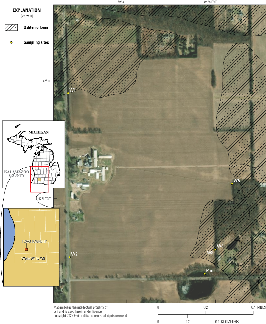
Groundwater study area and sampling sites, Kalamazoo County, Michigan.
Aquifers in the glacial deposits are the source of water for most of the county, whereas the shale unit underneath is rarely a source for water supply. Rheaume (1990) reported that groundwater moves from topographically high areas to discharge into ponds, streams, marshes, and other lowland areas. Annual cycles of higher groundwater levels in spring, and lower levels in fall, were apparent. Groundwater flows generally from west to east in the Kalamazoo County study field, and local flow moves toward a pond in the southeastern corner of the study area. Open lands, woodlands, and cultivated cropland are the primary land use categories in the county with corn, soybeans, and alfalfa being the primary crops planted in 2013.
The 240-acre Kalamazoo County field consists primarily of Kalamazoo Loam soils, but small areas in the north and east consist of Oshtemo Loam and areas in the south consist of Houghton Loam (Natural Resources Conservation Service, 2015). Kalamazoo Loam consists of loam, clay loam, loamy fine sand, and fine sand that are generally deep, well-drained soils formed in loess-influenced loamy outwash overlying sand, loamy sand, or sand and gravel outwash on outwash plains (U.S. Department of Agriculture-Natural Resources Conservation Service, 2015). Slopes range from 0 to 12 percent. These soils have a negligible to medium potential for surface runoff depending on the slope gradients. The Oshtemo Loam consists of sandy loam, loamy fine sand, and fine sand that are deep, well-drained soils formed in stratified loamy and sandy deposits on outwash plains. Slopes range from 1 to 12 percent. These soils have a runoff potential ranging from negligible to medium. The Oshtemo soil type has use restrictions preventing the application of IXF when the water table is less than 25 feet below the land surface (fig. 1). The Houghton Loam consists of deep, very poorly drained soils formed in herbaceous organic materials as depressions on lake or outwash plains. Slopes can range from 0 to 2 percent. These soils in a pond area at the site have a very slow potential for surface runoff. The cropping rotation at the site consisted of corn during years 1, 2, 3, and 5 and soybeans during year 4 of the monitoring period (calendar years 2015–19), and IXF applied only to the Kalamazoo Loam soils during the study.
Five wells were installed in April 2015 consisting of 2-inch polyvinyl chloride (PVC) casings with 10-foot prepacked screens and completed with locking metal protective casings and 3 by 3 foot concrete bases (fig. 2). One upgradient well (W2) and three downgradient wells (W3, W4, and W5) were instrumented with pressure transducers to monitor water levels throughout the growing season during each year of the project. Monitoring water quality at the groundwater site consisted of sample collection at six sites throughout each growing season during the 5-year study (2015–19). Groundwater samples were collected from shallow and deep wells near the application area; two upgradient wells are along the west side of the field and three downgradient wells (2 shallow and 1 deep) are along the east side of the field (table 1). W3 (deep) and W4 (shallow) are next to each other in the upper and lower parts of the same sand unit. Additional grab samples were collected periodically throughout each growing season from the pond near the southeast corner of the field.
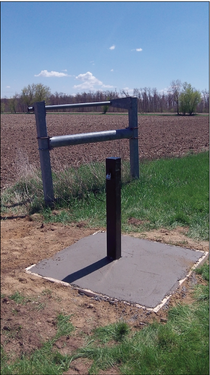
Well W2 (U.S. Geological Survey station number 421023085411201) in groundwater study area, Kalamazoo County, Michigan; photograph by Carol Luukkonen, U.S. Geological Survey.
Groundwater samples collected for this study were generally oxic (median dissolved oxygen concentration—10.16 milligrams per liter [mg/L]; 10th–90th percentiles—8.48–10.91 mg/L). Groundwaters were circumneutral to slightly alkaline (median pH—7.39; 10th–90th percentiles—7.17–7.67) and had appreciable concentrations of major ions, as indicated by specific conductance (median specific conductance—681 microsiemens per centimeter [µS/cm] at 25C; 10th–90th percentiles—571–834 µS/cm at 25C).
Surface-Water Study Area
The area selected for surface-water monitoring is in Akron Township in the northwestern part of Tuscola County (fig. 3) on the eastern side of the Lower Peninsula of Michigan. The surface-water study area is in the Pigeon-Wiscoggin watershed. Agriculture is the primary land use category with corn, soybeans, dry beans, and winter wheat being the primary crops in 2013. Soil in this study area consists mainly of Tappan Loam, which is characterized as a poorly drained loam with the potential for surface runoff ranging from negligible to high (U.S. Department of Agriculture-Natural Resources Conservation Service, 2015). These soils formed in loamy till over dense loamy till. Slopes generally range from 0 to 2 percent.
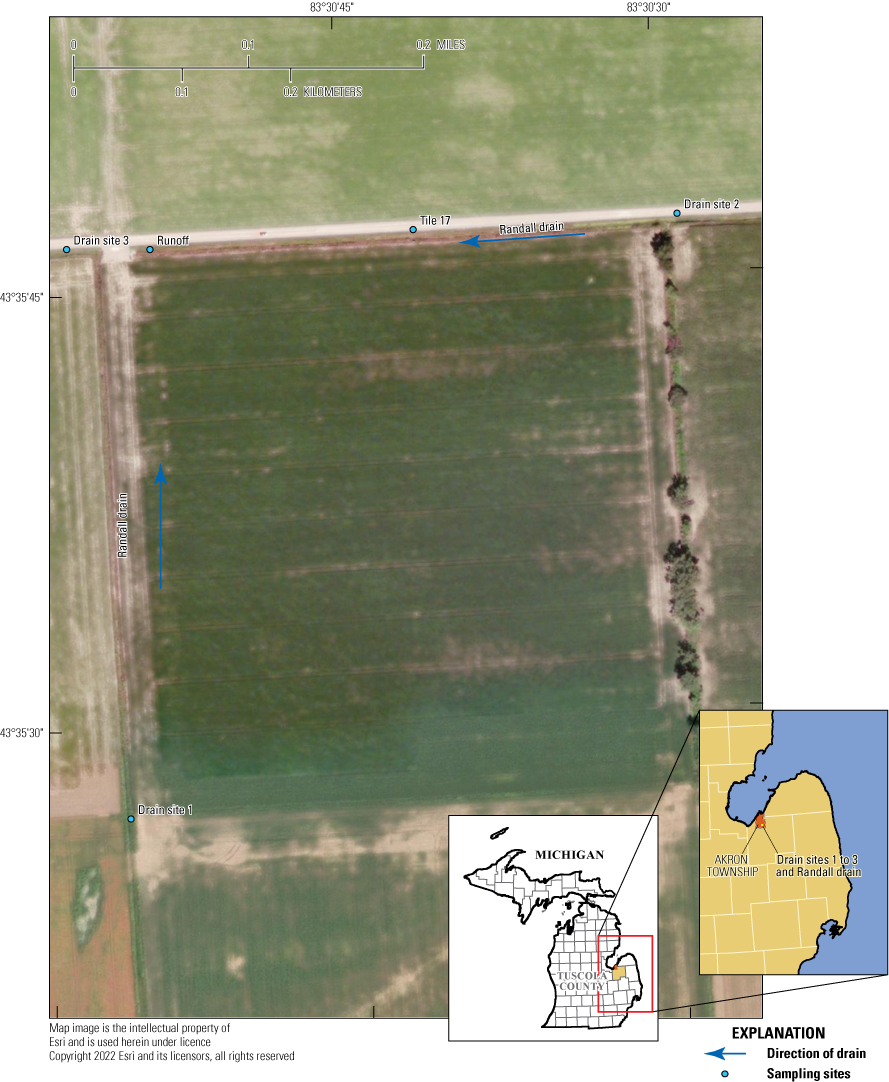
Surface-water study area and sampling sites, in Tuscola County, Michigan.
The 40 acre field was retiled in 2014 with 4 inch tiles running north and south spaced about 32 feet apart. There are 37 tiles that discharge into Randall Drain to the north and 1 tile that discharges into Randall Drain to the west just south of the driveway access. Flow in Randall Drain moves to the north along the west edge of the field and to the west along the north edge of the field. Site inspections indicated the potential for surface runoff at the northwest edge of the field along the driveway access and at an area about midway on the west side of the field. No ponds near the surface-water site were available for monitoring water quality. During the monitoring period, the cropping rotation consisted of corn during years 1, 3, and 5 (2015, 2017, and 2019) and soybeans during years 2 and 4 (2016 and 2018).
Composite automatic samplers were installed in April 2015 at one tile site and at the surface runoff area beside the driveway access to the field. The surface runoff area is where surface runoff flows into the drainage ditch during large precipitation events. At these two sites, custom-made weather resistant wood enclosures were constructed to house the samplers and additional equipment, which included a stage (water level) recorder, 12 volt deep cycle marine battery, data logger, and modem for telecommunication that enabled data acquisition and real-time programming (fig. 4). Each site also was equipped with a solar panel to assist with maintaining battery charge. At the surface runoff site, a tipping bucket rain gage was installed to measure rainfall (fig. 5). Some equipment, including samplers, batteries, dataloggers, and modems were removed from each enclosure each fall to extend equipment life and then reinstalled each spring for the start of the next monitoring season. Monitoring water quality in field and subsurface runoff consisted of sample collection at five sites throughout each growing season. Surface-water samples and flow rates at drain sites were collected at points upgradient to the field near the southwest and northeast field corners and at a point downgradient to the field at the northwest corner.
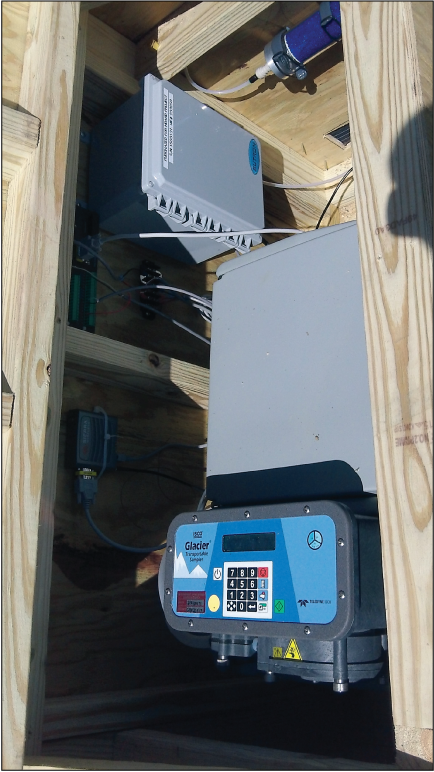
Composite automatic sampler and associated equipment at the Tile 17 site (U.S. Geological Survey station number 041572264), in the surface-water study area, Tuscola County, Michigan; photograph by Carol Luukkonen, U.S. Geological Survey.
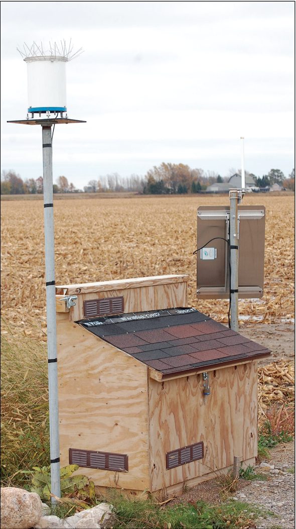
Equipment enclosure and rain gage at the runoff site (U.S. Geological Survey station number 041572269), in the surface-water study area, Tuscola County, Michigan; photograph by Julia Prokopec, U.S. Geological Survey.
The surface-water sites, when flowing, generally carried oxic waters (median dissolved oxygen concentration—9.08 mg/L; 10th–90th percentiles—4.21–12.65 mg/L). Surface waters were circumneutral to slightly alkaline (median pH—7.77; 10th–90th percentiles—7.21–8.33) and carried appreciable concentrations of major ions, as indicated by specific conductance (median specific conductance—722 µS/cm at 25 degrees Celsius; 10th–90th percentiles—323–909 µS/cm at 25 °C).
Study Design
This study was designed to investigate the potential persistence and buildup of IXF degradates in the environment near application areas. Sample collection was led at each study area over a 5-year period so that sample collection could occur during and after IXF usage. IXF was applied during the first, third, and fifth year of the study to the groundwater and surface-water study areas (table 2). The proposed number of samples and the timing of sample collection depended on IXF application frequency, prior year sampling results, site characteristics, and weather conditions. Hydrologic data including, drain flow, precipitation, and groundwater levels were collected to assist with data interpretation.
Table 2.
Crop information and 5-cyclopropyl-4-(2-methylsulfonyl-4-trifluoromethylbenzoyl) isoxazole (isoxaflutole or IXF) application dates during the study, Tuscola and Kalamazoo Counties, Michigan.[GW, groundwater; SW, surface water; IXF, 5-cyclopropyl-4-(2-methylsulfonyl-4-trifluoromethylbenzoyl) isoxazole; TCM, thiencarbazone-methyl and tembotrione]
Water Quality
Water quality is characterized using environmental and quality assurance/quality control (QA/QC) samples. Environmental samples are used to document pesticide occurrences in groundwater and surface water and QA/QC samples are used to evaluate data quality. Field and analytical methods encompass sampling procedures, equipment cleaning, and data preparation for analysis.
Environmental Samples
Each year, sample collection began in March/April before planting and herbicide application and continued until October/November after harvest from 2015 until 2019 (table 3). One set of four post-study samples was collected in 2020 at the groundwater study area. Sample collection sites included upgradient and downgradient locations. The upgradient locations were unlikely to have herbicides from the monitored fields but might show detections of herbicides if IXF was applied on other nearby fields. For example, water flowing to W1 would most likely originate from areas west of the study field.
Table 3.
Numbers of samples each year by site.[QA/QC, quality assurance/quality control]
At the groundwater study area, typically four samples were collected from each study site from 2015 to 2019. Samples were collected at three wells and at the pond once in 2020. A total of 121 environmental samples were collected at the groundwater study area.
At the surface-water study area, samples were collected from tiles, a surface runoff area, and upstream and downstream drain sites after rainfall events each year from 2015 to 2019. During the first year of the study, about 10 rainfall events were sampled to test various equipment configurations and to ensure that samples were collected from storms of varying intensities; thereafter, about 3–4 events were sampled each year. Additional periodic grab samples were collected at two additional tile sites for comparison with results from the tile sampler location during the first year. At each drain site during the fall of the third year (2017), samples were collected during base flow conditions due to a lack of sizeable rain events that would generate flow at the tile and runoff sampler locations. A total of 110 environmental samples were collected at the surface-water study area.
Field and Analytical Methods
Samples were collected using USGS standard methods (U.S. Geological Survey, variously dated). Sample collection occurred during the pre-planting/pre-application period, growing season months (generally June to August), and fall/harvest period. Sampling procedures at the drain sites consisted of collecting composite equal width-integrated samples across each section of the drain with equidistant verticals and equal transit rates within each vertical to yield a representative sample of drain condition (Shelton, 1994). Discharge flow measurements followed USGS standard procedures (Turnipseed and Sauer, 2010). Grab samples from two to three locations were collected and composited at the pond site. Groundwater samples were collected from the pump discharge tubing after purging approximately three well volumes and stabilizing field parameters (U.S. Geological Survey, 2006).
All sampling equipment was cleaned following USGS standard procedures for organic-compound sampling equipment (U.S. Geological Survey, 2004). Each 10 liter (L) glass sampler jar, Teflon bottle, and nozzle holder was cleaned and then double bagged until used. Before collecting samples at the drain or pond sites, equipment was field rinsed according to USGS standard procedures. Groundwater pump and sample tubing were cleaned before sampling and after sampling each well at the site. Composite automatic sampler tubing was cleaned each spring before sample collection and in the fall after the last sampling event for the season. During the third to fifth years of the study, the composite automatic sampler tubing was cleaned after each sampling event to minimize or eliminate the potential for carryover from one sampling event to the next.
At the surface-water study area, field measurements of pH, conductance, temperature, and dissolved oxygen were measured at three locations across the channel at each drain site or from the remainder of the water in the composite sampler jar. At the groundwater study area, field measurements of pH, conductance, temperature, and dissolved oxygen were measured using water discharged from the pump tubing at each well or from the remainder of the water in the sample jar at the pond site. All samples were filtered through a disposable 0.7 micrometer syringe tip filter (Sandstrom and Wilde, 2014). After collection and processing, samples were placed in a cooler with dry ice and shipped overnight or were stored in a deep freezer at <−10 °C until shipment to the laboratory. Samples sent to the U.S. Geological Survey National Water Quality Laboratory (NWQL) in Denver, Colorado, were analyzed for NWQL Lab Schedule 2437 pesticides (table 4) using the direct aqueous injection liquid chromatography tandem mass spectrometry method (Sandstrom and others, 2016).
Table 4.
National Water Quality Laboratory Schedule 2437 pesticides.[CASRN, Chemical Abstracts Service Registry Number; RL, reporting level; ng/L, nanograms per liter; pct, percent; OIET, 2-hydroxy-4-isopropylamino-6-ethylamino-s-triazine; CAAT, 2-Chloro-4,6-diamino-s-triazine; CEAT, 2-chloro-6-ethylamino-4-amino-s-triazine; SAA, sulfinylacetic acid; EPTC, s-ethyl dipropylthiocarbamate; RPA, Rhone-Poulenc Ag Company; MCPA, 2-methyl-4-chlorophenoxyacetic acid; DK, diketo; TP, transformation product; --, not applicable]
The NWQL detection limit (DLDQC; Bonn, 2008) is described in ASTM International’s Standard Practice D6091–07 (ASTM International, 2007) and supporting DQCALC software (Standard Practice D7510–10; ASTM International, 2010) and is now required for a laboratory to maintain National Environmental Laboratory Accreditation Conference (NELAC Institute) accreditation. The DLDQC is the lowest concentration that with 90-percent confidence will be exceeded no more than 1 percent of the time when a blank sample is measured, and there is less than a 1-percent chance of a false-positive determination. In conjunction with the DLDQC, NWQL uses a laboratory reporting level (RLDQC) set equal to (or greater than) two times the DLDQC. The probability of falsely reporting a non-detection for a sample that contains an analyte at the RLDQC concentration is predicted to be ≤1 percent.
Over the course of the study, RLDQC for some parameters in Lab Schedule 2437 were revised with limits increased for 62 compounds and decreased for 40 compounds. The RLDQC increased from 0.013 to 0.018 µg/L for IXF and from 0.009 to 0.0092 µg/L for BAA during the second year of monitoring; the RLDQC did not change for DKN during the study. The RLDQCs also were periodically increased for these three compounds due to laboratory quality assurance issues, such as instrumentation sensitivity or sample dilution. For IXF, increased RLDQCs were common: 108 of 227 samples (48 percent) had sample results reported as a non-detect at levels greater than the laboratory reporting limit of <0.013/<0.018. Sometimes, reporting levels were more than 13 times the method detection limit. For BAA, 33 of 227 samples (14 percent) and 7 of 227 DKN samples (3 percent) had reported non-detects greater than the RLDQC. These increased reporting limits may result in samples where the compound may have been present but was not quantifiable.
Quality Assurance/Quality Control Samples
Quality assurance/quality control (QA/QC) samples were collected to allow for an evaluation of data quality and a better understanding of potential errors in data results (table 5). To ensure samples are representative of environmental conditions, that cross contamination did not occur, and to document analytical variability, blank, replicate, and matrix spike samples were assessed for each study area. QA/QC samples were distributed spatially and temporally over a range of conditions to ensure adequate evaluation of the potential effects of bias and variability. Each QA/QC sample type was collected at a subset of sampling sites representing likely sources of variability and potential sources of contaminants. Analytical results for the QA/QC samples were investigated before analysis and interpretation of environmental sample data to determine data quality and whether any qualifications of the environmental concentrations were necessary. The primary compounds included in this QA/QC analysis were IXF, DKN, and BAA; however, several other frequently detected compounds were also investigated.
Table 5.
Types of quality assurance/quality control samples collected during this study, Tuscola and Kalamazoo Counties, Michigan.[NA, not applicable]
Field blanks, prepared using blank water obtained and certified to be free of target compounds by the NWQL, are intended to document the frequency and magnitude of contamination in environmental samples and are prepared so that the blank water is exposed to the potential contamination sources that might affect the environmental samples (Mueller and others, 2015). Field blank samples were analyzed to help determine whether sample collection, processing, transport, or laboratory analysis had introduced contamination from sample collection. Additionally, field blanks were used to assess whether equipment had been adequately cleaned and decontaminated before use. Field blanks were collected for the following equipment sets used during sample collection: (1) pump and tubing used for groundwater sampling, (2) 10-L glass jars and sampler tubing used in the portable automatic samplers, (3) 10-L glass jars and Teflon bottles used for pond sampling, and (4) 10-L glass jars, Teflon bottles, and nozzle holders used for drain sampling.
In a 2017 sample at the runoff site in the surface-water study area, BAA was detected in a blank sample at a concentration (0.01069 µg/L) close to the reporting level of 0.01 µg/L. IXF and DKN were not detected in any blank samples; therefore, environmental sample concentrations were not adjusted because of this one low-level detection. Source solution blanks consisting of de-ionized water produced at the Lansing, Michigan, USGS office (USGS site number 423952084321400) had no detections of any of the pesticide compounds, indicating that the water was suitable for equipment cleaning.
For the remaining pesticides, blank-sample results indicated no detections for 213 (96 percent) of the 222 constituents analyzed by the NWQL (table 6). Of the nine compounds detected in blank samples, only atrazine and tebuconazole were detected in more than one blank sample. Atrazine was detected in blank samples at the groundwater and surface-water study areas. 2-Chloro-4,6-diamino-s-triazine (CAAT), 2-chloro-4-isopropylamino-6-amino-s-triazine (CIAT), 2-hydroxy-4-isopropylamino-6-amino-s-triazine (OIAT), metalaxyl, and metolachlor SA were detected in blank samples at the groundwater study area. 2,4-dichlorophenoxyacetic acid, propoxur, and tebuconazole were detected in blank samples at the surface-water study area.
Table 6.
Summary of detections in blank samples, groundwater and surface-water study areas, Michigan.[mm, month; dd, day; yyyy, year; 2,4 D, 2,4-dichlorophenoxyacetic acid; CAAT, 2-Chloro-4,6-diamino-s-triazine; CIAT, 2-chloro-4-isopropylamino-6-amino-s-triazine; OIAT, 2-hydroxy-4-isopropylamino-6-amino-s-triazine; CO, county; W, well; <, less than; E, estimated; TRIB, tributary; MI, Michigan]
One groundwater blank sample in 2018 had six detections with four of the detected compounds much higher than the detection limit. IXF or its degradates were not detected in this instance. Inspection of the relevant compound detections in the environmental groundwater samples before and after the blank sample does not yield much information about why detections in the blank of the groundwater sampling equipment were found. In the environmental sample collected after the blank, all compound concentrations were less than the detections in the blank. Further study of these compounds would likely require some additional analyses to determine whether removal or some censoring of concentrations in wells is necessary. This blank sample appears to be anomalous because all other groundwater and surface-water blank samples had few, if any, low-level detections of pesticides, indicating low potential for contamination.
At the surface-water study area, three blanks collected in the spring indicated two compounds near the RLDQC. Atrazine was detected at concentrations less than the RLDQC in 2018 at the tile and runoff sites. Tebuconazole was detected in 2015 in a blank sample collected in the sampler glass jar at an estimated value less than the RLDQC. Tebuconazole was also detected in the tile sampler at a concentration near the RLDQC in 2019. Blanks of the surface-water sampling equipment at the pond had no compound detections.
Replicates are two or more samples that are collected, prepared, and analyzed such that they are considered to be essentially identical in composition and analysis to the original and are used to characterize the amount of variability associated with sample collection, processing, and analysis (Mueller and others, 2015). Split replicates are made from a single sample that is collected and then subdivided into other samples. Sequential replicates are made from multiple samples that are collected one after another and can help assess environmental variability within the sampled medium (Mueller and others, 2015). Replicate samples were collected to investigate whether sample collection method affected chemical concentrations in the samples (Mueller and others, 2015). After collection, both sets of samples were handled and processed identically. The relative percent difference (RPD) was calculated to compare the environmental and replicate concentrations for all sample pairs with reported concentrations in both samples.
During the study, 14 replicate samples were collected: 8 at the groundwater field and 6 at the surface-water field (table 5). Analysis of six replicate sample pairs for IXF and the DKN and BAA degradates were completed when detections occurred in the environmental and replicate samples. The reported detections used in analysis of the replicate data included two sets of sample pairs from the pond in 2019 with values assigned an “E” remark code indicating an estimated value. Concentrations for these pond samples were at about half the RLDQC. There was one pair where one sample had an estimated value and the other had no detections of the target compounds. The rest of the samples had no detections of the target compounds in the replicate and the environmental samples.
In the replicate sample pairs, the RPD was less than 15 percent for all but one pair, which had an RPD of about 22 percent. The RPDs for the tile and runoff samplers were generally lower than those for the pond samples; however, each pair was collected as a split replicate by taking two samples from the 10 L glass sampling jar. IXF was detected in one replicate pair at the runoff site with an RPD of less than 15 percent. DKN was detected in six replicate pairs from the tile sampler, runoff sampler, drain, and pond sites and had RPDs ranging from 4 to about 22 percent. Samples with smaller detected concentrations had larger RPD values. BAA was detected in the tile, runoff, and drain sites with RPDs ranging from less than 1 to 11 percent. These results were considered acceptable for the data to be used in subsequent analyses.
Matrix spikes, prepared using Lab Schedule 2437 pesticide spike solutions obtained from the NWQL, are used primarily to determine whether bias in the results was due to method performance, effects of the sample matrix, or analyte degradation during sample shipment and storage. For this study, environmental water samples collected from the field were spiked (fortified) with known concentrations of analytes (to determine recovery) and were shipped along with another environmental sample (to determine background) for analysis by the NWQL. During the first year of the project, two field spiked samples were collected at one location along with the environmental sample. The environmental sample and one spiked sample were shipped immediately for analysis, and the remaining spiked sample was stored in a deep freezer at <−10o C for about 1 month before shipment to the NWQL to evaluate potential effects on concentrations due to long-term storage beyond the recommended sample holding time. These results were used for evaluation because some samples collected during the first year of the study were stored frozen until shipment for analysis.
Matrix spike samples were collected at three wells and the pond at the groundwater field and at two drain sites, a runoff sampler site, and a tile sampler site at the surface-water field. Matrix spike results for IXF and the DKN and BAA degradates were analyzed for this study. During the first 4 years of the study (2015–18), all environmental samples that were paired with a matrix spike sample had no detections of IXF, DKN, or BAA for comparison with the spiked sample. During the fifth year (2019), both environmental samples that were paired with matrix spike samples had detections of DKN and BAA, whereas IXF was not detected in those environmental samples. Matrix spike recovery percentages were within laboratory control limits for all samples. These matrix spike results indicate that any matrix interference or analyte degradation that would affect analysis of reported sample concentrations is unlikely.
Because initial site selection was close to the time of expected product application, some samples collected during the first year (2015) of the study were stored in a deep freezer. Also, some samples were held in a deep freezer until determination of whether that precipitation event would be sampled. In 2015, 51 samples exceeded the NWQL recommended holding time of 14 days for IXF and degradates by 1 to 40 days. Of these 51, 16 samples had detectable concentrations of one or two of the target compounds. Studies completed by the herbicide manufacturer and the NWQL were consulted to determine whether the delay in analysis might create problems due to compound degradation. The NWQL data investigating the stability of the target compounds indicated mean recovery percentages ranging from 79 to 95 percent after 33 days and from 88 to 129 percent after 133 days (Duane Wydoski, NWQL written commun., 2015; Sandstrom and others, 2016). In addition, data from Bayer (Hurst, 2003) indicates negligible compound loss when samples are immediately frozen after collection and stored as long as 7 months in a deep freezer until analysis. Therefore, results from these samples were included in subsequent analyses.
Hydrologic Data
Hydrologic data collection at the surface-water study area included stage measurements at the tile and runoff sampler sites, flow measurements at the drain sites, and precipitation measurements at the runoff site. At the groundwater study area, groundwater levels were collected continuously at four wells and periodically at one well. All measurements were collected following USGS standard procedures and protocols (Shelton, 1994; Cunningham and Schalk, 2011; U.S. Geological Survey, 2022).
Temperature and precipitation data were retrieved for three weather stations (Fairgrove, Munger, and Oshtemo) from the Michigan State University Enviroweather network (Michigan State University, 2020). Fairgrove is closest to the surface-water field but had some periods of missing data; therefore, data also were retrieved for comparisons from the Munger station. Oshtemo is close to the groundwater field. Precipitation ranged from just under 20 inches to just over 40 inches per year during the study (fig. 6). Data were available for both stations since 2005 for comparison with the study period. Precipitation during the study was similar to the 2005–19 average annual precipitation at Fairgrove and generally less than 2005–19 average annual precipitation at Munger.
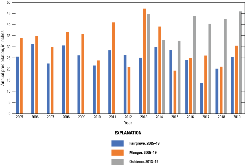
Annual precipitation from Fairgrove, Munger, and Oshtemo Enviro weather stations for the study, 2005–19, Tuscola and Kalamazoo Counties, Michigan (data from Michigan State University).
Precipitation at the groundwater field ranged from about 33 inches to just over 45 inches per year during the study based on data collected at the Oshtemo Enviroweather station (fig. 6). Data were available since 2013 for comparison with the study. Precipitation during the study was lowest in 2015 and fairly consistent for the remaining years of the study.
Data Preparation and Analysis
Data used in this report were retrieved from the USGS National Water Information System database (U.S. Geological Survey, 2022) and processed before analysis. All estimated values, with an “E” remark code, were considered valid results. Of the 227 environmental samples, four post-study samples collected in 2020 at the groundwater study area had no detections of IXF compounds and are not included in subsequent analyses.
Boxplots were used to graphically show compound concentrations and how these concentrations varied over the course of the study. Boxplots show the center of the data (median) by the centerline of the box, the variation or spread (interquartile range) by the height of the box, the skewness (quartile skew) by the relative size of the halves of the box, and the presence or absence of outliers or unusual values by the lines and points extending from each side of the box (Helsel and others, 2020).
For comparisons, data were grouped according to the time of year the sample was collected. For application years, the time before or after application was used to group samples as follows: (1) pre-application—samples collected before IXF application (April or May); (2) post-one-month—samples collected about one month after IXF application after the first major precipitation event (June); (3) post-late-summer—samples collected in late summer (July, August, or September), generally 2–3 months after IXF application; and (4) post-fall—samples collected in fall generally after fields were harvested (October or November). For non-application years, samples were grouped according to time of year: (1) early spring (April or May), (2) early summer (June), (3) late summer (August), and (4) fall (October or November). When some analyses had more than one sample in a time interval for a given year, the sample closest in time to samples in a previous or subsequent year was selected and included in the comparisons.
All statistical tests were evaluated at probabilities (p-values) of less than 0.05 (p<0.05) to be considered significant. Statistical analysis was completed in R (R Core Team, 2014), and most figures were produced using the package ggplot2 (Wickham, 2009). Statistical methods for censored data included in the NADA R package were used for all analyses (Helsel and Lee, 2006). The cenfit command compares an estimate of an empirical cumulative distribution function for datasets that include censored data using the Kaplan-Meier method. The cendiff command tests if there is a difference between two or more empirical cumulative distribution functions using the nonparametric Peto-Prentice test as described in Helsel and Lee (2006). Statistical methods for censored data included in the smwrQW package were used for testing for differences among three or more groups. The censMulticomp test performs multiple comparison tests for censored data by running repeated generalized Wilcoxon tests among all groups as described in Helsel (2012). DKN and BAA results among these groups of data were compared using the generalized Wilcoxon test (Helsel, 2012) as implemented in the smwrQW package for R statistical software (Lorenz, 2016); this test handles datasets that include left-censored data.
Field dissipation rate constants were determined for DKN and BAA using concentration time series data from the surface-water sites, starting with post-application maximum concentrations. This analysis was done for sites with 2 to 9 samples that had detectable concentrations of DKN and BAA. First-order field dissipation rate constants were defined as the slope of a linear regression of the natural logarithm of concentration versus time, in days, from the maximum post-application concentration, using linear regression.
Results and Discussion
Sample analysis results were evaluated from different perspectives due to the number and variety of sampling sites. Initial evaluations investigated the presence or absence of the target pesticide IXF and its degradates based on source of water, whether groundwater or surface water. Other information, such as groundwater levels, was evaluated, as well as concentrations for other non-target pesticides that were detected most often. For surface water, which had more frequent detections of IXF and its degradates, chemical concentrations, IXF application date, and gage height are plotted as time series plots. Next, concentration data were grouped by season, across years for application years, and by season for non-application years, to view the data in summary form and to examine differences among seasons.
Groundwater
Water levels were measured continuously at wells W2, W3, W4, and W5 and periodically at well W1 (fig. 7) during the study except for a few periods when water levels were not measured continuously due to equipment issues. Water levels in W1, W2, and W5 were consistently higher than levels in W3 and W4, indicating that groundwater flow directions are towards the southeast. During spring and summer, water levels in W2 were lower than in W1 and W5. Because W2 is near an irrigation well, available data on irrigation pumping were requested for 2017 and 2018. Water levels in W2 decreased in response to nearby pumping and, to a lesser extent, downgradient W3 and W4 showed a similar effect.
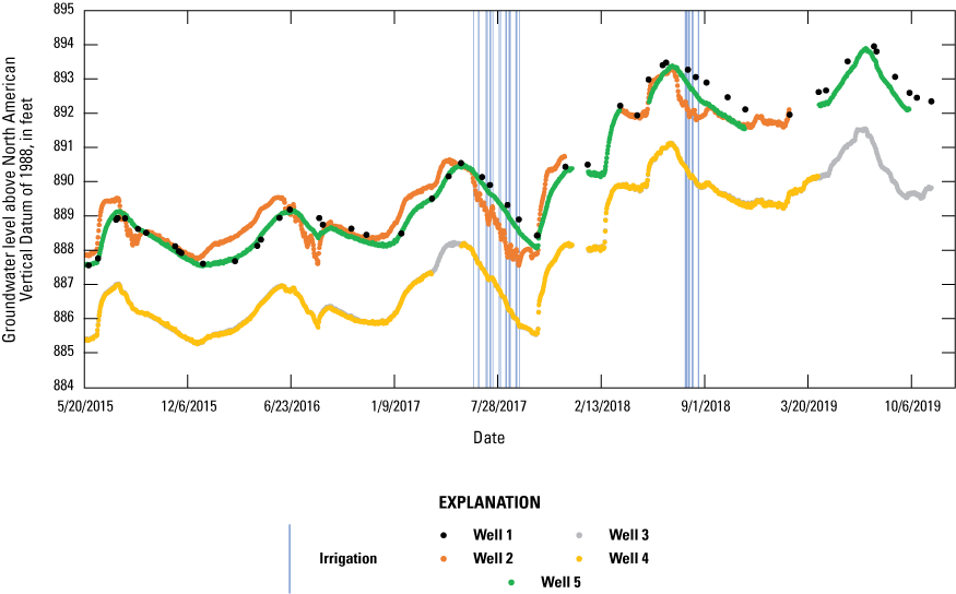
Groundwater levels for 2015 to 2019 and irrigation pumping for 2017 and 2018, in the groundwater study area, Kalamazoo County, Michigan.
During the study, 57 groundwater samples were collected from the 5 wells during application years and 40 samples from non-application years. In these samples, only one detection of a target compound was reported: DKN was reported as an estimated concentration at W1 in late summer 2017. W1 was upgradient to the study field, so potentially this well was affected by IXF application to a neighboring field. These findings agree with other findings from studies in Nebraska, Iowa, and Indiana where IXF and its degradates were not detected or rarely detected in groundwater (Bayer CropScience, 2004).
Surface Water
Monthly precipitation totals were compared with average monthly precipitation from 2005 to 2019 using the Michigan State University Enviroweather Stations at Fairgrove and Munger data (fig. 8). In July and early August 2018, the onsite rain gage was damaged; therefore, for this period, data from the Fairgrove station was used to fill in missing rain gage data. For May and July, onsite precipitation was generally at or below historical median amounts. For August and October, onsite precipitation was generally at or above historic median amounts. Onsite precipitation for June and September was more variable in relation to historical median amounts. IXF application dates and target compound analytical results were compared to stage measurements each year at the tile and runoff sampler sites (figs. 9–12). Figures 9 and 10 illustrate sampling dates, application dates, time since application, and gage heights at the tile site (USGS station 041572264) and runoff site (USGS station 041572269), respectively, during application years. Figures 11 and 12 illustrate sampling dates and gage heights at these sites during the years when IXF was not applied.
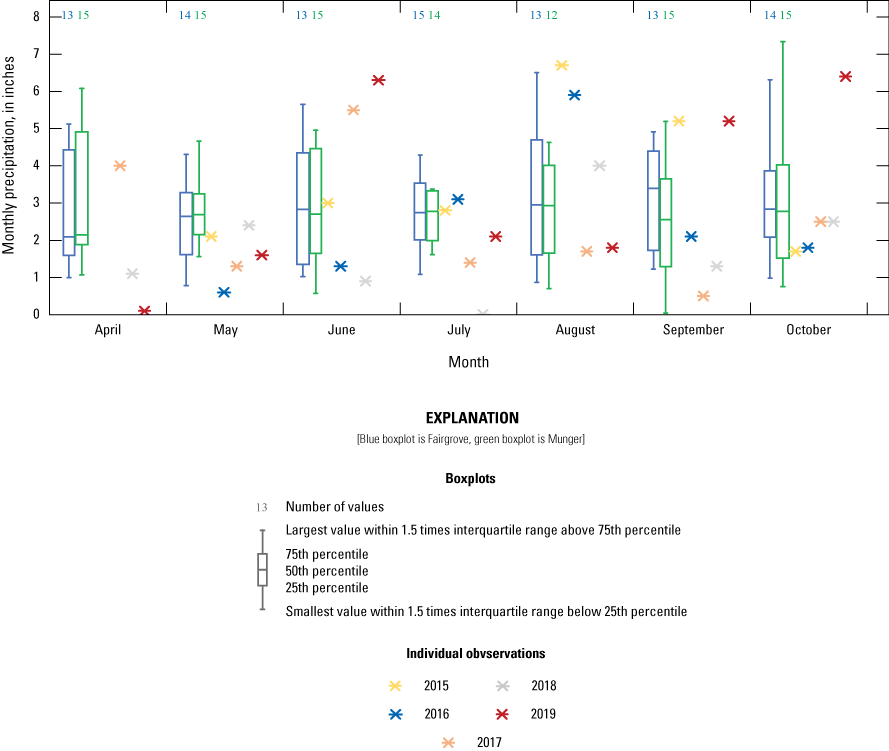
Monthly precipitation from the 2005 to 2019 growing seasons for the Fairgrove and Munger Enviro-weather stations and from 2015 to 2019 for the rain gage at U.S. Geological Survey station 041572269, Tuscola County, Michigan.
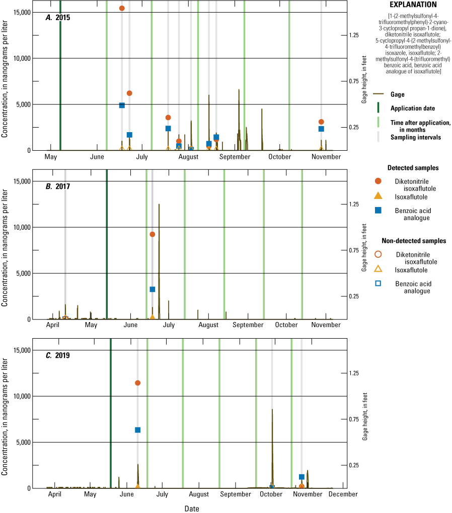
Concentration of 5-cyclopropyl-4-(2-methylsulfonyl-4-trifluoromethylbenzoyl) isoxazole (isoxaflutole), its degradates 2-methylsulfonyl-4-(trifluoromethyl) benzoic acid (benzoic acid analogue of isoxaflutole) and 1-(2-methylsulfonyl-4-trifluoromethylphenyl)-2-cyano-3-cyclopropyl propan-1-dione) (diketonitrile isoxaflutole), and gage height at the runoff site during tributary application years: A, 2015; B, 2017; and C, 2019.
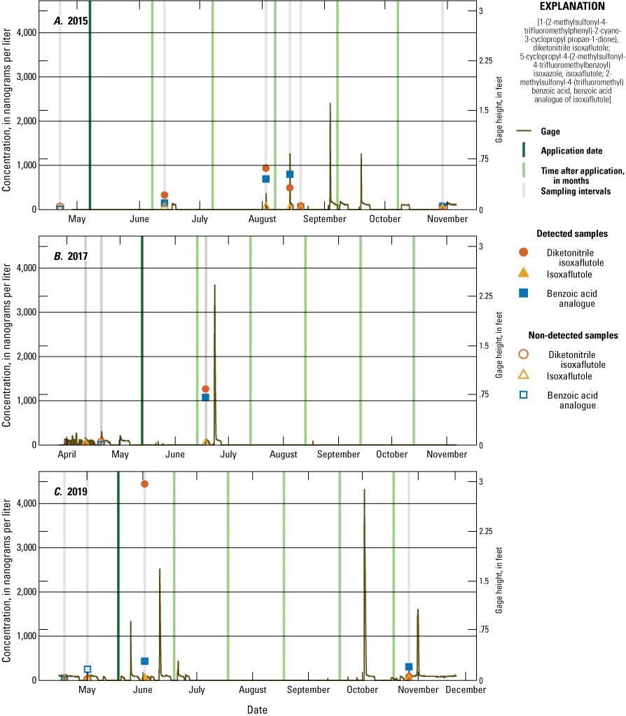
Concentration of 5-cyclopropyl-4-(2-methylsulfonyl-4-trifluoromethylbenzoyl) isoxazole (isoxaflutole), its degradates 2-methylsulfonyl-4-(trifluoromethyl) benzoic acid (benzoic acid analogue of isoxaflutole) and 1-(2-methylsulfonyl-4-trifluoromethylphenyl)-2-cyano-3-cyclopropyl propan-1-dione) (diketonitrile isoxaflutole), and gage height at the tile sampler site during tile application years: A, 2015; B, 2017; and C, 2019.
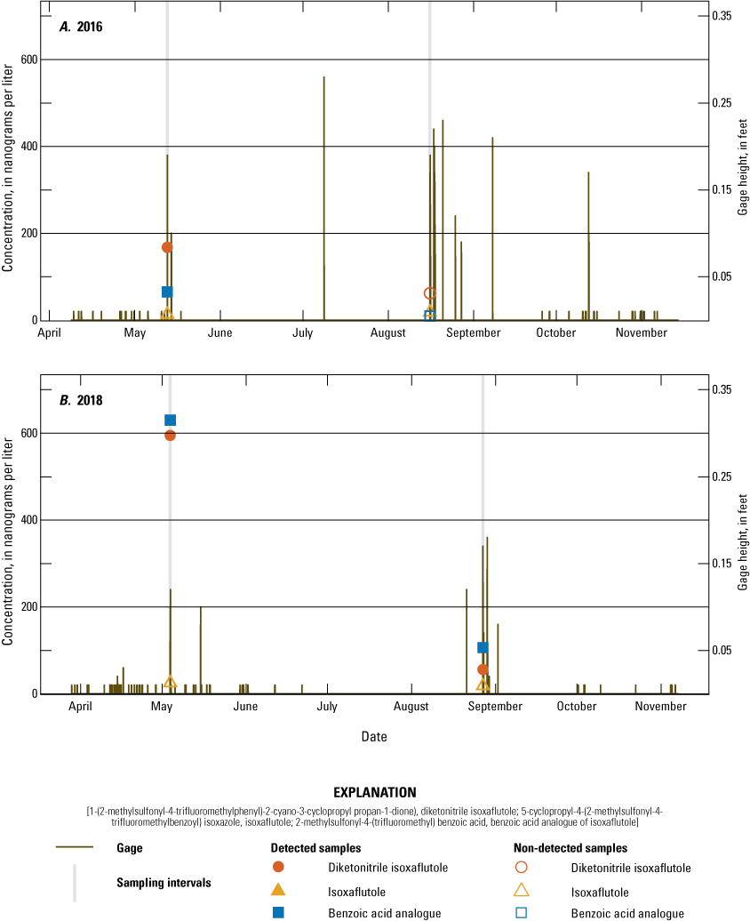
Concentration of 5-cyclopropyl-4-(2-methylsulfonyl-4-trifluoromethylbenzoyl) isoxazole (isoxaflutole), its degradates 2-methylsulfonyl-4-(trifluoromethyl) benzoic acid (benzoic acid analogue of isoxaflutole) and 1-(2-methylsulfonyl-4-trifluoromethylphenyl)-2-cyano-3-cyclopropyl propan-1-dione) (diketonitrile isoxaflutole), and gage height at the runoff sampler site during tributary non-application years: A, 2016 and B, 2018.
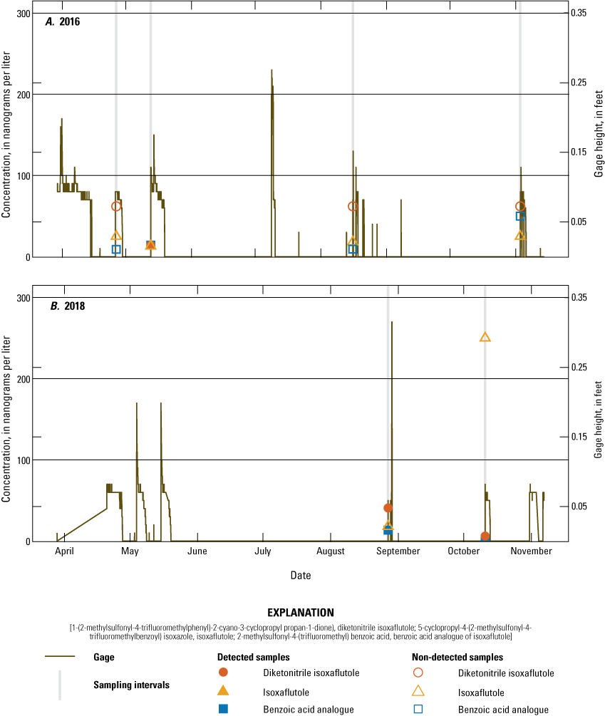
Concentration of 5-cyclopropyl-4-(2-methylsulfonyl-4-trifluoromethylbenzoyl) isoxazole (isoxaflutole), its degradates 2-methylsulfonyl-4-(trifluoromethyl) benzoic acid (benzoic acid analogue of isoxaflutole) and 1-(2-methylsulfonyl-4-trifluoromethylphenyl)-2-cyano-3-cyclopropyl propan-1-dione) (diketonitrile isoxaflutole), and gage height at the tile sampler site during tile non-application years: A, 2016 and B, 2018.
Over the course of the study, 126 surface-water samples were collected from the tile sampler, runoff sampler, drains, and pond. One or more of the three target IXF compounds were detected in 51 (40 percent) samples with detections in 40 of 90 (44 percent) samples in application years and detections in 11 of 36 (31 percent) surface-water samples from non-application years. During the growing season (June–August, each year), one or more of the three target IXF compounds were detected in 35 of 68 (51 percent) samples in application years and 6 of 24 (25 percent) samples in non-application years. IXF was in three samples, one in 2017, 36 days post-application, and two in 2019, 15 and 23 days post-application. The IXF detection in 2017 was from the tile sampler, and the detections in 2019 were from the tile and runoff samplers (figs. 9 and 10). All three of the samples containing IXF also had DKN and BAA. The infrequent detection of IXF agrees with other studies in Ohio, Iowa, and Indiana (Bayer CropScience, 2004) and can be explained by the fact that IXF rapidly degrades to DKN under normal field conditions. DKN was detected in 33 surface-water samples collected during application year growing seasons and 5 surface-water samples collected during non-application year growing seasons. BAA was detected in 29 surface-water samples collected during application year growing seasons and 4 surface-water samples collected during non-application year growing seasons. The maximum number of detections occurred within 1 month of application. Maximum concentrations for all three compounds occurred during application years within 1 month of application. The maximum concentrations of IXF, DKN, and BAA were 0.108 µg/L, 15.4 µg/L, and 6.33 µg/L, respectively.
Twenty-one surface-water samples were collected from drain site 1, which is upgradient to the surface-water field. IXF or its degradates were not detected in any of these samples. Drain site 2 is also upgradient to the surface-water field and had 4 detections in 23 samples: 3 detections being DKN and 1 detection being BAA. All four detections were at concentrations less than the RLDQC. Two detections of DKN were in samples collected before IXF application in 2015 and may indicate indirect impacts of IXF application to a neighboring field. DKN was also detected in late summer 2016, and BAA was detected in a sample about one month after application in 2019. These low-level detections indicate IXF or its degradates can be transmitted from off-site sources. Therefore, subsequent analyses will focus on the remaining downgradient surface-water sampling sites where constituent concentrations can be related to onsite applications.
DKN and BAA results for drain site 3, tile sampler, runoff sampler, and the pond were compared for years with IXF application (2015, 2017, and 2019) and years without IXF application (2016 and 2018) (fig. 13). The RLDQC is shown as a dashed line on each plot; however, many samples were affected by raised reporting levels. With only three detections for IXF, no boxplots were created. IXF degradate concentrations have highest concentrations after pesticide application but decrease during summer, fall, and into the following year. During the non-application years, concentrations were generally highest during the early spring and decreased throughout the year; concentrations were generally lower than during application years. These patterns are similar to patterns observed in other studies (for example, Scribner and others, 2006).
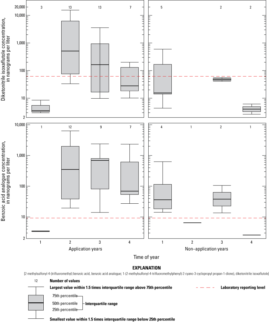
Boxplots showing 1-(2-methylsulfonyl-4-trifluoromethylphenyl)-2-cyano-3-cyclopropyl propan-1-dione) (diketonitrile isoxaflutole) and 2-methylsulfonyl-4-(trifluoromethyl) benzoic acid (benzoic acid analogue of isoxaflutole) concentrations during the growing season of application and non-application years, for the pond, tile, runoff, and drain site 3 sampling sites, Kalamazoo and Tuscola Counties, Michigan.
DKN and BAA concentrations at the pond, tile sampler, runoff sampler, and drain site 3 for each application year were compared to determine whether evidence of increasing concentrations over time could be determined. Concentrations generally follow a repeatable pattern during each of the application years: lowest concentrations are in the pre-application samples, highest concentrations are within about 1 month after IXF application, and decreasing concentrations follow in the late summer and fall samples. All distributions of DKN and BAA concentrations within a given season and by application year were similar (figs. 14 and 15), showing no significant differences (Wilcoxon Peto-Prentice test, p>0.05) in all cases. Similarly, during the non-application years, concentrations within a given season did not significantly differ across years (figs. 14 and 15), when sufficient data to run the Peto-Prentice test were available.
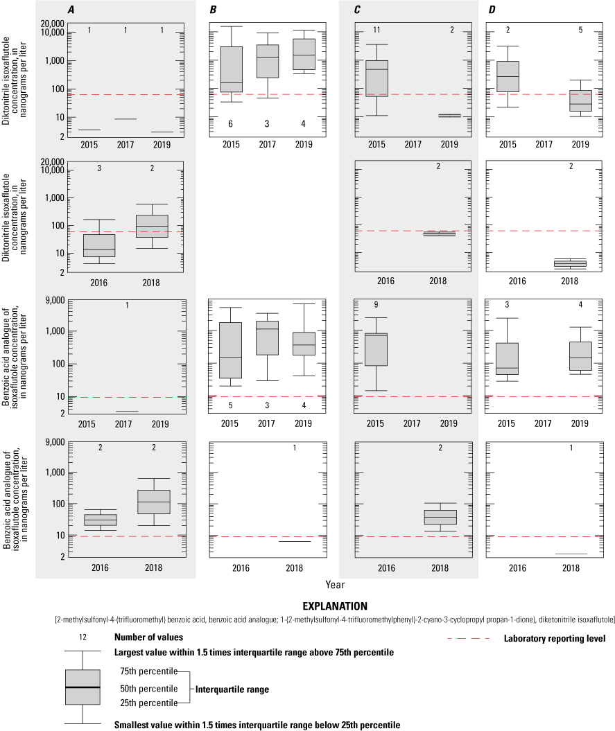
Boxplots showing 1-(2-methylsulfonyl-4-trifluoromethylphenyl)-2-cyano-3-cyclopropyl propan-1-dione) (diketonitrile isoxaflutole) and 2-methylsulfonyl-4-(trifluoromethyl) benzoic acid (benzoic acid analogue of isoxaflutole) concentrations during the growing season by year for the pond, tile, runoff, and drain site 3 sampling sites, Kalamazoo and Tuscola Counties, Michigan. A, early spring/pre-application; B, early summer/post 1 month; C, late summer/post late summer; D, fall/post fall (shading used to show column groups).
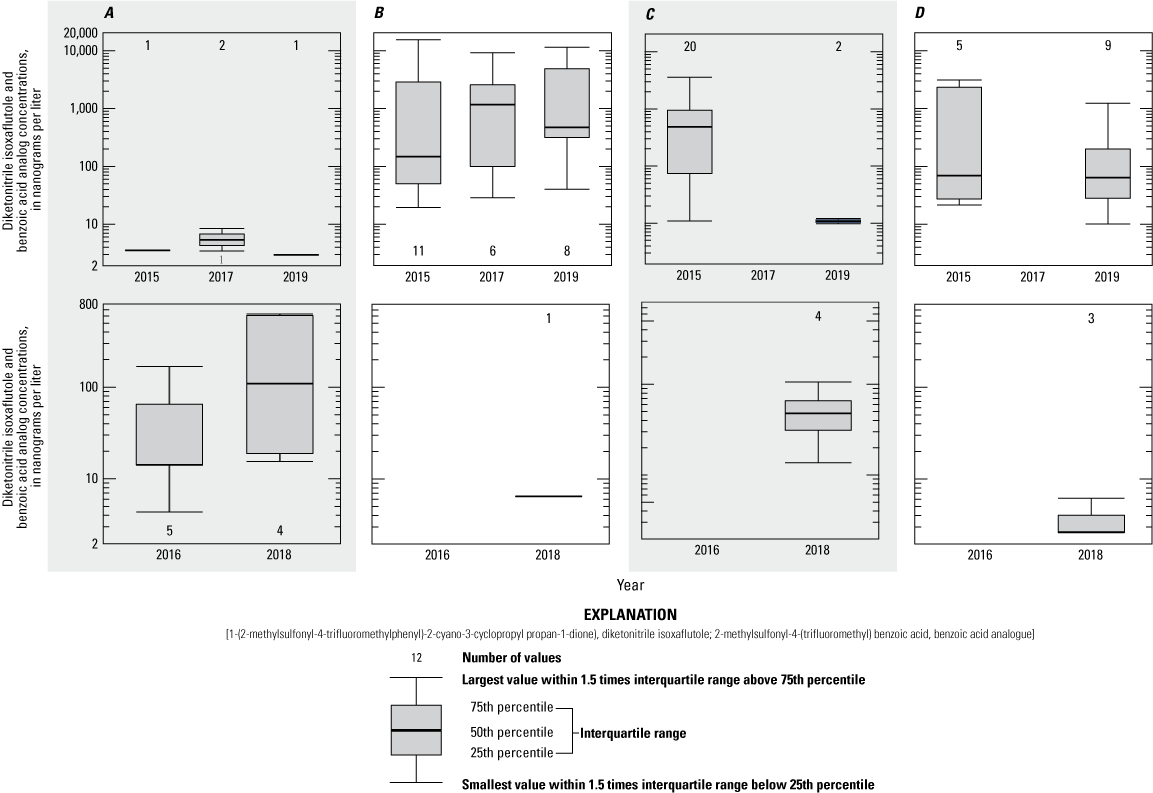
Combined 1-(2-methylsulfonyl-4-trifluoromethylphenyl)-2-cyano-3-cyclopropyl propan-1-dione) (diketonitrile isoxaflutole) and 2-methylsulfonyl-4-(trifluoromethyl) benzoic acid (benzoic acid analogue of isoxaflutole) concentrations for growing season time intervals for application and non-application years, for the pond, tile, runoff, and drain site 3 sampling sites, Kalamazoo and Tuscola Counties, Michigan. A, early spring/pre-application; B, early summer/post 1 month; C, late summer/post late summer; D, fall/post fall (shading used to show column groups).
The pre-application season during application years is considered a baseline sampling period; that is, the period when concentrations are expected to be lowest. For surface-water sites, DKN and BAA concentrations from subsequent sampling periods were compared with the pre-application concentrations. Water samples were binned according to season as follows: 1-month post-application, late summer post-application, fall post-application, and non-application years (all seasons). DKN results were significantly greater in the 1-month post-application (p<0.05) and late summer (p<0.05) seasons compared with pre-application concentrations. Similarly, BAA concentrations were significantly greater in the 1-month post-application (p=0.0016) and fall (p=0.027) seasons compared with pre-application concentrations. DKN results in the fall (p<0.10) season and BAA results in the late summer (p=0.075) season were above the significance level but do indicate a difference between application and non-application years. Concentrations of DKN and BAA from pre-application season were similar (p>0.1) to concentrations observed during the non-application year's samples. Although low concentrations of these compounds occurred in some spring samples during non-application years (figs. 11–14), too few samples with detectable concentrations were available to compare single non-application-year seasons statistically; therefore, all non-application-year seasons were combined for this analysis.
Given the observed high concentrations of DKN and BAA, followed by decreases in concentrations over a time scale of a growing season to about 1-year post-application, DKN and BAA concentrations were examined in the context of field dissipation rates using principles of first-order kinetics. In this report, field dissipation rates describe the decrease in concentrations over time, after post-application maxima, at the surface-water sites where DKN and BAA were detected. Mechanisms for the decreases in concentrations are thought to include microbial degradation and flushing (that is, advective transport from the fields via surface runoff), whereas other potential mechanisms (volatilization, photodegradation) are thought to be minor (Bayer CropScience, 2004). Papiernik and others (2007) found uptake by plants to be an important mechanism for IXF dissipation in Minnesota. The relative importance of microbial degradation versus flushing cannot be ascertained from our data, and the field dissipation rate constants and half-lives should not be thought of as degradation rates.
From first-order kinetics, the concentration of a substance at time t (Ct) is given by: Ct=C0 ekt, where C0 is the concentration at time = 0, and k is the rate constant. Linear regression of the natural logarithm of observed concentration versus time yields a slope, which is the rate constant k. Negative slope (k) indicates degradation or loss of a chemical. For this analysis, C0 is defined as the maximum observed concentration after the application of IXF, and time is the time (in days) after the maximum observed concentration. For this analysis, rate constants are reported as kdiss (units in day−1) and half-lives are reported as t1/2, diss (units in days) (the diss subscript is used to distinguish dissipation rates from reaction rates, including degradation reactions).
Within surface-water sites with two to eight sequential, detectable concentrations of DKN or BAA (including estimated results below the RLDQC) after application, kdiss and t1/2, diss were determined for each series of data. As the data allow, based on timing of sampled runoff events after application, three periods were considered: (A) growing season post-application maximum to late summer; (B) medium period, post-application maximum to fall; and (C) long period, post-application maximum into the following year. Table 7 lists the time series considered for each of these periods, and reports the kdiss and t1/2, diss values obtained from this analysis.
Table 7.
Field dissipation constants and half-lives for 1-(2-methylsulfonyl-4-trifluoromethylphenyl)-2-cyano-3-cyclopropyl propan-1-dione) (diketonitrile isoxaflutole or DKN) and 2-methylsulfonyl-4-(trifluoromethyl) benzoic acid (the benzoic acid analogue of isoxaflutole or BAA).[Data from the National Water Information System. DKN, diketonitrile isoxaflutole; BAA, benzoic acid analogue of isoxaflutole; N, number; kdiss, rate constants; t1/2, diss, half-lives; Trib, tributary; NA, not applicable]
The fastest dissipation rates were observed during the growing season, with a median t1/2, diss of 13.4 days and 24.3 days for DKN and BAA, respectively. For the medium period, a median t1/2, diss of 22.3 days and 48.2 days for DKN and BAA, respectively, was observed, and for the long period, a median t1/2, diss of 79.2 days and 70.6 days for DKN and BAA, respectively, was observed. Because microbial degradation rates are temperature dependent, the observation of longer dissipation half-lives (slower dissipation rate constants) is to be expected in the medium and long periods, because colder (and drier conditions with low runoff) seasons are included in those periods.
For comparison, Bayer CropScience (2004) reports dissipation half-lives for four U.S. field soils as follows: IXF—1.8–2.7 days; DKN—6.5–79 days; and BAA—5.6–61 days. The longer half-lives for DKN and BAA were reported for a field site in California, which likely is considerably different in hydroclimatic and soil conditions from the other field sites. Field studies in Nebraska, Washington, and North Carolina (Bayer CropScience, 2004) yielded remarkably similar dissipation half-lives to the surface-water sites in this study. Dissipation kinetics of the parent compound, IXF, were not analyzed in this report because nearly all samples did not have detectable concentrations. Median dissipation half-lives for DKN (8.9 days) and BAA (22 days) from the Bayer CropScience studies are similar to dissipation half-lives determined for the growing season in this study.
The data (figs 13–15) show carryover of DKN and BA from one growing season to the next; however, the level of carryover is very low, and loss mechanisms would be expected to continue during the following growing season. To put the pseudo-first order loss constants into perspective, kdiss=−0.05 day−1 would result in 99-percent loss of an initial concentration within 92 days, whereas kdiss=−0.01 day−1 would result in 99-percent loss within 460 days [note: 99-percent loss of a starting concentration of 1.0 is 0.01; ln(0.01)/−kdiss=t.].
The regression-based calculations of field dissipation rate constants and half-lives in this report only used detected concentration data. We acknowledge that ignoring non-detect (<RLDQC) data biases the results. However, application of more robust statistical techniques such as maximum likelihood regression was not attempted, given the low numbers of samples for each time series (n=2–9).
Other Pesticides
In addition to IXF and its principal degradates, DKN and BAA, a secondary focus of this study was to document 223 additional pesticides consisting of herbicide, fungicide, and insecticide parent compounds and degradates. Compounds other than IXF are summarized in this section to complete the picture of groundwater and surface-water conditions at the field sites. Of the 223 pesticides, 81 were detected at least once: 23 were detected in groundwater, 77 were detected at the surface-water field site, and 41 were detected in the pond at the groundwater site. Of these 81 only 49 were detected 5 or more times. Eighteen pesticides were detected in all three areas. Oxamyl oxime, sulfometuron methyl, and hexazinone TP G were detected solely in groundwater samples. Sulfentrazone was detected solely in surface water at the pond. Thirty-five pesticides were detected solely at the surface-water field site.
Atrazine (and its degradates CAAT, CIAT, OIAT, and OIET; see table 4) and metolachlor (and its degradates metolachlor OA and SA; table 4) were detected most frequently (fig. 16). Out of 227 samples, atrazine was detected in 164 samples (72 percent) and concentrations ranged from 0.0012 to 439 µg/L. The highest atrazine concentrations were observed in surface-water samples from the tile and runoff site after rainfall after product application and at the pond the year after product application. Metolachlor was detected in 111 samples (49 percent) and concentrations ranged from 0.0011 µg/L to 2 µg/L. The highest concentration of metolachlor was from a pond sample at the groundwater study area. Atrazine was in groundwater samples and surface-water samples from both study areas and the pond, whereas metolachlor was found only in surface samples and the pond samples. Metolachlor SA was detected most frequently (191 samples out of 227, 84 percent) and concentrations ranged from 0.015 µg/L to 11.6 µg/L. Highest concentrations were generally observed during the first year of the study (2015) and were often highest in one of the upgradient drain sites (drain site 1 and drain site 2). CAAT, CIAT, OIAT, and OIET were observed in 153 (67 percent), 190 (84 percent), 149 (66 percent), and 150 (66 percent) groundwater and surface-water samples, respectively. Metolachlor OA was observed in 110 (48 percent) groundwater and surface-water samples.
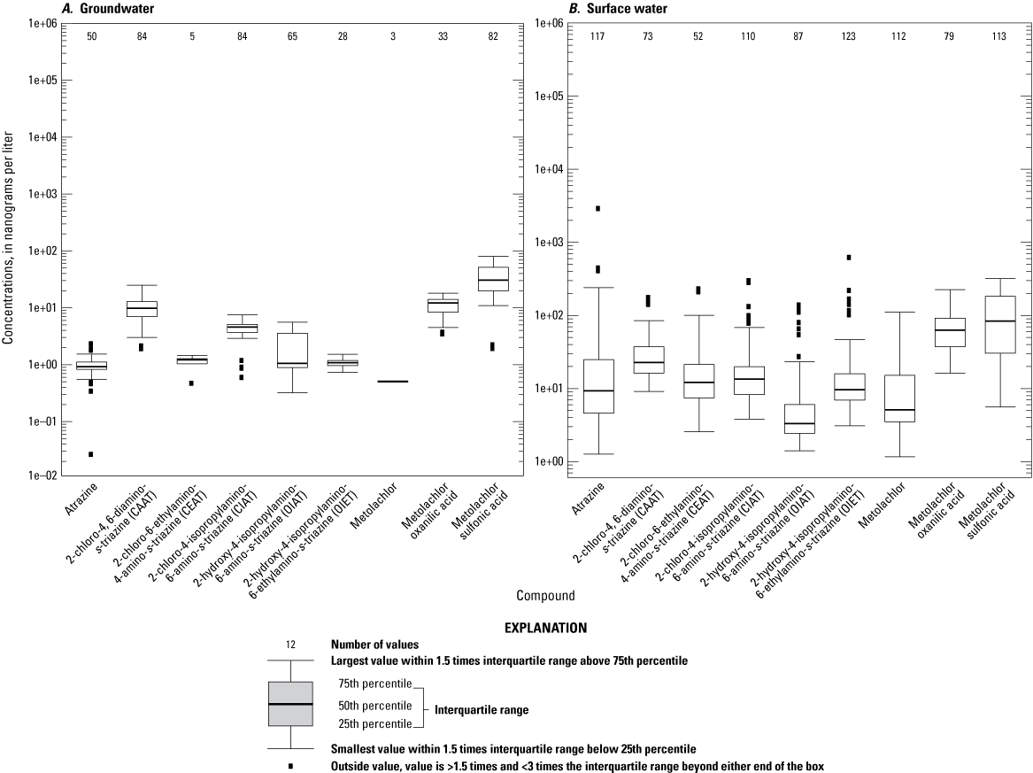
Atrazine, atrazine degradate, metolachlor, and metolachlor degradate concentrations in A, groundwater and B, surface water in Kalamazoo and Tuscola Counties, Michigan.
Summary and Conclusions
The herbicide 5-cyclopropyl-4-(2-methylsulfonyl-4-trifluoromethylbenzoyl) isoxazole] (IXF or isoxaflutole) was conditionally approved for use on corn in Michigan in 2015. Many studies have been completed to assess the fate of IXF residues and its degradates in different environmental settings and the processes by which these compounds move to groundwater or to surface-water bodies. Due to the different soil and climate conditions in Michigan, as compared to other areas where this herbicide has been used, little information about possible persistence and buildup of this herbicide and its metabolites in Michigan’s groundwater and surface water is available. Therefore, from 2015 to 2020, the U.S. Geological Survey, in cooperation with the Michigan Department of Agriculture and Rural Development, studied IXF and two of its degradates in two locations where IXF was applied. This is the only study having more than one IXF application and with the varied soil conditions in Michigan. The secondary objective of this study was to document other commonly used pesticides in Michigan.
Shallow groundwater sampling sites downgradient of IXF applications showed virtually no IXF or degradate contamination. One or more of the three target IXF compounds were detected in 40 percent of surface-water samples. The degradates 1-(2-methylsulfonyl-4-trifluoromethylphenyl)-2-cyano-3-cyclopropyl propan-1-dione) (diketonitrile isoxaflutole or DKN) and 2-methylsulfonyl-4-(trifluoromethyl) benzoic acid (benzoic acid analogue of isoxaflutole or BAA) were detected more frequently than the parent compound. For each of the surface-water sites, DKN and BAA reached maximum concentrations within about the first 5 weeks of IXF application and were associated with rainfall-runoff events. Subsequent to post-application maxima, concentrations decreased through time approximately following first-order, exponential loss kinetics. Carryover of DKN and BAA, from an application year to the following spring, was observed at several surface-water sites, with springtime concentrations typically 1–5 percent of maximum, post-application concentrations, and virtually no detections later in the growing season during non-application years. Results indicate rapid loss of IXF from the study areas and very few detections of the parent compound. The degradates DKN and BAA were more frequently detected and were detected in surface runoff up to about 1 year after IXF application, with no evidence of longer-term buildup of concentrations in the study areas.
Neither IXF nor its degradates were observed in the shallow groundwater system when samples were taken from downgradient wells after application of IXF. In the surface waters studied, IXF was rarely detected and only detected at low concentrations within about 5 weeks of application. Based on the observed patterns of IXF concentrations and its two degradates, DKN and BAA, we made several conclusions.
-
• DKN and BAA in surface-water samples after IXF application, except for very few, low-concentration detections of IXF, indicate relatively fast degradation of the parent compound in surficial soils and surface waters.
-
• Observed maximum concentrations of the degradates DKN and BAA decrease over time scales of months to 1-year post-application. By the end of an application year’s growing season, DKN and BAA concentrations typically were approximately 1–5 percent of maximum, post-application concentrations. Where detected, similar concentrations (1–5 percent of maximum) occurred in early spring surface-water samples in the year after an application year; however, by mid-summer in a non-application year, DKN and BAA typically were not detectable. The data show no buildup of IXF or its degradates over multi-year time scales at the sampled surface-water sites.
In addition, samples from 2015 to 19 were analyzed for approximately 223 additional pesticides consisting of herbicide, fungicide, and insecticide parent compounds and degradates. Of the 223 pesticides, 81 were detected at least once with 23 detected in groundwater, 77 detected at the surface-water field site, and 41 detected in the pond at the groundwater site. Of these 81, only 49 were detected 5 or more times. Atrazine and several of its degradates and metolachlor and two of its degradates were detected most frequently. Out of 227 samples, atrazine was detected in 164 samples (72 percent), and concentrations ranged from .0012 to 439 micrograms per liter (µg/L). The highest atrazine concentrations were observed in surface-water samples from the tile and runoff sites after rainfall events and product application and at the pond the year after product application. Metolachlor was detected in 111 samples (49 percent), and concentrations ranged from 0.0011 µg/L to 2 µg/L.
Study Limitations
These conclusions do have key limitations that should be recognized. First, the conclusions should not be extrapolated to settings that differ markedly in soil type, hydrogeologic conditions, water chemistry, and other key environmental conditions from those of this study. Second, underlying mechanisms behind the decreases in concentrations after application were beyond the scope of this study; microbial degradation pathways and advective pathways (flushing from the fields via runoff, and loss through surface water and groundwater transport) are likely factors, but the relative importance cannot be assigned to these mechanisms. Finally, more precipitation events and subsequent sample collection during non-application years would have assisted with interpretation of IXF and degradate behavior after application. Additional samples during application and non-application years would help improve these assessments and reduce uncertainty in stated conclusions.
References Cited
Battaglin, W.A., Thurman, E.M., Kalkhoff, S.J., and Porter, S.D., 2003, Herbicides and tansformation products in surface waters of the midwestern United States: Journal of the American Water Resources Association, v. 39, no. 4, p. 743–756. [Also available at https://doi.org/10.1111/j.1752-1688.2003.tb04402.x.]
Bonn, B.A., 2008, Using the U.S. Geological Survey National Water Quality Laboratory LT-MDL to evaluate and analyze data: U.S. Geological Survey Open-File Report 2008–1227, 79 p. [Also available at https://doi.org/10.3133/ofr20081227.]
Goolsby, D.A., Thurman, E.M., and Kolpin, D.W., 1991a, Geographic and temporal distribution of herbicides in surface waters of the upper Midwestern United States, 1989–90, in Mallard, G.E., ed., U.S. Geological Survey toxic substance hydrology program—Proceedings of the technical meeting, Monterey, California, March 11–15, 1991: U.S. Geological Survey Water-Resources Investigation Report 91–4034, p. 183–188. [Also available at https://doi.org/10.3133/wri914034.]
Helsel, D.R., Hirsch, R.M., Ryberg, K.R., Archfield, S.A., and Gilroy, E.J., 2020, Statistical methods in water resources: U.S. Geological Survey Techniques and Methods, book 4, chap. A3, 458 p. [Also available at https://doi.org/10.3133/tm4A3.]
Helsel, D., and Lee, L., 2006, Analysis of environmental data with nondetects—Statistical methods for censored environmental data: Continuing Education Workshop at the Joint Statistical Meetings, Seattle, Wash., accessed June 7, 2021, at https://www.practicalstats.com/resources/NADA-resources/NADAforR_Examples.pdf.
Lorenz, D.L., 2020, smwrQW-package: Tools for censored water-quality data analysis, accessed July 2021, at https://rdrr.io/github/USGS-R/smwrQW/man/smwrQW-package.html
Michigan Department of Environment, Great Lakes, and Energy, 2015, GeoWebFace: State of Michigan digital data, accessed December 2016, at http://www.deq.state.mi.us/geowebface/.
Michigan Farm Bureau, 2016, Facts about Michigan agriculture: Michigan Farm Bureau, accessed January 26, 2016, at https://www.michfb.com/MI/Ag_Ed_and_Leadership/Ag_Facts/Michigan_Agriculture_Facts/.
Michigan State University, 2020, Michigan State University Enviroweather: Michigan State University digital data, accessed December 2020 at https://enviroweather.msu.edu/.
Mueller, D.K., Schertz, T.L., Martin, J.D., and Sandstrom, M.W., 2015, Design, analysis, and interpretation of field quality-control data for water-sampling projects: U.S. Geological Survey Techniques and Methods, book 4, chap. C4, 54 p. [Also available at https://doi.org/10.3133/tm4C4.]
Natural Resources Conservation Service, U.S. Department of Agriculture, 2015, Web Soil Survey: U.S. Department of Agriculture digital data, accessed April 7, 2015, at https://websoilsurvey.sc.egov.usda.gov/.
Pallett, K.S., Cramp, S.M., Little, J.P., Veerasekaran, P., Crudace, A.J., and Slater, A.E., 2001, Isoxaflutole—The background to its discovery and the basis of its herbicidal properties: Pest Management Science, v. 57, no. 2, p. 133–142. [Also available at https://doi.org/10.1002/1526-4998(200102)57:2<133::AID-PS276>3.0.CO;2-0.]
Papiernik, S.K., Yates, S.R., Koskinen, W.C., and Barber, B., 2007, Processes affecting the dissipation of the herbicide isoxaflutole and its diketonitrile metabolite in agricultural soils under field conditions: Journal of Agricultural and Food Chemistry, v. 55, no. 21, p. 8630–8639. [Also available at https://doi.org/10.1021/jf071256s.]
R Core Team, 2014, R—A language and environment for statistical computing: Vienna, Austria, R Foundation for Statistical Computing, accessed December 2021 at http://www.R-project.org/.
Sandstrom, M.W., Kanagy, L.K., Anderson, C.A., and Kanagy, C.J., 2016, Determination of pesticides and pesticide degradates in filtered water by direct aqueous injection liquid chromatography tandem mass spectrometry: U.S. Geological Survey Techniques and Methods book 5, chap. B11, 54 p. [Also available at https://doi.org/10.3133/tm5B11.]
Sandstrom, M.W., and Wilde, F.D., 2014, Syringe-filter procedure for processing samples for analysis of organic compounds by DAI LC-MS/MS: U.S. Geological Survey Techniques of Water-Resources Investigations, book 9, chap. A5, sec. 5.2.2.B. [Also available at https://water.usgs.gov/owq/FieldManual/chapter5/pdf/5.2.2.B.pdf.]
Scribner, E.A., Meyer, M.T., and Kalkhoff, S.J., 2006, Occurrence of isoxaflutole, acetamide, and triazine herbicides and their degradation products in 10 Iowa rivers draining to the Mississippi and Missouri Rivers, 2004: U.S. Geological Survey Scientific Investigations Report 2006–5169, 84 p., accessed June 7, 2021, at https://doi.org/10.3133/sir20065169.
Scribner, E.A., Thurman, E.M., Goolsby, D.A., Meyer, M.T., Battaglin, W.A., and Kolpin, D.W., 2005, Summary of significant results from studies of triazine herbicides and their degradation products in surface water, ground water, and precipitation in the Midwestern United States during the 1990s: U.S. Geological Survey Scientific Investigations Report 2005–5094, 27 p. [Also available at https://doi.org/10.3133/sir20055094.]
Thurman, E.M., Goolsby, D.A., Meyer, M.T., and Kolpin, D.W., 1991, Herbicides in surface waters of the midwestern United States—The effect of spring flush: Environmental Science & Technology, v. 25, no. 10, p. 1794–1796. [Also available at https://doi.org/10.1021/es00022a018.]
U.S. Department of Agriculture, National Agricultural Statistics Service, 2014, CropScape—Cropland data layer: U.S. Department of Agriculture digital data, accessed October 22, 2014, at https://nassgeodata.gmu.edu/CropScape/.
U.S. Department of Agriculture, Natural Resources Conservation Service, 2014, Web Soil Survey: U.S. Department of Agriculture digital data, accessed October 2, 2014, at https://websoilsurvey.sc.egov.usda.gov/App/WebSoilSurvey.aspx.
U.S. Department of Agriculture, Natural Resources Conservation Service, 2015, Official soil series description: Lincoln, Nebr., U.S. Department of Agriculture, accessed December 17, 2015, at https://soilseries.sc.egov.usda.gov/.
U.S. Environmental Protection Agency, 1998, Pesticide fact sheet: U.S. Environmental Protection Agency, Office of Prevention, Pesticides, and Toxic Substances, accessed January 27, 2016, at https://www3.epa.gov/pesticides/chem_search/reg_actions/registration/fs_PC-123000_15-Sep-98.pdf.
U.S. Environmental Protection Agency, 2001, Preliminary review of perspective ground water (PGW) monitoring studies for Isoxaflutole (Balance) and registrant’s request to terminate PGW and Indiana tile drain studies: U.S. Environmental Protection Agency memorandum, PC Code 123000, accessed January 28, 2016, at https://www.sourcewatch.org/images/b/b4/Isox_memo_May_2001.pdf.
U.S. Environmental Protection Agency, 2011, Isoxaflutole summary document, Registration review: U.S. Environmental Protection Agency, accessed January 28, 2016, at http://www.regulations.gov/#!documentDetail;D=EPA-HQ-OPP-2010-0979-0008.
U.S. Geological Survey, [variously dated], USGS National Field Manual for the Collection of Water-Quality Data, accessed March 15, 2021, at https://www.usgs.gov/mission-areas/water-resources/science/national-field-manual-collection-water-quality-data-nfm.
U.S. Geological Survey, 2004, Cleaning of equipment for water sampling, in National field manual for the collection of water-quality data: U.S. Geological Survey Techniques of Water-Resources Investigations, book 9, chap. A3., accessed September 3, 2021, at https://pubs.er.usgs.gov/publication/twri09A3.
U.S. Geological Survey, 2006, Chapter A4. Collection of water samples, in National field manual for the collection of water-quality data: U.S. Geological Survey Techniques of Water-Resources Investigations, book 9, chap. A4, accessed September 3, 2021, at: https://pubs.er.usgs.gov/publication/twri09A4.
U.S. Geological Survey, 2015, Estimated annual agricultural pesticide use, pesticide national synthesis project: U.S. Geological Survey digital data, accessed March 15, 2021, at https://water.usgs.gov/nawqa/pnsp/usage/maps/show_map.php?year=2015&map=ISOXAFLUTOLE&hilo=L.
U.S. Geological Survey, 2022, USGS water data for the Nation: U.S. Geological Survey National Water Information System database, accessed January 18, 2021, at https://doi.org/10.5066/F7P55KJN.
Conversion Factors
Datum
Vertical coordinate information is referenced to the North American Vertical Datum of 1988 (NAVD 88).
Horizontal coordinate information is referenced to the North American Datum of 1983 (NAD 83).
Altitude, as used in this report, refers to distance above the vertical datum.
Supplemental Information
Specific conductance is given in microsiemens per centimeter at 25 degrees Celsius (µS/cm at 25 °C).
Concentrations of chemical constituents in water are given in either milligrams per liter (mg/L) or micrograms per liter (µg/L).
Abbreviations
BAA
2-methylsulfonyl-4-(trifluoromethyl) benzoic acid or benzoic acid analogue of isoxaflutole
CAAT
2-chloro-4,6-diamino-s-triazine
CASRN
Chemical Abstracts Service Registry Number
CEAT
2-chloro-6-ethylamino-4-amino-s-triazine
CIAT
2-chloro-4-isopropylamino-6-amino-s-triazine
DKN
1-(2-methylsulfonyl-4-trifluoromethylphenyl)-2-cyano-3-cyclopropyl propan-1-dione) or diketonitrile isoxaflutole
DLDQC
U.S. Geological Survey National Water Quality Laboratory detection limit
IXF
5-cyclopropyl-4-(2-methylsulfonyl-4-trifluoromethylbenzoyl) isoxazole or isoxaflutole
kdiss
rate constants
ng/L
nanograms per liter (parts per trillion)
MDARD
Michigan Department of Agriculture and Rural Development
NWQL
U.S. Geological Survey National Water Quality Laboratory
OIAT
2-hydroxy-4-isopropylamino-6-amino-s-triazine
OIET
2-hydroxy-4-isopropylamino-6-ethylamino-s-triazine
QA/QC
quality assurance/quality control
RLDQC
laboratory reporting level
RPA
Rhone-Poulenc Ag Company
RPD
relative percent difference
t1/2, diss
half-life
USGS
U.S. Geological Survey
W
well
For additional information contact:
Director, Upper Midwest Water Science Center
U.S. Geological Survey
5840 Enterprise Drive
Lansing, MI 48911-4107
Phone 517-887-8903
Fax 517-887-8937
For additional information visit:
https://www.usgs.gov/centers/upper-midwest-water-science-center
Publishing support provided by the
Indianapolis and Pembroke Publishing Service Centers
Disclaimers
Any use of trade, firm, or product names is for descriptive purposes only and does not imply endorsement by the U.S. Government.
Although this information product, for the most part, is in the public domain, it also may contain copyrighted materials as noted in the text. Permission to reproduce copyrighted items must be secured from the copyright owner.
Suggested Citation
Luukkonen, C.L., and Brigham, M., 2022, Analysis of groundwater and surface water in areas of isoxaflutole application, Tuscola and Kalamazoo Counties, Michigan: U.S. Geological Survey Scientific Investigations Report 2022–5100, 37 p., https://doi.org/10.3133/sir20225100.
ISSN: 2328-0328 (online)
Study Area
| Publication type | Report |
|---|---|
| Publication Subtype | USGS Numbered Series |
| Title | Analysis of groundwater and surface water in areas of isoxaflutole application, Tuscola and Kalamazoo Counties, Michigan |
| Series title | Scientific Investigations Report |
| Series number | 2022-5100 |
| DOI | 10.3133/sir20225100 |
| Publication Date | December 14, 2022 |
| Year Published | 2022 |
| Language | English |
| Publisher | U.S. Geological Survey |
| Publisher location | Reston, VA |
| Contributing office(s) | Upper Midwest Water Science Center |
| Description | viii, 37 p. |
| Country | United States |
| State | Michigan |
| County | Kalamazoo County, Tuscola County |
| Online Only (Y/N) | Y |
| Additional Online Files (Y/N) | N |