

Magnitude and Frequency of Floods for Rural Streams in Georgia, South Carolina, and North Carolina, 2017—Results
Links
- Document: Report (12.1 MB pdf) , HTML , XML
- Related Work: Fact Sheet 2023–3011 - Magnitude and frequency of floods for rural streams in Georgia, South Carolina, and North Carolina, 2017--Summary
- Data Releases:
- USGS data release - Magnitude and frequency of floods for rural streams in Georgia, South Carolina, and North Carolina, 2017—Data
- USGS data release - Model archive for magnitude and frequency of floods for rural streams in Georgia, South Carolina, and North Carolina, 2017
- NGMDB Index Page: National Geologic Map Database Index Page (html)
- Download citation as: RIS | Dublin Core
Acknowledgments
The authors acknowledge the support and guidance of Susan Beck and Bill Duvall with the Office of Bridge Design and Maintenance of the Georgia Department of Transportation; Thomas Knight, Meredith Heaps, and Terry Swygert with the South Carolina Department of Transportation; Matthew Lauffer of the Hydraulics Unit within the North Carolina Department of Transportation, as well as John Dorman (retired) and Krzysztof (Chris) Koltyk of the North Carolina Floodplain Mapping Program within the Emergency Management Division of the Department of Crime Control and Public Safety. The foresight and leadership of these individuals in areas of flood‑frequency issues, as well as their assistance and support in the completion of this study have improved the understanding of flood‑frequency characteristics in Georgia, South Carolina, and North Carolina.
The peak-flow data used in the analyses described in this report were measured throughout Georgia, South Carolina, North Carolina, and adjoining States at streamgages operated by the U.S. Geological Survey (USGS) in cooperation with a variety of Federal, State, and local agencies. The authors also acknowledge the dedicated work of the USGS field-office staff in measuring, processing, and storing the peak-flow data necessary for the completion of this study.
Abstract
Reliable estimates of the magnitude and frequency of floods are an important part of the framework for hydraulic-structure design and flood-plain management in Georgia, South Carolina, and North Carolina. Annual peak flows measured at U.S. Geological Survey streamgages are used to compute flood‑frequency estimates at those streamgages. However, flood‑frequency estimates also are needed at ungaged stream locations. A process known as regionalization was used to develop regression equations to estimate the magnitude and frequency of floods at ungaged locations.
A multistate approach was used to update estimates of the magnitude and frequency of floods in rural basins in Georgia, South Carolina, and North Carolina. Annual peak-flow data through September 2017 were analyzed for 965 streamgages with 10 or more years of data on rural streams in Georgia, South Carolina, North Carolina, and adjacent parts of Alabama, Florida, Tennessee, and Virginia. Flood‑frequency estimates of the 50‑, 20‑, 10‑, 4‑, 2‑, 1‑, 0.5‑, and 0.2‑percent annual exceedance probability streamflows, which correspond to flood-recurrence intervals of 2, 5, 10, 25, 50, 100, 200, and 500 years, respectively, were computed for the 965 streamgages following national guidelines. As part of the computation of flood‑frequency estimates for the streamgages, an updated value for the regional skew coefficient (0.048) was developed using a Bayesian generalized least squares regression model. The new regional skew has a mean square error or average variance of prediction of 0.092. Additionally, basin characteristics for these stations were computed using a geographical information system.
Exploratory analyses on the 965 streamgages confirmed the five hydrologic regions for Georgia, South Carolina, and North Carolina defined in a previous rural flood‑frequency study. From the 965 streamgages, streamgages with 30 or more years of record were used to complete a peak-flow trend analysis. Of the 965 streamgages, 164 streamgages were found to be redundant and were excluded from the regional regression analyses. Data from the remaining 801 streamgages (292 in Georgia, 75 in South Carolina, 303 in North Carolina, 15 in Alabama, 12 in Florida, 39 in Tennessee, and 65 in Virginia) were used in a regional regression analysis relating basin characteristics to flood‑frequency estimates. This analysis, based on generalized least squares regression, was used to develop a set of predictive equations to estimate the 50‑, 20‑, 10‑, 4‑, 2‑, 1‑, 0.5‑, and 0.2‑percent annual exceedance probability streamflows for rural, ungaged basins in Georgia, South Carolina, and North Carolina. The final set of predictive equations are all functions of drainage area and percentage of the drainage basin within each of the five hydrologic regions. Average errors of prediction for these regression equations range from 35.8 to 44.4 percent.
Flood‑frequency estimates also were computed for 72 regulated (for example, a streamgage where flow is altered by a dam or weir) streamgages in Georgia, South Carolina, and North Carolina with 20 or more years of post-regulation record using data through water year 2019. The water year is the annual period from October 1 through September 30 and is designated by the year in which the period ends. Of the 72 regulated streamgages, 18 had pre-regulated periods of record that also were analyzed as part of this study. Flow adjustments were applied to historic peaks and large floods from the pre-regulated period, if available, for use in the post-regulation frequency analysis. Estimates of large floods provide valuable information in frequency analysis and, thus, were included in the post-regulation frequency analysis.
Introduction
Reliable estimates of the magnitude and frequency of floods are required for the design of transportation and water-conveyance structures, such as roads, bridges, culverts, dams, and levees. Federal, State, as well as regional and local officials need these estimates to effectively plan and manage land use and water resources, protect lives and property in flood-prone areas, and determine flood-insurance rates. Estimates of the magnitude and frequency of floods are not only needed at streamgage locations but also at ungaged locations where streamflow information is not available. A process known as regionalization—where flood‑frequency information, determined for a group of streamgages within a particular region, forms the basis of estimates for ungaged sites within the region—is used to estimate the magnitude and frequency of floods for ungaged sites (Farmer and others, 2019). Many of the descriptions for standard definitions, processing methods, and analytical techniques described in this report were taken directly from Feaster and others (2009), Gotvald and others (2009), and Weaver and others (2009).
The intervening years since the previous rural flood‑frequency study (Feaster and others, 2009; Gotvald and others, 2009; and Weaver and others, 2009), in which data through water year1 2006 were used, were marked by various major flood events across parts of Georgia, South Carolina, and North Carolina. Prolonged rains resulting from a nearly stationary frontal boundary during September 16–22, 2009, caused severe flooding in northern Georgia. More than 20 inches (in.) of rain fell in parts of northern Georgia during this period (Gotvald, 2010). Heavy rainfall across South Carolina during October 1–5, 2015, resulting from an upper atmospheric low-pressure system that funneled tropical moisture from Hurricane Joaquin into the State, caused major flooding from the central to the coastal areas of South Carolina (Feaster and others, 2015). Almost 27 in. of rain fell near Mount Pleasant in Charleston County during this period. U.S. Geological Survey (USGS) streamgages recorded peaks of record at 17 locations, and 15 other locations had peaks that ranked in the top five peaks for the period of record.
The water year is the annual period from October 1 through September 30 and is designated by the year in which the period ends. For example, water year 2017 is from October 1, 2016, through September 30, 2017.
The passage of Hurricane Matthew across the central and eastern regions of North Carolina and South Carolina during October 7–9, 2016, resulted in heavy rainfall that caused major flooding in parts of the eastern Piedmont ecoregion (fig. 1) in North Carolina and coastal regions of both States (Weaver and others, 2016). Rainfall totals of 3 to 8 in. and from 8 to more than 15 in. were widespread throughout the central and eastern regions, respectively. USGS streamgages recorded peaks of record at 26 locations, including 11 sites with long-term periods of 30 or more years of record. A total of 44 additional locations had annual peak streamflows (also referred to as peak flows) that ranked in the top five peaks for the period of record. Additionally, among 23 USGS streamgages within the affected basins in North Carolina, where stage-only data are measured, new peak stages were recorded at 5 locations during the flooding period.
Hurricane Florence made landfall as a Category 1 hurricane at Wrightsville Beach, N.C., on September 14, 2018. Over the next 3 to 4 days, the hurricane delivered historical amounts of rainfall across North Carolina and South Carolina, causing substantial flooding in many communities across both States (Feaster, Weaver, and others, 2018). Rainfall totals as high as nearly 36 in. in Elizabethtown, N.C., and slightly over 23 in. in Loris, S.C., were recorded during the hurricane. New peak flows of record were recorded at 18 sites in North Carolina and 10 sites in South Carolina. At another 49 streamgages, peak flows were recorded that ranked among the top five peaks for their period of record (45 in North Carolina and 4 in South Carolina).
This study was completed in cooperation with the Georgia, South Carolina, and North Carolina Departments of Transportation and the Floodplain Mapping Program within the North Carolina Department of Crime Control and Public Safety, and the complete results are presented in this report. The results are summarized, and the supporting data are presented in the companion fact sheet and data releases (Feaster and others, 2023; Kolb and others, 2023, Weaver and others, 2023).
Purpose and Scope
The purpose of this report is to present updated methods for estimating the magnitude and frequency of floods on rural streams in Georgia, South Carolina, and North Carolina. For this report, a rural basin is defined as a basin with less than 10 percent of the drainage area characterized by impervious surfaces during the period of record and the peak flows are not substantially regulated by flood-control, reservoir storage, or diversions at medium to high streamflows. The results presented in this report are based on flood‑frequency analyses of annual peak-flow data at streamgages through water year 2017. Following the landfall of Hurricane Florence across parts of North Carolina and South Carolina in September 2018 (during this study), data from selected streamgages where peak flows from this event ranked in the top five of annual peaks (as of water year 2018) also were included in this analysis. The data generated as part of this study were published separately in a data release by Kolb and others (2023).
This report describes the techniques and methods for computing flood‑frequency estimates for unregulated streamflows at the 50‑, 20‑, 10‑, 4‑, 2‑, 1‑, 0.5‑, and 0.2‑percent annual exceedance probability (AEP) for 807 rural streamgages in Georgia, South Carolina, and North Carolina with unregulated flow conditions (containing both redundant streamgages and those included in the regression analyses), which are provided in the associated data release by Kolb and others (2023, table 3). This data release also includes flood‑frequency estimates for 137 streamgages in Georgia, South Carolina, and North Carolina that were excluded from the regional regression analysis owing to redundancy, which is discussed later. In addition, flood‑frequency estimates published by Kolb and others (2023) for 131 rural streamgages from the surrounding States of Florida, Alabama, Tennessee, and Virginia that generally share a basin with or within about 50 miles (mi) of the borders of Georgia, South Carolina, or North Carolina were included in the regression analysis. In total, flood frequency estimates for 801 rural streamgages in the States of Georgia, South Carolina, North Carolina, Florida, Alabama, Tennessee, and Virginia were utilized in the regression analysis. This report describes the techniques used to develop regional regression equations for use in estimating the magnitude of peak streamflows for selected AEPs at ungaged sites in Georgia, South Carolina, and North Carolina. The regional equations are provided along with a discussion of the accuracy and limitations.
Flood‑frequency estimates also were computed for 72 streamgages with regulated conditions in Georgia, South Carolina, and North Carolina using annual peak-flow records through water year 2019. Procedures used to update the generalized (regional) skew for Georgia, South Carolina, and North Carolina are described in appendix 1.
Previous Studies
The USGS has completed numerous flood‑frequency studies throughout the southeastern United States. As additional years of annual peak-flow data are accumulated at streamgages, the streamgage flood‑frequency estimates and flood-prediction relations are commonly updated by the USGS on a 10‑ to 20‑year interval. For the most part, those studies addressed flood frequency in rural and urban areas separately. In addition, USGS flood‑frequency studies were historically completed by each State, which often led to differences in hydrologic regions at State boundaries. These differences caused some discontinuity and confusion as to which flood‑frequency techniques and results were most appropriate for drainage basins near or crossing State boundaries. In 2009, the USGS successfully applied a multistate approach for a rural flood‑frequency investigation in Georgia, South Carolina, and North Carolina, which resulted in a single set of regression equations that were applicable in all three States (Feaster and others, 2009; Gotvald and others, 2009; Weaver and others, 2009).
The focus of the following discussion will be on previous studies related to rural basins in Georgia, South Carolina, and North Carolina. For information related to previous flood‑frequency studies for urban basins, see the “Previous Studies” section in Feaster and others (2014).
Georgia
Carter (1951), who used the index flood method, completed the earliest study of flood frequency of rural streams in Georgia, followed by Bunch and Price (1962). Speer and Gamble (1964a, b) and Barnes and Golden (1966) developed flood‑frequency regression methods for various States and used data abstracted from Bunch and Price (1962) for the Georgia portion of their reports. Golden and Price (1976) described flood‑frequency methods for rural streams in Georgia with drainage areas less than 20 square miles (mi2), and multiple-regression methods were used to relate peak flows for floods of selected recurrence intervals to drainage areas. Price (1978) prepared a flood‑frequency report based on peak-flow data for 262 streamgages in Georgia and 46 streamgages in adjacent States and developed flood‑frequency relations based on multiple-regression methods for streams with drainage areas from 0.1 to 1,000 mi2. Stamey and Hess (1993) used generalized least squares regression methods to define the relation of flood magnitude and frequency to drainage area on ungaged, rural streams not affected substantially by regulation.
South Carolina
Whetstone (1982b) used data from 74 streamgages measured through water year 1975 to estimate the magnitude and frequency of floods on streams in South Carolina. Flood records for 25 streamgages were synthesized using rainfall-runoff models. Those data were combined with measured data at 49 additional streamgages. The flood‑frequency analyses (log-Pearson Type III) were completed in accordance with recommendations by the U.S. Water Resources Council (1967), which later became known as the Interagency Advisory Committee on Water Data (1982). Generalized skew coefficients from Hardison (1974) were used in the log-Pearson Type III analysis. The generalized skew coefficients ranged from 0.1 in the Blue Ridge and Piedmont to 0.5 in the Coastal Plain.
Whetstone (1982a) used multiple regression analyses to define the relation between basin characteristics and flows with recurrence intervals of 2, 5, 10, 25, 50, and 100 years for unregulated, rural streams with drainage areas greater than 1.0 mi2. Guimaraes and Bohman (1991) used generalized least squares (GLS) regression methods to define the relation of magnitude and frequency of flows to various basin characteristics on ungaged, rural streams that were not substantially affected by regulation.
Feaster and Tasker (2002) used GLS regression to develop a set of predictive equations that can be used to estimate streamflows at the 2‑, 5‑, 10‑, 25‑, 50‑, 100‑, 200‑, and 500‑year recurrence intervals for rural, ungaged basins in the Blue Ridge, Piedmont, and upper and lower Coastal Plain physiographic provinces of South Carolina. In addition, a region-of-influence (ROI) method was developed to interactively estimate the recurrence-interval flows for rural, ungaged basins. The predictive capacities of the regional regression equations were compared with the ROI methods for four physiographic provinces in South Carolina. The ROI methods performed better (when compared to the regional regression equations) only in the Blue Ridge physiographic province, which limited the usefulness of the ROI methods to that province only.
North Carolina
Three reports by Speer and Gamble (1964a, b, 1965), each covering a portion of North Carolina, presented methods for estimating flood magnitudes for various recurrence intervals (Gunter and others, 1987). The methods, however, were applicable only to rural basins greater than about 150 mi2 in area. Beginning in 1952, crest-stage gages were established at 120 sites in rural basins generally less than 50 mi2 in area. A crest-stage gage is a simple device used to measure the maximum height of the streamflow during a high-water event. Records for these and other streamgages through 1963 were used by Hinson (1965) to develop statewide flood relations for rural basins with drainage areas less than 150 mi2. Jackson (1976) used 10 additional years of record to better define statewide flood prediction relations for rural basins, especially for basins less than 50 mi2 in area. Generally, results of these studies were applicable to rural basins in North Carolina except streams subject to regulation, tidal effects, urbanization, and channel improvement, and those streams with basins covering less than 0.5 mi2.
Gunter and others (1987) used data from 254 streamgages on rural streams in North Carolina with 10 or more years of record along with basin and climatic variables to develop regional relations for estimating peak flows at ungaged sites with recurrence intervals from 2 to 100 years. Annual peak-flow data through water year 1984 were used in their study. The regional relations were developed for three hydrologic regions of the State: (1) Blue Ridge–Piedmont, (2) Coastal Plain, and (3) Sand Hills. Drainage area was the only basin characteristic used in the relations developed by Gunter and others (1987).
Pope and others (2001) updated the flood‑frequency estimates for North Carolina based on annual peak-flow data through water year 1996, including 12 additional years of peak-flow data measured since Gunter and others (1987). The study used an additional 64 streamgages that were not included in Gunter and others (1987). Two methods were developed for estimating peak flows with 2‑ through 500‑year recurrence intervals. Regional regression analysis was used to develop a set of relations—based on use of drainage area as the explanatory variable—for rural, ungaged basins in the (1) Blue Ridge–Piedmont, (2) Coastal Plain, and (3) Sand Hills hydrologic regions. An ROI method also was developed to estimate peak flows. In the ROI method, regression techniques are used to develop a unique relation between flood streamflows and basin characteristics for a subset of streamgages with similar basin characteristics in the ungaged basin. This interactively developed relation for the ungaged site can then be used to predict the T-year recurrence interval peak flows, where T refers to a specific recurrence interval such as the 100‑year recurrence interval. Comparison of the regression diagnostics for the two methods did not indicate the ROI method to be substantially better than the regional regression analysis; therefore, Pope and others (2001) considered the regional regression to be the primary method for computing peak flows at ungaged sites.
Multistate Flood‑frequency Studies Including Georgia, South Carolina, and North Carolina
In 1960, the U.S. Department of Commerce, Bureau of Public Roads, published a multistate approach for estimating the magnitude and frequency of floods in the Piedmont Plateau (Potter, 1960). The Piedmont Plateau extends from New Jersey to Alabama and encompasses portions of nine States. The study provided graphical methods for estimating the 10‑, 25‑, 50‑, and 200‑year recurrence-interval flows. The estimating procedure was based on an analysis of 55 streamflow records with drainage areas ranging from 0.03 to 762 mi2. The study highlighted the similarities of the runoff characteristics in the Piedmont Plateau region and found the differences largely resulted because of variations in drainage-area size and precipitation intensity.
Speer and Gamble (1964a) documented the earliest USGS study of flood frequency for streams in the southeastern United States. They presented methods for estimating the magnitude of floods for selected recurrence intervals for rural streams in South Atlantic slope basins from the James River in Virginia to the Savannah River along the South Carolina-Georgia State boundary. Methods by Dalrymple (1960) were used for the statistical and hydrological analyses.
In 2009, the USGS completed a flood‑frequency investigation based on a multistate approach to update methods for estimating the magnitude and frequency of floods in rural, ungaged basins in Georgia, South Carolina, and North Carolina (Feaster and others, 2009; Gotvald and others, 2009; and Weaver and others, 2009). Flood‑frequency estimates for 943 unregulated streamgaging sites from Georgia, South Carolina, and North Carolina, as well as adjacent parts of Alabama, Florida, Tennessee, and Virginia were used in the regional regression analysis. Exploratory regression analyses resulted in defining five hydrologic regions for Georgia, South Carolina, and North Carolina.
Following the exploratory regression analyses, the flood‑frequency estimates and basin characteristics for 828 of the 943 streamgages were used in the regional regression analysis (Feaster and others, 2009; Gotvald and others, 2009; and Weaver and others, 2009). Regional regression analysis, based on GLS regression, was used to develop a set of predictive equations that can be used for estimating the 50‑, 20‑, 10‑, 4‑, 2‑, 1‑, 0.5‑, and 0.2‑percent AEP streamflows for rural ungaged, basins in Georgia, South Carolina, and North Carolina with drainage areas ranging from 1 to 9,000 mi2. The final predictive equations are a function of drainage area and the percentage of drainage basin within each of the five hydrologic regions noted earlier. Average errors of prediction for these regression equations range from 34.0 to 47.7 percent.
Description of Study Area
The study area includes all of Georgia, South Carolina, and North Carolina, covering an area of about 142,500 mi2 within seven U.S. Environmental Protection Agency (EPA) level III ecoregions—Southwestern Appalachians, Ridge and Valley, Blue Ridge, Piedmont, Southeastern Plains, Middle Atlantic Coastal Plain, and Southern Coastal Plain (fig. 1; U.S. Environmental Protection Agency, 2008). The ecoregions represent areas of general similarity in ecosystems and in the type, quality, and quantity of environmental resources. The ecoregions provide a spatial framework for the research, assessment, management, and monitoring of ecosystems and ecosystem components. Omernik (1987) and Griffith and others (2001, 2002) determined the ecoregions from an analysis of the spatial patterns and the composition of biotic and abiotic phenomena that include geology, physiography, vegetation, climate, soils, land use, wildlife, and hydrology. The Fall Line is the geological boundary separating the higher altitudes of the Southwestern Appalachians, Ridge and Valley, Blue Ridge, and Piedmont ecoregions from the low-lying Southeastern Plains, Middle Atlantic Coastal Plain, and Southern Coastal Plain ecoregions.
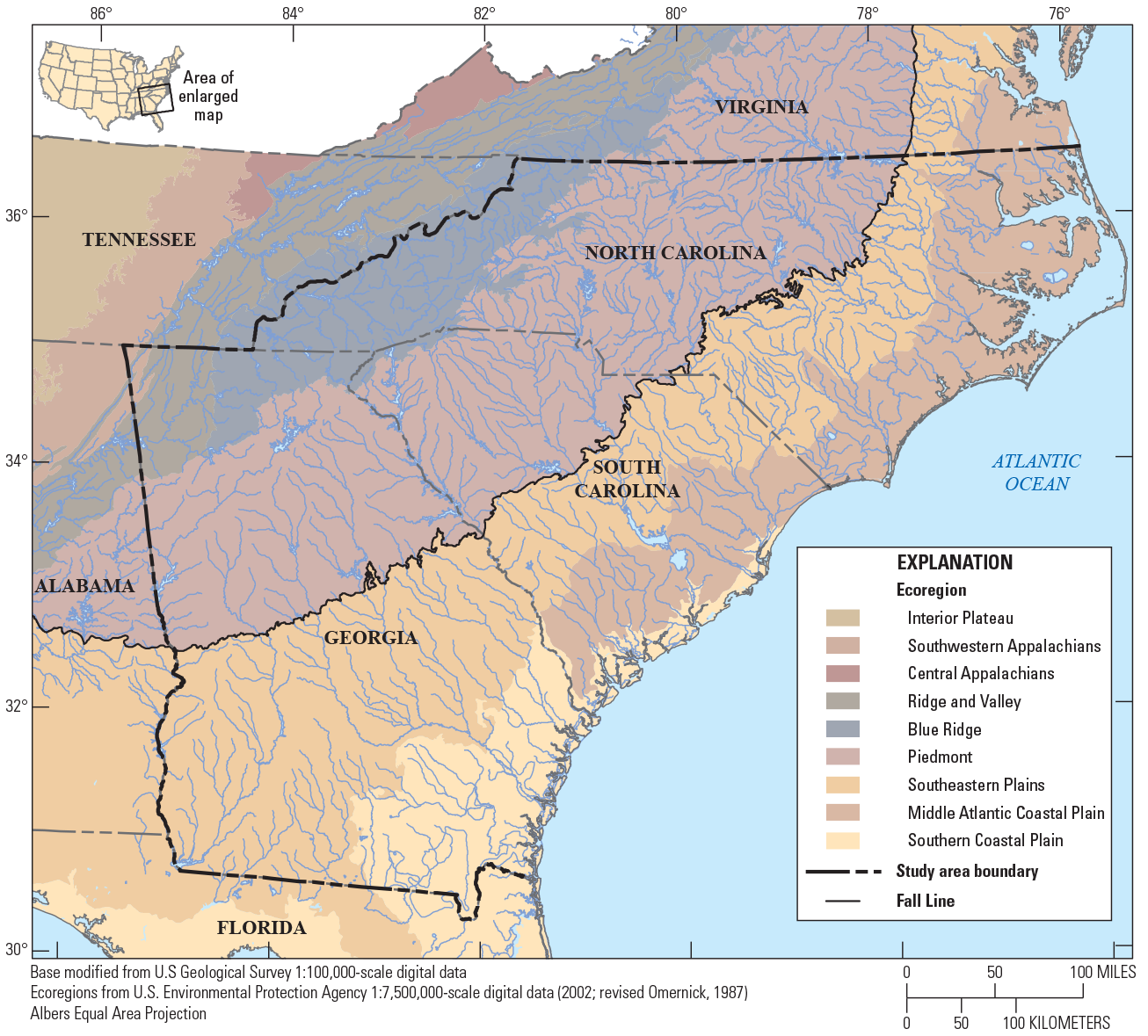
Map showing study area and ecoregions in Georgia, South Carolina, North Carolina, and surrounding States.
The Southwestern Appalachians ecoregion is composed of open, low mountains. The eastern boundary of this ecoregion, along the more abrupt escarpment where it meets the Ridge and Valley ecoregion, is relatively smooth and only slightly notched by small, eastward-flowing streams (Griffith and others, 2001, 2002). The Ridge and Valley ecoregion is composed of roughly parallel ridges and valleys with a variety of widths, heights, and geologic materials. Springs and caves are relatively numerous (as compared to other ecoregions), and present-day forests cover about 50 percent of the ecoregion. The Blue Ridge ecoregion varies from narrow ridges to hilly plateaus to more mountainous areas. The mostly forested slopes; high-gradient, cool, clear streams; and rugged terrain overlie primarily metamorphic rocks, with minor areas of igneous and sedimentary deposits. The Piedmont ecoregion is composed of a transitional area between the mostly mountainous ecoregions of the Appalachians to the northwest and the relatively flat Coastal Plain to the southeast. The Piedmont ecoregion is a complex mosaic of metamorphic and igneous rocks of Precambrian and Paleozoic age, with moderately dissected irregular plains and some hills. The soils tend to be finer textured than in the Coastal Plain ecoregions to the south. Once largely cultivated, much of this ecoregion has reverted to pine and hardwood forests, with increasing conversion to urban and suburban land cover (Omernik, 1987).
The Southeastern Plains ecoregion is composed of irregular plains with a mixture of cropland, pasture, woodland, and forest (Griffith and others, 2001, 2002). The sand, silt, and clay geology of this ecoregion contrasts with the older rocks of the Piedmont ecoregion. Altitudes and relief are greater than in the Southern Coastal Plain ecoregion but generally are less than in much of the Piedmont ecoregion. Streams have relatively low gradient (as compared to the Piedmont ecoregion) with sandy bottoms. The Southern Coastal Plain ecoregion consists of mostly flat plains, but it is a heterogeneous ecoregion containing barrier islands, coastal lagoons, marshes, and swampy lowlands along the Gulf and Atlantic coasts. This ecoregion is lower in altitude with less relief and wetter soils than the Southeastern Plains ecoregion. The Middle Atlantic Coastal Plain ecoregion consists of low-altitude flat plains, with many swamps, marshes, and estuaries. Unconsolidated sediments underlie the low terraces, marshes, dunes, barrier islands, and beaches. Poorly drained soils are common, and the ecoregion has a mix of coarse and finer textured soils compared to the mostly coarse soils in the majority of the Southeastern Plains ecoregion. The Middle Atlantic Coastal Plain ecoregion typically is lower, flatter, and more poorly drained than the Southern Coastal Plain ecoregion (Omernik, 1987).
The average annual precipitation for the study area generally ranges from 40 to 60 inches per year (in/yr). The southern portion of the Blue Ridge ecoregion receives up to or more than 80 in/yr of precipitation (PRISM Climate Group, 2015a). Precipitation in the study area is associated with the movement of warm and cold fronts from November through April and isolated summer thunderstorms from May through October. Occasionally, tropical storms or hurricanes that enter along the Atlantic and Gulf coasts produce unusually heavy amounts of rainfall. The mean annual air temperature in the study area ranges from 54 degrees Fahrenheit (°F) in northern North Carolina to 68 °F in southern Georgia, with variations as low as 46 °F in some of the higher Blue Ridge altitudes in western North Carolina (PRISM Climate Group, 2015b).
Data Compilation
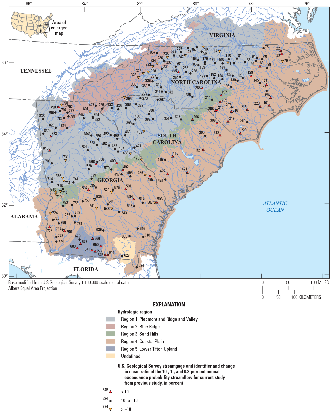
The data used in the regionalization of flood characteristics consists of peak-flow data from streamgages and their respective basin characteristics as explanatory variables in the regression. Peak-flow records through water year 2017 from streamgages in Georgia, South Carolina, and North Carolina and adjacent parts of Alabama, Florida, Tennessee, and Virginia with 10 or more years of annual peak-flow data were considered for use in this study. Many streamgages recorded flood magnitudes of historic levels during water year 2018 (outside the study period). Because of the importance of considering large floods in frequency analysis, the 2018 peaks from select streamgages were incorporated in this study. Peak-flow records were obtained from the USGS National Water Information System (NWIS; U.S. Geological Survey, 2019) and reviewed for quality assurance and quality control (QA/QC) by using the PFReports computer program as detailed by Ryberg and others (2017). The QA/QC analysis resulted in the selection of 965 streamgages that were considered for use in this study (fig. 2; table 1 from Kolb and others, 2023).
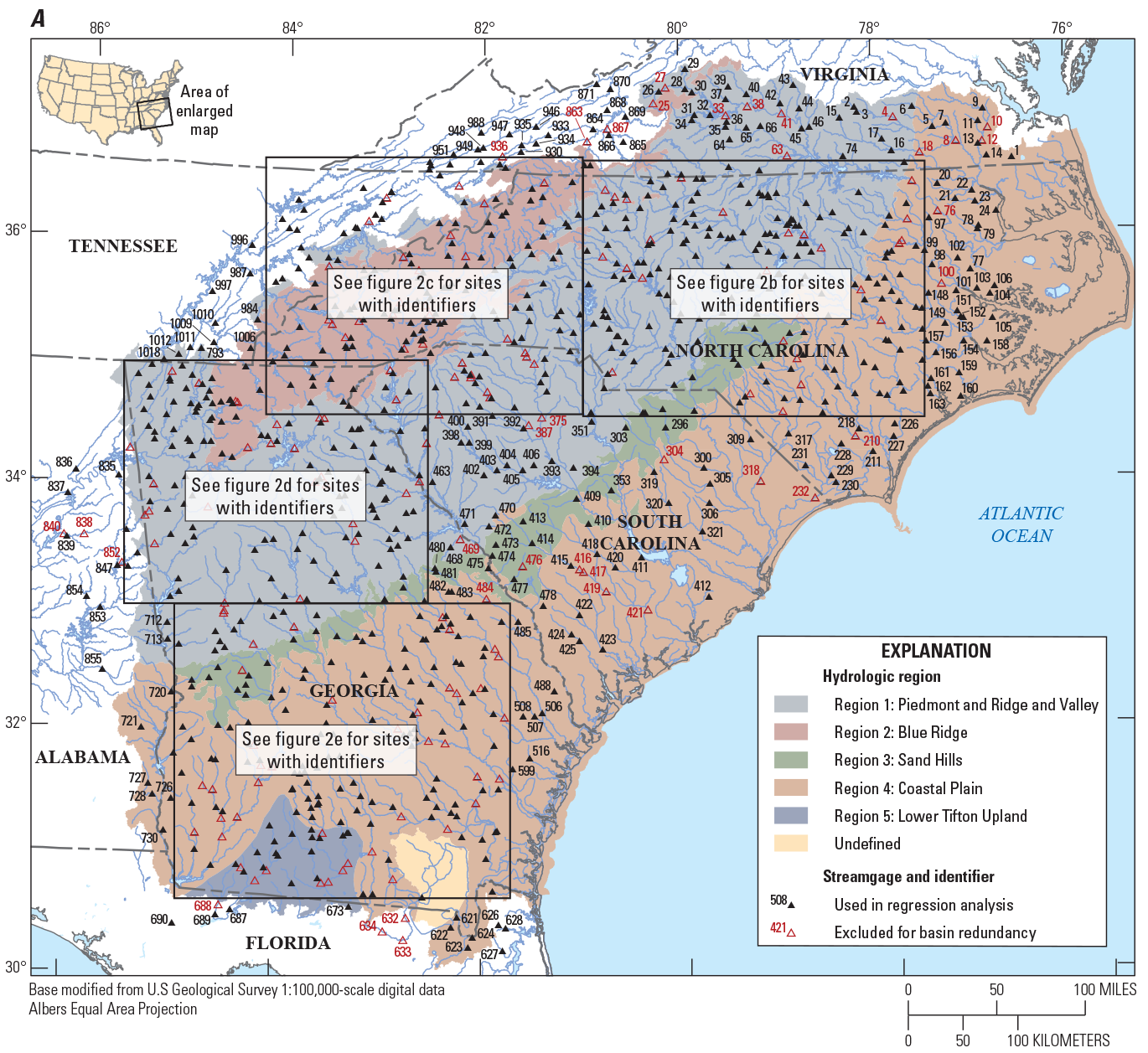
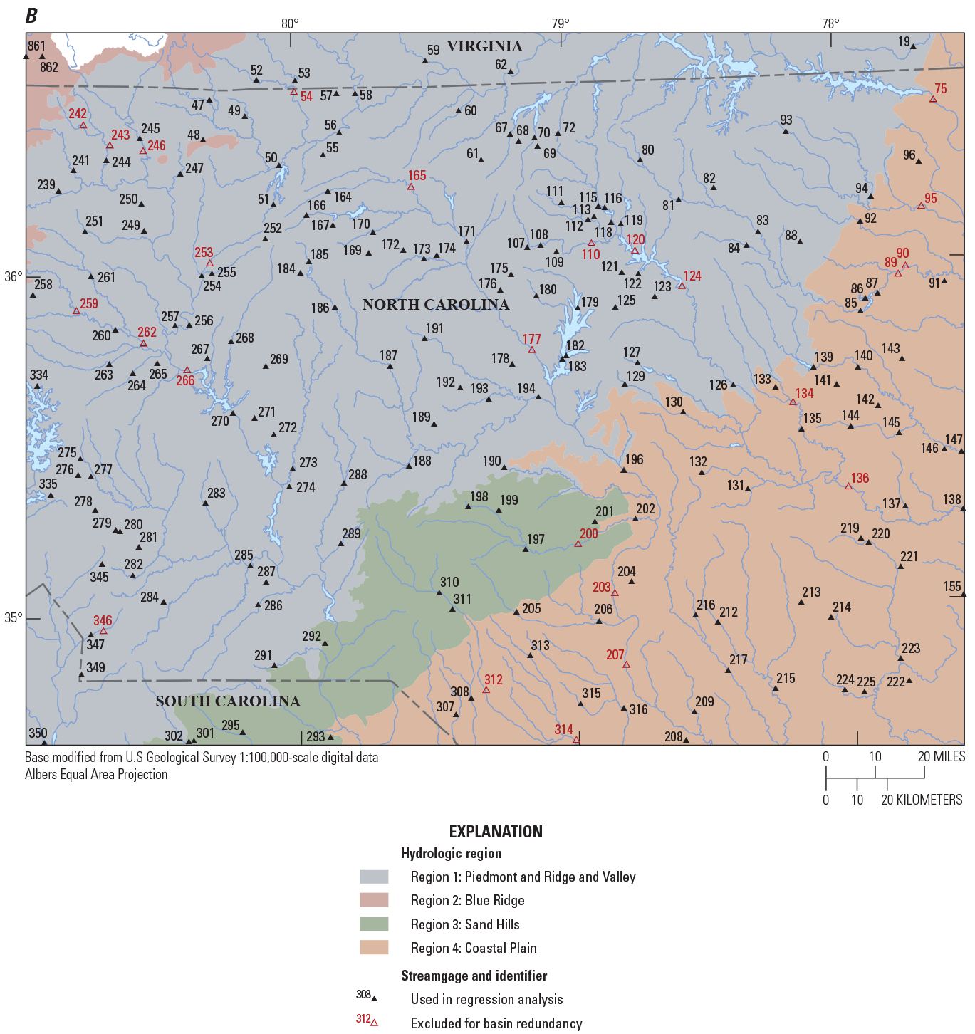
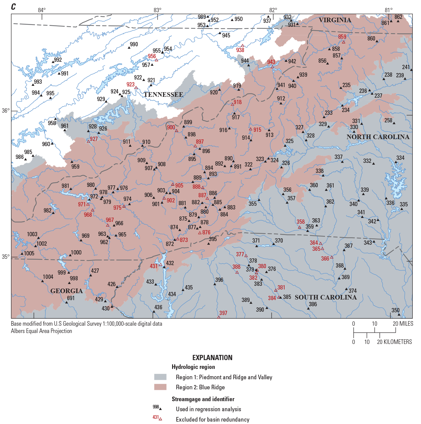
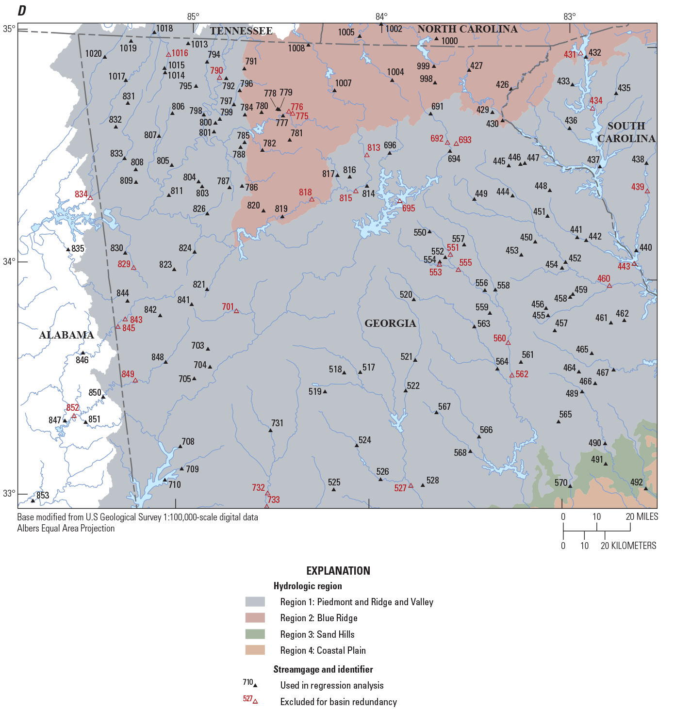
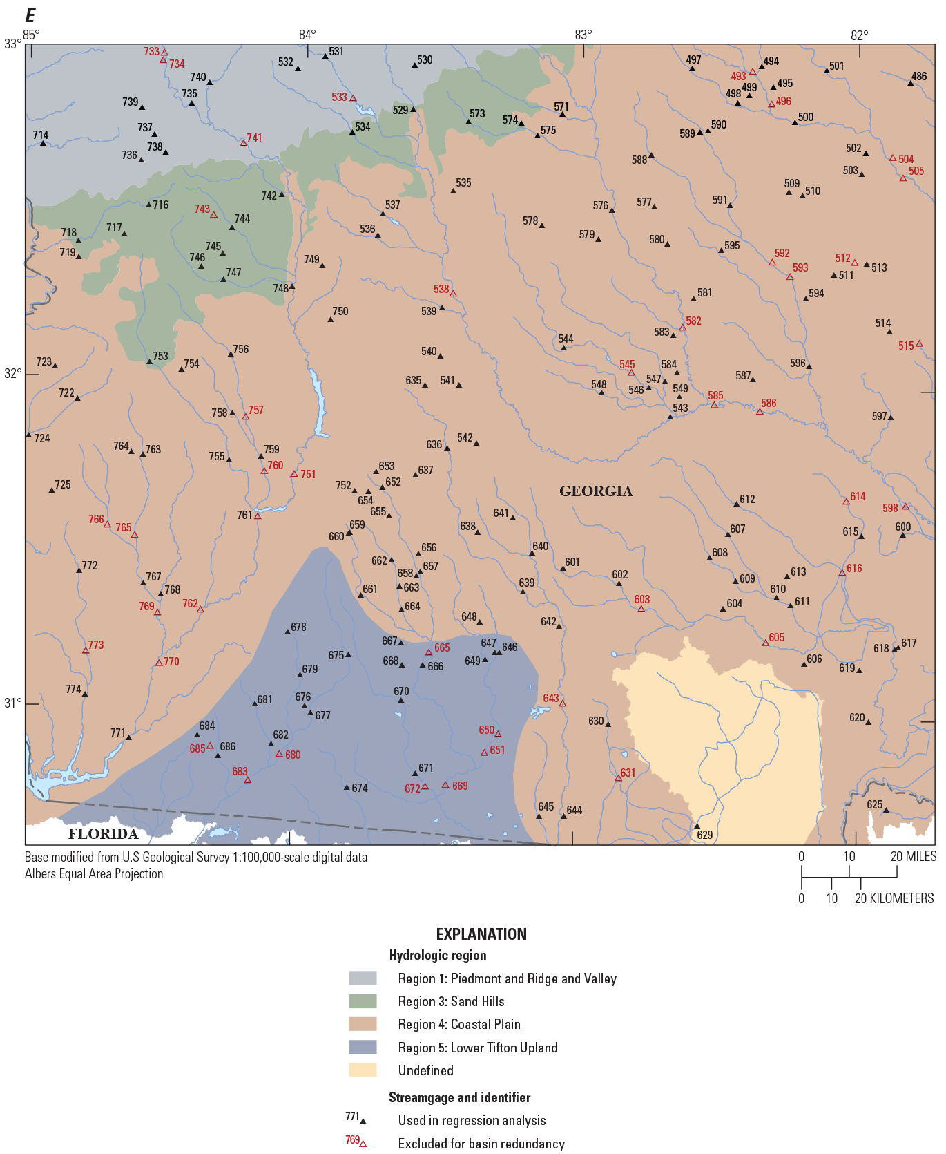
Maps showing hydrologic regions and locations of U.S. Geological Survey streamgages with 10 or more years of record that were considered for use in the regional regression analysis for rural streams in Georgia, South Carolina, North Carolina, and surrounding States.
Streamgages were used in the analysis only if 10 or more years of annual peak-flow data were available, and if peak flows at the streamgages were not affected substantially by dam regulation, flood-retarding reservoirs, tides, or urbanization. The peak-flow record for rural streamgages that met the criteria above then were compiled and reviewed using the PFReports computer program as detailed by Ryberg and others (2017). As discussed further in the “Statistical Analysis of Trends in Annual Peak Flows” section, the Kendall’s tau was chosen to assess the significance of flow-frequency trends for each streamgage (Helsel and others, 2020).
Physical and Climatic Basin Characteristics
Basin characteristics were selected for use as potential explanatory variables in the regression analyses based on the well-established theoretical and empirical relationships between these parameters and runoff characteristics and the ability to measure the basin characteristics in a geographic information system (GIS). For each of the 965 streamgages considered, 26 basin characteristics (such as drainage area, mean basin elevation, mean annual precipitation) were determined and considered as potential explanatory variables in the regression analyses (table 2 from Kolb and others, 2023).
Drainage-basin boundaries for this study were generated using the USGS StreamStats application (Ries and others, 2017) and used to determine the 26 basin characteristics. The underlying altitude data in the StreamStats program were generated using two different GIS data sources. In Georgia, StreamStats data were generated from National Elevation Dataset digital elevation models (DEMs) with 10‑meter (m) resolution (U.S. Geological Survey, 2014). In North Carolina, StreamStats data were generated from National Elevation Dataset DEMs with 30‑foot (ft) resolution (U.S. Geological Survey, 2014). The South Carolina StreamStats data were generated using 30‑ft resolution DEMs (Kolb and others, 2018) derived from light detection and ranging (lidar) data from the South Carolina Department of Natural Resources (2015). Boundary delineations were compared with NWIS drainage areas for QA/QC, as this was the first flood‑frequency study completed since the implementation of StreamStats for the South Atlantic Water Science Center (SAWSC). In the case of erroneous delineations (such as a missed culvert), the boundaries and drainage area values were improved using aerial imagery and DEMs. More information about the StreamStats applications in South Carolina, Georgia, and North Carolina is available in Feaster, Clark, and Kolb (2018), Gotvald and Musser (2015), and Weaver and others (2012), respectively.
Drainage-basin boundaries generated from StreamStats were compared to previously published drainage areas for the streamgages as a means of QA/QC. For most streamgages, the drainage areas agreed closely but for various streamgages, the drainage areas differed by more than 2 percent. In most cases where the difference exceeded this threshold (greater than 2 percent), the published drainage areas were determined manually from older topographic maps with 10‑ft contour intervals. Boundaries generated using StreamStats were considered more accurate than manual delineations. The streamgages with drainage area differences greater than 2 percent were revised to the StreamStats generated drainage-basin boundaries (U.S. Geological Survey, 2012).
Statistical Analysis of Trends in Annual Peak Flows
In this study, Kendall’s tau nonparametric test (Kendall, 1938) was used to determine statistical significance of monotonic trends in annual peak flow with time (Helsel and others, 2020). A trend was considered statistically significant for a probability value (p-value) less than or equal to 0.05. Kendall’s tau measures the degree of correspondence between two variables (for example, x and y). For this analysis, the x and y variables are water year and annual peak flow, respectively. A concordant pair results when both x and y variables increase or decrease; a discordant pair results when x increases and y decreases or x decreases and y increases. The number of concordant pairs and the number of discordant pairs were tallied for each streamgage considered here and the Kendall’s tau value (τ) was computed using the following equation:
whereThe null hypothesis for this test is that there is no monotonic trend between the peak flows and time and the p-value of 0.05 indicates there is less than a 5‑percent chance of obtaining the sample result if the null hypothesis were true.
If the data indicate perfect positive correlation, then τ = 1; if there is perfect negative correlation, then τ = −1; and if there is no correlation between the pairs, then τ = 0. Therefore, a positive τ value is associated with an upward trend and a negative τ value is associated with a downward trend (Norton and others, 2014).
For hydrologic time-series data, Kendall’s tau test is best suited for analysis of long-term datasets. Although it can be applied to short time series, Kendall’s tau test may not provide information that is of practical importance, and care is needed to avoid misinterpreting the results. Tests applied to short time series may (1) fail to detect a statistically significant trend even though a large increase or decrease in flow has been measured, or (2) detect a statistically significant trend even though the trend is of no practical importance (Oki, 2004). Thus, long-term streamgaging data are better suited for trend assessments. The USGS typically considers 30 years of streamflow record as an appropriate threshold to designate long-term streamgages (U.S. Geological Survey, 2009).
Of the 965 streamgages that were considered for use in the regional regression analysis, a Kendall’s tau test was performed using annual peak flows for streamgages with 30 or more years of record. The results of the trend analyses of the annual peak flows are shown in table 1 from Kolb and others (2023). Of the streamgages considered in table 1 from Kolb and others (2023), 495 contain 30 or more years of systematic streamflow peaks and are considered long-term streamgages with 332 of those long-term streamgages operating in 2017 (stations with combined records were not included in the trend analysis). Of the 332 long-term streamgages, 276 streamgages (83 percent) indicated no statistically significant trend (p-value >0.05) in annual peak flows, 45 streamgages (14 percent) indicated a statistically significant downward trend, and 11 streamgages (3 percent) indicated a statistically significant upward trend (fig. 3A).
For comparison of trends as record length increases (fig. 3A–D), an assessment of significant trends for the current long-term streamgages was done for four groups of stations: (1) from 30 to 49 years, (2) from 50 to 69 years, (3) from 70 to 89 years, and (4) 90 or more years of annual peak flows (fig. 4). As the data-record length increased, the percentage of streamgages with significant upward and downward trends remained relatively consistent. There are many streamgages with significant downward trends in the middle portion of eastern Georgia, as well as western and central South Carolina (fig. 3). The streamgages in these areas recorded large floods in the early part of the 20th century and multiple drought periods in the early part of the 21st century, which resulted in downward trends (see fig. 5 for an example of this result at USGS streamgage 02191300, site 452 on fig. 2). Significant upward trends also result in a small portion of southern Georgia and northern Florida (fig. 3). The streamgages in those areas recorded more frequent larger floods from water years 1985 to 2017, which resulted in the upward trends (see fig. 6 for an example of this result at USGS streamgage 02329000, site 687 on fig. 2). A comprehensive analysis of the causes of the trends in the annual peak flows is outside the scope of this report. Because of the lack of strong and consistent statistical evidence of significant long-term regional peak-flow trends throughout the study area, the traditional assumption of stationarity is used for this study with no adjustment for either upward or downward trends.
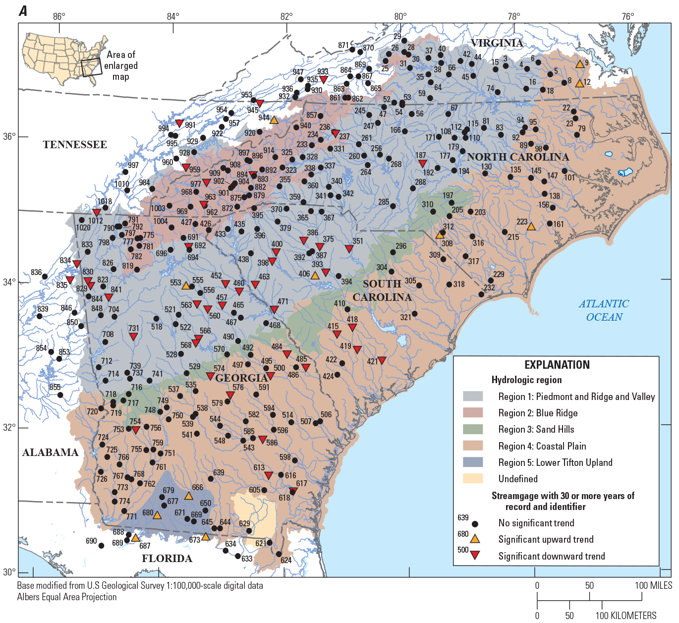
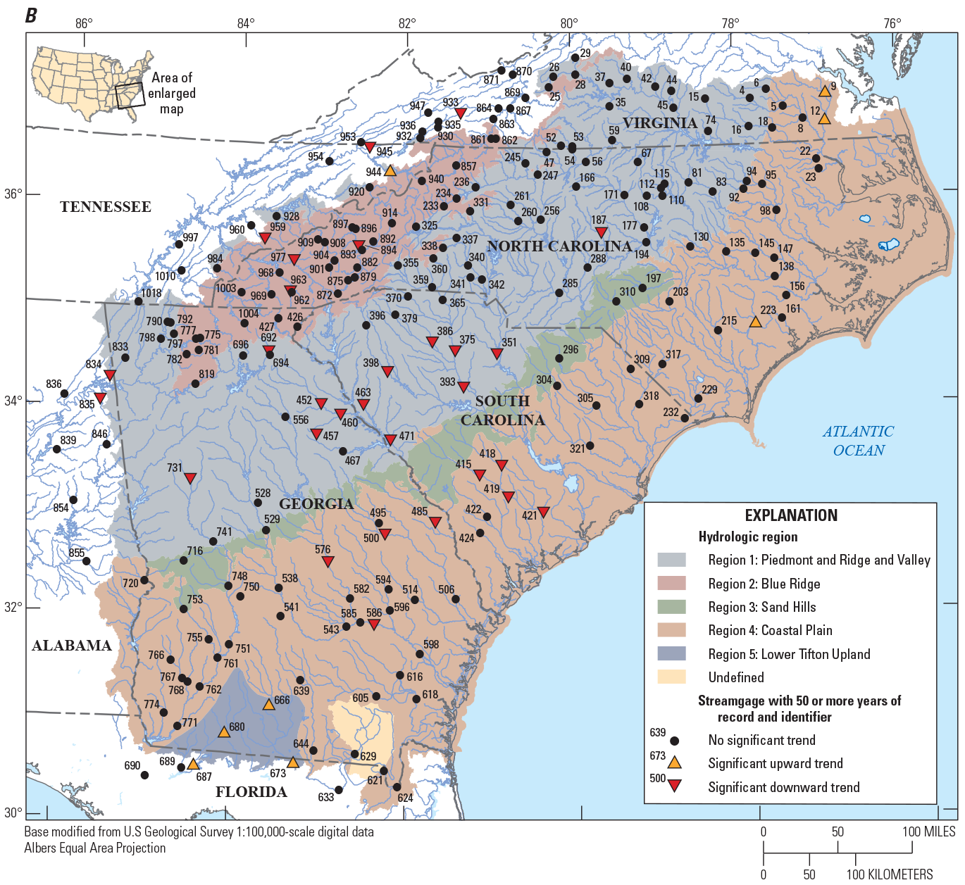

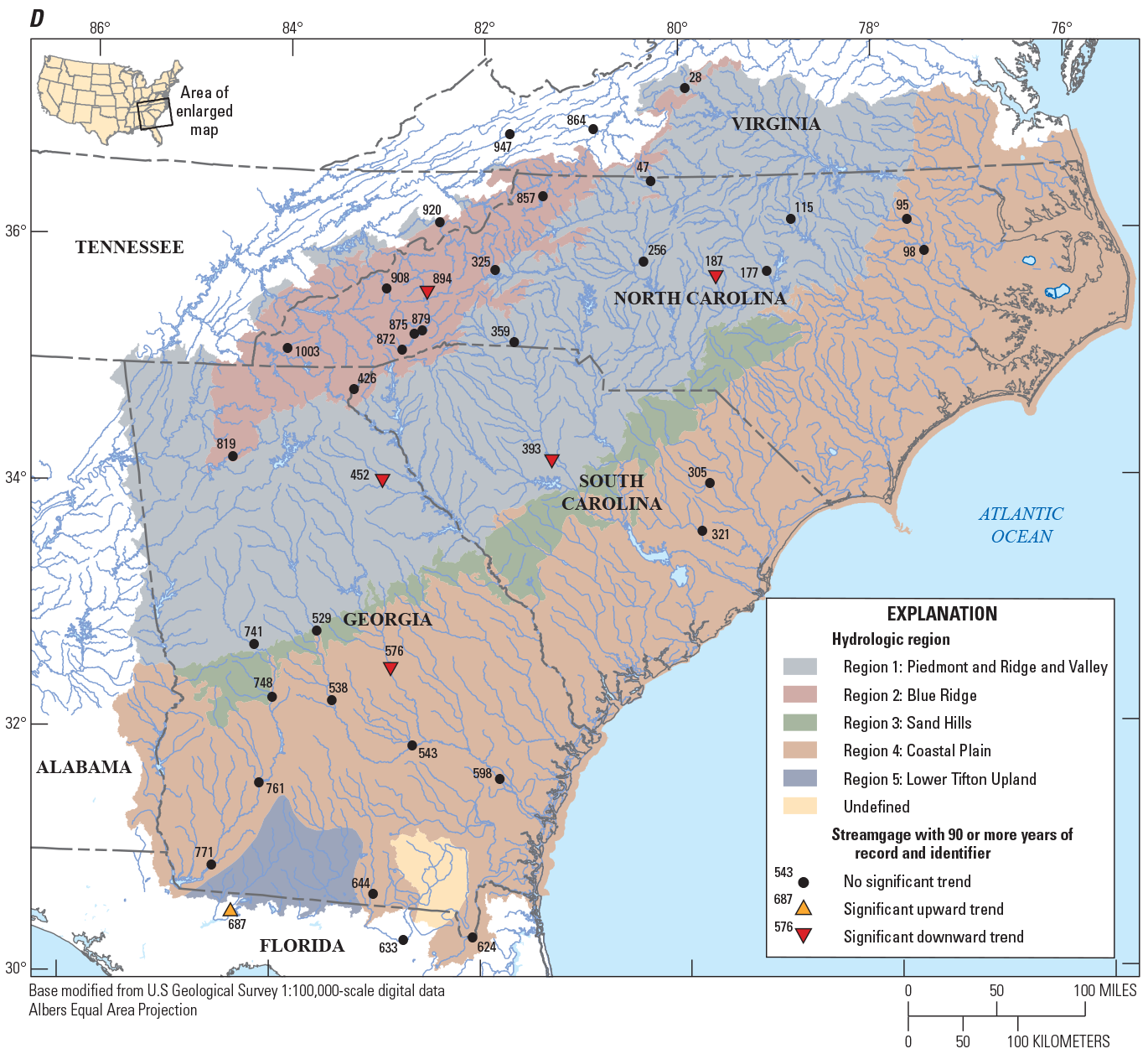
Maps showing the direction of significant trends in the annual peak flow of 332 U.S. Geological Survey streamgages with current (2017) data with (A) 30 or more years of annual peak flows, (B) 50 or more years of annual peak flows, (C) 70 or more years of annual peak flows and (D) 90 or more years of annual peak flows, in Georgia, South Carolina, North Carolina, and surrounding States.
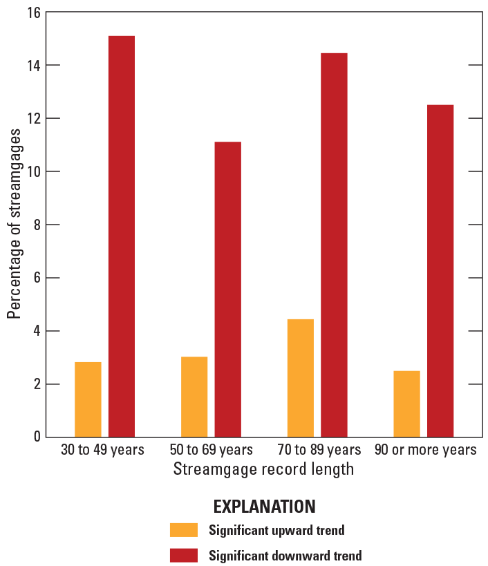
Graph showing percentage of streamgages with significant upward and downward trends for the U.S. Geological Survey streamgages in Georgia, South Carolina, North Carolina, and surrounding States, with current (2017) peak-flow data and 30 to 49 years, 50 to 69 years, 70 to 89 years, and 90 or more years of annual peak flows.
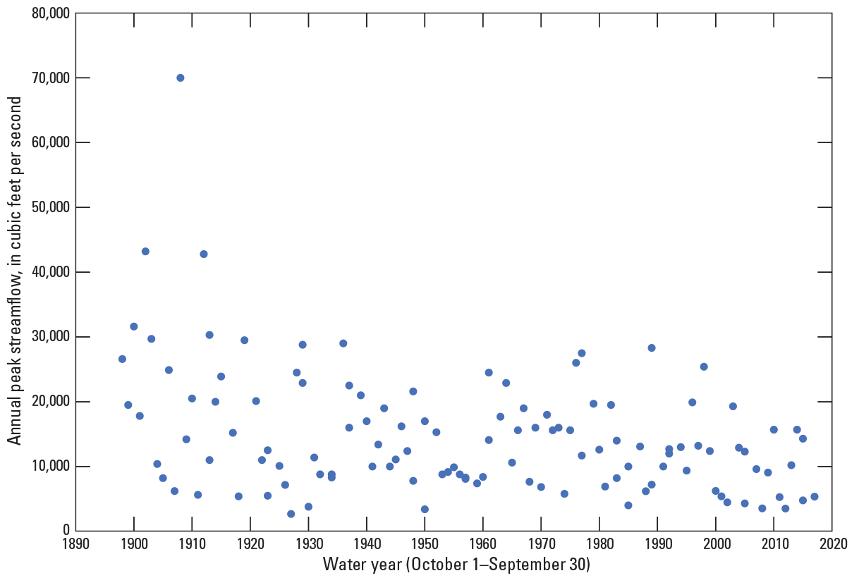
Graph showing annual peak flows for water years 1890 through 2020 for U.S. Geological Survey streamgage 02191300, Broad River above Carlton, Georgia (site 452 on fig. 2).
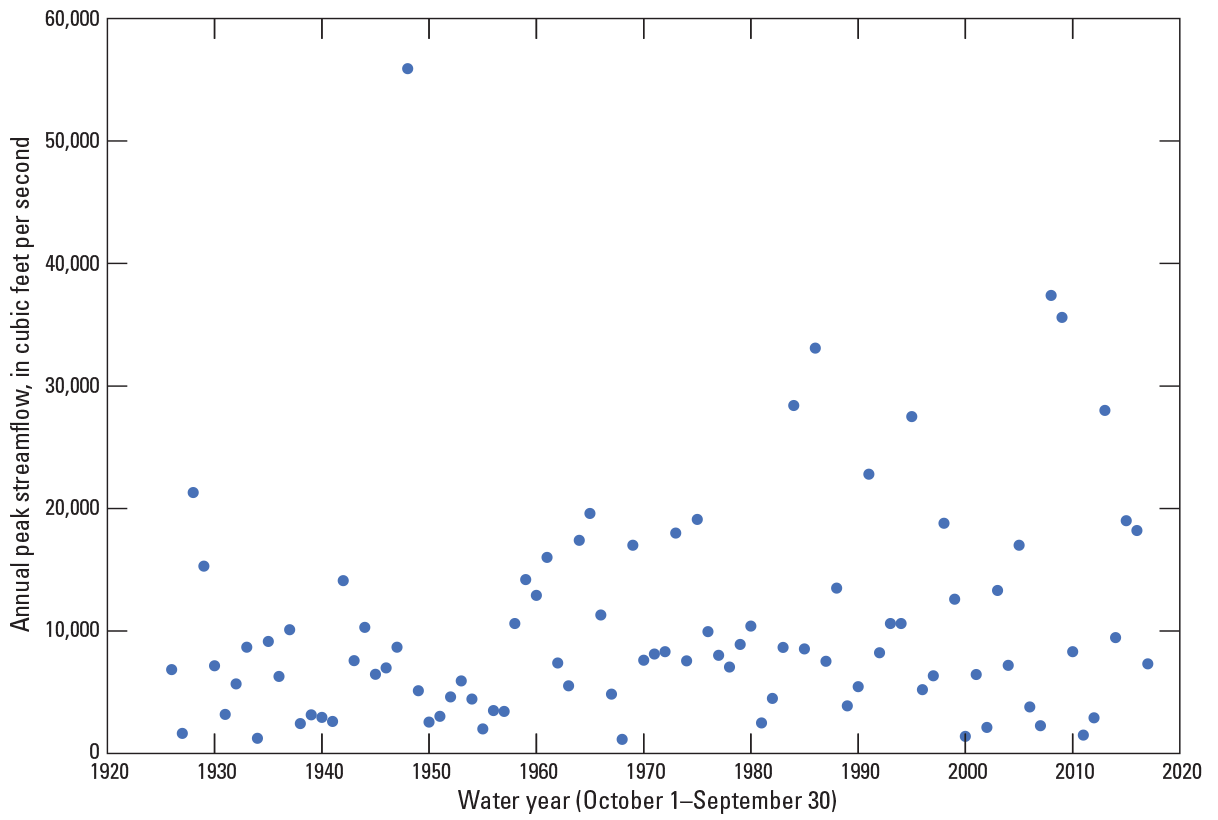
Graph showing annual peak flows for water years 1920 through 2020 for U.S. Geological Survey streamgage 02329000, Ochlockonee River near Havana, Florida (site 687 on fig. 2).
Estimation of Flood Magnitude and Frequency at Streamgages
Flood magnitude and frequency analyses were completed using the methodology described in the current version of the national guidelines for flood‑frequency analysis, Bulletin 17C (England and others, 2019), which was released shortly after the start of this study. Bulletin 17C retains the basic statistical framework of the superseded Bulletin 17B guidelines (Interagency Advisory Committee on Water Data, 1982; Koltun, 2019).
Annual peak-flow data used in flood‑frequency analyses are categorized as either systematic data or historic data. The systematic data are measured as part of the operation of a streamgage. The historic data can take on various forms including (1) observations of large flows that resulted outside of the period of systematic record, (2) knowledge that one or more floods within the period of systematic record are the largest in a longer period, and (3) knowledge that flood magnitudes did not exceed a given value during a period outside of the period of systematic record. The period of systematic record, together with the intervening years between the systematic and historic peak flows, define the historical period of the streamgage.
The Bulletin 17C methodology computes the magnitude of floods for selected AEPs at a streamgage based on statistical properties (or moments) associated with its annual peak-flow record. The Bulletin 17C methodology continues to prescribe the log-Pearson type III (LPIII) distribution with log transformation of the annual peak flows (Interagency Advisory Committee on Water Data, 1982). The LPIII distribution is a three-parameter distribution that requires estimates of the mean, the standard deviation, and the skew coefficient of logarithms of annual peak flow at a streamgage. By determining the mean, standard deviation, and skew of the log-transformed annual peak-flow data, the following equation may be used to compute the magnitude of observed flood flow for a desired AEP and given as
whereQp
is the flood magnitude at a selected percent AEP,
X̅
is the mean of the logarithms of the annual peak flows,
Kp
is a factor based on the skew coefficient and the selected percent AEP, and
S
is the standard deviation of the logarithms of the annual peak flows.
Although maintaining the moments-based approach of the Bulletin 17B procedures, the method outlined in Bulletin 17C introduces the expected moments algorithm (EMA) (Cohn and others, 1997; Roland and Stuckey, 2019), an improved method-of-moments approach for fitting the LPIII distribution to the flood peaks that was used for this study. Application of this new method can accommodate interval estimates of peak flow, censored estimates of peak flow, and multiple thresholds of observation. Bulletin 17C also includes a generalization of the Grubbs Beck low-outlier test (called the multiple Grubbs Beck test [MGBT; Grubbs and Beck, 1972; Cohn and others, 2013]) that permits identification of multiple potentially influential low floods (PILFs). Additionally, new methods for estimating regional skew and uncertainty (Veilleux and others, 2011) are provided in Bulletin 17C.
Flow Intervals and Perception Thresholds
The EMA method outlined in Bulletin 17C and briefly described above accommodates interval peak-flow data, which simplifies analysis of datasets containing censored observations, historic data, low outliers, and uncertain data points, whereas also providing enhanced confidence intervals for the estimated streamflows (Veilleux and others, 2014). The EMA methodology has been incorporated into the USGS peak-flow frequency analysis program, PeakFQ version 7.4 (Flynn and others, 2006; Veilleux and others, 2014; U.S. Geological Survey, 2022), and was used to compute the AEP flows for streamgages in this study. Within the EMA framework, flow intervals and perception thresholds are defined for each year in the annual peak-flow record of any streamgage. The published guidelines (Bulletin 17C) for determining flood flow frequency include many examples of flow intervals and perception thresholds as inputs to EMA to illustrate applications of the recommended techniques.
Flow intervals (defined with a lower and upper bound based on observations, written records, or physical evidence) are used to describe the peak-flow value. For most peak flows during the systematic period of record, the default lower and upper bounds of the streamflow interval both equal the observed peak flow, and for most years when no information has been recorded, the default lower and upper bounds are zero and infinity, respectively. If there is uncertainty in a peak-flow value for a given water year, the lower and upper bounds of the streamflow interval may be set to a range of probable streamflows.
Perception thresholds (lower and upper) identify the range of potentially measurable flood flows where the flow magnitude would have been measured had they occurred (England and others, 2019). Whereas a flow interval applies to a specific single occurrence of peak flow that results in a given water year, the range of streamflow specified in a perception interval is applicable over a given time range (usually a period of years). Generally, for annual peak flows recorded during the systematic period of record of a streamgage, the default perception thresholds range from zero to infinity. If the peak flow is unknown because the streamgage was discontinued or ceased operation, the perception thresholds are both set to infinity.
At some streamgages, flows can be determined only when water in the stream reaches a certain minimum measurable level. For example, it is possible that in some years, the water will not reach that minimum level or the bottom of a crest-stage gage (CSG); consequently, the lower perception threshold is the flow associated with the minimum measurable water level. For this study, years with measurable streamflow were assigned the default perception thresholds of zero to infinity. Alternatively, years when water did not reach the minimum level of measurement were generally assigned a lower perception threshold of either (1) the flow associated with the minimum measurable water level, or if that was not known, (2) one-half of the lowest flow associated with the systematic annual peak-flow record; upper thresholds were set to infinity. In some instances, historic peaks are documented as part of an annual peak-flow record; that is, a peak flow associated with a major flood event outside of the systematic period of record for the streamgage. For the ungaged years between the historic and systematic peaks, the lower perception threshold is typically set to a value the analyst determines would have been measured during minimum flow conditions, and the upper threshold is set to infinity. The flow interval and perception thresholds that were incorporated into the EMA analysis for each streamgage included in this study are provided in the associated data release (Kolb and others, 2023).
Occasionally, a streamgage site had a documented historic peak-gage height (record of flood height outside of the systematic period of record) with no associated peak flow. In these instances, a peak flow (or peak-flow range) was estimated based on a comparison to other peak-gage height and associated flow values at the site of interest.
In some instances, documented peak flows occurred outside of the systematic period of record, and were categorized as an opportunistic peak flow. Opportunistic peaks were measured based on factors other than the exceedance of a perception threshold and, thus, were not treated as historic peaks. Furthermore, these flows are not truly random as their sampling properties are unknown. Consequently, opportunistic peaks were not included in the flood‑frequency analyses because of the potential to bias the sample streamflow records.
Flow intervals used in the analyses of unregulated streamgage records are reported in table 5 from Kolb and others (2023). Perception thresholds used in the analyses of unregulated and regulated streamgage records are reported in tables 6 and 7 from Kolb and others (2023), respectively. Inputs to PeakFQ, which include all flow intervals and perceptions thresholds used in this study, are presented in Kolb and others (2023). The report files from the PeakFQ analyses also are available in Kolb and others (2023).
Potentially Influential Low Flows
Low-magnitude peaks that depart significantly from the sample of annual peak flows for a streamgage can result in a poor fit of the frequency curve at lower AEPs. When evaluating the sample of annual peak flows, attention must be given to annual peaks that are considered outliers. Referred to as potentially influential low flows (PILFs), these peak flows may appreciably affect the upper end of the peak-flow distribution, which tends to be most important for a flood‑frequency analysis.
The multiple Grubbs Beck test (MGBT; Cohn and others, 2013) is an option in the PeakFQ software to identify and censor PILFs. Censoring the PILFs typically results in improved agreement between the high end (where AEPs are small, such as the 0.2‑percent AEP) of the observed frequency distribution and the high end of the estimated frequency distribution. In some instances, censoring the PILFs may degrade the fit at the low end (where AEPs are large, such as the 50‑percent AEP) of the frequency distribution. As recommended in Bulletin 17C guidelines, for instances when PILFs were identified by means of the MGBT, a careful analysis of the PILFs was conducted by applying local knowledge of the watershed and hydrologic considerations. This analysis was used to determine whether the use of the MGBT was appropriate for the identification of PILFs.
Regional Skew Coefficient
The regional skew coefficient is associated with a defined region and is derived from an analysis of skew coefficients for streamgages with longer annual peak-flow records within the defined region. The skew coefficient measures the asymmetry of the probability distribution of a set of annual peak flows. The skew coefficient is zero when the mean of the annual series equals the median and the mode; positive when the mean exceeds the median, which in turn exceeds the mode; and negative when the mean is less than the median, which, in turn, is less than the mode (fig. 7). The skew coefficient is strongly affected by the presence of outliers. Large positive skews typically are the result of high outliers, and large negative skews typically are the result of low outliers. The streamgage skew coefficient, which is calculated by using the annual peak-flow record for a streamgage, is sensitive to extreme hydrologic events; therefore, the streamgage skew coefficient for short records may not provide an accurate estimate of the true skew coefficient.
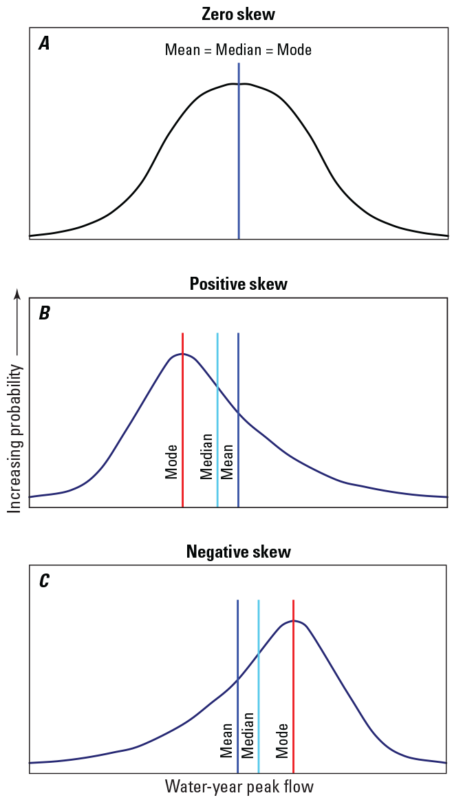
Graphs showing examples of distributions with (A) zero skew, (B) positive skew, and (C) negative skew (modified from Feaster and Tasker, 2002).
Bulletin 17C recommends the skew coefficient used in defining the probability distribution be a weighted average of the streamgage skew coefficient and a regional skew coefficient that reflects regional and long-term (decadal) conditions (England and others, 2019). As part of this study, the regional skew was updated using Bayesian WLS/Bayesian GLS methodology, and the procedures and results are presented in appendix 1. Flood‑frequency estimates for streamgages with unregulated flow were computed using a weighted average of the streamgage skew and the regional skew. The following equation shows how the weighted skew coefficient for a given site is computed:
whereComparison of Selected Flood‑frequency Estimates with the Previous Estimates
Flood‑frequency statistics are dynamic values being strongly influenced by length of record and hydrologic conditions captured in those records. A spatial analysis of the changes in the weighted flood‑frequency estimates for 199 selected streamgages in Georgia, South Carolina, and North Carolina is included in this study. These streamgages have at least 30 years of systematic record with at least 8 additional years of peak-flow record since the previous rural flood‑frequency study (Feaster and others, 2009; Gotvald and others, 2009; Weaver and others, 2009). The analysis was performed to assess the effects of additional peak-flow data on the weighted flood‑frequency estimates, which is done using the estimate at a streamgage with the regional regression estimate for the same location. The procedure for weighting flood‑frequency estimates is detailed later in this report. The analysis comparing the flood‑frequency from this study with those from the previous study was performed using the weighted flood‑frequency estimates for the 10‑, 1‑, and 0.2‑percent AEP streamflows.
A ratio of the current weighted AEP streamflow divided by the weighted AEP streamflow from the previous rural flood‑frequency study was computed for each of three AEP flows (10‑, 1‑, and 0.2‑percent), and then the mean of the three ratios was determined. The means of the three ratios were divided into three categories: greater than 1.1 (10 percent or more increase in the weighted AEP streamflows), less than 0.9 (10 percent or more decrease in the weighted AEP streamflows), and between 1.1 and 0.9 (minimal change in the weighted AEP streamflows). The results of this analysis are presented in figure 8.
For 120 of the 199 streamgages considered in this analysis (60 percent), the mean ratio of the 10‑, 1‑, and 0.2‑percent AEP streamflows from this and the previous rural flood‑frequency study was within 10 percent. At 44 streamgages (22 percent), the mean ratio increased by over 10 percent, and at 35 streamgages (18 percent), the mean ratio decreased by over 10 percent. Many of the streamgages where the selected AEP streamflows mean ratios decreased were in hydrologic regions 1 and 2. Many of the streamgages where the mean AEP streamflow ratios increased were in hydrologic regions 4 and 5 (fig. 8). For the streamgages in hydrologic region 3, the mean ratios of the three AEP streamflows have increased or exhibit minimal changes. It’s worth noting that hydrologic regions 3, 4, and 5 are all located in the Coastal Plain, an area that has experienced several historical flood events since the last flood‑frequency study.
Map showing percentage change in the mean ratio of the 10‑, 1‑, and 0.2‑percent annual exceedance probability streamflows for selected streamgages from the current study to a previous rural flood‑frequency study (Feaster and others, 2009; Gotvald and others, 2009; Weaver and others, 2009) for five hydrologic regions in Georgia, South Carolina, North Carolina, and surrounding States.
Streamgages Affected by Regulation
In this study, regulation of peak flows refers to natural streamflows being impounded by dams. Peak flows can also be affected by urbanization, channelization, and mining, which are generally considered to be an alteration or diversion of streamflow as compared to regulation of streamflow resulting from an impoundment in the basin. For this report, the initial determination of whether peak flows were affected by regulation was based primarily on peak-flow qualifier codes in the USGS peak-flow database (U.S. Geological Survey, 2019). Streamgage descriptions and other supporting documentation contained in the USGS Site Information Management System, which is an internal data management program, were also reviewed for supporting information. Peak flows affected by dam failure were not used in any of the flood‑frequency analyses.
Bulletin 17C notes that one area of future work needed is in developing national guidance for computing flood‑frequency estimates on regulated streams (England and others, 2019). The Subcommittee on Hydrology, Hydrologic Frequency Analysis Work Group suggested that Bulletin 17B techniques could be used for regulated watersheds if the logarithms of the regulated peak flows were determined to be relatively consistent with an LPIII distribution (Advisory Committee on Water Information, 2021). Another important factor that should be considered for a regulated flood‑frequency analysis is whether or not the effects of regulation were consistent over the period of record. If substantial changes in the regulation patterns are indicated, the most recent period of relatively stable flow patterns should be used in the flood‑frequency analysis. In this report, only regulated streamgages with at least 20 years of peak flows indicating relatively stable flow patterns were included. Flood‑frequency estimates were computed for 72 regulated streamgages with at least 20 years of peak flows through water year 2019 (table 8 from Kolb and others, 2023) (fig. 9). Of the 72 regulated streamgages, 18 had pre-regulated periods of record that also were analyzed as part of this study.
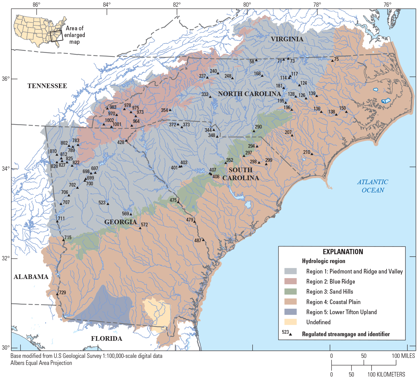
Map showing locations of U.S. Geological Survey streamgages on streams in Georgia, South Carolina, and North Carolina affected by regulated streamflow conditions.
To assess peak-flow patterns at regulated streamgages, the Kendall’s tau test and cumulative plots of the peak flows (single-mass curves) were used. The Kendall’s tau test was applied to assess the strength in the relation between the peak flows over time (Kendall, 1938; Helsel and others, 2020). For regulated streams where regulation patterns might be altered over time, such as below hydropower plants, interpretations of trend analyses are more complicated. Just as with unregulated streams, streamflow in regulated basins can be affected by changes in climate patterns and land cover. However, those effects might be mitigated, enhanced, or even offset by changes in regulation patterns, such as operational procedures or permitting changes. Nonetheless, the Kendall’s tau test can be a useful tool for assessing relative stability of streamflow patterns on a regulated stream. The single-mass curve (SMC) is a basic analytical tool for presenting a plot of a cumulative value over time. The slope of the SMC represents the constant of proportionality between two quantities, which in this case are peak flow and water year (Searcy and Hardison, 1960). A substantial change in the slope of the curve indicates a change in the proportionality constant. In the case of regulated streams, the SMC is another analytical tool to help assess whether regulation patterns have been relatively consistent over the analysis period.
In a study of the relation between hydrologic characteristics and flood peaks within a humid region of New England, an assessment of the degree of regulation was made using various measures of storage and drainage area (Benson, 1962). Benson (1962) determined that a usable storage of less than 103 acre-feet per square mile would generally affect peak flows by less than 10 percent. As such, Benson (1962) used that level of usable storage as a limiting value for assuming that peak flows were not substantially affected by upstream regulation. Usable storage is defined as storage that is normally available for release from a reservoir below the maximum controllable water level and, therefore, excludes dead storage, which is the volume of water in a reservoir below the lowest controllable water level (Martin and Hanson, 1966). In many reservoirs, the dead storage tends to be a small or negligible part of the total storage. For this report, maximum storage, in acre-feet, which is defined as the total storage in a reservoir below the maximum attainable water-surface elevation, including any surcharge storage, was obtained from the U.S. Army Corps of Engineers National Inventory of Dams database (U.S. Army Corps of Engineers, 2020), and along with the drainage area at the streamgages, it was used to compute a maximum storage index, in acre-feet per square mile. The maximum storage index, along with other assessment tools, was used to assess the potential degree of regulation of the basin monitored at the streamgage.
Although flood‑frequency estimates for sites with a regulated flow record were computed by fitting the recorded annual regulated peak flows to the LPIII distribution, the streamgage skew was used rather than the weighted skew. Because regulated peak-flow records are not included in the regional skew analysis, the weighted skew techniques are only applicable to unregulated flood‑frequency estimates.
Georgia
Peak-flow data used to derive flood‑frequency estimates for streamgages in Georgia were obtained from the USGS NWIS database (U.S. Geological Survey, 2019). For certain regulated streamgages in Georgia, valuable flood information observed in the unregulated record were incorporated into the regulated record before the flood‑frequency analysis was performed. Historic floods and major floods from the unregulated period were adjusted (reduction in magnitude) to reflect regulated conditions associated with dams and reservoirs. The adjustments to Savannah River peak flows from pre- to post-regulation are based on previously applied methods described in Sanders and others (1990).
Continuous peak flows were assessed at streamgage 02197000, Savannah River at Augusta, Ga. (site 475 on fig. 9), for water years 1875 through 2019. It also has historic peak flows available for water years 1796, 1840, 1852, 1864, and 1865. Although there are various smaller reservoirs in the basin, the first major reservoir built was the J. Strom Thurmond Reservoir in 1952. Lake Hartwell, which is upstream from Thurmond Reservoir, was completed in 1962. Richard B. Russell Reservoir, which is between Hartwell and Thurmond Reservoirs, was completed in 1986. The reservoir system was built for the purposes of flood control and providing hydroelectricity, but also provides water supply and recreation. The slope of the SMC for the peak flows shows a significant shift about 1952 but has been relatively stable since then. Because Thurmond Reservoir has the largest maximum storage capacity of the reservoirs discussed above and is the furthest downstream reservoir in the system, the other reservoirs that came online after Thurmond did not appreciably alter the peak-flow patterns at streamgage 02197000.
Sanders and others (1990) adjusted the historic, unregulated peak flows measured at streamgage 02197000 to account for regulation conditions present at that time. As previously noted, the SMC analysis indicated that peak-flow patterns have been relatively stable at streamgage 02197000 since about 1952. The historic peak flows for 1796, 1840, 1852, and 1865, along with other major floods in 1888, 1908, 1929, 1930, 1936, and 1940 at streamgage 02197000 were adjusted for regulation and combined with the regulated peaks from 1953 through 2019 at the site to derive the AEP estimates for the regulated period (table 8 from Kolb and others, 2023). An estimated peak of 252,000 ft3/s was set as the perception threshold in the EMA analysis at streamgage 02197000 for the period 1796–1952. It should be noted that the historic peak flows shown in Sanders and others (1990) for water years 1796, 1840, 1852, and 1865 were revised in water year 1994 (Cooney and others, 1995).
Streamgage 02197500, Savannah River at Burtons Ferry Bridge near Millhaven, Ga. (site 479 on fig. 9), has unregulated peak flows for 1930 and 1940 through 1951. The streamgage record indicates regulated peaks from 1953 through 1970 and from 1983 through 2019. To be consistent with the regulated flood‑frequency analysis at streamgage 02197000, the Maintenance of Variance Extension, Type 1 (MOVE.1) method of correlation analysis (Hirsch, 1982) was used to correlate the concurrent unregulated period of record of 1930 and 1940 through 1951 at streamgages 02197000 and 02197500, with a correlation coefficient of 0.99. From that relation, the unregulated peaks for 1796, 1840, 1852, 1865, 1888, 1908, 1930, 1936, and 1940 were estimated at streamgage 02197500. It is worth noting that the measured water year 1930 peak at streamgage 02197500 was 220,000 ft3/s and the MOVE.1 estimated peak was 216,000 ft3/s, a difference of less than 2 percent. At streamgage 02197000, the mean ratio of the regulated to unregulated peak flows from Sanders and others (1990) for water years 1796, 1840, 1852, 1865, 1888, 1908, 1930, 1936, and 1940 was 0.50. At streamgage 02197500, the MOVE.1 unregulated peak flows for those same water years were adjusted to account for regulation by multiplying the unregulated peak flows by 0.50. Those adjusted peaks, along with the measured regulated peaks from 1953 through 1970 and from 1983 through 2019, were included in the current flood‑frequency analysis for streamgage 02197500 (table 8 from Kolb and others, 2023). An estimated peak of 124,000 ft3/s was set as the perception threshold in the EMA analysis at streamgage 02197500 for the period 1796–1952.
At streamgage 02198500, Savannah River near Clyo, Ga. (site 487 on fig. 9), unregulated peak flows were available for 1925 through 1951 and regulated peak flows from 1952 through 2019. A MOVE.1 correlation was done using the concurrent unregulated peaks from streamgages 02198500 and 02197000 for water years 1925 through 1950, with a correlation coefficient of 0.96. The MOVE.1 relation was used to estimate the unregulated flows at streamgage 02198500 for water years 1796, 1840, 1852, 1865, 1888, 1908, 1930, 1936, and 1940. As was done at streamgage 02197500, the unregulated peak flows for those years were converted to regulated peak flows by multiplying these flows by the mean ratio (0.50) of the regulated and unregulated peak flows at streamgage 02197000 from Sanders and others (1990). A flood‑frequency analysis was done using these regulated peak flows combined with the measured regulated peak flows from 1953 to 2019 (table 8 from Kolb and others, 2023). An estimated peak of 118,000 ft3/s was set as the perception threshold in the EMA analysis at streamgage 02198500 for the period 1796–1952.
South Carolina
Peak-flow data used to derive flood‑frequency estimates for streamgages in South Carolina were obtained from the USGS NWIS (U.S. Geological Survey, 2019). For certain regulated streamgages, the data were then adjusted or altered. Where deemed helpful, information also is included concerning the EMA perception thresholds included in the flood‑frequency analysis.
Pee Dee River
Streamgage 02129000, Pee Dee River near Rockingham, N.C. (site 290 on fig. 9), had unregulated peak flows from 1907 through 1911 and regulated peak flows from 1928 through water year 2019. Between 1912 and 1928, three dams were constructed on Pee Dee River. The peak of record of 276,000 ft3/s was in August 1908. The second largest peak of 270,000 ft3/s, only 2 percent less than the 1908 peak, was in September 1945. As such, it is reasonable to assume that the peak in 1945, which resulted under regulated conditions, would have been the largest peak since at least 1908.
Streamgage 02131000, Pee Dee River at Pee Dee, S.C. (site 299 on fig. 9), which is downstream from streamgage 02129000, had regulated peak flows from 1939 through water year 2019. The SMC analysis indicated that peak-flow patterns at streamgage 02131000 were relatively stable throughout the period of record (1939–2019). Based on the peak flows at the upstream streamgage 02129000 on the Pee Dee River, it is reasonable to assume that the 1945 peak (220,000 ft3/s) at streamgage 02131000 would have been the largest peak flow since at least 1908 and, therefore, lower and upper perception thresholds of 220,000 ft3/s and infinity for the period 1908–38 were used for the EMA analysis at streamgage 02131000.
Catawba and Wateree Rivers
Completed in 1963, Lake Norman was the last major reservoir constructed in the Catawba and Wateree River Basin (table 8 from Kolb and others, 2023). Prior to the construction of the large reservoirs currently in the Basin, two major floods were recorded in 1908 (366,000 ft3/s) and in 1916 (400,000 ft3/s) at streamgage 02148000, Wateree River near Camden, S.C. (site 352 on fig. 9). To adjust the 1908 and 1916 peak flows to reflect current regulated conditions for the flood‑frequency analysis, a correlation analysis was completed using streamgage 02161000, Broad River at Alston, S.C. (site 393 on fig. 2), as an index (or predictor) streamgage. To estimate the 1908 and 1916 peak flows at streamgage 02161000, a MOVE.1 correlation analysis was done with streamgage 02169500, Congaree River at Columbia, S.C. (site 408 on fig. 9), using concurrent unregulated peaks from 1897 through 1907 and from 1926 through 1928. The correlation coefficient for those concurrent peaks is 0.98.
An SMC analysis of the peaks at streamgage 02148000 showed that the peak-flow patterns have been relatively stable since about 1954. A double-mass curve analysis showed that the relation between peak flows at streamgages 02161000 and 02148000 also has been relatively stable from 1954 through 2019. A double-mass curve is a graph of the culmulation of one quantity against the cumulation of another quantity for the same period (Searcy and Hardison, 1960). If the data are proportional, the slope of the line of the double-mass curve will be consistent. A change in the slope would indicate a change in the proportionality between the two quantities. Therefore, a MOVE.1 analysis was done using the concurrent peaks at streamgages 02148000 and 02161000 from 1954 through 2019. The correlation coefficient for those peaks was 0.75. For comparison, an ordinary least squares (OLS) regression also was performed, and the regression line was compared with the MOVE.1 line. For 1954 through 2019, the largest peak flow measured at streamgage 02161000 was 146,000 ft3/s in October 1976. The estimated 1908 peak flow at streamgage 02161000 was 251,000 ft3/s and, therefore, an extrapolation of the MOVE.1 and OLS lines was necessary to estimate the 1908 peak at streamgage 02148000 to reflect regulated conditions. For the largest flows in the correlation analysis, there was some divergence between the OLS and MOVE.1 lines with the OLS line being more reflective of the slope of the largest peak flows used in the analysis (fig. 10). Therefore, the 1908 peak flow for streamgage 02148000 under regulated conditions was estimated by taking the mean of the OLS and MOVE.1 estimates, which resulted in a peak flow of 218,000 ft3/s.
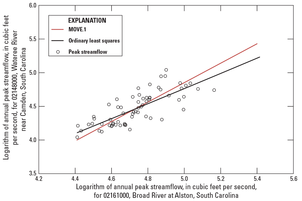
Graph showing Maintenance of Variance Extension, Type 1 (MOVE.1) and ordinary least squares correlations for U.S. Geological Survey streamgage 02161000, Broad River at Alston, South Carolina (site 393 on fig. 2), and U.S. Geological Survey streamgage 02148000, Wateree River near Camden, South Carolina (site 352 on fig. 9), for water years 1954 through 2019.
As noted earlier at streamgage 02148000, the 1908 flood (366,000 ft3/s) was lower than the 1916 flood (400,000 ft3/s). At streamgage 02161000, neither the 1908 nor 1916 peak flows were measured; however, nearby streamgage data indicate that the 1908 flood would be the peak of record and the 1916 flood would be lower. Consequently, if the 1916 flood at streamgage 02148000 under regulated conditions was estimated directly from the MOVE.1 and OLS relations, the peak flow would have been lower than the 1908 flood. To overcome this discrepancy, the 1916 peak flow at streamgage 02148000 under (estimated) regulated conditions was derived by multiplying the estimated regulated flood for 1908 by the ratio of the unregulated 1916 and 1908 peaks: 218,000 × (400,000/366,000) = 238,000 ft3/s. For the EMA analysis, lower and upper perception thresholds of 238,000 ft3/s and infinity, respectively, were used for the periods from 1886 through 1907, from 1909 through 1915, and from 1917 through 1953, reflecting the range of flows that would have been measured had these flows resulted during those periods (England and others, 2019).
The peak flows at streamgage 02146000, Catawba River near Rock Hill, S.C. (site 344 on fig. 9), include unregulated peak flows from 1896 through 1903 and regulated flows from 1942–2019. Streamgage 02147000, Catawba River below Catawba, S.C., has a peak-flow record from 1968 through 1991. Streamgage 02147020, Catawba River below Catawba, S.C. (site 348 on fig. 9), has a peak-flow record from 1993 through 2019. The difference in the drainage area between streamgages 02147000 and 02147020 is less than 1 percent. Therefore, for the flood‑frequency analysis, the peak flows at these two streamgages were combined and are hereafter referred to as streamgage 02147020.
From the peak-flow record at streamgage 02148000, which is downstream from streamgage 02146000, and other historical records (American Meteorological Society, 2021), the 1908 and 1916 floods would have also been floods of record at streamgages 02146000, Catawba River near Rock Hill, S.C., and 02147020, Catawba River below Catawba, S.C. Therefore, techniques like those used to estimate the magnitude of the 1908 and 1916 peak flows at streamgage 02148000, under current regulated conditions, were used to estimate those peak flows at streamgages 02146000 and 02147020.
As was performed for streamgage 02148000, both MOVE.1 and OLS analyses were performed using concurrent periods of record at streamgages 02146000 and 02147020. For streamgage 02146000, the SMC analysis indicated that peak-flow patterns have been stable since about 1964. A double-mass curve analysis of the peak flows from 1964 through 2019 for streamgages 02146000 and 02161000 also indicated a stable relation. Therefore, the concurrent peaks from 1964 through 2019 were used in the correlation analyses to estimate the 1908 peak at streamgage 02146000 for current regulation conditions. Like streamgage 02148000, extrapolation of the MOVE.1 analysis and OLS analysis interpolation lines was necessary to estimate the 1908 peak, and the mean of the two estimates (137,000 ft3/s) was used. The 1916 peak adjusted for current regulation conditions was estimated by multiplying the 1908 peak by the ratio of the unregulated 1916 and 1908 peaks at streamgage 02148000: 137,000 × (400,000/366,000) = 150,000 ft3/s. The 1908 and 1916 peaks adjusted for current regulation were included in the EMA analysis as historic peaks. Lower and upper perception thresholds of 150,000 ft3/s and infinity, respectively, were used from 1897 through 1907, from 1909 through 1915, and from 1917 through 1963, indicating the range of regulated flows that would have been measured had they resulted during those periods (England and others, 2019).
For streamgage 02147020, the SMC analysis indicated that peak-flow patterns have been stable for the period of record from 1968 through 1991 and from 1993 through 2019. MOVE.1 and OLS correlation analyses were done using the concurrent peak flows from streamgages 02147020 and 02161000. Like streamgages 02148000 and 02146000, extrapolation of the MOVE.1 and OLS lines was necessary to estimate the 1908 peak flow, and the mean of the two estimates (176,000 ft3/s) was used. The 1916 peak adjusted for current regulation conditions was estimated by multiplying the 1908 peak by the ratio of the unregulated 1916 and 1908 peaks at streamgage 2148000: 176,000 × (400,000/366,000) = 192,000 ft3/s. The 1908 and 1916 peaks adjusted for current regulation conditions were included in the EMA analysis for streamgage 02147020 as historic flow peaks. Lower and upper perception thresholds of 192,000 ft3/s and infinity, respectively, were used for the period from 1909 through 1915 and from 1917 through 1967 indicating the range of regulated flows that would have been measured had these flows resulted during those periods (England and others, 2019).
Congaree River
The Congaree River is formed by the convergence of the Saluda and Broad Rivers at Columbia, S.C., with the Broad River Basin encompassing about two-thirds of the drainage basin and the Saluda River about one-third (Conrads and others, 2008). At high streamflows, the Broad River is essentially unregulated because of the limited storage capacity of the various dams and reservoirs throughout the Basin. Streamflows in the Saluda River are appreciably regulated by the Saluda Dam, which was completed in 1929, and to a lesser degree by the Lake Greenwood Dam, which was completed in 1940. Streamgage 02169500, Congaree River at Columbia, S.C. (site 408 on fig. 9), has one of the longest peak-flow records of all the USGS streamgages in South Carolina. Peak flows are available from 1892 through 2019 with a historic peak-gage height from 1852. The peak of record of 354,000 ft3/s at 02169500 occurred in August 1908. Comparing the 1852 and 1908 peak gage-heights indicates that the 1908 peak flow was the largest flood since at least 1852. The previous rural flood‑frequency estimates for streamgage 02169500 published in Feaster and others (2009) were from a letter of final determination for the Congaree River flood-hazard study issued in August 2001 by the Federal Emergency Management Agency (FEMA; 2002) and were based on peak-flow data through 1998. To be consistent with the FEMA flood‑frequency analysis from 2001, similar statistical techniques were used to update the flood‑frequency analyses at streamgage 02169500 using peak-flow data through 2019. An SMC analysis indicated that the slope of the curve decreased about 1930 and has remained relatively stable since that time. A double-mass curve for the concurrent period of record at streamgages 02169500 and 02161000 also shows a stable relation between the peak flows at the two streamgages since about 1930. Concurrent peak flows from 1930 through 2019 were used to generate a Maintenance of Variance Extension, Type 2 (MOVE.2) correlation. A 0.95 correlation coefficient for the peak flows was determined. The MOVE.2 correlation method was used instead of MOVE.1 because MOVE.2 was used in the FEMA flood‑frequency analysis from 2001. A comparison of peak-flow estimates from the MOVE.1 and MOVE.2 lines indicated that the results were essentially the same. Using peak flows from streamgage 02161000, the MOVE.2 line was used to estimate regulated peaks at streamgage 02169500 from 1897 through 1907 and from 1926 through 1928. Using the MOVE.2 estimated regulated peaks at streamgage 02169500 and the unregulated measured peaks at streamgage 02169500, an OLS relation was developed that was used to convert the unregulated peaks from 1892 through 1896 and from 1908 through 1925 to regulated peaks. The converted peaks were then combined with the measured peaks from 1930 through 2019 and included in the regulated peak-flow analysis. Lower and upper perception thresholds of 358,000 ft3/s and infinity, respectively, were used from 1852 through 1891.
North Carolina
Weaver and others (2009) published streamgage flood‑frequency estimates for 49 streamgages in North Carolina known or considered to have regulated and (or) channelized periods of record through water year 2006. Updated flood‑frequency estimates were computed for 33 of these 49 streamgages using the regulated periods of record through water year 2019. The 33 sites include 31 streamgages where the flood‑frequency estimates were previously published in Weaver and others (2009) and 2 streamgages (02091814, Neuse River near Fort Barnwell, N.C. [site 150 on fig. 9], and 0351706800, Cheoah River near Bearpen Gap near Tapoco, N.C. [site 983 on fig. 9]) previously lacking sufficient record to derive flood‑frequency estimates.
Of the 49 streamgages, 18 streamgages with previously published flood‑frequency estimates (Weaver and others, 2009) were not updated during this study because of the following reasons:
-
1. Nine streamages were reclassified from having regulated peaks to unregulated peaks using Benson (1962) criterion of usable storage of less than 103 acre-feet per square mile on altering peaks. The nine streamgages include 02068500, 02082506, 02090500, 02116500, 02120500, 02122500, 0345577330, 03456100, and 03460795 (sites 47, 87, 140, 256, 263, 270, 902, 903, and 910 on fig. 2).
-
2. Two streamgages (02053500 and 02084160, sites 23 and 101 on fig. 2) were reclassified from channelized to unregulated. Plots indicated that the streamgage flood‑frequency estimates were within the range of streamgage statistics of unregulated streamgages included in the preliminary regression analyses. The basins for both Coastal Plain streamgages include a large percentage of agricultural land uses. The historical presence of channelization was deemed no longer a sufficient reason for not including these two streamgages for the purposes of flood‑frequency analyses.
-
3. One streamgage (02087570) was deleted from further publication of flood‑frequency estimates because of continuing issues related to the availability and consistency of the regulated period of record following construction of Falls Lake upstream from the streamgage. Previously published streamgage flood‑frequency estimates (Weaver and others, 2009) for this streamgage are considered rescinded effective upon the publication of this report.
-
4. Six streamgages were deleted from further publication of flood‑frequency estimates because of less than 20 water years of annual peak flows for the regulated period. The six streamgages include 02098198, 02113500, 02119400, 0213903612, 03515000, and 03548000.
Neuse River Basin
For streamgage 02087183, Neuse River near Falls, N.C. (site 124 on fig. 9), the maximum annual peak flow of record (23,300 ft3/s) resulted during water year 1945 prior to regulation. To adjust the 1945 peak to account for regulation, three MOVE.1 analyses were completed using the annual peak flows for the regulated period (water years 1981–2019) at streamgage 02087183 and concurrent peaks from three nearby unregulated streamgages (02081500 Tar River near Tar, N.C. [site 81 on fig. 2B]; 02083500, Tar River at Tarboro, N.C. [site 98 on fig. 2]; and 02085500 Flat River at Bahama, N.C. [site 115 on fig. 2B]). A common challenge in this type of analysis is finding a nearby streamgage with drainage area within plus or minus 50 percent of the drainage area of the streamgage of interest. Correlation coefficients for these three analyses using the three unregulated streamgages were 0.71, 0.40, and 0.68, respectively. Unregulated peaks for water year 1945 (highest since 1919) were adjusted to reflect current regulated conditions resulted in peak-flow predictions of 7,350 ft3/s, 7,390 ft3/s, and 8,900 ft3/s for streamgages 02081500, 02083500, and 02085500, respectively. The two relations (streamgages 02081500 and 02085500) with an approximate correlation coefficient of 0.70 were selected to average the regulation equivalent values of 7,350 ft3/s and 8,900 ft3/s. This resulted in the average of 8,120 ft3/s (rounded down to 8,000 ft3/s for the perception threshold used in the PeakFQ specification file). This rounded average peak flow compared favorably with the range of observed maximum peak flows since the period of regulation began. The average streamflow of 8,000 ft3/s was then used to set a perception threshold for water years 1919–80 for the flood‑frequency analysis at this site. The resulting probability curve indicates the five lowest peak flows were censored per the MGBT procedure.
The passage of Hurricane Matthew across parts of North Carolina during October 2016 resulted in new record peak flows measured at the Neuse River streamgages near Goldsboro (02089000, site 136 on fig. 2B) and at Kinston (02089500, site 138 on fig. 2B). The second highest peak flow on record also was measured further downstream at the streamgage near Fort Barnwell (02091814, site 150 on fig. 9). Comparisons of the new record peak flow with the unregulated period through water year 1980 at the Goldsboro and Kinston streamgages (02089000 and 02089500, respectively) also indicate the water year 2017 peak was higher than peaks measured during the unregulated period, including those years where only a historic peak stage value is available. With the availability of EMA methods in Bulletin 17C techniques, it was deemed appropriate to use the peak flows measured following passage of Hurricane Matthew to set a perception threshold to include the unregulated period as part of the historical record in the flood‑frequency analyses. For streamgage 02089000, the 2017 water year peak flow of 53,400 ft3/s was used to set a perception threshold dating back to 1866, its first year of historic record. For streamgage 02089500, the 2017 water year peak flow of 38,200 ft3/s was used to set a perception threshold dating back to 1919, the first year of historic record for this streamgage at Kinston. Similarly, a perception threshold dating back to 1919 (based on upstream flow data at the Kinston streamgage 02089500) was set for streamgage 02091814 with only a regulated period of record since water year 1997. However, the water year 2017 peak flow of 49,400 ft3/s (measured value) was used for the threshold as opposed to the peak flow of record of 57,200 ft3/s (estimated value) following the passage of Hurricane Floyd in September 1999.
Streamgage 02090380, Contentnea Creek near Lucama, N.C. (site 139 on fig. 9), is located immediately downstream from Buckhorn Reservoir in western Wilson County. The original dam was completed in November 1976, with the reservoir initially being filled in December 1976 (capacity of 133,680,000 cubic feet). Construction of a new larger and taller dam downstream from the original structure was completed in July 1999, and the reservoir was filled by mid-September 1999 because of heavy tropical rains from Hurricane Floyd. Flow releases from the new dam resulted in a new record peak flow of 24,000 ft3/s in September 1999 at the Lucama streamgage (02090380). Construction of the new dam resulted in an almost sevenfold increase in reservoir capacity to 909,000,000 cubic feet (Walter and others, 2006). For the drainage area of 161 mi2 at streamgage 02090380, the higher volume results in a usable storage computed to about 130 acre-feet per square mile (table 8 from Kolb and others, 2023). However, the slopes of the SMC before and after 1999 appear similar, suggesting that the increase in impounding capacity has not had a substantial effect on the peak flows. Further, the slope of the SMC before and after the start of regulation (water year 1977) also are similar indicating no substantial change in peak-flow patterns after regulation. The similarity in the slopes of the SMCs indicates that the use of the complete period of record in the flood‑frequency flow at this streamgage is both appropriate and reasonable. Photographs indicate the outlet is a concrete spillway with no gates, and, thus, water spilling over the crest of the dam would flow with no means of regulation (Hazen and Sawyer, 2022). These observations explain why the peak-flow patterns as indicated by the SMCs for the three periods have been relatively stable throughout period of record at this streamgage (02090380). For the flood‑frequency analysis completed during this study, the entire period of record (water years 1965–2019) was used for this streamgage.
Cape Fear River Basin
Streamgage 02094500, Reedy Fork near Gibsonville, N.C. (site 168 on fig. 9), is located downstream from Lake Townsend and various other upstream impoundments across northern Guilford County. The full period of systematic record dating back to water year 1929 is coded as regulated in the annual peak-flow record in the NWIS peak-flow file for this streamgage (U.S. Geological Survey, 2019). As the record peak flow of 11,600 ft3/s (water year 1947) is higher than the historic water year 1916 peak flow of 8,640 ft3/s, the record peak was used to set a perception threshold for 1917–28 pre-systematic period to increase the overall period of record used in the flood‑frequency analysis for this streamgage.
For streamgage 02102500, Cape Fear River at Lillington, N.C. (site 196 on fig. 9), the maximum annual peak flow of record (150,000 ft3/s) was measured during water year 1945 prior to regulation. To adjust the 1945 peak to account for regulation, a MOVE.1 analysis was completed using upstream streamgage 02102000, Deep River at Moncure, N.C. (site 194 on fig. 2), as the reference index streamgage. A strong correlation coefficient of 0.94 between concurrent annual peak flows at these two streamgages for water years 1981–2019 resulted in an estimated “regulation equivalent” peak flow of 82,700 ft3/s for water year 1945. This estimated peak flow was used to set a perception threshold for the unregulated period during water years 1924–80, which provided for a longer overall historic period in the flood‑frequency analysis for streamgage 02102500.
The passage of Hurricane Florence across parts of North Carolina during September 2018 resulted in new record peak flows measured at the Cape Fear streamgages at the lock and dams near Tarheel (02105500, site 207 on fig. 2) and near Kelly (02105769, site 210 on fig. 2). Comparison of the new record peak flow with the unregulated peaks at the Tarheel streamgage indicates that the water year 2018 peak was higher than peaks observed during the unregulated period, including those years where only a historic peak stage value is available. Like the approach previously discussed for the three downstream Neuse River streamgages, it was deemed appropriate to use the peak flows observed following passage of Hurricane Florence to set a perception threshold to include the unregulated period as part of the historic record in the flood‑frequency analyses. For streamgage 02105500, the 2018 water year peak flow of 87,400 ft3/s was used to set a perception threshold dating back to 1938, the first year of systematic record for this streamgage near Tarheel. Similarly, for streamgage 02105769, the 2018 water peak flow of 76,700 ft3/s was used to set a perception threshold dating back to 1938 (based on upstream streamgage 02105500).
The most recent reservoir built in North Carolina is Randleman Reservoir, which is a narrow valley impoundment located downstream from the confluence of Muddy Creek and the Deep River near Randleman in northern Randolph County. The drainage area at the dam is 172 mi2. Construction on the reservoir began in 2001, and the reservoir was initially filled in 2003 (Greg Flory, Piedmont Triad Regional Water Authority, oral commun., May 25, 2012). However, subsequent repairs to the dam had to be completed in 2005, and the reservoir was again filled a second time in 2007. The long-term streamgage on the Deep River near Randleman (02099500, site 186 on fig. 2) was discontinued in 2004 because of these repairs. However, two other long-term streamgages are located on the Deep River downstream from the reservoir. Streamgage 02100500, Deep River at Ramseur, N.C. (site 187 on fig. 2; drainage area 349 mi2), and streamgage 02102000, Deep River at Moncure, N.C. (site 194 on fig. 2; drainage area 1,434 mi2), have continuous streamflow records beginning in water years 1923 and 1930, respectively.
Analyses for regulated streamgages completed during this study included assessing potential effects on annual peak flows at the two streamgages on the Deep River described above. Development of an SMC of cumulative peak flows indicates the possibility of these effects beginning in about 2010 arising from flood-control operations at the reservoir. However, the short period of affected record was not sufficiently long enough to reach a definitive conclusion concerning the possible effects of the flood-control operations. A longer period of record (decadal) will be needed to further investigate the potential effects of this recently constructed reservoir on downstream peak flows. For the purposes of this study, the streamgage flood‑frequency estimates determined for these two streamgages were based on the entire period of record through water year 2017 and were included in the unregulated group of streamgages used in the regression analyses completed for the study of the Catawba River Basin.
At streamgage 02142500, Catawba River at Catawba, N.C. (site 333 on fig. 9), in Catawba County, the annual peak flow consists of regulated systematic period of record from water years 1936 through 1962. Effects of regulated flows upstream from this streamgage are attributed to multiple impoundments along the Catawba River, dating back to 1915 (Lookout Shoals Lake). The annual peak-flow record includes a historic peak stage of 44.1 ft (peak flow not determined) associated with the 1916 flood resulting across western North Carolina (Paulson and others, 1991). The water year 1940 peak flow of 198,000 ft3/s (peak stage of 36.80 ft) was the peak of record for the systematic regulated period. From comparison of the peak stages from 1916 and 1940, the 1916 peak flow would have been greater than 198,000 ft3/s, and therefore, a perception threshold of 198,000 ft3/s was used for the pre-systematic period from 1915 to 35. The 1916 peak flow also was coded as “greater than” the same water year 1940 peak flow in the PeakFQ specification file (U.S. Geological Survey, 2022). However, based on analyses completed downstream from regulated streamgages on the Catawba and Wateree Rivers (streamgages 02146000 and 02148000, respectively) with long-term (greater than 30 years) systematic records through water year 2019, it was further deemed appropriate to set an additional perception threshold for the post-systematic record (1963–2019) at streamgage 02142500 using the water year 1940 peak flow because the 1916 peak flow at those two streamgages was the peak of record under regulated conditions through water year 2019. Examination of the ranges in downstream systematic records provided a level of confidence to include this additional perception threshold indicating the likelihood that annual peak flows have not exceeded 198,000 ft3/s since the last year (water year 1962) of systematic record at streamgage 02142500.
Estimation of Flood Magnitude and Frequency at Ungaged Sites
A regional regression analysis (Farmer and others, 2019) was used to develop a set of equations for use in estimating the magnitude and frequency of floods for rural ungaged sites in Georgia, South Carolina, and North Carolina with no or minor effects from regulation on peak flows. These equations relate the 50‑, 20‑, 10‑, 4‑, 2‑, 1‑, 0.5‑, and 0.2‑percent AEP streamflows computed from available records for streamgages to selected basin characteristics for the streamgages included in tables 1 and 3 from Kolb and others (2023). The general equation for an OLS regression analysis is of the form
whereQp
is as previously defined;
A, B, C
are explanatory (independent) variables; and
a, b, c, and d
are regression coefficients.
If the response and explanatory variables are logarithmically transformed, the regression equation has the following form:
where the variables are as previously defined in equation 4. Both logarithmic and arithmetic independent variables were used in this study because the logarithmic transformation of some variables, such as percentage of hydrologic regions, did not improve the linear relation with Qp.Tests for Redundancy
Redundancy results when the drainage basins of two streamgages are nested one within another and similarly sized, leading to concurrent streamflow records. When this redundancy results, the two streamgages nearly have the same hydrologic response to a given storm event and, thus, effectively represent only one spatial observation (Gruber and Stedinger, 2008). To determine if two streamgages provided potentially redundant information, the following three types of information were considered: (1) the distance between basin centroids (a basin centroid is the location of the point within a drainage basin that represents the geometric center of the basin), (2) the ratios of the basin drainage areas, and (3) whether the streamgage records were concurrent.
A standardized distance was used, in part, to determine the likelihood that the streamgages provide redundant information. The standardized distance between two streamgages (i and j), SDij, is defined as follows:
whereDij
is the distance between centroids of basin i and basin j, in miles; and
DAi
is the drainage area at site i, in square miles; and
DAj
is the drainage area at site j, in square miles.
Along with the standardized distance, a drainage-area ratio was used to determine if the drainages associated with streamgages were sufficiently similar in location and size to conclude that the streamgages may provide redundant information for the purposes of developing a regional hydrologic model. The drainage-area ratio, DAR, is defined as follows:
whereDAR
is the maximum (max) of the two values in brackets;
DAi
is the drainage area at site i, in square miles; and
DAj
is the drainage area at site j, in square miles.
Previous studies have suggested that screening thresholds of standardized distance less than or equal to 0.50 miles combined with a drainage-area ratio less than or equal to 5 are appropriate for identifying sites with potentially redundant information (Veilleux, 2009; Mastin and others, 2016); consequently, those screening thresholds were adopted for this study. All possible combinations of streamgage pairs from the 965 streamgages with 10 or more years of unregulated record were considered and, if deemed potentially redundant, one streamgage from the pair was removed from the regression dataset (table 1 from Kolb and others, 2023). If the peak-flow record of the streamgage with the shorter period of record from the redundant pair was within the period of record of the streamgage with the longer peak-flow record, the streamgage with the shorter peak-flow record was removed from the analysis. However, if the peak-flow record of the streamgage with the shorter record was outside of the period of record of the longer peak-flow record streamgage, then both streamgages were used in the analysis. In some cases, if only a portion of the period of record for both streamgages had a substantial overlap (10 or more years), then the record for the longer record streamgage was extended by using the MOVE.1 method of correlation analysis (Hirsch, 1982), and the streamgage with the shorter record was removed from the analysis. Three streamgages for which the MOVE.1 method was used for record extension are listed in table 1 from Kolb and others (2023). Of the 965 streamgages with 10 or more years of unregulated record, 164 (about 17 percent) were removed from the regression dataset because of potential redundancy, leaving a regression dataset composed of data for 801 streamgages.
Exploratory Regression Analysis
For the exploratory regression analysis, OLS regression techniques were used to determine the best regression models for all combinations of basin characteristics and testing of the hydrologic regions that define the study area (fig. 2). In OLS regression, linear relations between the explanatory and response variables are necessary; thus, variables sometimes must be transformed to create linear relations. For example, the relation between arithmetic values of basin drainage area and P-percent AEP streamflow (such as the 1‑percent AEP streamflow) typically is curvilinear; however, the relation between the logarithms of drainage area and the logarithms of P-percent AEP streamflow normally is linear. Homoscedasticity (a constant variance in the response variable over the range of the explanatory variables) about the regression line and normality of the residuals is another assumption for OLS regression. Transformation of the P-percent streamflow and the explanatory variables to logarithms often enhances the homoscedasticity of the data about the regression line (Farmer and others, 2019). Homoscedasticity and normality of residuals were examined in residual plots. Additionally, residuals, which are the difference between the observed and predicted values, were mapped to assess the geographical distribution in the uncertainty of the predictions. If the geographic distribution of residuals shows clustering of positive and (or) negative values, that might suggest having subregions could reduce the uncertainty. Multicollinearity, which is a situation where two or more independent variables are highly correlated with strong linear dependence, was also assessed by the variance inflation factor. A variance inflation factor greater than 10 indicates highly correlated explanatory variables and warrants additional investigation (Montgomery and others, 2012), and a variance inflation factor of less than 5 is preferred (Farmer and others, 2019).
Initial OLS regressions were done for the entire study area for the 1‑ and 10‑percent AEP streamflows using only drainage area as the independent variable. Mapping of the residuals indicated clear regional differences, as was expected based on previous flood‑frequency regression analyses. After determining any clear regional differences, numerous potential regions were tested using the EPA level III and IV ecoregions (Omernik, 1987) and the previous hydrologic regions from Feaster and others (2009), Gotvald and others (2009), and Weaver and others (2009), along with variations of those hydrologic regions. From these exploratory analyses, it was concluded that the hydrologic regions used in the previous regional flood‑frequency analyses for the study area were still appropriate.
Two regions within the total study area (Georgia, South Carolina, and North Carolina) have been identified with flood characteristics that are difficult to define. The first region contains the Okefenokee Swamp in southeastern Georgia (fig. 2). This region is undefined because there are no streamgages to define the magnitude and frequency of floods for the basins that drain into the swamp. Feaster and others (2009) identified a second undefined region in the Upper Three Runs River Basin near the midwestern boundary of South Carolina. Although the area includes two streamgages (02197300 and 02197310, sites 476 and 477 on fig. 2), its flood characteristics are not well defined by the two streamgages. Large sand deposits at the upper end of this basin seem to affect rainfall runoff more than other regions of the Sand Hills. As part of the exploratory analysis, selected AEP streamflows were plotted with drainage area by hydrologic region. On that plot, the AEP streamflows for the Upper Three Runs streamgages tend to plot low on the data cloud of streamgages in the Sand Hills region but are not substantially outside the cloud. Therefore, it was decided that the regression equations for the Sand Hills (hydrologic region 3; see fig. 2) are appropriate for the Upper Three Runs River Basin considered in this study. However, users of the regional regression equations should be aware that these equations will likely tend to over predict AEP streamflows in this area and, where possible and appropriate, weighted AEP streamflows should be used (table 5 from Kolb and others, 2023).
All-possible-subsets regression methods were tested using the candidate explanatory variables shown in table 2 from Kolb and others (2023). The final explanatory variables for the exploratory regression analysis were selected based on primarily five factors, including (1) standard error of the estimate, (2) Mallow’s Cp statistic, (3) statistical significance of the explanatory variables, (4) coefficient of determination (R2), and (5) ease of measurement of explanatory variables (Farmer and others, 2019). Results of the all-possible subsets analysis indicated that drainage area, percentage of hydrologic regions 1, 3, 4, and 5, along with the cross product of drainage area and percentage of hydrologic region 2 were the top candidate explanatory variables. The statistical significance of the cross product of drainage area and percentage of hydrologic region 2 indicates an appreciably different slope for the regression line for hydrologic region 2 as compared to those for the other hydrologic regions.
Regional Regression Equations
Generalized least squares (GLS) regression methods, as described by Stedinger and Tasker (1985, 1986), were used to determine the final regional P-percent AEP flow regression equations using the weighted-multiple-linear regression (WREG) program version 3.0 written in statistical software R (R Core Team, 2020; Farmer, 2021). Stedinger and Tasker (1985, 1986) found that GLS regression equations are more accurate and provide a better estimate of the accuracy of the equations than OLS regression equations when annual peak-flow records at streamgages are of different and widely varying lengths and when concurrent flows at different streamgages are correlated. GLS regression techniques give less weight to streamgages with shorter periods of record than streamgages with longer periods of record. Less weight also is given to streamgages where concurrent peak flows are correlated because of the geographic proximity with other streamgages (Hodgkins, 1999).
For both the OLS and GLS regression analyses, regression diagnostics were computed and reviewed to assess potential problems with the regression models. Along with reviewing the residuals in terms of being randomly distributed around zero and assessing the geographical distribution, regression diagnostics also were reviewed to assess high leverage and high influence metrics. The leverage metric measures how far away the values of independent variables at one streamgage are compared to the values of the same variables at all other streamgages. The influence metric indicates whether the data at a streamgage had a high influence on the estimated regression metric values (Eng and others, 2009; Farmer and others, 2019). A streamgage may have a high leverage metric indicating that its independent variables are substantially different from those at all other streamgages, but the same streamgage may not have a high influence on the regression metrics. Conversely, a streamgage with a high influence may not have a high leverage metric. Sometimes, measurement or transposing errors in reported values of some independent variables may produce high leverage or influence metrics. Streamgages with high influence or leverage metrics were given additional review to determine if such errors had been made or if the streamgage should be excluded for other reasons. Brief notes are included in table 4 from Kolb and others (2023) for the streamgages that were excluded based on reviews of regression diagnostics. For the final regression analyses, 801 streamgages were included, and the distribution by State is shown in table 1 (see also fig. 2). For those 801 streamgages, the distribution of the systematic peak-flow record lengths is shown in figure 11.
Table 1.
Distribution by State of 801 streamgages included in the regional regression analyses for Alabama, Florida, Georgia, North Carolina, South Carolina, Tennessee, and Virginia.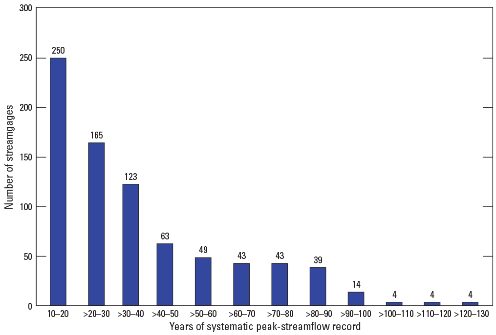
Graph showing distribution of systematic peak-flow record lengths for rural streamgages included in the regional regression analyses for Alabama, Florida, Georgia, North Carolina, South Carolina, Tennessee, and Virginia.
The final set of regression equations for estimating peak flows at the selected AEPs are listed in table 2. The equations allow for the computation of AEP streamflows for unregulated, ungaged rural basins that drain from one or more of the five hydrologic regions (fig. 2), with hydrologic region 4 being the “base” region, which means that at an ungaged location when basin percentages of hydrologic regions 1, 2, 3, and 5 are zero, the site is located 100 percent within hydrologic region 4. Including the percentage of hydrologic region allows for a smooth transition in flood‑frequency estimates among the hydrologic regions. For basins that are 100‑percent contained within one of the five hydrologic regions, the equations are reduced to a simpler form as shown in table 3. Plots of the observed and predicted 10‑ and 1‑percent AEP streamflows are shown in figure 12A and B. The plots indicate a reasonable scatter about the line of equality throughout the range of streamflows. A data release by Weaver and others (2023) provides a model archive of the inputs and outputs for (1) the at-site flood‑frequency statistics and (2) the regression models developed to allow for estimation of flood‑frequency statistics at ungaged stream locations in the study area.
Table 2.
Regional flood‑frequency equations for estimating peak flows at unregulated, ungaged rural locations in Georgia, South Carolina, and North Carolina.[Q50%, Q20%,…, Q0.2%, peak flows with annual exceedance probabilities of 50 percent, 20 percent,…, and 0.2 percent, in cubic feet per second; PCT1, PCT2, PCT3, and PCT5 are the basin percentages in hydrologic regions 1, 2, 3, and 5, in percent; DA, drainage area, in square miles. Note: When PCT1, PCT2, PCT3, and PCT5 are zero, the equation represents sites that are located 100 percent in hydrologic region 4]
Table 3.
Regional flood‑frequency equations for estimating peak flows at unregulated, ungaged rural locations in Georgia, South Carolina, and North Carolina for drainage basins 100‑percent contained within one hydrologic region.[HR, hydrologic region; DA, drainage area, in square miles. Hydrologic regions are shown in figure 2]
Graphs showing the relation between the observed and predicted (A) 10‑ and (B) 1‑percent annual exceedance probability streamflows for Georgia, South Carolina, and North Carolina.
In the simplified equations that represent basins draining 100 percent from a single hydrologic region as a function of drainage area, the regression constant represents the intercept of the regression line, which for logarithmic space results when the drainage area is equal to one. The coefficient for drainage area represents the slope of the regression line. Thus, as can be seen by the equations in table 3, the regression lines for hydrologic regions 1, 3, 4, and 5 have the same slope but different intercepts (fig. 13A). The use of percentage of hydrologic regions as independent variables in the regression equations allows for a smooth transition in the AEP estimates for basins that do not lie wholly within one hydrologic region. The cross product of drainage area and percentage of hydrologic region 2 acts as a “slope adjustment factor” for hydrologic region 2 accounting for the difference in the slope of the regression line from that of the other four hydrologic regions. An example of the transition from a site located 100 percent in hydrologic region 1, represented by the “base” slope (for example, 0.604 for the 1‑percent AEP shown in table 3), to a site located 100 percent in hydrologic region 2 is shown in figure 13B.
Graphs showing rural flood‑frequency relations (A) by hydrologic region for basins 100‑percent contained within one hydrologic region (HR) and (B) for basins in transition from the Piedmont and Ridge and Valley (HR1) to the Blue Ridge (HR2) for Georgia, South Carolina, and North Carolina.
Accuracy and Limitations
Regression equations are statistical models that must be interpreted and applied within the limits of the data and with the understanding that the results are best-fit estimates with an associated scatter or variance. Errors in the model (that is, differences between the predicted and observed values) can be examined to determine parameters that describe the accuracy of a regression equation, which depends on both the model error and the sampling error. Model error measures the capacity of a set of explanatory variables to estimate the values of peak-flow characteristics calculated from the streamgage records used to develop the regression equation. The model error depends on the number and predictive power of the explanatory variables in a regression equation. Sampling error measures the capacity of a finite number of streamgages with a finite number of recorded annual peak flows to describe the true characteristics of the entire peak-flow record for a streamgage. The sampling error depends on the number and record length of streamgages used in the analysis and decreases as the number of streamgages and record lengths increase. A measure of the uncertainty in a regression-equation estimate for a site, i, is the variance of prediction, Vp,i. The Vp,i is the sum of the model-error variance and sampling-error variance and is computed using the following equation:
whereγ2
is the model-error variance, in logarithmic units; and
MSEs,i
is the sampling mean square error for site i, in logarithmic units.
Assuming that the explanatory variables for the streamgages in a regression analysis are representative of all streamgages in the hydrologic region, the average accuracy of prediction for a regression equation can be determined by computing the average variance of prediction, AVP, for n number of streamgages:
A more traditional measure of the accuracy of P-percent AEP streamflow regression equations is the standard error of prediction, Sp, which is simply the square root of the variance of prediction. The average standard error of prediction for a regression equation can be computed in percent error using AVP, in log units, and the following transformation formula:
whereThe Sp,ave is a measure of the average accuracy of the regression equations when predicting flood estimates for ungaged sites, which is the most common application of the regression equations. There is about a 68‑percent probability that the true AEP streamflow at an ungaged location will be between plus or minus the Sp,ave of the regression estimate (Hodgkins, 1999).
A measure of the proportion of the variation in the response variable explained by the explanatory variables in OLS regressions is the coefficient of determination, R2 (Montgomery and others, 2012). For GLS regressions, a more appropriate performance metric than R2 is the pseudo coefficient of determination, pseudo R2, described by Griffis and Stedinger (2007). Unlike the R2 metric, pseudo R2 is based on the variability in the response variable explained by the regression after removing the effect of the time-sampling error. The pseudo R2 is computed using the following equation:
whereγ2(k)
is the model-error variance from a GLS regression with k explanatory variables; and
γ2(0)
is the model-error variance from a GLS regression with no explanatory variables.
The average variance of prediction, average standard error of prediction, and pseudo R2 for the final set of regional regression equations are listed in table 4.
Table 4.
Annual exceedance probability, pseudo coefficient of determination (pseudo R2), average variance of prediction, and average standard error of prediction for the rural regional regression equations for Georgia, South Carolina, and North Carolina.Users of the regression models given above may be interested in a measure of uncertainty at a particular ungaged site as opposed to the uncertainty statistics based on streamgage data used to generate the regression models. One such measure of uncertainty at a particular ungaged site is the confidence interval of a prediction, or prediction interval. Prediction interval is the minimum and maximum value between which a stated probability that the true value of the response variable is present. Tasker and Driver (1988) determined that a 100 (1–α) prediction interval for the true value of a streamflow statistic for an ungaged site from the regression equation can be computed as follows:
whereQ
is the streamflow characteristic for the ungaged site, and
C
is confidence or prediction interval computed as
Z(α/2)
is the normal critical value at a particular alpha-level α, which is the probability that the prediction interval will not contain the true value, equals 0.05 for a 95‑percent prediction interval, divided by 2 and is equal to 1.96 for an α of 0.05; and
Sp,i
is the standard error of prediction and is computed as
γ2
is the model-error variance;
xi
is a row vector of variables log DA, PCT1, PCT3, PCT5, and log DA× PCT2 for site i, augmented by a 1 as the first element;
U
is the covariance matrix for the regression coefficients;
xi′
is the transpose of xi (Ludwig and Tasker, 1993);
DA
is drainage area in square miles;
PCT1
is the basin percentage in hydrologic region 1;
PCT2
is the basin percentage in hydrologic region 2;
PCT3
is the basin percentage in hydrologic region 3; and
PCT5
is the basin percentage in hydrologic region 5.
The values for γ2 and U are presented in table 9 from Kolb and others (2023).
The following limitations should be considered when using the final regional regression equations for Georgia, South Carolina, and North Carolina:
-
1. The ranges of explanatory variables used to develop the regional regression equations are shown in figure 14 and table 5. Because the regression analyses included the percentage of hydrologic regions as an independent variable, the accuracy estimates and use of the relations are considered appropriate for basins contained within one hydrologic region or draining from multiple hydrologic regions throughout the ranges of the independent variables shown.
-
2. The methods are not appropriate (or applicable) for sites where the watershed is affected substantially by regulation from impoundments, channelization, levees, or other manmade structures.
-
3. The methods are not applicable for sites on streams in urban areas (impervious area greater than 10 percent).
-
4. The methods do not apply where flooding is affected by extreme ocean storm surge or tidal events.
-
5. The methods are not valid for streams in the undefined area on figure 2A containing the Okefenokee Swamp in southeastern Georgia, where the magnitude and frequency relations are undefined.
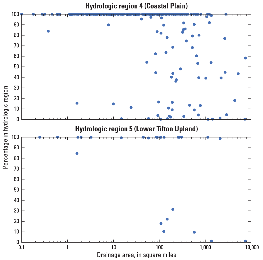
Graphs showing distribution of drainage areas by hydrologic region for sites with a percentage of basin within the indicated region for Georgia, South Carolina, and North Carolina.
Table 5.
Range of drainage area and percentage of hydrologic regions used to develop the regression equations for rural streams in Georgia, South Carolina, and North Carolina.[HR, hydrologic region; min, minimum; max, maximum; mi2, square miles. Hydrologic regions are shown in figure 2]
Comparison of Regression Results with Previous Rural Flood‑frequency Study
Flood‑frequency estimates at streamgages and regional flood‑frequency equations developed from those streamgage estimates contain uncertainty based on numerous factors, such as length of streamgage record, hydrologic conditions represented by the streamgage records, number of streamgages included in the regionalization, and range of the basin characteristics included in the regionalization. For flood‑frequency estimates computed from peak flows at specific streamgages, Benson and Carter (1973) showed that the standard error tends to be reduced as the period of record increases. Dalrymple (1960) generated 1,000 peak-flow events and then divided the events into various consecutive periods of record including one hundred 10‑year periods, forty 25‑year periods, twenty 50‑year periods and ten 100‑year periods. For each set of data, flood‑frequency curves were then drawn on the same graph for each period resulting in frequency plots of 100, 40, 20, and 10 curves, respectively. For the ten 100‑year curves, the estimates of the 100‑year recurrence interval flow ranged from about 6,500 to 9,200 ft3/s, reflecting the variation in such estimates just based on sampling from different time periods (time-sampling error).
Updating the regional skew also will affect the flood‑frequency estimates at a streamgage. The regional skew from the previous rural flood‑frequency study for Georgia, South Carolina, and North Carolina by Feaster and others (2009), Gotvald and others (2009), and Weaver and others (2009), respectively, used a regional skew of −0.019 with a mean square error (MSE) of 0.143. The updated regional skew was 0.048 with an MSE of 0.092, which also is noted as the average variance of prediction in appendix 1. In addition, the previous study was based on techniques from Bulletin 17B (Interagency Advisory Committee on Water Data, 1982) whereas, the current study is based on updated techniques in Bulletin 17C (England and others, 2019).
The 10‑ and 1‑percent AEP streamflow-regression lines developed from this study were compared with the regression lines from the previous rural flood‑frequency study for Georgia, South Carolina, and North Carolina (figs. 15 and 16; Feaster and others, 2009; Gotvald and others, 2009, and Weaver and others, 2009). For the comparisons, the simplified equations that are only a function of drainage area were used (table 3). The 10‑ and 1‑percent AEP streamflows were computed using the simplified equations from the current and previous studies for streamgages in Georgia, South Carolina, and North Carolina that drain 100 percent from a single hydrologic region and were included in the regression analyses for this study (table 1 from Kolb and others, 2023). The percentage change ([current − previous]/previous) of the 10‑ and 1‑percent AEP streamflows for the streamgages meeting this criterion were computed and the mean and median values for each hydrologic region are shown in table 6.
Table 6.
Comparison of 10‑ and 1‑percent annual exceedance probability streamflows from the current study and from the previous rural flood‑frequency study for Georgia, South Carolina, and North Carolina.[AEP, annual exceedance probability; HR, hydrologic region; Previous study data are from Feaster and others (2009), Gotvald and others (2009), and Weaver and others (2009). Hydrologic regions are shown in figure 2]
Graph showing predicted 10‑percent annual exceedance probability streamflow regression lines by drainage area for hydrologic regions (HRs) 1–5 from this study and corresponding regression lines from the previous rural flood‑frequency study (Feaster and others, 2009; Gotvald and others, 2009; and Weaver and others, 2009) for Georgia, South Carolina, and North Carolina.
Graph showing predicted 1‑percent annual exceedance probability streamflow regression lines by drainage area for hydrologic regions (HRs) 1–5 from this study and corresponding regression lines from the previous rural flood‑frequency study (Feaster and others, 2009; Gotvald and others, 2009; and Weaver and others, 2009) for Georgia, South Carolina, and North Carolina.
The percentage differences in hydrologic regions 1 and 2 were considered reasonable when comparing regression equations generated from two sets of data for two different time periods (table 6). The largest percentage differences were for the streamgages in Sand Hills hydrologic region (HR3). In the past decade, there have been several historical flood events that impacted the Sand Hills and Coastal Plain regions (Feaster and others, 2015, Feaster, Weaver, and others, 2018; Weaver and others, 2016), which would influence the updated regression equations. In the previous study, the regression lines for the Blue Ridge and Sand Hills regions exhibited a different slope than the other regions. In the current study, the Blue Ridge regression line still has a different slope, but the Sand Hills does not (fig. 13A). As such, the divergence of the regression lines for the Sand Hills region below 100 mi2 is accounting for much of the difference between the current and previous regression estimates (figs. 15 and 16), which also is likely related to the historical flooding previously noted. It should also be noted that HR3 has a smaller number of streamgages than the other hydrologic regions except for HR5, which makes the regression lines more sensitive to changes in the at-site statistics used in the regression analysis. The historical flooding also is likely a strong influence in the increase in regression estimates for the Coastal Plain hydrologic region (HR4).
The mean and median percentage changes in the 10‑ and 1‑percent AEP regression estimates for streamgages in the Lower Tifton Upland region (HR5) were the second largest of the five hydrologic regions in this study (table 6). In the spring of 2009, historical flooding occurred in southern Georgia in the area that includes HR5 (Gotvald, 2010), with many streamgages having peak flows exceeding the 1‑ and 0.2‑AEP streamflows. As such, and like the Sand Hills and Coastal Plain regions, that historical flooding is likely a strong influence in the increase in the regression estimates for HR5.
Maximum Floods
In a flood‑frequency analysis, it is inherent that for floods with a specified probability of recurrence (such as the 1‑percent AEP streamflows), the regression line is a best-fit line for linear regression (or a best-fit plane for multiple regression) through a series of statistically specified P-percent AEP streamflows from some number of gaged locations in a given region. The regression line is fit so that the variance about the line is minimized; therefore, approximately half of the data points will plot above the regression line and half will plot below the regression line. For many engineering design projects, this level of uncertainty is acceptable and often is compensated for by including a factor of safety in the design process. In certain projects that include concerns about high risk, the assessment of maximum measured floods is another tool that can be used to evaluate the reasonableness of a flood‑frequency estimate.
Crippen and Bue (1977) developed envelope curves, which are curves encompassing the maximum values in a dataset, from maximum flood data for 17 regions in the conterminous United States (fig. 17). Crippen (1982) later provided equations that described the envelope curves. The curves were not associated with specific probabilities or frequencies but were provided as a tool to help assess the maximum flood that might be expected in the regions for a given drainage-area size. Costa (1987) developed an envelope curve of the maximum rainfall-runoff floods in the United States, but his dataset did not include any streamgages in the southeastern United States.
Maximum peak flows were plotted with drainage area using data from the streamgages included in table 1 from Kolb and others (2023) (figs. 18 and 19). In addition, a few streamgages that currently are regulated but had appreciable large floods recorded prior to regulation also were included (table 10 from Kolb and others, 2023). The streamgages were grouped based on having at least 75 percent of the basin located either above or below the Fall Line (fig. 1), which allows for comparisons with the Crippen (1982) curves. An envelope curve was then drawn for both regions that encompasses the largest floods. The streamgages above the Fall Line include data from the Ridge and Valley, Blue Ridge, and Piedmont ecoregions, and the streamgages below the Fall Line include data from the Southeastern Plains, Middle Atlantic Coastal Plain, and Southern Coastal Plain ecoregions (fig. 1). Similar to the Crippen (1982) curves, the envelope curves generated from the maximum flow data included in this study indicate maximum flood-streamflow potential for a range of drainage areas for the two regions, which are (1) the area above the Fall Line and (2) the area below the Fall Line (table 7).
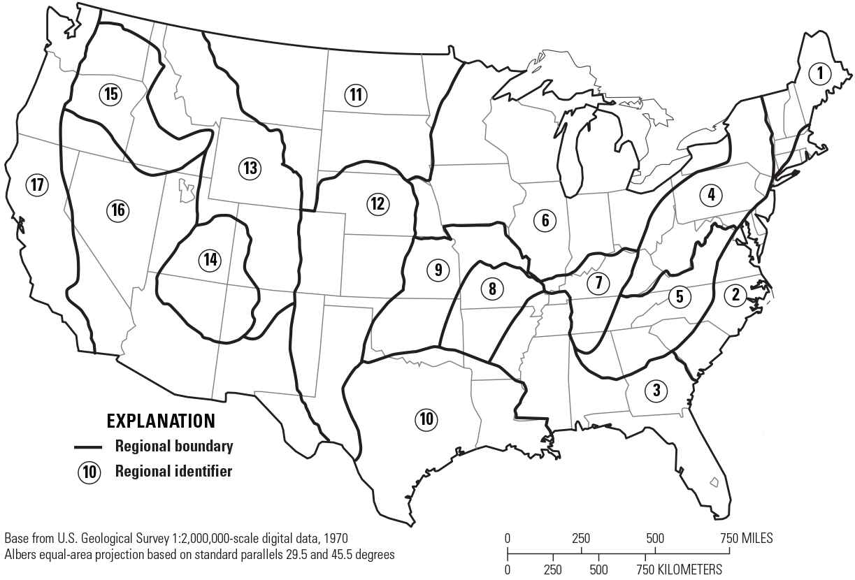
Map showing flood-region boundaries within the conterminous United States (Crippen, 1982).
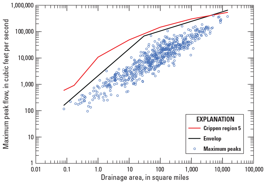
Graph showing maximum peak flow and drainage area for streams located above the Fall Line in Georgia, South Carolina, and North Carolina. Crippen region 5 is from Crippen (1982).
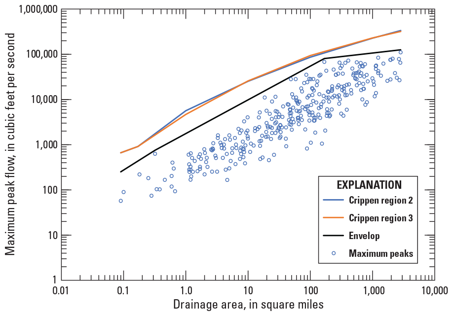
Graph showing maximum peak flow and drainage area for streams located below the Fall Line in Georgia, South Carolina, and North Carolina. Crippen regions 2 and 3 are from Crippen (1982).
Application of Flood‑frequency Methods
The best estimates of flood frequencies for a site typically are obtained through a weighted combination of estimates produced from more than one method. The following sections describe the weighting process for a streamgage and an ungaged site on the same river with a nearby streamgage in more detail and provide example calculations. The results are rounded to three significant figures.
Flood‑frequency Estimation at a Streamgage
Bulletin 17C (England and others, 2019) recommends that better flood‑frequency estimates for a streamgage can be obtained by combining (weighting) streamgage flow estimates determined from the log-Pearson Type III analysis of the annual peaks with flow estimates obtained for the streamgage from regression equations. Optimal weighted flow estimates can be obtained if the variance of prediction for each of the two estimates is known or can be estimated accurately and precisely. The variance of prediction can be thought of as a measure of the uncertainty in either the streamgage estimate or the regional regression results. If the two estimates can be assumed independent and are weighted in inverse proportion to the associated variances, the variance of the weighted estimate will be less than the variance of either of the independent estimates.
The variance of prediction corresponding to the streamgage flow estimate from the LPIII analysis is computed using the asymptotic formula given in Cohn and others (2001) with the addition of the mean-squared error of generalized skew (Griffis and others, 2004). This variance varies as a function of the length of record, the fitted LPIII distribution parameters (mean, standard deviation, and weighted skew), and the accuracy of the method used to determine the generalized skew component of the weighted skew. The variance of prediction for the streamgage estimate generally decreases with length of record and the quality of the LPIII distribution fit. The variance of prediction values for the streamgage flow estimates for the 807 streamgages in Georgia, South Carolina, and North Carolina are listed in table 3 from Kolb and others (2023), which includes both the redundant streamgages and those included in the regression analyses.
The variance of prediction from the regional regression equations is a function of the regression equations and the values of the independent variables used to develop the flow estimate from the regression equations. This variance generally increases as the values of the independent variables move further from the mean values of the independent variables. For the streamgages included in the regression analysis, the variance of prediction is provided as part of the WREG output (table 3 from Kolb and others, 2023). The average variance of prediction values for the regional regression equations used in this study are listed in table 4 and can be used for weighting of streamflow estimates (eq. 15) for streamgages not included in the regression analysis.
Once the variances have been computed, the two independent flow estimates can be weighted using the following equation:
whereQw(s)
is the weighted estimate of peak flow for any P-percent AEP for a streamgage, in cubic feet per second;
Vr(s)
is the variance of prediction at the streamgage derived from the applicable regional regression equations for the selected P-percent AEP (table 3 from Kolb and others, 2023), in log units, which is obtained from the WREG output. If the weighting is being done for a streamgage that was not included in the WREG regression analysis, the average variance of prediction can be used from table 4;
Qs
is the estimate of peak flow at the streamgage from the LPIII analysis for the selected P-percent AEP, in cubic feet per second;
Vs
is the variance of prediction at the streamgage from the LPIII analysis for the selected P-percent AEP (table 3 from Kolb and others, 2023), in log units; and
Qr(s)
is the peak-flow estimate for the P-percent AEP at the streamgage derived from the applicable regional regression equations in table 2, in cubic feet per second.
The weighted (best) flow estimates were computed using equation 15 along with the variance of prediction values for the regression equations (table 4) and the variance from the at-site EMA analyses for the 807 streamgages in Georgia, South Carolina, and North Carolina (table 3 from Kolb and others, 2023). When the variance of prediction corresponding to one of the estimates is high, the uncertainty is also high and so the weight for that estimate is relatively small. Conversely, when the variance of prediction is low, the uncertainty is also low and so the weight is correspondingly large. The variance of prediction associated with the weighted estimate, Vw(s), is computed using the following equation:
where all the variables are as previously defined.Confidence intervals for the weighted estimate also can be computed. The upper and lower 95‑percent confidence intervals (95%CI) on the weighted AEP estimate can be computed as
where all variables are as previously defined.An example of the application of the procedure described above is the following steps for computation of the weighted 1‑percent AEP streamflow for streamgage 02116500, Yadkin River at Yadkin College, N.C. (site 256 on fig. 2; tables 1 and 3 from Kolb and others, 2023):
-
1. Obtain the streamgage estimate of the 1‑percent AEP flow at the site based on the systematic flood peaks (table 3 from Kolb and others, 2023) (Qs = 84,200 ft3/s);
-
2. Obtain drainage area and hydrologic region percentages (table 1 from Kolb and others, 2023) (DA = 2,278 mi2, PCT1 = 74.7, PCT2 = 25.3, PCT3 = 0, PCT4 = 0, and PCT5 = 0);
-
3. Compute Qr(s) using the 1‑percent AEP equation in table 2: Qr(s) = 10[2.64 + 0.00218(74.7) − 0.00311(0) + 0.00309(0)] 2,278[0.605 + 0.00161(25.3)] = 93,525 ft3/s, which is rounded to 93,500 ft3/s for Qr(s) for this streamgage (table 3 from Kolb and others, 2023);
-
4. Obtain the variance of prediction for the streamgage estimate for the 1‑percent AEP streamflow (table 3 from Kolb and others, 2023) (Vs = 0.0024);
-
5. Obtain the variance of prediction for the 1‑percent AEP streamflow regression equation from table 3 from Kolb and others (2023) (Vr(s) = 0.0293);
-
6. Compute the weighted 1‑percent AEP streamflow for the streamgage using equation 15: log Qw(s) = [(0.0293) (log 84,200) + (0.0024) (log 93,500)] / (0.0293 + 0.0024) = 4.929 (rounded), and the base 10 antilog Qw(s) = 84,918 ft3/s, which is rounded to 84,900 ft3/s for Qw(s) for this streamgage (table 3 from Kolb and others, 2023);
-
7. Compute the weighted 1‑percent chance exceedance variance for the streamgage using equation 16: Vw(s) = (0.0293 × 0.0024) / (0.0293 + 0.0024) = 0.0022; and
-
8. Compute the 95%CI using equation 17:
= [68,700 ft3/s, 105,000 ft3/s] (rounded).
Flood‑frequency Estimation for an Ungaged Site Near a Streamgage
Sauer (1974) presented the following method to improve flood‑frequency estimates for an ungaged site near a streamgage, on the same stream, with 10 or more years of peak-flow record. To obtain a weighted peak-flow estimate (Qw(u)) for P-percent AEP at the ungaged site, the weighted flow estimate for an upstream or downstream streamgage (Qw(s)) must first be determined by using equation 15 provided in the previous section. The weighted estimate for the ungaged site (Qw(u)) is then computed using the following equation:
whereQw(u)
is the weighted estimate of peak flow for the selected P-percent AEP at the ungaged site, in cubic feet per second;
ΔA
is the absolute value of the difference between the drainage areas of the streamgage and the ungaged site, in square miles;
A(s)
is the drainage area for the streamgage, in square miles;
Qr(u)
is the peak-flow estimate derived from the applicable regional equations in table 2 for the selected P-percent AEP at the ungaged site, in cubic feet per second; and
Qw(s) and Qr(s)
are previously defined in equation 15
Use of equation 18 gives full weight to the regression equation estimates when the drainage area for the ungaged site is equal to 0.5 or 1.5 times the drainage area for the streamgage and increasing weight to the streamgage estimates as the drainage-area ratio approaches 1. The weighting procedure should not be applied when the drainage-area ratio for the ungaged site and streamgage is less than 0.5 or greater than 1.5.
An example application of this procedure is the computation of the weighted 1‑percent AEP streamflow for a hypothetical ungaged site on the Yadkin River located above the USGS streamgage 02116500, Yadkin River at Yadkin College, N.C. (site 256 on fig. 2; table 1 from Kolb and others, 2023), discussed in the previous section. The regulated streamgage 02115360, Yadkin River at Enon, N.C. (site 248 on fig. 9; table 8 from Kolb and others, 2023), is used as a hypothetical unregulated and ungaged site for purposes of this example:
-
1. Calculate the value of Qw(s) for the streamgage (see step 6 of example in previous section, Qw(s) = 84,900 ft3/s);
-
2. Obtain the drainage areas for both the gaged and ungaged sites (As = 2,278 mi2 and Au = 1,690 mi2);
-
3. Determine the hydrologic region percentages for the ungaged site (the following percentages were determined for site 248 during the study and are not provided in any table in this report: PCT1 = 66, PCT2 = 34, PCT3 = 0, PCT4 = 0, PCT5 = 0);
-
4. Compute Qr(u) for the ungaged site using the 1‑percent AEP equation in table 2 (Qr(u) = 10[2.64 + 0.00218(66) − 0.00311(0) + 0.00309(0)] 1,690[0.605 + 0.00161(34)] = 81,931 ft3/s, which is rounded to 81,900 ft3/s for Qr(u) for this ungaged site);
-
5. Compute Qr(s) for the streamgage using the 1‑percent AEP equation in table 2 (see step 3 of example in previous section, Qr(s) = 93,500 ft3/s);
-
6. Compute ΔA, where ΔA = 2,278 – 1,690 = 588 mi2; and
-
7. Compute the weighted estimate for the ungaged site, Qw(u) using equation 18 (Qw(u) = [([2 × 588] / 2,278) + ([1 – ([2 × 588] / 2,278)] × [81,900/93,500])] × 81,900 = 76,984 ft3/s, which is rounded to 77,000 ft3/s).
For an ungaged site that is located between two streamgages on the same stream, two flow estimates can be made using the methods and criteria outlined in this section. In addition to evaluating the differences in hydrologic regions of the two streamgages compared to the hydrologic region(s) for the ungaged site, additional hydrologic expertise and judgment may be necessary to determine which of the two estimates (or some interpolation thereof) is most appropriate. Other factors that might be considered when evaluating the two estimates include differences in the length of record for the two streamgages and the hydrologic conditions present during the data-measurement period for each streamgage (that is, whether the time series represents a climatic period that was predominately wet or dry).
StreamStats
The regression equations developed in this study to estimate rural flood‑frequency statistics will be incorporated into the USGS StreamStats application (https://streamstats.usgs.gov/ss/) for Georgia, South Carolina, and North Carolina. USGS StreamStats is a web-based GIS application that provides a range of analytical tools useful for water-resource managers, planners, and engineers (Ries and others, 2017). The StreamStats application can be used to delineate drainage areas, generate basin characteristics, and compute estimates of streamflow statistics for user-selected sites. StreamStats also provides streamflow statistics and other information at USGS streamgages. StreamStats can save users substantial time and resources and provides consistent and accurate basin characteristics and flood‑frequency estimates.
Summary and Conclusions
This report, prepared by the U.S. Geological Survey (USGS) in cooperation with the Georgia, South Carolina, and North Carolina Departments of Transportation and the North Carolina Department of Crime Control and Public Safety, presents methods for determining flood magnitude and frequency at rural streamgages and ungaged sites in Georgia, South Carolina, and North Carolina. For the study described in this report, flood‑frequency estimates of the 50‑, 20‑, 10‑, 4‑, 2‑, 1‑, 0.5‑, and 0.2‑percent annual exceedance probability (AEP) streamflows were computed for 965 streamgages in or near these three States, of which 801 streamgages were included in the regional regression analysis. Streamgages used for this study are in rural basins, have 10 years or more of peak-flow record, and are not significantly appreciably affected by regulation, tidal fluctuations, or urban development. By using a multistate analysis, continuity in hydrologic regions and regression equations at State boundaries is maintained; therefore, there is no confusion on which flood‑frequency techniques and results are most appropriate for drainage basins near or crossing State boundaries.
Peak flows for select annual exceedance probabilities were estimated following new national guidelines for flood‑frequency analyses (Bulletin 17C; England and others, 2019). The new guidelines have improved statistical methods for flood‑frequency analysis including (1) the expected moments algorithm to help describe uncertainty in annual peak flows and to better represent missing and historic records and (2) the generalized multiple Grubbs-Beck test to screen out potentially influential low outliers and to better fit the upper end of the peak-flow distribution. Additionally, a new regional skew was derived for the study area following the new guidelines.
A regional analysis of streamgage skew coefficients resulted in one regional skew coefficient that can be used for the entire study area. The regional skew value of 0.048 was determined for this study using a Bayesian generalized least squares (GLS) regression model (compared to the regional skew value of –0.019 determined for the previous USGS rural flood‑frequency study completed in 2009 (Feaster and others, 2009; Gotvald and others, 2009; Weaver and others, 2009). The mean square error (MSE) for the new regional skew value is 0.092, which is less than the 0.143 MSE for the regional skew determined in the previous USGS study. A weighted skew coefficient (using the streamgage and regional skew values) was used with the log-Pearson Type III analysis to compute the AEP streamflows at each streamgage considered within the study area.
Regional regression analysis, using GLS regression, was used to develop a set of predictive equations that can be used to estimate the 50‑, 20‑, 10‑, 4‑, 2‑, 1‑, 0.5‑, and 0.2‑percent AEP streamflows in Georgia, South Carolina, and North Carolina. The predictive equations are all functions of drainage area and the percentage of drainage basin within each of five hydrologic regions defined in the study area. As such, the predictive equations can be used to estimate the P-percent AEP streamflows for ungaged sites with a drainage basin in one or more of the five hydrologic regions: region 1, Piedmont and Ridge and Valley; region 2, Blue Ridge; region 3, Sand Hills; region 4, Coastal Plain; and region 5, Lower Tifton Upland. Average errors of prediction for these equations ranged from 35.8 to 44.4 percent.
The magnitude and frequency of floods also were computed at 72 regulated streamgages in Georgia, South Carolina, and North Carolina using the streamgage skew. The streamgage skew was used because the regional skew is not representative of regulated peak-flow records. At various streamgages with peak-flow records measured during the unregulated period and for which historic floods were recorded, those historic floods were adjusted to account for current (as of 2019) regulated conditions and included in the flood‑frequency analyses.
A Kendall’s tau trend analysis was completed for the 965 unregulated streamgages included in this report. Of those streamgages, 332 were in operation in 2017 and had 30 or more years of systematic record. Of those 332 streamgages, 276 (83 percent) indicated no statistically significant trend, 45 (14 percent) indicated a downward trend, and 11 (3 percent) indicated an upward trend. The trend results did not offer clear and convincing evidence for incorporating trends into the flood‑frequency analyses performed here. For this study, the assumption of stationarity is used with no adjustments to the annual peak flows for trends.
The updated peak-flow statistics and regional regression equations will be incorporated into the USGS StreamStats application for Georgia, South Carolina, and North Carolina. The StreamStats application generates the needed independent variables for the regression equations, which are drainage area and percentage of basin draining from hydrologic regions 1–5. StreamStats also provides uncertainty statistics with the flood‑frequency estimates. The StreamStats application can save users substantial time and resources and provides consistent and accurate basin characteristics and flood‑frequency estimates.
References Cited
Advisory Committee on Water Information, 2021, Subcommittee on Hydrology, Hydrologic Frequency Analysis Work Group, Bulletin 17–B guidelines for determining flood frequency frequently asked questions: Advisory Committee on Water Information web page, accessed January 11, 2021, at https://acwi.gov/hydrology/Frequency/B17bFAQ.html.
American Meteorological Society, 2021, Monthly weather review: American Meteorological Society web page, accessed January 15, 2021, at https://www.ametsoc.org/index.cfm/ams/publications/journals/monthly-weather-review/.
Conrads, P.A., Feaster, T.D., and Harrelson, L.G., 2008, The effects of the Saluda Dam on the surface-water and ground-water hydrology of the Congaree National Park flood plain, South Carolina: U.S. Geological Survey Scientific Investigations Report 2008–5170, 58 p. [Also available at http://pubs.water.usgs.gov/sir2008-5170.]
Cooney, T.W., Jones, K.H., Drewes, P.A., Gissendanner, J.W., and Church, B.W., 1995, Water resources data—South Carolina, water year 1994: U.S. Geological Survey Water-Data Report SC–94–1, 520 p. [Also available at https://doi.org/10.3133/wdrSC941.]
Eng, K., Chen, Y.-Y., and Kiang, J.E., 2009, User’s guide to the weighted-multiple-linear-regression program (WREGversion 1.0): U.S. Geological Survey Techniques and Methods, book 4, chap. A8, 21 p. [Also available at https://pubs.usgs.gov/tm/tm4a8.]
England, J.F., Jr., Cohn, T.A., Faber, B.A., Stedinger, J.R., Thomas, W.O., Jr., Veilleux, A.G., Kiang, J.E., and Mason, R.R., Jr., 2019, Guidelines for determining flood flow frequency—Bulletin 17C (ver. 1.1, May 2019): U.S. Geological Survey Techniques and Methods, book 4, chap. B5, 148 p. [Also available at https://doi.org/10.3133/tm4B5.]
Farmer, W.H., 2021, WREG—Weighted least squares regression for streamflow frequency statistics (ver. 3.0): U.S. Geological Survey software release, accessed January 22, 2021, at https://doi.org/10.5066/P9ZCGLI1.
Farmer, W.H., Kiang, J.E., Feaster, T.D., and Eng, K., 2019, Regionalization of surface-water statistics using multiple linear regression: U.S. Geological Survey Techniques and Methods, book 4, chap. A12, 40 p., accessed January 2020 at https://doi.org/10.3133/tm4A12.
Feaster, T.D., Clark, J.M., and Kolb, K.R., 2018, StreamStats for South Carolina—A multipurpose water-resources web application: U.S. Geological Survey Fact Sheet 2018–3070, 5 p. [Also available at https://doi.org/10.3133/fs20183070.]
Feaster, T.D., Gotvald, A.J., Musser, J.W., Weaver, J.C., and Kolb, K.R., 2023, Magnitude and frequency of floods for rural streams in Georgia, South Carolina, and North Carolina, 2017—Summary: U.S. Geological Survey Fact Sheet 2023–3011, 6 p., https://doi.org/10.3133/fs20233011.
Feaster, T.D., Gotvald, A.J., and Weaver, J.C., 2014, Methods for estimating the magnitude and frequency of floods for urban and small, rural streams in Georgia, South Carolina, and North Carolina, 2011 (ver. 1.1, March 2014): U.S. Geological Survey Scientific Investigations Report 2014–5030, 104 p. [Also available at http://dx.doi.org/10.3133/sir20145030.]
Feaster, T.D., Shelton, J.M., and Robbins, J.C., 2015, Preliminary peak stage and streamflow data at selected USGS streamgaging stations for the South Carolina flood of October 2015 (ver. 1.1, November 2015): U.S. Geological Survey Open-File Report 2015–1201, 19 p. [Also available at http://dx.doi.org/10.3133/ofr20151201.]
Feaster, T.D., Weaver, J.C., Gotvald, A.J., and Kolb, K.R., 2018, Preliminary peak stage and streamflow data at selected U.S. Geological Survey streamgaging stations in North and South Carolina for flooding following Hurricane Florence, September 2018: U.S. Geological Survey Open-File Report 2018–1172, 36 p. [Also available at https://doi.org/10.3133/ofr20181172.].
Federal Emergency Management Agency, 2002, Flood insurance study, Richland County, South Carolina, and incorporated areas: Washington, DC, Federal Emergency Management Agency, revised February 20, 2002. [Also available at https://map1.msc.fema.gov/data/45/S/PDF/45063CV001.pdf?LOC=a8ac2c97c06674dcf7e28e6acd45161c].
Flynn, K.M., Kirby, W.H., and Hummel, P.R., 2006, User’s manual for program PeakFQ, annual flood frequency analysis using Bulletin 17B guidelines: U.S. Geological Survey Techniques and Methods, book 4, chap. B4, 42 p. [Also available at https://doi.org/10.3133/tm4B4.]
Gotvald, A.J., 2010, Historic flooding in Georgia, 2009: U.S. Geological Survey Open-File Report 2010–1230, 19 p. [Also available at https://pubs.usgs.gov/of/2010/1230/.]
Gotvald, A.J., Feaster, T.D., and Weaver, J.C., 2009, Magnitude and frequency of rural floods in the southeastern United States, 2006—Volume 1, Georgia: U.S. Geological Survey Scientific Investigations Report 2009–5043, 120 p. [Also available at https://pubs.usgs.gov/sir/2009/5043/.]
Gotvald, A.J., and Musser, J.W., 2015, StreamStats in Georgia—A water-resources web application: U.S. Geological Survey Fact Sheet 2014–3027, 2 p. [Also available at http://doi.org/10.3133/fs20143027.]
Griffith, G.E., Omernik, J.M., Comstock, J.A., Lawrence, S., Martin, G., Goddard, A., Hulcher, V.J., and Foster, T., 2001, Ecoregions of Alabama and Georgia [color poster with map, descriptive text, summary tables, and photography]: Reston, Va., U.S. Geological Survey (map scale 1:1,700,000). [Also available at http://ecologicalregions.info/data/al/alga_front.pdf.]
Griffith, G.E., Omernik, J.M., Comstock, J.A., Schafale, M.P., McNab, W.H., Lenat, D.R., MacPherson, T.F., Glover, J.B., and Shelburne, V.B., 2002, Ecoregions of North Carolina and South Carolina: U.S. Geological Survey color poster with map, scale 1:1,500,000. [Also available at www.ecologicalregions.info/htm/ncsc_eco.htm.]
Gruber, A.M., and Stedinger, J.R., 2008, Models of LP3 regional skew, data selection and Bayesian GLS regression, in Babcock, R.W., Jr., and Walton, R., eds., Ahupua’a—Proceedings of the World Environmental and Water Resources Congress, Honolulu, Hawai’i, May 12–16, 2008: Reston, Va., American Society of Civil Engineers, 10 p.
Hazen and Sawyer, 2022, Buckhorn Dam and Reservoir expansion: Hazen and Sawyer web page, accessed April 22, 2022, at https://www.hazenandsawyer.com/projects/buckhorn-reservoir-expansion.
Helsel, D.R., Hirsch, R.M., Ryberg, K.R., Archfield, S.A., and Gilroy, E.J., 2020, Statistical methods in water resources: U.S. Geological Survey Techniques and Methods, book 4, chapter A3, 458 p., https://doi.org/10.3133/tm4a3. [Supersedes USGS Techniques of Water-Resources Investigations, book 4, chapter A3, version 1.1.]
Kendall, M.G., 1938, A new measure of rank correlation: Biometrika, v. 30, nos. 1–2, p. 81–93, accessed July 14, 2015, at http://www.jstor.org/stable/2332226.
Kolb, K.R., Heal, E.N., and Clark, J.M., 2018, Lidar-derived data layers for South Carolina StreamStats, 2007–2013: U.S. Geological Survey data release, https://doi.org/10.5066/P9Q8RSF5.
Kolb, K.R., Musser, J.W., Feaster, T.D., Gotvald, A.J., and Weaver, J.C., 2023, Magnitude and frequency of floods for rural streams in Georgia, South Carolina, and North Carolina, 2017—Data: U.S. Geological Survey data release, https://doi.org/10.5066/P9TSBPFS.
Koltun, G.F., 2019, Flood‑frequency estimates for Ohio streamgages based on data through water year 2015 and techniques for estimating flood‑frequency characteristics of rural, unregulated Ohio streams: U.S. Geological Survey Scientific Investigations Report 2019–5018, 25 p. [Also available at https://doi.org/10.3133/sir20195018.]
Martin, R.O.R., and Hanson, R.L., 1966, Reservoirs in the United States: U.S. Geological Survey Water-Supply Paper 1838, 115 p., 1 pl. [Also available at https://pubs.er.usgs.gov/publication/wsp1838.]
Mastin, M.C., Konrad, C.P., Veilleux, A.G., and Tecca, A.E., 2016, Magnitude, frequency, and trends of floods at gaged and ungaged sites in Washington, based on data through water year 2014 (ver. 1.2, November 2017): U.S. Geological Survey Scientific Investigations Report 2016–5118, 70 p., accessed November 28, 2018, at http://dx.doi.org/10.3133/sir20165118.
Norton, P.A., Anderson, M.T., and Stamm, J.F., 2014, Trends in annual, seasonal, and monthly streamflow characteristics at 227 streamgages in the Missouri River watershed, water years 1960–2011: U.S. Geological Survey Scientific Investigations Report 2014–5053, 128 p. [Also available at http://pubs.usgs.gov/sir/2014/5053/.]
Oki, D.S., 2004, Trends in streamflow characteristics at long-term gaging stations, Hawaii: U.S. Geological Survey Scientific Investigations Report 2004–5080, 116 p., accessed July 14, 2015, at http://pubs.usgs.gov/sir/2004/5080/.
Paulson, R.W., Chase, E.B, Roberts, R.S., and Moody, D.W., comps., 1991, National water summary 1988–89—Hydrologic events and floods and droughts: U.S. Geological Survey Water-Supply Paper 2375, 591 p. [Also available at https://doi.org/10.3133/wsp2375.]
Pope, B.F., Tasker, G.D., and Robbins, J.C., 2001, Estimating the magnitude and frequency of floods in rural basins of North Carolina—Revised: U.S. Geological Survey Water-Resources Investigations Report 01–4207, 44 p. [Also available at https://pubs.er.usgs.gov/publication/wri014207.]
PRISM Climate Group, 2015a, PRISM 30‑year normals—30‑year normal precipitation, annual, 1981–2010: Corvallis, Oreg., Oregon State University, PRISM Climate Group web page, accessed April 7, 2020, at http://www.prism.oregonstate.edu/normals/.
PRISM Climate Group, 2015b, PRISM 30‑year normals—30‑year normal mean temperature, annual, 1981–2010: Corvallis, Oreg., Oregon State University, PRISM Climate Group web page, accessed April 7, 2020, at http://www.prism.oregonstate.edu/normals/.
R Core Team, 2020, The R project for statistical computing: The R Foundation, accessed November 30, 2020, at https://www.R-project.org/.
Ries, K.G., III, Newson, J.K., Smith, M.J., Guthrie, J.D., Steeves, P.A., Haluska, T.L., Kolb, K.R., Thompson, R.F., Santoro, R.D., and Vraga, H.W., 2017, StreamStats, version 4: U.S. Geological Survey Fact Sheet 2017–3046, 4 p., accessed February 27, 2018, at https://doi.org/10.3133/fs20173046.
Roland, M.A., and Stuckey, M.H., 2019, Development of regression equations for the estimation of flood flows at ungaged streams in Pennsylvania: U.S. Geological Survey Scientific Investigations Report 2019–5094, 36 p. [Also available at https://doi.org/10.3133/sir20195094.]
Ryberg, K.R., Goree, B.B., Williams-Sether, T., and Mason, R.R., Jr., 2017, The U.S. Geological Survey Peak-Flow File Data Verification Project, 2008–16: U.S. Geological Survey Scientific Investigations Report 2017–5119, 61 p. [Also available at https://doi.org/10.3133/sir20175119.]
South Carolina Department of Natural Resources, 2015, LiDAR and related data products: South Carolina Department of Natural Resources web page, accessed April 20, 2020, at http://www.dnr.sc.gov/GIS/lidar.html.
U.S. Army Corps of Engineers, 2020, National inventory of dams: U.S. Army Corps of Engineers website, accessed May 29, 2020, at https://nid.sec.usace.army.mil/.
U.S. Environmental Protection Agency, 2008, Level III and IV ecoregions of the continental United States: U.S. Environmental Protection Agency web page, accessed July 24, 2008, at https://www.epa.gov/eco-research/level-iii-and-iv-ecoregions-continental-united-states.
U.S. Geological Survey, 2009, National Streamflow Information Program (NSIP): U.S. Geological Survey website, accessed June 8, 2015, at http://water.usgs.gov/nsip/history1.html.
U.S. Geological Survey, 2014, 3D Elevation Program (3DEP): U.S. Geological Survey web page, accessed June 1, 2014, at https://www.usgs.gov/3d-elevation-program.
U.S. Geological Survey, 2019, Peak flow for the Nation: U.S. Geological Survey National Water Information System database, accessed June 7, 2019, at https://nwis.waterdata.usgs.gov/usa/nwis/peak.
U.S. Geological Survey, 2022, PeakFQ (ver. 7.4): U.S. Geological Survey software release, accessed July 2022, at http://water.usgs.gov/software/PeakFQ/.
Veilleux, A.G.; Cohn, T.A.; Flynn, K.M.; Mason, R.R., Jr.; and Hummel, P.R., 2014, Estimating magnitude and frequency of floods using the PeakFq 7.0 program: U.S. Geological Survey Fact Sheet 2013–3108, 2 p., accessed October 22, 2015, at https://doi.org/10.3133/fs20133108.
Veilleux, A.G., Stedinger, J.R., and Lamontagne, J.R., 2011, Bayesian WLS/GLS regression for regional skewness analysis for regions with large cross-correlations among flood flows, in Beighley, R.E., II, and Killgore, M.W., eds., Bearing knowledge for sustainability—Proceedings of the World Environmental and Water Resources Congress, Palm Springs, Calif., May 22–26, 2011: Reston, Va. American Society of Civil Engineers Environmental and Water Resources Institute, p. 3103–3112.
Weaver, J.C., Feaster, T.D., and Gotvald, A.J., 2009, Magnitude and frequency of rural floods in the Southeastern United States, through 2006—Volume 2, North Carolina: U.S. Geological Survey Scientific Investigations Report 2009–5158, 111 p., [Also available at https://doi.org/10.3133/sir20095158.]
Weaver, J.C., Feaster, T.D., Gotvald, A.J., Musser, J.W., and Kolb, K.R., 2023, Model archive for magnitude and frequency of floods for rural streams in Georgia, South Carolina, and North Carolina, 2017: U.S. Geological Survey data release, https://doi.org/10.5066/P9AQ2AX1.
Weaver, J.C., Feaster, T.D., and Robbins, J.C., 2016, Preliminary peak stage and streamflow data at selected streamgaging stations in North Carolina and South Carolina for flooding following Hurricane Matthew, October 2016: U.S. Geological Survey Open-File Report 2016–1205, 38 p., https://doi.org/10.3133/ofr20161205.
Weaver, J.C., Terziotti, S., Kolb, K.R., and Wagner, C.R., 2012, StreamStats in North Carolina—A water-resources web application: U.S. Geological Survey Fact Sheet 2012–3137, 4 p. [Also available at https://doi.org/10.3133/fs20123137.]
Appendix 1. Regional Skew Regression Analysis for Georgia, South Carolina, and North Carolina
Introduction to Statistical Analysis of Regional Skew
To help improve estimates of annual exceedance probability (AEP), current (as of 2023) guidance for flood‑frequency analysis by Federal agencies in Bulletin 17C (England and others, 2019) recommends using a weighted average of the streamgage skewness coefficient (streamgage skew) and a regional skewness coefficient (regional skew). Previous guidance (Bulletin 17B; Interagency Advisory Committee on Water Data, 1982) supplied a national map of regional skew but encouraged hydrologists to develop more specific local relations. Since Bulletin 17B was published, nearly 40 years of additional annual peak-flow data have been measured, and better spatial estimation procedures have been developed (Stedinger and Griffis, 2008).
Tasker and Stedinger (1986) developed a weighted least squares (WLS) procedure for estimating regional skew based on streamgage skew computed from the logarithms of annual peak-flow data from streamgages. The procedure accounts for the precision of streamgage skew for each streamgage, which depends on the length of record and the accuracy of an ordinary least squares (OLS) mean regional skew. More recently, Reis and others (2005), Gruber and others (2007), and Gruber and Stedinger (2008) developed a Bayesian generalized least squares (B–GLS) regression model for regional skew analyses. The Bayesian model methodology allows for the computation of a posterior distribution of both the regression parameters and the model-error variance. As shown in Reis and others (2005), for cases in which the model-error variance is small compared to the sampling error of the streamgage skew estimates, the Bayesian posterior distribution provides a more reasonable description of the model-error variance than generalized least squares (GLS) method-of-moments and the maximum likelihood point estimates (Veilleux, 2011). WLS regression accounts for the accuracy and precision of the regional model and the effect of the record length on the variance of skew estimators, but the GLS regression model also considers the cross correlation among the skew estimators. In some studies, the cross correlation had a large effect on the precision of various parameter estimates (Feaster and others, 2009; Gotvald and others, 2009; Weaver and others, 2009; Parrett and others, 2011).
Because of complications introduced using the expected moments algorithm (EMA) with the multiple Grubbs-Beck test (MGBT) for potentially influential low floods (PILFs; Cohn and others, 1997) and large cross correlations between annual peak flows at pairs of streamgages, an alternate regression procedure was developed to provide stable and defensible results for regional skew (Veilleux, 2011; Lamontagne and others, 2012; Veilleux and others, 2012). This procedure is referred to as the Bayesian WLS/Bayesian GLS (B–WLS/B–GLS) regression framework (Veilleux, 2011; Veilleux and others, 2011; Veilleux and others, 2012). The B–WLS/B–GLS framework is based on OLS regression to fit an initial model of regional skew that is used to generate a stable estimate of regional skew for each streamgage. This estimate is the basis for computing the variance of each estimate of streamgage skew used in the B–WLS analysis. B–WLS is then used to generate estimators of the regional skew model parameters; finally, B–GLS is used to estimate the accuracy and precision of those estimators, the model-error variance, and its precision, and to compute various diagnostic statistics.
In this study, EMA with MGBT was used to estimate the streamgage skew and its mean square error. Because EMA with MGBT allows for the censoring of PILFs, as well as the use of flow intervals to describe missing, censored, and historic data, both EMA and MGBT complicate the calculations of effective data-record length (and effective concurrent record length) used to describe the accuracy and precision of skew estimates because the annual peak flows are no longer represented by single values. To properly account for these complications, the B–WLS/B–GLS procedure was used in this study.
Methodology for Developing the Regional Skew Model
This section provides a brief description of the B–WLS/B–GLS methodology as it appears in Veilleux and others (2012). More detailed descriptions can be found in Veilleux (2011) and Veilleux and others (2011).
Ordinary Least Squares Analysis
The first step in the B–WLS/B–GLS regional skew analysis is the estimation of a regional skew model using OLS regression. The OLS regression yields coefficients () and a model that can be used to generate unbiased and relatively stable regional estimates of skew for all streamgages and given as
whereX
is an (n × k) matrix of basin characteristics;
are the estimated regional skew values;
n
is the number of streamgages; and
k
is the number of basin characteristics, including a column of ones to estimate the constant.
These estimated streamgage-regional skew values () are then used to calculate unbiased streamgage-regional skew variances using the equations reported in Griffis and Stedinger (2009). These streamgage-regional skew variances are based on the OLS estimator of the skew instead of the streamgage skew; thus, making the weights in the subsequent steps relatively independent of the streamgage skew.
Weighted Least Squares Analysis
The B–WLS analysis is used to develop estimators of the regression coefficients for each regional skew model (Veilleux, 2011; Veilleux and others, 2011). The B–WLS analysis explicitly reflects variations in record length but intentionally neglects cross correlations, thereby avoiding the problems encountered with GLS parameter estimators (Veilleux, 2011; Veilleux and others, 2011).
Generalized Least Squares Analysis
After the regression coefficients () are determined with a B–WLS analysis, the precision of the fitted model and the precision of the regression coefficients are estimated using a B–GLS analysis (Veilleux, 2011; Veilleux and others, 2011). Precision metrics include the standard error of the regression parameters, , the model-error variance, , the pseudo coefficient of determination (pseudo R2) and the average variance of prediction at a streamgage that is not used in the regional model (AVPnew).
Data Analysis
This study used annual peak-flow data from 368 streamgages operated by the U.S. Geological Survey (USGS) in the southeastern United States, in Georgia, South Carolina, North Carolina, and parts of southern Virginia, eastern Tennessee, eastern Alabama, and northern Florida (fig. 1.1). Records ending in water year 2017 (September 30, 2017), if available, were used and were downloaded from the USGS National Water Information System (U.S. Geological Survey, 2019).
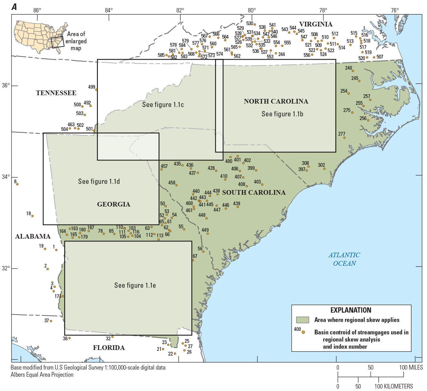
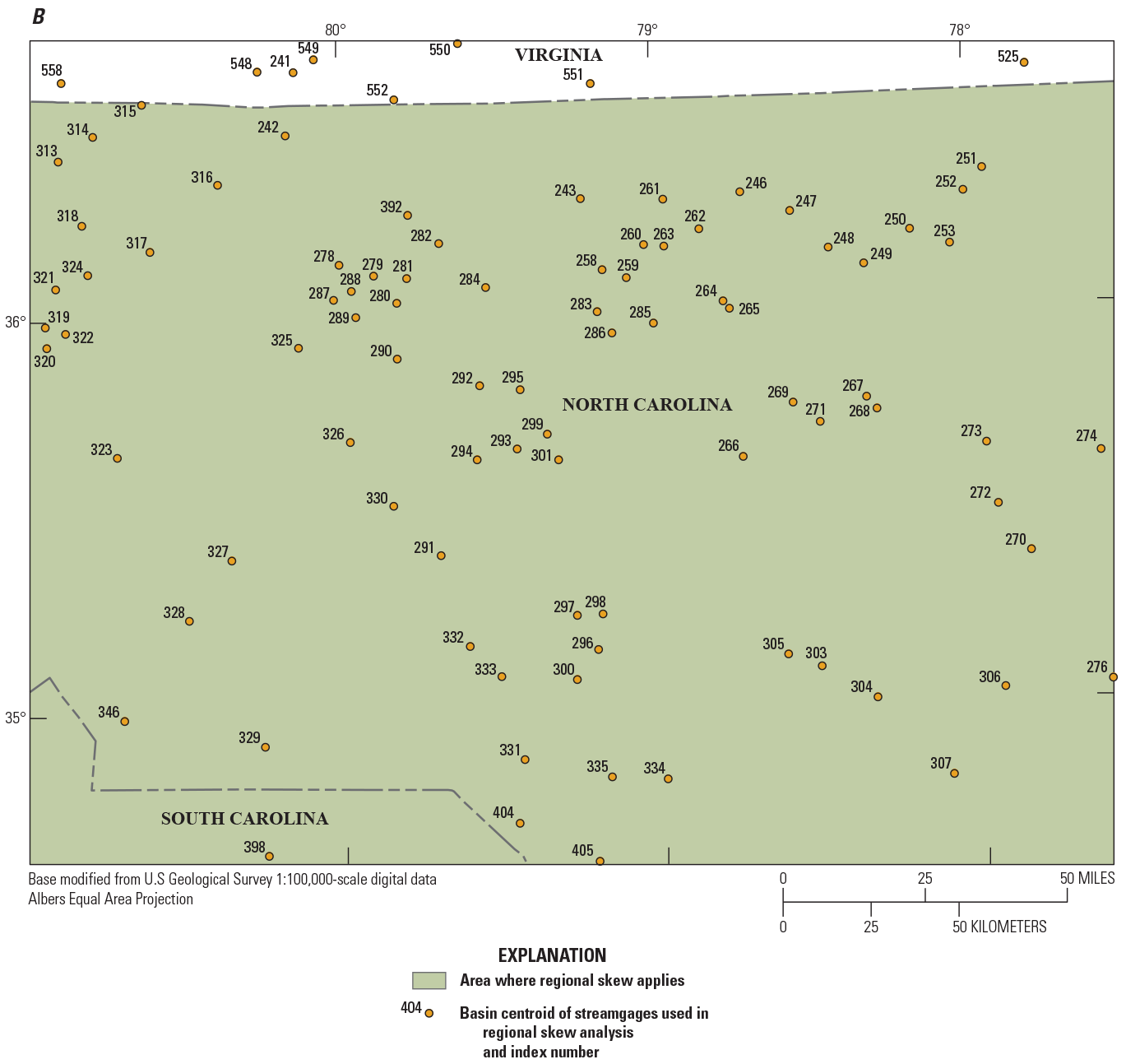
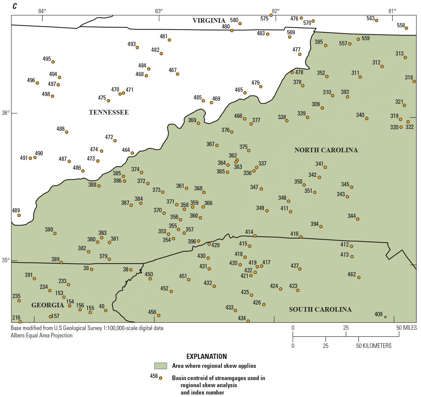
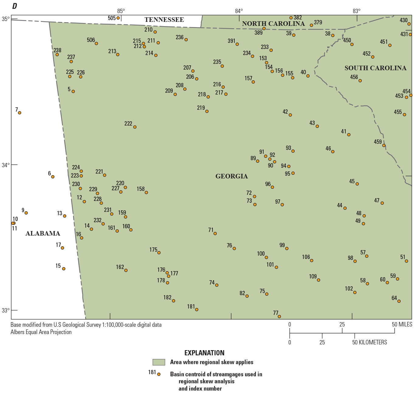
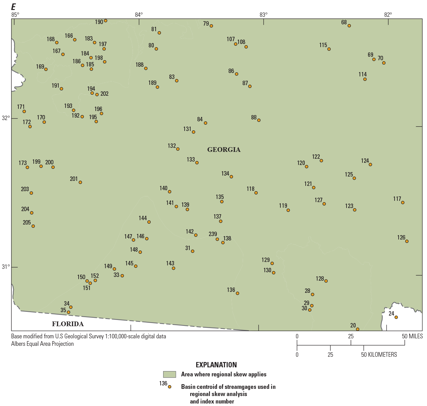
Map showing centroids of drainage basins of U.S. Geological Survey streamgages in Alabama, Florida, Georgia, North Carolina, South Carolina, Tennessee, and Virginia that were used for regional skew analysis.
Streamgage Skew
To estimate the streamgage skew, G, and its mean square error, MSEG, results of the EMA/MGBT analysis described earlier in this report were used (Cohn and others, 1997; Griffis and others, 2004). The EMA/MGBT provides a straightforward and efficient method for the incorporation of historic information and censored data, such as those from a crest-stage gage. Version 7.3 of USGS PeakFQ software (Veilleux and others, 2014, available at http://water.usgs.gov/software/PeakFQ/) incorporates EMA/MGBT, and was used to generate the streamgage skew (G) and its corresponding mean square error (MSEG), assuming a log-Pearson Type III distribution and generally applying MGBT for screening of PILFs (table 11 from Kolb and others, 2023); see “Estimation of Flood Magnitude and Frequency at Streamgages” section in this report for a more detailed description regarding EMA and MGBT.
Pseudo Record Length
Annual peak-flow records of streamgages often include historic information and censored data (for example, knowledge that the annual peak-flow at a crest-stage gage did not exceed the minimum recordable flow), which need to be accounted for when computing the precision of skew estimates. Whereas historic information and censored peaks are valuable information, they often provide less information than an equal number of years of gaged peaks (Stedinger and Cohn, 1986). The following calculations yield a pseudo record length, PRL, which appropriately accounts for all types of data available for a streamgage.
The PRL is defined in terms of the number of years of gaged record that would be required to yield the same mean square error of the skew, , as the combination of historic and gaged record available at a streamgage; thus, the PRL of the skew is a ratio of the MSE of the streamgage skew when only the gaged record is analyzed to the MSE of the streamgage skew when all of the data, including historic and censored data, are analyzed as and used in the following equation:
wherePRL
is the pseudo record length for the entire period of record at the streamgage, in years;
PS
is the number of gaged peaks in the record;
is the estimated MSE of the skew when only the gaged record is analyzed; and
is the estimated MSE of the skew when all the data, including historic and censored, are analyzed.
The PRL must be nonnegative, and the following conditions must also be met to ensure a valid approximation: (1) if the PRL is greater than PH (the length of the historic period), then PRL should be set to PH; and (2) if the PRL is less than PS, then the PRL is set to PS. This ensures that the PRL will not be larger than PH or less than PS.
The estimate of streamgage skew is sensitive to extreme flow events, and more accurate estimates can be obtained from longer streamflow records (England and others, 2019). Therefore, streamgages that have a PRL of less than 35 years are normally not used for regional skew analysis. The minimum PRL used in the study was 35 years, and the maximum was 169 years. Because of PRL values less than 35 years, 129 of 581 candidate streamgages were removed (table 11 from Kolb and others, 2023).
Redundant Streamgages
Redundancy results when the drainage basins of two streamgages are nested, meaning that one basin (representing the drainage area of one streamgage) is contained inside the other and the two basins are of similar size. Instead of representing two independent spatial observations that depict how drainage-basin characteristics are related to annual peak flows or skew, these two basins will have the same hydrologic response to a given storm event and, thus, represent only one spatial observation. When streamgages are redundant, a statistical analysis using both streamgages incorrectly represents the information in the regional dataset (Gruber and Stedinger, 2008). To determine if two streamgages are redundant and, thus, represent the same hydrologic conditions, two types of information are considered: (1) whether their basins are nested, and (2) the ratio of the drainage areas of the basins.
The standardized distance (SD) is used to determine the likelihood that the basins are nested. The SD between two basin centroids is defined as
whereDij
is the distance between centroids of basin i and basin j, in miles;
DAi
is the drainage area at site i, in square miles; and
DAj
is the drainage area at site j, in square miles.
The drainage-area ratio (DAR) is used to determine if two nested basins are sufficiently similar in size to conclude that these basins are, or are at least in large part, the same basin for the purposes of developing a regional hydrologic model. The DAR is defined as given by Veilleux (2009) as
whereDAR
is the maximum (max) of the two values in brackets;
DAi
is the drainage area at site i, in square miles; and
DAj
is the drainage area at site j, in square miles.
Two basins might be redundant if they are similar in size and their basins are nested. Previous studies suggest that streamgage pairs having SD less than or equal to 0.50 and DAR less than or equal to 5 were likely to be redundant for purposes of determining regional skew. If DAR is larger than 5, even if the streamgage pairs are nested, the streamgage pairs may reflect different hydrologic responses because storms of different sizes and durations will affect each streamgage basin differently. All possible combinations of streamgage pairs from 585 candidate streamgages were considered in the redundancy analysis. The 156 streamgage pairs identified as redundant were then investigated to determine if one streamgage of the pair was nested inside the other. For streamgage pairs that were nested, one streamgage from the pair was removed from the regional skew analysis. For redundancy, 88 streamgages were removed leaving 368 streamgages for use in the regional skew analysis (table 11 from Kolb and others, 2023).
Unbiasing the Streamgage Skew
For the 368 streamgages used in the regional skew analysis, the streamgage skews were unbiased using the correction factor developed by Tasker and Stedinger (1986) and applied by Reis and others (2005). The unbiased streamgage skew, computed using the PRL, is
whereis the unbiased streamgage skew estimate for streamgage i,
PRL,i
is the pseudo record length, in years, for streamgage i, as calculated in equation 1.2, and
Gi
is the biased estimate of streamgage skew for streamgage i from the flood‑frequency analysis.
The variance of the unbiased streamgage skew includes the correction factor developed by Tasker and Stedinger (1986):
where Var[Gi] is calculated using Griffis and Stedinger (2009) and given as whereEstimating the Mean Square Error of the Skew
There are various ways to estimate the MSEG. The approach used by EMA (see equation 55 in Cohn and others, 2001) generates a first order estimate of the MSEG, which should be an accurate estimate when interval data are present. Another option is to use the formula in equation 1.7 (the variance is equated to the MSE), using either the length of the gaged record or the length of the historic period (PH); however, this method does not account for censored data, and can lead to an inaccurate and underestimated MSEG. This issue has been addressed by using the PRL instead of PH; the PRL reflects the effect of the censored data and the number of gaged peaks. Thus, the MSE of the unbiased skew, computed using the formula from Griffis and Stedinger (2009), was used in the regional skew model because it is more stable and relatively independent of the streamgage skew. This methodology was used in previous regional skew studies (Eash and others, 2013; Southard and Veilleux, 2014).
Cross-Correlation Model
A critical step in a GLS analysis is estimation of the cross correlation of the skew estimates. Martins and Stedinger (2002) used Monte Carlo experiments to derive a relation between the cross correlation of the streamgage skew estimates at two streamgages, i and j, as a function of the cross correlation of concurrent annual peak flows, ρij:
whereis the cross correlation of concurrent annual peak flows for two streamgages, i and j;
κ
is a constant between 2.8 and 3.3; and
cfij
is a factor that accounts for the sample size difference between streamgages and their concurrent record length and is defined as follows:
CYij
is the pseudo record length of the period of concurrent record; and
PRL,i and PRL,j
are the pseudo record lengths corresponding to streamgages i and j, respectively (see equation 1.2).
After calculating the PRL for each streamgage considered in the study, the pseudo concurrent record length between pairs of streamgages can be calculated. Because of the use of censored and historic data, calculation of the effective concurrent record length is more complex than determining in which years the two streamgages both have recorded systematic flow peaks. First, the number of years of a historic period in common between the two streamgages are determined. Next, for the years in common, with beginning year YBij and ending year YEij, the following equation is used to calculate the concurrent years of record between site i and site j:
The computed pseudo concurrent record length depends on the years of historic period in common between the two streamgages, as well as the ratios of the PRL to the PH for each of the streamgages.
To relate the concurrent annual peak flows at two streamgages, ρij, to explanatory variables, a cross-correlation model using 59 streamgages with at least 85 years of concurrent gaged peak flows (zero flows not included) was considered. A logit model, termed the Fisher Z-Transformation (Z = log [(1+r)/ (1−r)]; fig. 1.2; Fisher, 1915), provided a convenient transformation of the sample correlations, rij, from the (−1, +1) range to the (−∞, +∞) range. The logit model used to estimate the cross correlations of concurrent annual peak flows at two streamgages that incorporated the distance between basin centroids, Dij, as the only explanatory variable, is
where where exp is the natural exponential function.An OLS regression analysis, based on 1,266 streamgage pairs from 59 sites, indicated that this model is as accurate as having 85 years of concurrent gaged peaks from which to calculate cross correlation. The fitted relation between the untransformed cross correlation and distance between basin centroids and points representing the 1,266 streamgage pairs is shown in figure 1.3. The cross-correlation model was used to estimate streamgage-to-streamgage cross correlation of concurrent annual peak flows for all streamgage pairs.
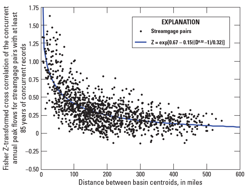
Graph showing relation between Fisher Z-transformed cross correlation of logarithms of annual peak flows and distance between basin centroids for streamgages in the southeastern United States regional skew study. Z, Fisher Z-transformation; exp, natural exponential function; D, distance between basin centroids, in miles.
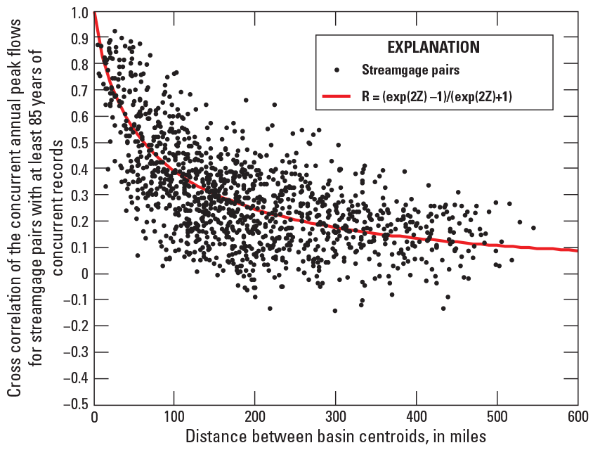
Graph showing relation between untransformed cross correlation of logarithms of annual peak flows and distance between basin centroids for streamgages in the southeastern United States regional skew study. R, sample correlations; exp, natural exponential function; Z, Fisher Z‑transformation.
Regional Skew Model for the Southeastern United States
In the B–WLS/B–GLS analysis of regional skew, 8 basin characteristics—drainage area, maximum elevation in the streamgage basin, perimeter of the streamgage basin, mean annual precipitation, channel slope, soil drainage index, percentage of the streamgage basin covered in impervious surface, and percentage of the streamgage basin covered in forest—were tested as explanatory variables (table 2 from Kolb and others, 2023). None of these basin characteristics was statistically significant or increased the pseudo R2; therefore, a constant model of regional skew (no covariates), 0.048, was selected for the southeastern United States (table 1.1).
Table 1.1.
Regional skew model for the southeastern United States.[Standard deviations are in parentheses; , model-error variance; ASEV, average sampling error variance; AVPnew, average variance of prediction for a new site; pseudo R2, fraction of the variability in the true skews explained by each model (Gruber and others, 2007)]
An appropriate regional skew model will have the smallest possible model-error variance,, and largest possible pseudo R2. A constant model does not explain variability in the true skews, so the pseudo R2, which describes the estimated fraction of the variability in the true skew from streamgage-to-streamgage determined with the model is zero (Gruber and others, 2007; Parrett and others, 2011). The posterior mean of the model-error variance, , is 0.088. The mean sampling error variance, ASEV, is 0.0036 and represents the mean error in the regional skew for the streamgages in the dataset. The average variance of prediction at a new streamgaging site (not part of the original number of streamgages considered), AVPnew, is 0.092, which corresponds to an effective record length of 73 years and is equivalent to the MSE used in Bulletin 17B to describe the precision of the generalized skew map.
Diagnostic Statistics for Bayesian Weighted Least Squares/Bayesian Generalized Least Squares Regression
To evaluate how well a regression model fits a regional hydrologic dataset, diagnostic statistics have been developed (Griffis, 2006; Gruber and others, 2007). A pseudo analysis of variance (pseudo ANOVA) was conducted for the constant model of regional skew in the southeastern United States (table 1.2). The pseudo ANOVA shows how much of the variation in the observed skews can be explained with application of the regional model, and how much of the variation in residuals can be attributed to model error and sampling error, respectively. Difficulties arise in determining these quantities. The model errors cannot be resolved because the values of the sampling errors, ηi, for each site, i, are not known. However, the total sampling error sum of squares can be described by its mean value, . Because there are n equations, the total variation because of the model error, δ, for a model with k parameters has a mean equal to ; thus, the residual variation attributed to the sampling error is , and the residual variation attributed to the model error is . This division of the variation in the observations is referred to as a pseudo ANOVA because the contributions of the three sources of error are estimated or developed, rather than being determined from the residuals and the model predictions, and also ignoring the effect of correlation among the sampling errors.
Table 1.2.
Pseudo analysis of variance (pseudo ANOVA) of the regional skew model for the southeastern United States.[Terms: k, number of estimated regression parameters not including the constant; n, number of streamgages used in regression; , model error variance of a constant model; , model error variance of a model with k regression parameters and a constant; NA, not applicable; , variance of the estimated sample skew at site i; EVR, error variance ratio; MBV*, misrepresentation of the beta variance; , regression constant from B–WLS analysis; GLS, Bayesian generalized least squares; WLS, Bayesian weighted least squares; WT, the transformation of W; Λ, covariance matrix; W, the (k × n) matrix of weights determined by B–WLS analysis; Wi = 1/Λii; pseudo R2, fraction of variability in the true skews explained by each model (Gruber and others, 2007); %, percent]
For a model with no explanatory variables (the constant model), the estimated model-error variance, , describes all of the anticipated variation in , where μ is the mean of the estimated streamgage sample skews; thus, the total expected sum of squares variation because of model error, δi, and because of sampling error, , in expectation should equal . The expected sum of squares attributed to a regional skew model with k parameters should then equal, because the sum of the model-error variance and the variance determined with the model must sum to . The constant model (table 1.1) has k = 0.
The ratio of the average-sampling error variance to the model-error variance is called the error variance ratio (EVR). The EVR is a diagnostic statistic used to evaluate if a simple OLS regression is sufficient or if a more sophisticated WLS or GLS analysis is appropriate. Generally, an EVR greater than 0.20 indicates that the sampling variance is not negligible when compared to the model-error variance. This result indicates the need for a WLS or GLS regression analysis. The EVR is calculated as
The EVR for the constant model is 1.5 (table 1.2). The sampling variability in the streamgage skew was larger than the error in the regional model; thus, neglecting sampling error in the streamgage skew in the OLS model might not have provided a statistically reliable analysis of the data. Given the variation of record lengths from streamgage to streamgage, it was important to use a WLS or GLS analysis to evaluate the final model accuracy and precision, rather than a simpler OLS analysis.
The misrepresentation of the beta variance (MBV*) is a diagnostic statistic used to determine whether a WLS regression is sufficient or a GLS regression is appropriate to determine the precision of the estimated regression parameters (Griffis, 2006; Veilleux, 2011). The MBV* describes the error produced by a WLS regression analysis in evaluating the precision of , which is the estimator of the constant . This description results because the covariance among the estimated streamgage skews, , generally has a greater effect on the precision of the constant term (Stedinger and Tasker, 1985, 1986). If the MBV* is substantially greater than 1, then a GLS error analysis should be applied. The MBV* is calculated as
MBV* was 6.4 for the constant model (table 1.2). This MBV* value is large, indicating that the cross correlation among the streamgage skew estimates affected the precision with which the regional skew could be estimated. If a WLS analysis were used to estimate the precision of the constant, the variance would be underestimated by a factor of 6.4; moreover, a WLS model would underestimate the variance of prediction, given that the sampling error in the constant term was sufficiently large to make an appreciable contribution to the average variance of prediction.
Leverage and Influence
Leverage and influence diagnostic statistics can be used to identify outlier observations and to effectively address lack of fit when estimating skew coefficients. Leverage identifies those streamgages in the analysis where the observed values have a large effect on the fitted (or predicted) values (Hoaglin and Welsch, 1978). Generally, leverage takes into consideration whether an observation, or explanatory variable, is unusual, and, thus, likely to have a large effect on the estimated regression coefficients and predictions. Unlike leverage, which highlights points with the capacity or potential to affect the fit of the regression, influence attempts to describe those points with an unusual effect on the regression analysis (Belsley and others, 1980; Cook and Weisberg, 1982; Tasker and Stedinger, 1989). An influential observation is one with an unusually large residual that has a disproportionate effect on the fitted regression. Influential observations often have high leverage. Detailed descriptions of the equations used to determine leverage and influence for a B–WLS/B–GLS analysis can be found in Veilleux (2011) and Veilleux and others (2011).
No streamgages in the regional skew analysis had high leverage (greater than 0.005435). The differences in leverage values for the constant model reflect the variation in record lengths among all streamgages considered. Thirty streamgages had high influence (Cook’s D, a measure of the difference between the model with all observations included and the model with the observation in question removed, greater than 0.01087) and, thus, had an unusual effect on the fitted regression (table 1.3).
Table 1.3.
Streamgages used in regional skew model of the southeastern United States with high influence (Cook's D greater than 0.01087) on the fitted regression.[USGS, U.S. Geological Survey; B–WLS/B–GLS, Bayesian weighted least squares/Bayesian generalized least squares]
| Map index number (see fig. 1.1) | USGS streamgage number | Leverage (base 10 log units) | Cook's D (base 10 log units) | Residual, B–WLS/B–GLS analysis (base 10 log units) |
|---|---|---|---|---|
| 92 | 02217500 | 0.00348 | 0.04609 | −1.237 |
| 215 | 02387000 | 0.00386 | 0.04389 | −1.028 |
| 352 | 03161000 | 0.00330 | 0.04002 | 1.247 |
| 276 | 02092500 | 0.00290 | 0.03032 | 1.363 |
| 49 | 02193500 | 0.00274 | 0.02942 | −1.456 |
| 332 | 02133500 | 0.00313 | 0.02690 | 1.125 |
| 458 | 02196000 | 0.00320 | 0.02504 | −1.048 |
| 76 | 02213000 | 0.00375 | 0.02233 | −0.762 |
| 251 | 02082950 | 0.00269 | 0.02052 | 1.262 |
| 357 | 03443000 | 0.00351 | 0.01955 | 0.797 |
| 106 | 02223500 | 0.00375 | 0.01881 | −0.699 |
| 54 | 02198000 | 0.00318 | 0.01808 | 0.907 |
| 189 | 02349900 | 0.00290 | 0.01713 | −1.014 |
| 480 | 03487550 | 0.00255 | 0.01594 | 1.202 |
| 12 | 02412000 | 0.00328 | 0.01582 | 0.802 |
| 178 | 02346180 | 0.00329 | 0.01557 | −0.792 |
| 543 | 02064000 | 0.00311 | 0.01471 | 0.842 |
| 99 | 02220900 | 0.00278 | 0.01470 | −1.000 |
| 51 | 02197520 | 0.00370 | 0.01452 | 0.635 |
| 304 | 02106500 | 0.00290 | 0.01413 | 0.929 |
| 432 | 02163500 | 0.00313 | 0.01391 | −0.801 |
| 277 | 02093000 | 0.00261 | 0.01297 | 1.057 |
| 136 | 02317600 | 0.00269 | 0.01297 | −1.004 |
| 567 | 03175500 | 0.00348 | 0.01262 | −0.650 |
| 205 | 02357000 | 0.00313 | 0.01259 | −0.774 |
| 188 | 02349695 | 0.00217 | 0.01258 | −1.382 |
| 365 | 03451000 | 0.00344 | 0.01232 | 0.655 |
| 52 | 02197600 | 0.00237 | 0.01207 | 1.174 |
| 240 | 02053200 | 0.00274 | 0.01190 | 0.936 |
| 84 | 02215245 | 0.00252 | 0.01174 | −1.049 |
Monte Carlo Analysis of Spatial Patterns in Skew
A graphical assessment of the B–WLS/B–GLS model of regional skew for the southeastern United States was conducted to provide information on the geographic patterns in skew. A contour map of unbiased skew, created using locally weighted scatterplot smoothing (LOWESS), indicates a large area of negative skews in Georgia and clusters of positive skews in South Carolina and North Carolina (fig. 1.4).
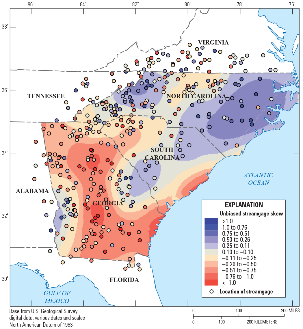
Contour shade map showing unbiased streamgage skews for 368 streamgages used in the regional skew analysis of the southeastern United States.
Monte Carlo simulations were used to determine whether the geographic patterns observed in the unbiased streamgage skews are evidence of model misspecification or an artifact of random-sampling variability that is possibly confounded by the covariance structure of the errors. The Monte Carlo simulations were generated from a multivariate normal distribution with a mean equal to the constant from the regional skew model and a covariance matrix identical to the covariance matrix used in the regional skew model. The constant model of regional skew in the study area is
where ε represents the total error and where N signifies a normal distribution of the total error in the regional skew model.The Var(ε) can be described as
whereεT
is the transformation of ε;
is the (n × n) B–GLS covariance matrix;
is the B–GLS variance of the underlying model‑error δ;
I
is an (n × n) identity matrix; and
is the full (n × n) covariance matrix of the sampling errors for each streamgage (n).
The covariance matrix of the sampling errors is made up of the sampling variances of the unbiased streamgage skew () and the covariances of the skew estimators (). The off-diagonal values of the covariance matrix are determined by the cross correlation of concurrent gaged annual peak flows and the cf factor (see equation 3 from Martins and Stedinger, 2002). The model-error variance for the constant model is 0.088 (table 1.1) and was used in the Monte Carlo simulations. The covariance matrix used in the Monte Carlo simulations is the same as that used in the B–WLS/B–GLS regression analysis.
The results of the Monte Carlo simulations are depicted graphically in 20 iterations (fig. 1.5A–T) of the expected patterns in the unbiased streamgage skews if they were normally distributed with a mean equal to 0.048 and a covariance matrix given by equation 1.16. The Monte Carlo simulations reveal no structure in the pattern of the unbiased streamgage skews that is consistent with the observed pattern of the unbiased streamgage skews (fig. 1.4). Therefore, it is reasonable to conclude that, despite the geographic patterns observed in the unbiased streamgage skews, there is little evidence of a lack of fit of these skews.
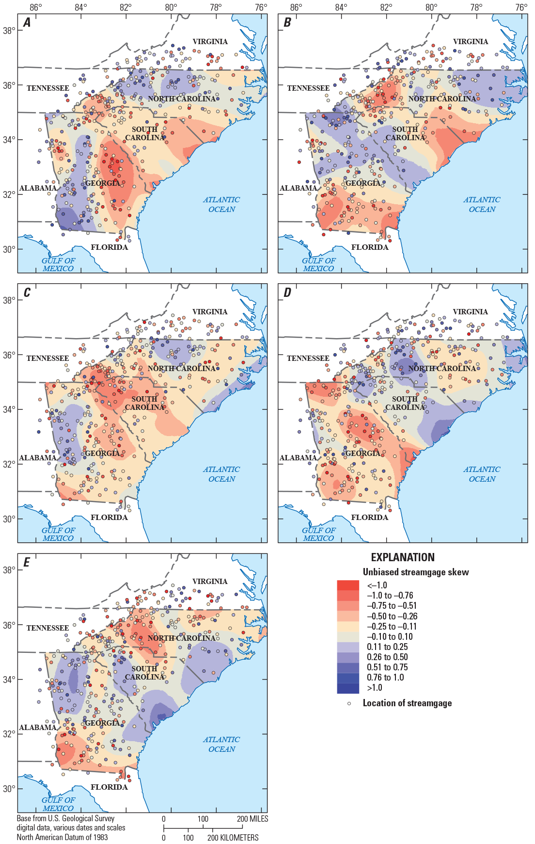
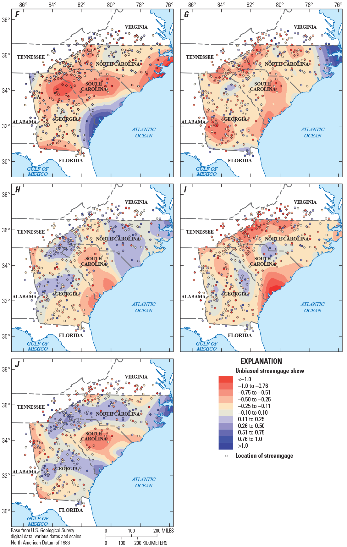
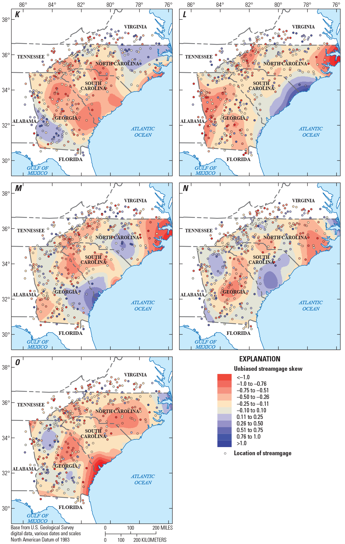
Contour shade maps showing the results of 20 Monte Carlo simulations (A–T) of unbiased skew at 368 streamgages in the southeastern United States that were used in the regional skew analysis. Simulations are normally distributed to the constant skew model and covariance matrix.
References Cited
England, J.F., Jr., Cohn, T.A., Faber, B.A., Stedinger, J.R., Thomas, W.O., Jr., Veilleux, A.G., Kiang, J.E., and Mason, R.R., Jr., 2019, Guidelines for determining flood flow frequency—Bulletin 17C (ver. 1.1, May 2019): U.S. Geological Survey Techniques and Methods, book 4, chap. B5, 148 p. [Also available at https://doi.org/10.3133/tm4B5.]
Gruber, A.M., Reis, D.S., Jr., and Stedinger, J.R., 2007, Models of regional skew based on Bayesian GLS regression, in Kabbes, K.C., ed., Restoring our natural habitat—Proceedings of the World Environmental and Water Resources Congress, Tampa, Fla., May 15–18, 2007: Reston, Va., American Society of Civil Engineers, 10 p.
Gruber, A.M., and Stedinger, J.R., 2008, Models of LP3 regional skew, data selection and Bayesian GLS regression, in Babcock, R.W., Jr., and Walton, R., eds., Ahupua’a—Proceedings of the World Environmental and Water Resources Congress, Honolulu, Hawai’i, May 12–16, 2008: Reston, Va., American Society of Civil Engineers, 10 p.
Kolb, K.R., Musser, J.W., Feaster, T.D, Gotvald, A.J., and Weaver, J.C., 2023, Magnitude and frequency of floods for rural streams in Georgia, South Carolina, and North Carolina, 2017—Data: U.S. Geological Survey data release, https://doi.org/10.5066/P9TSBPFS.
Lamontagne, J.R., Stedinger, J.R., Berenbrock, C., Veilleux, A.G., Ferris, J.C., and Knifong, D.L., 2012, Development of regional skews for selected flood durations for the Central Valley Region, California, based on data through water year 2008: U.S. Geological Survey Scientific Investigations Report 2012–5130, 60 p.
Parrett, C., Veilleux, A., Stedinger, J.R., Barth, N.A., Knifong, D.L., and Ferris, J.C., 2011, Regional skew for California, and flood frequency for selected sites in the Sacramento–San Joaquin River Basin, based on data through water year 2006: U.S. Geological Survey Scientific Investigations Report 2010–5260, 94 p.
Southard, R.E., and Veilleux, A.G., 2014, Methods for estimating annual exceedance-probability discharges and largest recorded floods for unregulated streams in rural Missouri: U.S. Geological Survey Scientific Investigations Report 2014–5165, 39 p., accessed April 30, 2015, at http://dx.doi.org/10.3133/sir20145165.
U.S. Geological Survey, 2019, Peak Streamflow for the Nation: U.S. Geological Survey National Water Information System database, accessed June 7, 2019, at https://nwis.waterdata.usgs.gov/usa/nwis/peak.
Veilleux, A.G.; Cohn, T.A.; Flynn, K.M.; Mason, R.R., Jr.; and Hummel, P.R., 2014, Estimating magnitude and frequency of floods using the PeakFQ 7.0 program: U.S. Geological Survey Fact Sheet 2013–3108, 2 p., accessed October 22, 2015, at http://dx.doi.org/10.3133/fs20133108.
Veilleux, A.G., Stedinger, J.R., and Eash, D.A., 2012, Bayesian WLS/GLS regression for regional skewness analysis for regions with large crest stage gage networks, in Loucks, E.D., ed., Crossing boundaries—Proceedings of the World Environmental and Water Resources Congress, Albuquerque, N. Mex., May 20–24, 2012: Reston, Va., American Society of Civil Engineers, p. 2253–2263.
Veilleux, A.G., Stedinger, J.R., and Lamontagne, J.R., 2011, Bayesian WLS/GLS regression for regional skewness analysis for regions with large cross-correlations among flood flows, in Beighley, R.E., II, and Killgore, M.W., eds., Bearing knowledge for sustainability—Proceedings of the World Environmental and Water Resources Congress, Palm Springs, Calif., May 22–26, 2011: Reston, Va., American Society of Civil Engineers, p. 3103–3112.
Conversion Factors
U.S. customary units to International System of Units
Temperature in degrees Celsius (°C) may be converted to degrees Fahrenheit (°F) as follows: °F = (1.8 × °C) + 32.
Temperature in degrees Fahrenheit (°F) may be converted to degrees Celsius (°C) as follows: °C = (°F – 32) / 1.8.
Datum
Vertical coordinate information is referenced to the North American Vertical Datum of 1988 (NAVD 88).
Horizontal coordinate information is referenced to the North American Datum of 1983 (NAD 83).
Altitude, as used in this report, refers to distance above the vertical datum.
Abbreviations
AEP
annual exceedance probability
APS
all possible subsets
AVP
average variance of prediction
DEM
digital elevation model
EMA
expected moments algorithm
EPA
U.S. Environmental Protection Agency
FEMA
Federal Emergency Management Agency
GIS
geographic information system
GLS
generalized least squares
HR
hydrologic region
lidar
light detection and ranging
LPIII
log-Pearson Type III
MGBT
multiple Grubbs Beck test
MSE
mean square error
MOVE.1
Maintenance of Variance Extension, Type 1
MOVE.2
Maintenance of Variance Extension, Type 2
NWIS
National Water Information System
OLS
ordinary least squares
PILF
potentially influential low flow
QA/QC
quality assurance and quality control
SMC
single-mass curve
USGS
U.S. Geological Survey
VIF
variance inflation factor
WLS
weighted least squares
WREG
weighted-multiple-linear regression
Disclaimers
Any use of trade, firm, or product names is for descriptive purposes only and does not imply endorsement by the U.S. Government.
Although this information product, for the most part, is in the public domain, it also may contain copyrighted materials as noted in the text. Permission to reproduce copyrighted items must be secured from the copyright owner.
Suggested Citation
Feaster, T.D., Gotvald, A.J., Musser, J.W., Weaver, J.C., Kolb, K.R., Veilleux, A.G., and Wagner, D.M., 2023, Magnitude and frequency of floods for rural streams in Georgia, South Carolina, and North Carolina, 2017—Results: U.S. Geological Survey Scientific Investigations Report 2023–5006, 75 p., https://doi.org/10.3133/sir20235006.
ISSN: 2328-0328 (online)
Study Area
| Publication type | Report |
|---|---|
| Publication Subtype | USGS Numbered Series |
| Title | Magnitude and frequency of floods for rural streams in Georgia, South Carolina, and North Carolina, 2017—Results |
| Series title | Scientific Investigations Report |
| Series number | 2023-5006 |
| DOI | 10.3133/sir20235006 |
| Publication Date | April 28, 2023 |
| Year Published | 2023 |
| Language | English |
| Publisher | U.S. Geological Survey |
| Publisher location | Reston, VA |
| Contributing office(s) | Georgia Water Science Center, South Atlantic Water Science Center |
| Description | Report: ix, 75 p.; 2 Data Releases |
| Country | United States |
| State | Georgia, North Carolina, South Carolina |
| Online Only (Y/N) | Y |
| Additional Online Files (Y/N) | N |