

Hydrologic Framework and Characterization of the Little Colorado River Alluvial Aquifer near Leupp, Arizona
Links
- Document: Report (16 MB pdf) , HTML , XML
- Appendixes:
- Appendix 1 (30 KB xlsx) - Water-chemistry sample results from monitoring wells, Little Colorado River alluvial aquifer, northeastern Arizona
- Appendix 2 (30 KB xlsx) - Major ion chemistry results of water samples collected from springs and wells in the Moenkopi Formation in Arizona
- Data Releases:
- NGMDB Index Page: National Geologic Map Database Index Page (html)
- Download citation as: RIS | Dublin Core
Acknowledgments
The authors extend their appreciation to the Navajo Nation Council, Navajo Nation Department of Water Resources Water Management Branch, and the Navajo Nation Chapters of Leupp and Birdsprings for their cooperation and support of this study.
Abstract
The Little Colorado River alluvial aquifer near Leupp, Arizona, was investigated as a possible source of irrigation water for the Leupp and Birdsprings Chapters of the Navajo Nation. The physical, chemical, and hydraulic characteristics of the alluvial aquifer were studied using geophysical surveys, installation of observation wells, water-level measurements, chemical analyses, groundwater pumping simulations, and review of previous investigations. Geophysical surveys and well borings revealed that the aquifer ranges in thickness from near 0 feet around its periphery to about 100 feet in its thickest parts. Water levels were monitored in nine alluvial wells within the study area and compared with earlier measurements collected in 1998 and 1999. Comparison of those earlier water levels with water levels collected as part of this study showed a decline of between about 5 and 12 feet has occurred in the last 23 years. The water chemistry of the aquifer was analyzed for salinity hazard, sodium-adsorption hazard, and specific-ion toxicity. The sodium-adsorption hazard and specific-ion toxicity of alluvial aquifer water were found to be low. However, the salinity hazard was high enough in most areas that it could negatively affect salt-sensitive crops. Well-field pumping scenarios conducted for this study demonstrated that using groundwater from the alluvial aquifer for irrigated agriculture is theoretically possible but may be economically challenging owing to the hydraulic properties of the aquifer.
Introduction
The Navajo Nation covers more than 27,000 square miles (mi2) in parts of Arizona, Utah, and New Mexico. Water is a limiting resource on the Nation owing in large part to the arid climate of the region. The inaccessibility of water for crop irrigation across most of the Nation limits the opportunity for economically sustainable agriculture. To identify potential new irrigation resources, the Navajo Nation along with the Chapters of Leupp and Birdsprings collaborated with the U.S. Geological Survey (USGS) to study the feasibility of using groundwater from the Little Colorado River alluvial aquifer for irrigated agriculture in an area where Corn Creek Wash enters the Little Colorado River near Leupp, Ariz. (fig. 1). The Little Colorado River alluvial aquifer is referred to herein as the “alluvial aquifer.”
The alluvial aquifer consists of the saturated portion of channel and floodplain sediments (alluvium) deposited by the Little Colorado River and its tributary streams such as Corn Creek Wash. Within the study area, the base of the alluvial aquifer is delineated by bedrock of the Moenkopi or Chinle Formations. The Little Colorado River is the principal source of recharge for the alluvial aquifer in the study area (Johnson, 1999a, c). The river is an ephemeral stream through the study area flowing only in response to precipitation and snowmelt runoff. Most flow through the study area occurs either when snow melts on the Mogollon Rim to the south during the winter and early spring, or during the summer monsoon season when thunderstorms are common in the region.
The community of Leupp was originally located on the floodplain of the Little Colorado River approximately 2.5 miles (mi) southeast of its current location. The original townsite is known locally as “Old Leupp.” In the past, water from the alluvial aquifer was used to supply water for the school at Old Leupp. Also, one irrigation well that is no longer in use supplied a small farm about 3 mi east of Old Leupp. Currently the alluvial aquifer is largely unused in the study area except for a few wells used to produce water for livestock.
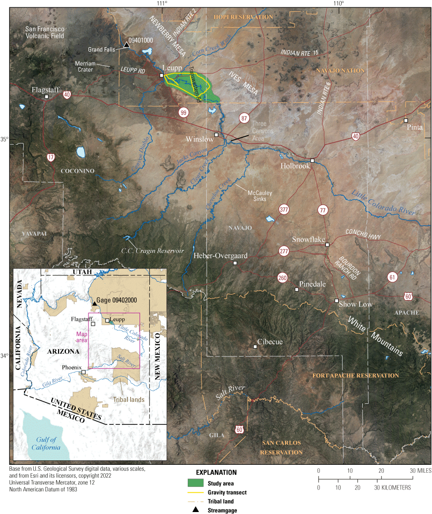
Map showing location of the Little Colorado River alluvial aquifer study area, northeastern Arizona.
Purpose and Scope
This report describes the physical, chemical, and hydraulic characteristics of the alluvial aquifer near Leupp, Ariz., based on geophysical surveys, water-level measurements, chemical analyses, and previous investigations. The report also discusses the suitability of alluvial aquifer water for irrigating crops and describes the results of hypothetical single and multiple well pumping scenarios to assess how the aquifer would be affected by irrigation pumping.
Previous Investigations
This study builds on a comprehensive investigation conducted by the Navajo Nation Department of Water Resources Water Management Branch in cooperation with the Bureau of Reclamation (Reclamation) and the Bureau of Indian Affairs (BIA). The results of that investigation are published in a four-volume report (Johnson 1999a–d). The purpose of that study was to assess the feasibility of using water from the alluvial aquifer to supplement a proposed project called the Three Canyons Water Supply Project.
The purpose of the Three Canyons Water Supply Project was for the Nation to obtain an annual yield of 6,000 acre-feet (acre-ft) of ground- and surface-water from Clear Creek, Chevelon Creek, and Jacks Canyon (informally known as the Three Canyons area), south of the Nation, and then potentially make available 3,000 acre-ft of water from C.C. Cragin (formerly Blue Ridge) Reservoir in the Clear Creek watershed to non-Indian communities of northern Gila County (Navajo Nation Department of Water Resources, 2000). The 6,000 acre-ft of water from the Three Canyons area would be conveyed to the Leupp area where the Nation might increase the total available supply through conjunctive use of alluvial aquifer water (Johnson, 1999a). The Three Canyons Water Supply Project was subsequently postponed as a result of “changing circumstances” (Navajo Nation Department of Water Resources, 2011).
Volume I of the report (Johnson, 1999a) discusses the hydrogeology, hydraulic properties, and water budget of the alluvial aquifer. Volume II (Johnson, 1999b) describes the water chemistry of the aquifer. Volume III (Johnson, 1999c) summarizes the hydrogeology, stratigraphy, and water-bearing characteristics of the alluvial aquifer and synthesizes them into a conceptual hydrogeologic model of the aquifer. Volume IV (Johnson, 1999d) describes a plan for further characterization activities for the alluvial aquifer. Finally, a related report (Reclamation, 1999) describes a preliminary numerical groundwater model created for the aquifer and provides results of simulations done using the model.
Another extensive investigation conducted on the alluvial aquifer was done by Dohm (1995). He created a water budget for the aquifer and identified areas with favorable hydrogeologic conditions for future groundwater development. In addition, he discusses the potential for using alluvial aquifer water for crop irrigation.
Cooley and others (1969) provided an extensive overview of regional hydrogeology on the Navajo and Hopi Nations but relatively little information on alluvial aquifers. Mann (1976) described the availability, chemical quality, and use of groundwater in southern Navajo County, Ariz. A geologic map of the Leupp quadrangle was done by Irwin and others (1962). Ulrich and others (1984) compiled a map showing geology, structure, and uranium deposits for the Flagstaff 1° × 2° quadrangle, Arizona, and Billingsley and others (2013) created a geologic map of the Winslow 30′ × 60′ quadrangle, Coconino and Navajo Counties, northern Arizona.
Description of the Study Area
For practical reasons, the bounds of the study area used in this investigation are the same bounds used by Johnson (1999a–d). The study area encompasses about a 20-mi length of floodplain along the Little Colorado River between Leupp, Ariz., and the southern boundary of the Navajo Nation (fig. 1). Within this larger study area, the current investigation also had a focused area of study near the confluence of Corn Creek Wash and the Little Colorado River where irrigated agriculture has been proposed.
The floodplain of the Little Colorado River in the study area is broad, about 2 to 4 mi across, and covered with Tamarix spp. (tamarisk) stands of varying densities. In places, the mapped alluvium is greater than 4 mi across, but most of the sediments in these areas are likely derived from tributary washes rather than the Little Colorado River itself. The elevation of the Little Colorado River channel is about 4,800 feet (ft) above mean sea level at the southeast end of the study area where the river crosses into the Navajo Nation, and about 4,700 ft above mean sea level about 20 mi downstream at the northwest end of the study area, near the present-day town of Leupp. Outside of the Old Leupp townsite there are very few residences in the study area. The only commercial activity of note is livestock grazing. With minor exceptions, all roads in the study area are dirt, although particularly in the Old Leupp area they are well built and maintained.
Physiography
The study area is located within the Colorado Plateaus physiographic province (Raisz, 1972) and defined by the floodplain of the Little Colorado River, beginning where it crosses onto Navajo Nation lands north of Winslow, Ariz., and ending about 20 mi to the northwest, just east of the town of Leupp, Ariz. (fig. 1). Within the study area, the Little Colorado River occupies the lowland between the San Francisco Volcanic Field and Newberry and Ives Mesas. The geologic units in this area dip around 1 degree to the northeast (Ulrich and others, 1984). The Little Colorado River runs approximately perpendicular to this dip so that it roughly parallels the contact between the Triassic Moenkopi and Chinle Formations.
An important geomorphic event with large implications for the alluvial aquifer occurred downstream of the study area during the late Pleistocene. Around 20,000 years ago, a basalt lava flow erupted from vents near Merriam Crater and flowed north towards the narrow canyon containing the Little Colorado River (Duffield and others, 2006). About 18 mi downstream of the study area, the lava flow completely filled and crossed a 200-ft-deep section of the canyon, forming a natural dam (fig. 2). Lava continued to flow in the channel of the Little Colorado River for about 15 mi downstream of the dam (Moore and Wolf, 1987). Remnants of this flow are visible near the dam, but farther downstream this “intracanyon flow” forms the bed of the river and is less visible (Duffield and others, 2006). It is likely that lava flowed upstream of the dam for some distance as well, but how far upstream is unclear because thick alluvial sediments now cover this area. A lake (possibly as deep as 200 ft) would have formed in the canyon above the dam, although it would eventually be completely filled with sediment transported by the Little Colorado River and tributary drainages.
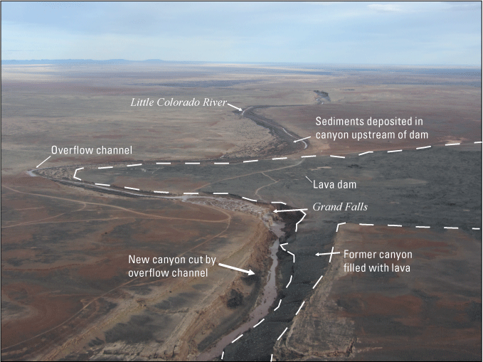
Oblique aerial photograph looking southeast at Pleistocene lava dam crossing canyon containing the Little Colorado River, Arizona. Dashed line outlines lava flow. Overflow channel around dam, the Grand Falls, segment of former canyon filled with lava, new canyon cut by overflow around dam, and sediments deposited in canyon upstream of dam are visible. Photograph by Jon Mason, U.S. Geological Survey, March 28, 2020.
It is unclear if the lake extended upstream into the study area. The upstream extent of the lake would have depended on the elevation of the bedrock upstream of the dam, and how much alluvial fill was already over the bedrock at the time. The current elevation of the lava flow where it crosses the canyon is about 4,650 ft. The lowest published elevation of the bedrock in the study area is about 4,560 ft (Johnson, 1999a). Johnson (1999a) identified sediments in some well borings that were interpreted as being the result of the damming of the Little Colorado River, noting that the sediments had a similar lithology to sediments mapped as Alluvial Unit M by Ulrich and others (1984). Alluvial Unit M is described by Ulrich and others (1984) as “valley fill resulted from damming of the Little Colorado River by basalt flow (Qbm) from Merriam Crater area.” It is unclear if the sediments described from well borings by Johnson (1999a) are definitely reservoir sediments because some of them are present at elevations higher than the top elevation of the lava dam. Other feasible interpretations for the origin of these sediments include the possibility they are overbank alluvial deposits of the Little Colorado River or weathered Chinle Formation. Even if the lake did not extend all the way to the study area, the dam would have lowered the gradient of the river enough to result in aggradation of sediment through the study area, which would have increased the thickness of the present-day alluvial aquifer. The sediments described by Johnson (1999a) are still important regarding the alluvial aquifer because they form the base of the aquifer in some areas.
A new river channel was eventually established around the dam forming the Grand Falls (fig. 2). The floodplain of the Little Colorado River is relatively wide in the study area compared to the incised channel that exists downstream of the lava dam. The study area floodplain probably was not this wide before the dam lowered the stream gradient. Based on geophysical data as well as borehole logs, it seems likely that a buried canyon or paleovalley exists in the bedrock through much or all of the study area similar in character to what currently exists below the lava dam.
The Little Colorado River through the study area is ephemeral with a floodplain covered with tamarisk stands of varying densities. From an aerial perspective, curved rows of tamarisk thickets are commonly visible (fig. 3), probably representing seed lines deposited during floods. Tamarisk can also reproduce vegetatively from stems torn from mature plants and buried by sediment during floods (Howard and Horton, 1965).
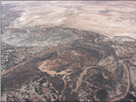
Aerial photograph showing curved rows of tamarisk stands along the Little Colorado River, Arizona, approximately 1 mile west of site 20. Photograph by Jon Mason, U.S. Geological Survey, March 28, 2020.
A series of ephemeral streams drain the Black Mesa area to the north, converging into a single channel (Corn Creek Wash) which enters the Little Colorado River from the northeast near the top of the study area. Another large ephemeral stream, Canyon Diablo Wash, enters the Little Colorado River from the southwest nearly opposite Corn Creek Wash. In addition, numerous poorly developed ephemeral drainages enter the Little Colorado River from both sides throughout the study area, and man-made dikes direct overland flow towards the Little Colorado River and to earthen stock tanks. To the south and west of the study area, elevation increases gradually up to the southern edge of the Colorado Plateau, known as the Mogollon Rim. Clear and Chevelon Creeks are two major tributaries of the Little Colorado River that drain parts of the Mogollon Rim. Springs issuing from the Coconino (C) aquifer (Bills and others, 2007) in these streams near their confluence with the Little Colorado River allow for a short reach of meager perennial flow above the study area. Both Clear and Chevelon Creeks form canyons near their confluence with the Little Colorado River. The Three Canyons area is where these two creeks enter the Little Colorado River in conjunction with a nearby third canyon, named Jacks Canyon (fig. 1).
Climate
The Köppen climate type that characterizes the study area is Cold Desert (BWk) (PRISM Climate Group, 2020). A weather station existed in Old Leupp from 1914 to 1981 at an elevation of about 4,700 ft above mean sea level (Western Regional Climate Center, 2022a; table 1). The coldest month on average was January with an average minimum temperature of 16.3 degrees Fahrenheit (°F) and an average maximum temperature of 45.8 °F (table 1). The warmest month was July with an average high temperature of 95.2 °F and an average low temperature of 58.8 °F. The annual mean temperature in Old Leupp from 1914 to 1981 was 53.8 °F, the highest recorded temperature was 110 °F, and the lowest temperature was −19 °F (Western Regional Climate Center, 2022b). Annual precipitation averaged 6.50 inches (in.). The months with the least average rainfall were May (0.23 in.) and June (0.29 in.) (Western Regional Climate Center, 2022a). Snow fell at least once at some point in the record in each of 6 months (October through March), with an annual average total of about 6 in. There were 25 in. of snow in the snowiest winter (1967–68), whereas in numerous years no snow fell (Western Regional Climate Center, 2022c).
Table 1.
Monthly and annual temperature, precipitation, and snowfall averages for National Weather Service Cooperative Stations Leupp, Arizona (024872) and Winslow Municipal Airport, Arizona (029439).[Data from Western Regional Climate Center (2022a), National Oceanic and Atmospheric Administration (2020). Leupp station averages are based on records collected 10/1/1914–4/30/1981. Winslow data are 1991–2020 climate normal. max., maximum; min. minimum; °F, degrees Fahrenheit; in., inches.]
The Winslow weather station at the municipal airport, 10 mi southeast of the southeast end of the study area, is 4,895 ft above sea level (National Oceanic and Atmospheric Administration, 2020). The meteorological record available from the National Centers for Environmental Information runs from 1893 to 2020. For the most recent 30-year period (1991 to 2020), the coldest month on average was December with an average minimum temperature of 21.7 °F and an average maximum temperature of 48.7 °F (table 1). The warmest month was July with an average high temperature of 94.6 °F and an average low temperature of 63.7 °F. The annual mean temperature in Winslow from 1991 to 2020 was 56.7 °F. The highest temperature ever recorded in Winslow was 109 °F and the lowest temperature ever was −19 °F (Western Regional Climate Center, 2022d). Annual precipitation from 1991 to 2020 averaged 6.52 in. with 3.06 in. of that total coming during the North American Monsoon, from June to September. The months with the least average rainfall were April (0.25 in.), May (0.30 in.), and June (0.14 in.). The remaining months of the year precipitation averaged around 0.5 in. per month (National Oceanic and Atmospheric Administration, 2020). Snowfall data are missing for Winslow beginning in 1996. Before that, 1 in. or more of snow has been recorded at some point in the record in 7 of 12 months (October through April). Mean annual snowfall over the entire period of record is about 11 in. The snowiest winter (1967–68) saw 43 in., and the least-snowy winter (1942–43) recorded no snow at all (Western Regional Climate Center, 2022e).
Hydrology and Hydrogeology
Based on the lithology described from borehole logs by Johnson (1999a), the alluvial sediments in the study area are composed of interbedded layers containing mixtures of silt, clay, sand, and fine gravel. Sands and silty sands are the most common lithology reported by Johnson (1999a). Based on three aquifer tests, Johnson (1999a) estimated the specific yield of the alluvial aquifer to be 0.19. Theoretically (ignoring lateral inflow and areal recharge) this means that under a 1-acre area, about 5 vertical feet of the aquifer would need to be dewatered for every acre-foot of water produced from that area.
The primary bedrock units in the study area are the Triassic Moenkopi and Chinle Formations. At the surface and in boreholes, the Moenkopi Formation is a dark reddish-brown mudstone, sandstone, or siltstone. Owing to the northeastward dip of the sedimentary units in the study area, the Moenkopi Formation is exposed at the western edge of the study area and is present in the subsurface throughout the remainder of the study area. Overlying the Moenkopi Formation, the Shinarump and Petrified Forest members of the Chinle Formation are present at the land surface in parts of the southern study area and in some northern areas east of the Little Colorado River.
Billingsley and others (2013) described the Shinarump Member of the Chinle Formation as “white, light-brown, and yellowish-pink, cliff-forming, coarse-grained sandstone and conglomeratic sandstone” with a thickness ranging from 60 to 80 ft. They described the Petrified Forest Member as “purple, blue, light-red, red-purple, and gray-blue, slope-forming mudstone and siltstone, interbedded with white to yellow-white, coarse-grained, lenticular sandstone” with a total thickness ranging from 350 to 430 ft.
Alluvium appears to rest unconformably on the Moenkopi Formation across much of the study area based on borehole logs from Johnson (1999a) and on the geologic maps of Ulrich and others (1984) and Billingsley and others (2013). Some alluvium in the eastern and southern parts of the study area could overlie the Chinle Formation. Although a few wells in Arizona produce water from the Moenkopi and Chinle Formations (presumably from sandstones layers), they are generally considered aquitards in the state because they usually contain abundant fine-grained beds. The Moenkopi Formation is underlain by the Kaibab Formation, which is part of the C aquifer. The C aquifer also includes the adjacent and hydrologically connected Toroweap Formation, Coconino Sandstone, Schnebly Hill Formation, and Supai Formation (Bills and others, 2007).
Johnson (1999a) posited that the alluvial aquifer in the study area was made up of a series of five alluvial microbasins and produced an isopach map of alluvial thickness for the study area. They based their interpretation on depth to bedrock from test borings, existing well depths, and a resistivity survey conducted by Dohm (1995). For the purposes of this report the microbasins have been numbered 1–5 (fig. 4). The area of proposed microbasin (MB) 1 includes the area of Old Leupp and is where Corn Creek Wash and Canyon Diablo Wash join the Little Colorado River. Geophysical data were collected as part of this study in an attempt to determine if a continuous paleovalley might exist through the area rather than a series of microbasins, however, the geophysical results were inconclusive.
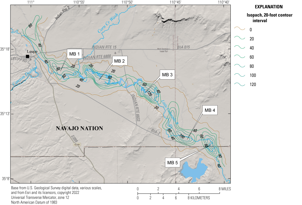
Isopach map showing interpreted thickness of recent alluvium along the Little Colorado River within the study area, near Leupp, Arizona. Thickness of alluvium and proposed microbasins (MB1–5) from Johnson (1999a).
Evolution of the Little Colorado River
Dean and Topping (2019) used historical records of streamflow, suspended sediment discharge, and channel cross-sectional surveys, along with repeat photography, to investigate changes in the geomorphology of the Little Colorado River since the 1920s. One of the parameters they investigated was the total annual flow (TAF). Using streamflow records, they identified the years of 1944 to 1964 and 1996 to 2016 as periods with relatively low TAF, and the years 1926 to 1943 and 1965 to 1995 as periods with relatively high TAF.
They further observed that although TAF has fluctuated in the last 100 years, the magnitude of peak flows during the same time has declined, resulting in a progressive narrowing of the channel since the early 1940s. In addition, large floodplains with dense stands of invasive riparian vegetation have developed as the channel has narrowed. They concluded that “although the initial declines in peak flow were likely caused by changes in climate, subsequent continued declines in peak flow have been most likely caused by a combination of water management actions in the southern parts of the basin and biogeomorphic feedbacks along the length of the Little Colorado River.”
Dean and Topping (2019) cited work by Young and others (2001) showing that for an average year about 36 percent of the annual flow in the Little Colorado River above Winslow was stored in reservoirs or stock ponds, diverted for irrigation, or exported from the basin. They based their analysis on a compilation of surface water supply and cultural depletion estimates from the Arizona Department of Water Resources.
Water Budget
Recharge to the alluvial aquifer in the study area occurs through direct infiltration of precipitation and infiltration of surface-water flow in the Little Colorado River. However, Dohm (1995) concluded that streamflow is the only significant source of recharge to the alluvial aquifer stating that “recharge from precipitation is insignificant because of the small volumes that encounter an extremely high evapotranspiration.” Dohm (1995) further concluded that because winter runoff contributes most of the annual flow for the Little Colorado River, winter runoff is the more important component of flow in regard to aquifer recharge. Estimating recharge to an aquifer from an ephemeral stream is challenging and is further complicated because the recharge rate will likely vary by orders of magnitude over time (Goodrich and others, 2004; Blasch and others, 2004). For these reasons estimating the aquifer discharge may be a better option for gaining insight into long term average recharge rates assuming quasi equilibrium exists between aquifer recharge and discharge.
Withdrawal of water from the alluvial aquifer by pumping is negligible in the study area, leaving evapotranspiration by vegetation the most important form of discharge from the aquifer. Rantz (1968) explained that making rough estimates of average annual evapotranspiration by native phreatophytes in reconnaissance studies is often desirable because “these plants usually draw the great bulk of their water from the underlying ground-water body, either directly or through the capillary fringe.” Doubtlessly, estimating evapotranspiration from invasive phreatophytes is important as well. Dohm (1995) used a consumptive use formula developed by Blaney and Criddle (1962) to estimate the amount of groundwater lost to evapotranspiration from phreatophytes annually from the study area. Using the Blaney and Criddle (1962) formula, he estimated that phreatophytes (mainly tamarisk) within the study area would need about 4.6 ft of groundwater per year. He then estimated the total area of phreatophytic growth for the study area to be 8,030 acres and concluded that the volume density of the phreatophytes was between 20 and 30 percent. Using the following equations, he estimated the volume of groundwater lost to evapotranspiration (VET) in the study area was between 7,390 and 11,080 acre-feet per year (acre-ft/yr).VET = 20% × 4.6 ft/yr × 8,030 acres ≈ 7,390 acre-ft/yrVET = 30% × 4.6 ft/yr × 8,030 acres ≈ 11,080 acre-ft/yr
Johnson (1999a, c) estimated that about 10,440 acre-ft of water leaves the alluvial aquifer in the study area annually by evapotranspiration. Although Johnson provided few details on how this number was derived, it falls within the evapotranspiration range estimated by Dohm (1995). Johnson (1999a, c) also provided an estimate of recharge to the alluvial aquifer based on average bulk porosity and average groundwater-level rise in the aquifer during spring 1998. They estimated the net recharge by infiltration of surface water from the Little Colorado River to be about 9,840 acre-ft for the period March 1998 to March 1999. This recharge number is similar to the annual estimated discharge by evapotranspiration from the aquifer, but actual annual recharge to the alluvial aquifer likely varies widely whereas annual discharge from the aquifer is probably more stable.
Another small component of the water budget for the alluvial aquifer is the inflow of groundwater from alluvium upgradient of the study area and outflow downgradient of the study area. The groundwater gradient in the alluvial aquifer through the study area is very low, likely due in large part to the emplacement of the lava dam downstream. Dohm (1995) used topographic maps to come up with an estimated groundwater gradient of 0.00045. Johnson (1999a, c) used water-level elevations from wells to estimate an average groundwater gradient of 0.001. Based on this gradient, the hydraulic conductivity, and the cross-sectional area of the aquifer at the upstream boundary of the study area, Johnson (1999c) estimated that the alluvial aquifer received about 200 acre-ft of upgradient inflow per year. However, in their preliminary groundwater model, Reclamation (1999) used a lower inflow rate of 109 acre-ft/yr in their steady-state model because they thought the gradient at the upstream end of the study area was lower (0.0004) than the average gradient used by Johnson (1999c). In any case, the estimated inflow from upgradient is small compared to the implied recharge from the Little Colorado River. The calibrated outflow in the Reclamation (1999) steady-state model was just 15.6 acre-ft/yr.
Methods
This study used hydrogeologic information available from previous studies along with ground-based geophysical surveys, water-level and water chemistry data from wells, and simulations of groundwater pumping to develop a better understanding of the hydrogeology of the alluvial aquifer. Also, as part of this study four new observation wells were installed to assess how physical properties varied vertically within the aquifer.
Use of Existing Data
As described in the “Previous Investigations” section, an extensive study was conducted in the late 1990s to characterize the hydrogeology of the alluvial aquifer between Winslow and Leupp. This study was done by the Navajo Nation Department of Water Resources in cooperation with Reclamation and the BIA (Johnson, 1999a–d) for Little Colorado River water-rights negotiations. Hydrogeologic data produced by this effort, including borehole logs, groundwater levels, groundwater chemistry results, aquifer test results, and an isopach map of the alluvial sediment, are used in this report.
Geophysical Surveys
Geophysical techniques used for this study were electrical resistivity tomography (ERT) and gravity. Both of these techniques were used to assess the thickness and extent of alluvial sediment within the study area.
Electrical Resistivity Tomography (ERT)
ERT is a commonly used electrical technique for investigating the subsurface of the Earth. Sedimentary geologic formations like those in the study area tend to have varying resistivity based on their lithology, cementation, and salinity; clay-rich and well-cemented units tend to have low resistivity, and coarser, quartz-rich units like sandstone tend to have higher resistivity. By measuring vertical resistivity cross sections, the location of contacts between formations can be identified. In this study ERT was used to help determine the thickness of the alluvial sediments (that is, the depth of the alluvium–bedrock contact). An Advanced Geosciences Inc. Supersting R8TM multi-channel resistivity/IP meter with a SwitchBox56® was used for the ERT survey. Data were modeled using Advanced Geosciences Inc. Earthimager 2D software. Resistivity measurements were made in dipole-dipole and strong-gradient electrode arrays (Sharma, 1997). For both array types, an electrical current is transmitted into the ground, and the resulting potential differences are measured at the surface. Layers within the Earth that are electrically conductive or resistive will deflect or distort the normal potentials. Dipole-dipole arrays measure apparent resistivity between all possible dipole pairs. Strong gradient arrays measure all adjacent dipoles, which improves weak signals. For each survey line, 56 electrodes (steel rods driven into the ground) at 16.4-ft (5-meter [m]) spacing were extended in leap-frog fashion by moving 28 electrodes between each survey.
Gravity
Measurements of Earth’s gravity field are sensitive to variation in subsurface density. Where the subsurface is less dense than average—for example, an alluvial aquifer—the resultant gravity at the land surface is relatively lower. Where denser material, typically bedrock, is exposed at the surface, gravity is higher. By mapping variations in the gravity field, gravity “lows” (that is, negative gravity anomalies) indicating areas of thicker alluvium can be identified.
Description of Method
Negative anomalies reflect the absence of mass in the alluvial aquifer relative to the surrounding bedrock. Gravity modeling, or inversion, is an iterative process to identify the subsurface density model that accurately reproduces the observed data. Starting with a simple layered model with specified density contrast between layers, the position of interfaces between layers is adjusted so the simulated gravity, also known as the forward model, matches the observations.
Gravity Data
Gravity data (Kennedy, 2023) for this study were collected at 181 stations using ZLS Corporation Burris relative-gravity meters and a Micro-g LaCoste, Inc., A-10 absolute-gravity meter (Kennedy and others, 2021). Drift correction for relative-gravity surveys was carried out using a combination of looping (returning to a base station periodically) and traversing between absolute-gravity stations. Data processing and network adjustment (finding the best-fit solution to all relative- and absolute-gravity data) were carried out using GSadjust software (Kennedy, 2020). Global Positioning System (GPS) data were collected using one GPS receiver as a base station and a second receiver to locate each gravity station. Base station occupations were 4 hours or longer and positioned in the North American Datum of 1983 (2011) epoch 2010.00 reference frame using the National Geodetic Survey Online Positioning User Service. Baseline solutions between the GPS receiver at each gravity station and the base station were processed using Trimble Business Center software. At least 8 minutes of GPS data were collected at each relative-gravity station and at least 20 minutes at each absolute-gravity station. Estimated vertical accuracy is about 2.0 in. (5.08 centimeters [cm]), equivalent to a gravity range of about 0.015 milligal (mGal).
The gravity anomaly was calculated by subtracting the theoretical gravity value for the Geodetic Reference System of 1980 (GRS80) ellipsoid along with standard corrections for elevation (free air) and the Bouguer slab correction (Hinze and others, 2005). Terrain corrections, to account for the gravitational attraction of nearby landforms not related to depth to bedrock, were calculated to a 104-mi distance from each gravity station, assuming 2.67 grams per cubic centimeter (g/cm3) terrain density, from elevation data obtained from The National Map (USGS, 2022a). Between 0 and 1.24 mi (2 kilometers [km]) from each station, corrections were calculated from a 1/3-arc-second (10-m) digital elevation model. Between 1.24 and 104 mi from each station, corrections were calculated from elevation data sampled on a 1,640-ft (500-m) grid. All corrections were calculated using Seequent GM-SYS software (Seequent, 2022). Additional details are in an accompanying data release (Kennedy, 2023).
Gravity interpretation involves several steps to remove influencing factors that are not related to the target of interest (in this study, the thickness of alluvial sediments). First, field data are corrected for time-varying factors, the most important of which is the effect of solid-Earth tides that deform the Earth on daily and twice-daily cycles. Next, the free-air correction is applied to account for the variation in gravity with elevation (weakens as the distance to the Earth’s center of mass increases). The Bouguer correction (Hinze and others, 2005) accounts for the gravitational attraction of the mass between the station elevation and the reference datum elevation (typically zero, or sea level). Finally, terrain corrections account for the topography surrounding the gravity station. After applying these standard corrections, the resultant complete Bouguer anomaly (CBA) reflects both shallow density variations (including low-density basin fill) and deeper, regional variations.
Two additional compilations of CBA data were used in the analysis. Both are regional datasets useful for identifying regional, long-wavelength components of the gravity field but have insufficient resolution to capture the gravitational signature of the alluvial aquifer in the study area. They are used to evaluate and remove the effect of deep, regional geology. First, a compilation of terrestrial data with 3- to 6-mi station spacing in the study area (Sweeney and Hill, 2001), based largely on the National Geodetic Survey compilation (National Geodetic Survey, 1999), provides both the CBA and a second anomaly, the isostatic anomaly, with a regional trend removed. The isostatic anomaly accounts for varying crustal thickness, an important factor for regional-scale interpretation but less so at the local scale of the study area. The GRAV-D dataset provides full-field gravity at flight level, about 15,000 to 17,000 ft above land surface in the study area. Line spacing was about 6.2 mi (10 km) and the along-line distance between points was about 328 to 492 ft (100 to 150 m). The free air anomaly was calculated using provided formulas and MATLAB scripts (GRAV-D Team, 2017) and the CBA calculated using Seequent GM-SYS software. Although the GRAV-D data have insufficient resolution to discern features related to alluvial sediment in the study area, it is a single, consistent dataset as compared to the several datasets collected at different times and with different instruments that comprise the Sweeney and Hill (2001) terrestrial CBA.
Installation of Observation Wells
Four new observation wells were installed as part of this study. These new wells supplemented the nine existing wells that were installed by Johnson (1999a) and used in this study (fig. 5). Johnson (1999a) installed a total of 15 wells (12 observation wells and 3 production wells), but only 9 of the those were found and used in the current study. The well naming convention used by Johnson (1999a) was continued for this study. An example of their naming convention is well BS-20P; the prefix “BS” stands for Birdsprings, “20” is the site number, and “P” stands for production well. In their scheme, a site number with no letter following it is an observation well. The new observation wells were installed at two locations: site 20 established by Johnson (1999a) and a new location numbered site 45 (fig. 5). At each location a deep well and a shallow well were installed. The letter “S” or “D” was added to the site number to indicate if the well was shallow or deep. A list of observation wells used in this study and the type of data collected from each is presented in table 2.
Table 2.
Data types collected from observation wells used in this study, Little Colorado River alluvial aquifer, northeastern Arizona.[USGS, U.S. Geological Survey; ID, identification number.]
| Well name | USGS site ID | Discrete water levels | Continuous water levels | Water-chemistry samples | Well installed by Johnson (1999a) | Well installed as part of this study |
|---|---|---|---|---|---|---|
| BS-06 | 351730110580701 | X | X | X | X | |
| BS-09 | 351630110561601 | X | X | X | X | |
| BS-10 | 351654110564101 | X | X | X | X | |
| BS-17 | 351635110553401 | X | X | X | X | |
| BS-17P | 351634110553401 | X | X | |||
| BS-20 | 351543110531801 | X | X | |||
| BS-20P | 351542110531801 | X | X | X | ||
| BS-20S | 351543110531902 | X | X | X | ||
| BS-20D | 351543110531901 | X | X | X | ||
| BS-22 | 351533110523101 | X | X | |||
| BS-23 | 351441110482001 | X | X | X | ||
| BS-45S | 351610110501002 | X | X | X | ||
| BS-45D | 351610110501001 | X | X | X |
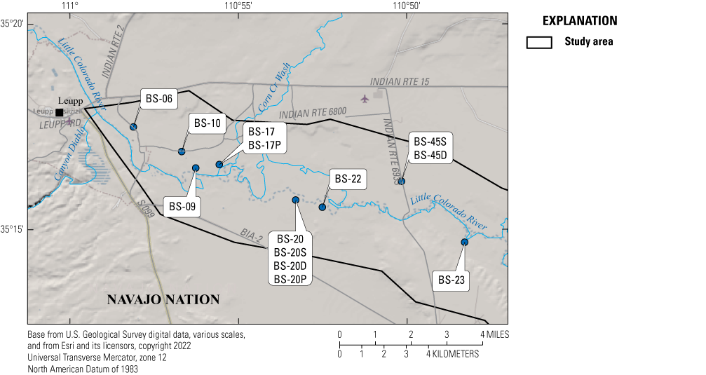
Map showing locations of observation wells used in this study, near Leupp, Arizona. Well locations from the National Water Information System (U.S. Geological Survey, 2022b).
The four new wells were drilled using a hollow-stem auger rig utilizing auger flights with a 4¼-in. inside diameter and a 7⅝-in. outside diameter. The wells were constructed using 2-in. schedule-40 polyvinyl chloride (PVC) threaded casing with a 5-ft length of schedule-40 PVC well screens (0.020 slot). The wells were completed using a medium sand pack from the bottom of the well screen to approximately 2 ft above the screened interval. About 5 ft of time-release coated bentonite tablets were placed above the sand interval with bentonite chips being used to fill the remaining borehole. The surface finish of the wells included a 6-in. diameter steel surface casing with a lockable cap set in a 2-ft square concrete pad (fig 6).
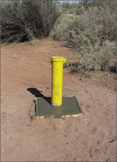
Photograph of surface completion of well BS-45S, near Leupp, Arizona. Photograph by Jon Mason, U.S. Geological Survey, June 10, 2021.
At site 20, well BS-20D was installed to a depth of 136 ft and screened from the bottom of the well up to 131 ft. Based on drill cuttings and material stuck to the auger flights, the lithology of the aquifer penetrated by BS-20D was predominately fine to medium sand with silty clay in places down to a depth of 107 ft. Below 107 ft, the lithology changed to a sticky clay with silt and fine sand. Well BS-20S was installed to a depth of 38 ft and screened from the bottom of the well up to 33 ft. The lithology encountered while drilling BS-20S was the same as that encountered in the upper part of BS-20D. When these wells were installed the water table at site 20 was about 28 ft below the land surface.
The borehole for well BS-45D encountered bedrock at 96 ft. Material on the auger bit indicated the bedrock consisted of light-green sandstone. The well was planned to be installed to a depth of 96 ft with 3 ft of blank casing placed at the bottom of the well to prevent the well screen from contacting weathered bedrock. However, the well unintentionally pulled up 10 ft as the augers were raised so that the final depth for the well was 86 ft with a screened interval of 78 to 83 ft. Based on drill cuttings, the lithology of the aquifer penetrated by the borehole was predominately fine to medium sand. Well BS-45S was installed to a depth of 33 ft and screened from the bottom of the well up to 28 ft. The lithology encountered while drilling BS-45S was the same as that encountered in the upper part of BS-45D. When these wells were installed the water table at site 45 was about 26 ft below the land surface.
Water chemistry samples were collected from all four new observation wells to assess how chemistry varied vertically within the aquifer at each site. In addition, water levels were collected to assess if vertical groundwater gradients were present at the sites. A level survey was conducted between the measuring points of paired wells to ensure their relative water-level elevations were computed accurately. The depth to bedrock value obtained from the borehole for well BS-45D also provided a calibration point to use for gravity data collected near site 45.
Groundwater-Level Measurements
Groundwater levels were monitored at nine observation wells screened in the alluvial aquifer from November 2019 to January 2022. Quarterly water-level measurements using a calibrated electric tape were planned for these wells, but access to the Navajo Nation was limited at times owing to the coronavirus pandemic, so a strict quarterly schedule could not be maintained. Four of the wells also were equipped with recording pressure transducers to provide a continuous record of water-level change. Periodic manual measurements collected at these wells were used to calibrate the transducers and adjust the continuous record. Groundwater levels were monitored in these same observation wells from mid-1997 through early 1999 by Johnson (1999a). A discussion on changes in water levels between the Johnson (1999a) measurements and the measurements collected for this study is provided in the “Results” section.
Groundwater Quality Sampling
Water-chemistry samples were collected from 10 observation wells. Nine of these wells were screened in the alluvial aquifer, whereas one well (BS-20D) was likely screened below the aquifer. Six of the wells sampled had screened intervals ranging from 20 to 60 ft and represent vertically integrated water quality, whereas four wells had screened intervals of 5 ft representing more discrete vertical layers within the aquifer. Water-chemistry samples were collected following standard USGS field protocols (USGS, variously dated). All monitoring wells were constructed with PVC casing and screens and were sampled with a Grundfos Red-Flow 2 submersible impeller stainless-steel monitoring well pump using Teflon tubing. In all but one of the wells, at least three casing volumes of water were pumped prior to sample collection. Well BS-20D (USGS site ID 351543110531901) had a 5-ft screened interval located within a low-permeability silty clay deposit. The well was purged on July 1, 2021, by pumping it nearly dry. The well was purged again on July 6, 2021, prior to sampling. With the exception of well BS-20D, field parameters including pH, water temperature, specific conductance, and dissolved oxygen were monitored while wells were purged to ensure stable parameters were reached prior to sample collection. All water-chemistry samples were analyzed for major ions, nutrients, stable isotopes, and the trace elements arsenic, boron, and iron. Two water-chemistry samples were additionally analyzed for carbon-14 and tritium. Dissolved constituent samples were filtered through a 0.45-micron pore size filter. Unfiltered samples were collected for tritium and stable isotopes. Laboratory analyses for major ions, nutrients, arsenic, boron, and iron were done at the USGS National Water Quality Laboratory (NWQL) according to techniques described in Fishman and Friedman (1989), Fishman (1993), Struzeski and others (1996), and Garbarino and others (2006).
Ratios of the stable isotopes oxygen-18 and oxygen-16 (18O/16O) and deuterium and hydrogen (2H/1H) were measured at the USGS Reston Stable Isotope Laboratory following methods by Révész and Coplen (2008a, b). Uncertainties reported at the 2-sigma level are 0.2 per mil (‰) for oxygen and 2‰ for hydrogen isotopic ratios relative to Vienna Standard Mean Ocean Water. Ratios of these isotopes can be used to estimate the elevation where precipitation fell before becoming recharge to an aquifer. In order to make these estimates, a relationship between elevation and isotopic ratios in precipitation is required. Although developing such a relationship was beyond the scope of the current study, the stable isotope ratios measured in water from the alluvial aquifer can be used in future studies.
Tritium (3H) is a useful tracer for determining if there is a component of water recharged during or after the period of thermonuclear bomb testing in the 1950s and 1960s. Tritium occurs naturally in the atmosphere in extremely small concentrations, but the detonation of above ground thermonuclear devices increased the tritium concentration in the atmosphere by many orders of magnitude over natural levels. Tritium in the form of water can then fall as precipitation from the atmosphere and become recharge for aquifers. Atmospheric testing of thermonuclear devices began in 1952 and largely ended in 1963 with the signing of the Nuclear Test-Ban Treaty by most nations possessing nuclear weapons. Tritium was assessed with a categorical age classification as proposed by Beisner and others (2017): less than 1.3 picocuries per liter (pCi/L) is considered pre-modern (before 1952), greater than 12.8 pCi/L is modern (primarily after 1952), and values between the thresholds indicate a possible mixture of pre-modern and modern water. Tritium samples were analyzed by the University of Miami Tritium Laboratory in Miami, Florida, using the electrolytic enrichment and gas-counting method (Thatcher and others, 1977), with a reporting limit of 0.3 pCi/L.
Carbon-14 and 13/12C were analyzed by the National Ocean Sciences Accelerator Mass Spectrometry (NOSAMS) facility at Woods Hole Oceanographic Institution. Carbon-14 can be used to estimate the age of groundwater recharge, but the geochemical modeling required was beyond the scope of the current study.
Quality assurance for this study was maintained through the use of standard USGS training of field personnel, use of standard USGS field protocols (USGS, variously dated), collection of quality control (QC) samples, and thorough review of the analytical results. All USGS scientists involved with this study have participated in the USGS National Field Quality Assurance Program, which is an annual assessment of skills in analyzing water-chemistry samples for pH, electrical conductivity, and alkalinity.
An equipment blank was collected prior to collection of the first environmental sample to ensure the equipment decontamination procedures used between sample collections were adequate. Concentrations of analytes in the equipment blank were below the NWQL method detection limits (table 3).
Table 3.
Chemical analyses of equipment blank water sample, Little Colorado River alluvial aquifer, northeastern, Arizona.[USGS, U.S. Geological Survey; ID, identification number; mg/L, milligrams per liter; µg/L, micrograms per liter; <, less than.]
Sequential replicate QC samples were collected at monitoring wells BS-20P and BS-45S to better understand potential variability associated with field conditions and field and laboratory procedures (table 4). For all constituents, relative percentage differences (difference in sample results divided by the mean result) measured between results from the environmental sample and replicate sample from Well BS-20P ranged from 0 to 3.5 percent. Relative percentage differences were slightly more between results from well BS-45S ranging from 0 to 7.3 percent. However, only three constituents (arsenic, fluoride, and iron) had differences greater than 5 percent. These two replicate samples suggests that there is an acceptably low level of variability affecting the data; no QC data were collected to assess potential bias affecting the data.
Table 4.
Comparison of chemical analyses of replicate and environmental water-chemistry samples from monitoring wells BS-20P and BS-45S, Little Colorado River alluvial aquifer, northeastern Arizona.[USGS, U.S. Geological Survey; ID, identification number; °C, degrees Celsius; µS/cm, microsiemens per centimeter at 25 °C; mg/L, milligrams per liter; µg/L, micrograms per liter; <, less than; --- no data.]
Well-Field Pumping Scenarios
Hypothetical single well and multiple well pumping scenarios were conducted to investigate the feasibility of using groundwater from the alluvial aquifer for crop irrigation in the study area. The aquifer tests conducted by Johnson (1999a) indicated that transmissivities in the alluvial aquifer were generally low making the success of high-volume irrigation wells doubtful. The pumping scenarios were done using the Forward Solution Wizard in AQTESOLV version 4.5 aquifer test analysis software (Duffield, 2007). The AQTESOLV Forward Solution Wizard was designed to predict hydraulic response in an aquifer for a specified set of hydraulic properties, pumping rates, well locations and boundary conditions. The Neuman (1974) method was used for the pumping scenario forward solutions. This method was chosen because it is one of the methods used by Johnson (1999a) to analyze aquifer test results and is the method he used to estimate the specific yield of the alluvial aquifer.
Johnson (1999a) conducted three multiwell aquifer tests and eight single-well aquifer tests. Because multiwell aquifer tests generally characterize a larger portion of the aquifer than do single well aquifer tests, the hydraulic property values estimated from multiwell aquifer tests were considered for use in the forward solutions. Of the multiwell aquifer tests, only the values for transmissivity, specific yield, and storativity from the aquifer test conducted closest to the proposed agricultural fields (site 17) were used in the forward solutions (table 5). Using average values from all three aquifer tests was considered, but Johnson (1999a) deemed the results from site 20 non-characteristic of the alluvial aquifer because the observation well at site 20 was screened below the alluvial aquifer. Further, aquifer test results from site 22 were similar to the results from site 17, so using an average of the two tests was deemed unnecessary.
Table 5.
Estimated hydraulic properties used in forward well-field pumping scenarios.[ft2/d, feet squared per day; ft/d, feet per day.]
| Hydraulic property | Hydraulic property value | Source of value |
|---|---|---|
| Transmissivity (T) | 4,300 ft2/d | Johnson (1999a) |
| Storativity (S) | 1.86 × 10⁻⁵ | Johnson (1999a) |
| Specific yield (Sy) | 0.19 | Johnson (1999a) |
| Hydraulic conductivity | 70 ft/d | Johnson (1999a) |
| Vertical-to-horizontal hydraulic conductivity anisotropy ratio (β)1 | 0.001 | This study |
| Vertical-to-horizontal hydraulic conductivity anisotropy ratio (Kz/Kr)2 | 3.027 × 10⁻⁴ | This study |
Johnson (1999a) does not provide a value for the anisotropy ratio between vertical hydraulic conductivity and horizontal hydraulic conductivity. This ratio was estimated using the transmissivity, storativity, and specific yield values provided by Johnson (1999a) for the site 17 aquifer test. The fit between the drawdown data and curves from the Neuman (1974) method indicates a small anisotropy ratio (3.027×10⁻⁴). A small anisotropy ratio, where vertical hydraulic conductivity is much less than horizontal hydraulic conductivity, is expected for the alluvial aquifer given there are numerous silt and clay layers reported by Johnson (1999a) in the lithologic descriptions from well bores.
The simulations of well pumping are not intended to provide specific well-field designs for implementation but are intended to explore the feasibility of using groundwater from the alluvial aquifer for irrigation in the study area and to assess if such water use can be sustainable on a scale beneficial to the local population. The pumping scenarios tested used a withdrawal amount of 400 acre-ft per irrigation season. This number was arrived at by assuming that 100 acres of crops would be irrigated using 4 acre-ft of water per acre. For comparison, Frisvold (2015) reported the average annual water use across all crops in Arizona was about 4.2 acre-feet per acre (acre-ft/acre) in 2013. Crops like alfalfa used more water (>5 acre-ft/acre), whereas crops like corn and vegetables used less water (~3 acre-ft/acre). The irrigation season was assumed to be 92 days long running from June through August. Assuming continuous pumping for 92 days, a pumping rate of about 1,000 gallons per minute (gal/min) is required to produce 400 acre-ft of irrigation water.
Results
Geophysical Surveys
ERT and gravity geophysical techniques were used to assess the thickness and extent of alluvial sediment within the study area. Geophysical data collected for this study are available from Macy and Mason (2023) and Kennedy (2023). One goal of this study was to explore whether a continuous paleocanyon or paleovalley incised into bedrock and filled with Little Colorado River alluvial sediments extends through the study area as opposed to the series of microbasins proposed by Johnson (1999a). The geophysical surveys conducted as part of this study show that a deeper bedrock channel likely exists between MB2 and MB3 (fig. 4) that is located to the north of the saddle depicted in the Johnson (1999a) isopach map of the study area. The surveys further show that a small bedrock channel may extend out of the study area to the northwest of MB1. However, the results collected between MB3 and MB4 do not indicate the presence of a bedrock channel. Data are insufficient between the other microbasins to fully test which hypotheses is correct.
ERT data collected along 4 transects are discussed relative to 2 areas: the area between MB2 and MB3 along the Transwestern Road, and MB4 near the intersection of BIA roads 2 and 71. ERT transect 2.5 is so named because it is located between MB2 and MB3 (fig. 7A). All 4 transects contain the same 2 stratigraphic layers: an upper layer of Quaternary alluvium, which represents the alluvial aquifer where the layer is saturated, and a lower bedrock layer consisting of Triassic bedrock. The geologic maps of the area by Ulrich and others (1984) and Billingsley and others (2013) indicate bedrock under the ERT transects could either be the Moenkopi Formation or the Chinle Formation. The depth to the geologic contact between the Moenkopi and Chinle Formations is not known in the area of the transects, and the Moenkopi and Chinle Formations likely have similar electrical properties so that the contact may not be obvious based on the ERT results alone. Because both formations contain abundant fine-grained sediments, they are likely hydrologically similar and do not readily allow for the transmission of groundwater. For these reasons the Moenkopi and Chinle Formations were grouped as “Triassic bedrock.”
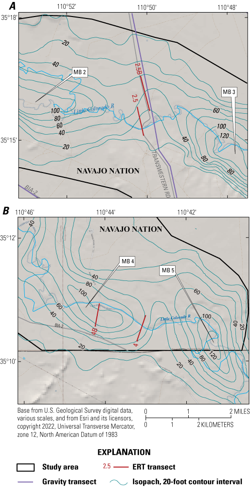
Map of electrical resistivity tomography (ERT) transects 2.5 and 2.5B (A) and transects 4 and 4B (B) with isopachs showing interpreted thickness of recent alluvium along the Little Colorado River, near Leupp, Arizona. Thickness of alluvium and proposed microbasins (MB2–5) from Johnson (1999a). Gravity transects within the extent of the maps also are shown as a reference.
In general, areas with resistivity values greater than about 100 ohm-meters (ohm-m) along ERT transects 2.5 and 2.5B (fig. 8) are interpreted to be Quaternary alluvium. Resistivity values less than 100 ohm-m are interpreted as Triassic bedrock. In ERT transect 2.5, the bedrock is very near the surface from stations −197 to 689 (fig. 8A). Beginning around station 689, Quaternary alluvium begins to thicken as the transect proceeds to the northwest and reaches a thickness of around 100 ft. ERT transect 2.5B is a continuation of transect 2.5, although it begins about ¼ mi to the east of where transect 2.5 ends to accommodate crossing the Little Colorado River channel (fig. 7A). It shows that the Quaternary alluvium continues to thicken to around 120 ft by the middle of the transect and remains that thick to the end. The depth to groundwater is about 30 ft below land surface in this area indicating that the alluvial aquifer varies in thickness from 0 ft in the southeastern half of ERT transect 2.5 to around 90 ft in the northwestern half of transect 2.5B.
Areas of ERT transects 4 and 4B (fig. 9) with resistivity values greater than about 100 ohm-m also are interpreted to be Quaternary alluvium, with values lower than 100 ohm-m being interpreted as Triassic bedrock. ERT transect 4 crosses the current channel of the Little Colorado River at a perpendicular angle, whereas ERT transect 4B, about 1 mi downstream, approaches the Little Colorado River at a perpendicular angle but remains on the south side of the current channel (fig. 7B).
The modeling results of ERT transect 4 are less consistent and more challenging to interpret than the other transects, which is indicated by the dashed line on the left half of the transect denoting the contact between Quaternary alluvium and Triassic bedrock (fig 9A). Based on the modeling results, the southwestern half (left side) of the transect appears to have a depth to bedrock of around 100 ft, whereas the northeastern half (right side) has a depth to bedrock of around 60 ft. Groundwater levels in this area also are around 30 ft below land surface making the aquifer thickness along the transect between about 30 and 70 ft. The data and modeling are more consistent for ERT transect 4B. They indicate a depth to bedrock between about 90 and 120 ft, with a corresponding aquifer thickness ranging from about 60 to 90 ft (fig 9B).
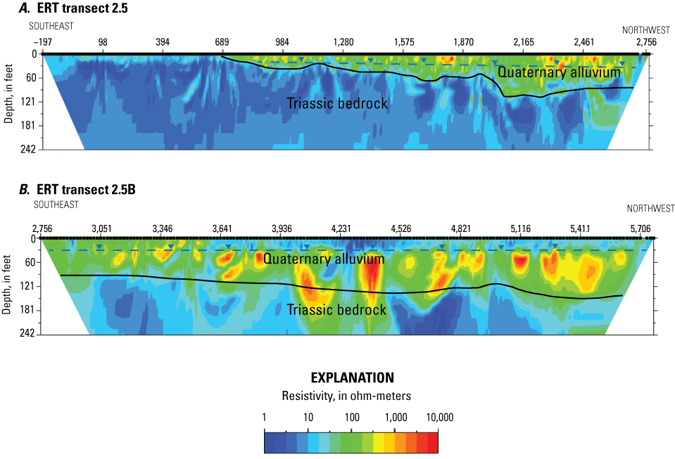
Inverse model resistivity sections of electrical resistivity tomography (ERT) transects 2.5 (A) and 2.5B (B), east of Leupp, Arizona. Areas with warm colors (yellow, orange, red) have higher resistivity, and areas with cool colors (purple, blue, green) have lower resistivity. Areas of high resistivity are interpreted to be Quaternary alluvium, whereas areas of low resistivity are interpreted to be Triassic bedrock. Dashed blue line in alluvium shows approximate depth to water table of 30 feet in the alluvial aquifer. Locations of ERT transects shown in figure 7.
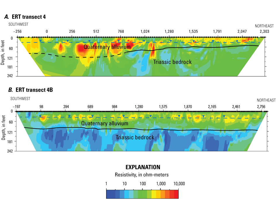
Inverse model resistivity sections of electrical resistivity tomography (ERT) transects 4 (A) and 4B (B), east of Leupp, Arizona. Areas with warm colors (yellow, orange, red) have higher resistivity, and areas with cool colors (purple, blue, green) have lower resistivity. Areas of high resistivity are interpreted to be Quaternary alluvium, whereas areas of low resistivity are interpreted to be Triassic bedrock. Dashed blue line in alluvium shows approximate depth to water table of 30 feet in the alluvial aquifer. Locations of ERT transects shown in figure 7.
Gravity Interpretation
Gravity interpretation begins with the CBA, which represents density disturbances relative to a homogeneous Earth. The two independent sources of regional CBA—terrestrial data compiled by Sweeney and Hill (2001), and airborne data collected by National Geodetic Survey (GRAV-D Team, 2018)—show some similarities but also marked differences (fig. 10). The study area is centered on a gravity high in both datasets, near Leupp, that slopes towards more negative gravity values to the southeast. The magnitude of gravity change across the study area is about 8 to 14 mGal for the GRAV-D and terrestrial datasets, respectively, more than would be expected from variation in alluvium thickness of 0 to 100 ft. Other prominent features that appear in both datasets are a gravity low around the Flagstaff area and a gravity high about 50 mi northwest of the study area. These most likely relate to structures in the Proterozoic Unkar and Chuar Groups at depths more than 3,000 ft below land surface (Seeley and Keller, 2003) and, to a lesser degree, igneous formations related to the San Francisco Volcanic Field (Mickus and Durrani, 1996).
Because of large spacing between observations, neither regional CBA dataset captures the gravity lows associated with Little Colorado River alluvial sediment. In the study area none of the terrestrial data stations used to create the CBA are near the Little Colorado River channel (fig. 10A). Therefore, these data are useful for removing the effect of regional gravity variation unrelated to alluvial sediment. The GRAV-D CBA (fig. 10B) could be used for the same purpose, but it has higher levels of high-frequency noise (GRAV-D Team, 2017) and attempts to transfer the airborne data from the observation height to the land surface (that is, downward continuation) were unsuccessful.
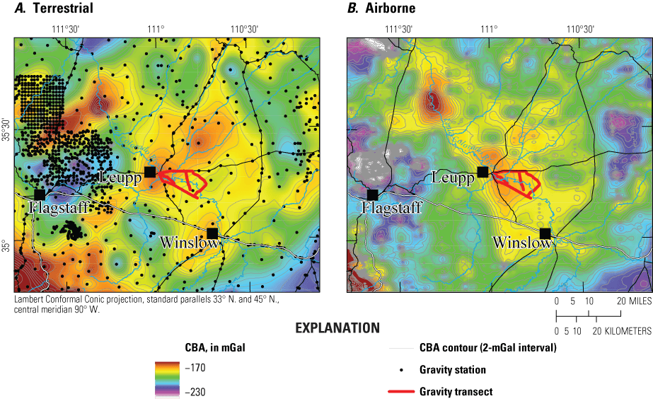
Maps of complete Bouguer gravity anomalies (CBAs) calculated from terrestrial data (A) (Sweeney and Hill, 2001) and airborne data (B) (GRAV-D Team, 2018), northeastern Arizona.
For data newly collected for this study, the local residual was calculated by subtracting the terrestrial regional CBA (fig. 10A) from the observed CBA (fig. 11A). This accounts for the lower-to-the-southeast trend within the study area observed in both regional datasets (fig. 10) that is likely unrelated to the thickness of alluvial sediment. After subtracting, the resultant local residual (fig. 11B) shows gravity variations related to the depth of alluvium. Higher gravity values (darker blue colors) are on areas of bedrock outcrop and thin alluvial cover, including along most of the roads that bound the study area. Obvious gravity lows (white circles, fig. 11B) on gravity transects 1 and 3 likely correspond to the thickest alluvium along these gravity transects.
At the northwest corner of the study area, alluvium appears to be thin and bounded by the Moenkopi Formation outcropping to the west and the Chinle Formation just to the north (Billingsley and others, 2013). A subtle gravity low at the west end of gravity transect 2 marks the location of the thickest part of the alluvium and where a bedrock channel may have exited the study area, about 600 ft east of the present-day Little Colorado River channel. At the southeast end of gravity transect 1, and the western part of gravity transect 5, alluvium appears to reach its deepest and broadest extent, with the alluvial channel extending the entire width of the present-day channel and into the floodplain south of gravity transect 5. However, the extent of deep alluvium along gravity transect 5 (fig. 11B, light-colored circles) is limited and much smaller than the extent of surface alluvium. At gravity transect 3, alluvium likely does not extend southward past the present-day channel, and the thickest alluvium is towards the north end of the transect, nearly 2 mi north of the present-day channel. The Chinle Formation is mapped at the south end of gravity transect 3 (Billingsley and others, 2013) and likely extends to, or nearly to, the present-day channel. Along gravity transect 4, and in particular the southwest-northeast trending segment that crosses the Little Colorado River channel, alluvium appears to be relatively thin and coincides with the present-day channel.
Gravity data were quantitatively interpreted by modeling two-dimensional (2D) cross sections. Insufficient data were available in the channel longitudinal direction to interpolate a 2D plan-view gravity anomaly required for three-dimensional (3D) inversion and owing to this lack of data, the multiple sub-basin hypothesis of Dohm (1995) and Johnson (1999a) could not be evaluated. However, the gravity method appears to work well for identifying alluvial thickness in the study area and the analysis could be expanded with additional data.
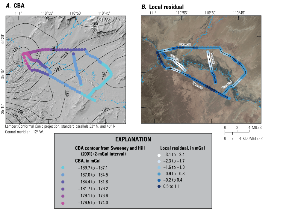
Maps of gravity data reduced to the complete Bouguer gravity anomaly (CBA) (A) and the local residual (the CBA with the regional trend subtracted) (B) along gravity transects, near Leupp, Arizona.
The local gravity anomaly is simulated as 2D prisms with infinite extent perpendicular to the cross section. Different densities were evaluated for unsaturated sediment (1.2–1.9 g/cm3), saturated sediment (1.5–2.0 g/cm3), and bedrock (Moenkopi and Chinle Formations, 2.5–2.67 g/cm3). The strike of the sloping contact between the Chinle Formation and the underlying Moenkopi Formation, a primary stratigraphic feature in the study area, is parallel or subparallel to gravity transects 1 and 3 and was not simulated. For the southern part of gravity transect 4, a density contrast between these formations parallel to the northeast-dipping contact was simulated in the density inversion. After constructing a reasonable starting cross section for each profile, the elevation of the saturated alluvium/bedrock contact was adjusted using a Marquardt inversion algorithm as implemented in GM-SYS software (Seequent, 2022).
For gravity transects 1 and 3, where there are borehole logs for comparison, a large density contrast was required to match the observed depth to bedrock. For gravity transect 1, values of 1.2 g/cm3, 1.8 g/cm3, and 2.67 g/cm3 were used for the densities of unsaturated alluvium, saturated alluvium, and bedrock, respectively, to match the observed depth to bedrock from the borehole log at well BS-06: 60 ft (fig. 12A). Using these same densities for gravity transect 3, bedrock at BS-45D, estimated at 95 ft below land surface from borehole logs, was estimated at 170 ft below land surface (fig. 12B). The alluvium/bedrock contact can be adjusted upward to match the observed depth to bedrock, but this requires unrealistically low densities for unsaturated and saturated alluvium such as 1.1 g/cm3 and 1.27 g/cm3, respectively (other combinations would also replicate the observed gravity values).
For the southwest-northeast trending part of gravity transect 4 that crosses the Little Colorado River, gravity data indicate a relatively thin aquifer (fig. 12C). Unlike gravity transects 1 and 3, gravity transect 4 has a decreasing trend to the northeast. In part, this may be caused by the sloping, down-to-the-northeast contact between lower density shale in the Chinle Formation and the higher density Moenkopi Formation. Including this feature in the model cross section imparts a decreasing trend to the simulated gravity value, but reasonable density values (2.67 g/cm3 and 2.55 g/cm3 for Moenkopi and Chinle Formation density, respectively) were unable to simulate the slope of the gravity anomaly at the left (southwest) end of the transect and caused too-low gravity values at the northeast end. The discrepancy between simulated and measured gravity values at the northeast end of the transect may be caused by an incorrect correction induced by subtracting the regional CBA, or by density features not present in the model, such as density variation in the deeper Paleozoic or Proterozoic rocks. Regardless, the data suggest the alluvial aquifer is less extensive along this transect than previously mapped (Billingsley and others, 2013).
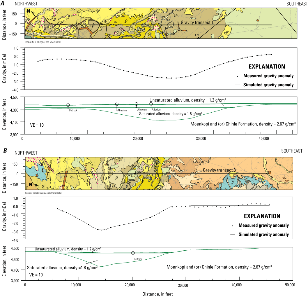
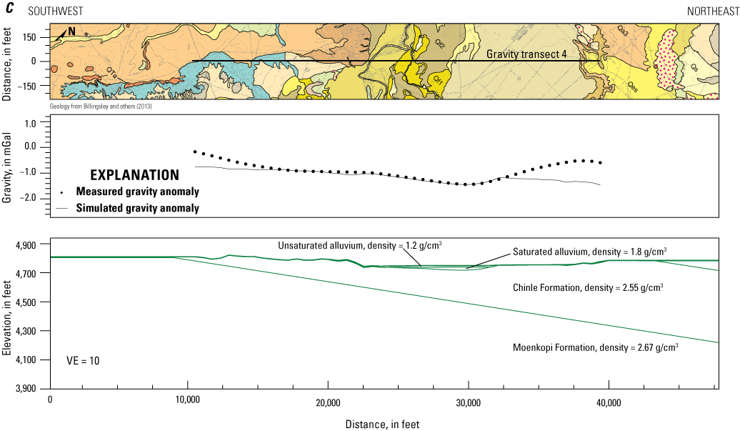
Cross-sectional plots of density along gravity transect 1 (A), transect 3 (B), and transect 4 (C), near Leupp, Arizona. Top, Geology (plan view) from Billingsley and others (2013). Middle, Measured local gravity anomaly (black dots) and simulated local gravity anomaly (black line). Bottom, Interpreted density profile. Hollow circles are boreholes labeled with the material at total depth. All map units are Quaternary surficial deposits, with the exception of the Triassic Chinle Formation in light blue (B, C). The locations of the gravity transects is shown in figure 11B. mGal, milligal; g/cm3, grams per cubic centimeter; VE, vertical exaggeration.
Together, the gravity data indicate a relatively thick, broad alluvial aquifer in the vicinity of gravity transects 1 and 3, and a much thinner aquifer in the vicinity of gravity transect 4. Reasonable density contrasts produced depths-to-bedrock greater than were observed in borehole logs (that is, the gravity lows are relatively large compared to the relatively shallow bedrock observed in boreholes). One contributing factor may be weathering of the bedrock prior to burial, thereby lowering its density (Wald and others, 2013).
Groundwater-Level Measurements
Hydrographs of groundwater levels collected by this study from the 5 intermittently measured wells and the 4 continuously recording wells are shown in figure 13A. For comparison, hydrographs showing the water levels collected from the same wells by Johnson (1999a) are shown in figure 13B. All the hydrographs in figure 13B have a characteristic pattern, which shows rising water levels in early to mid-spring 1998, followed by declining water levels from late spring through the summer months. This pattern corresponds well to the conceptual water budget described by Johnson (1999a), which assumes most recharge to the aquifer occurs as infiltration from the Little Colorado River during the spring runoff season and the main discharge from the aquifer is in the form of evapotranspiration from riparian vegetation. The four hydrographs from wells with continuous water-level records in figure 13A show a similar but more subdued pattern of water-level fluctuations in 2020 with an even more attenuated response in 2021.
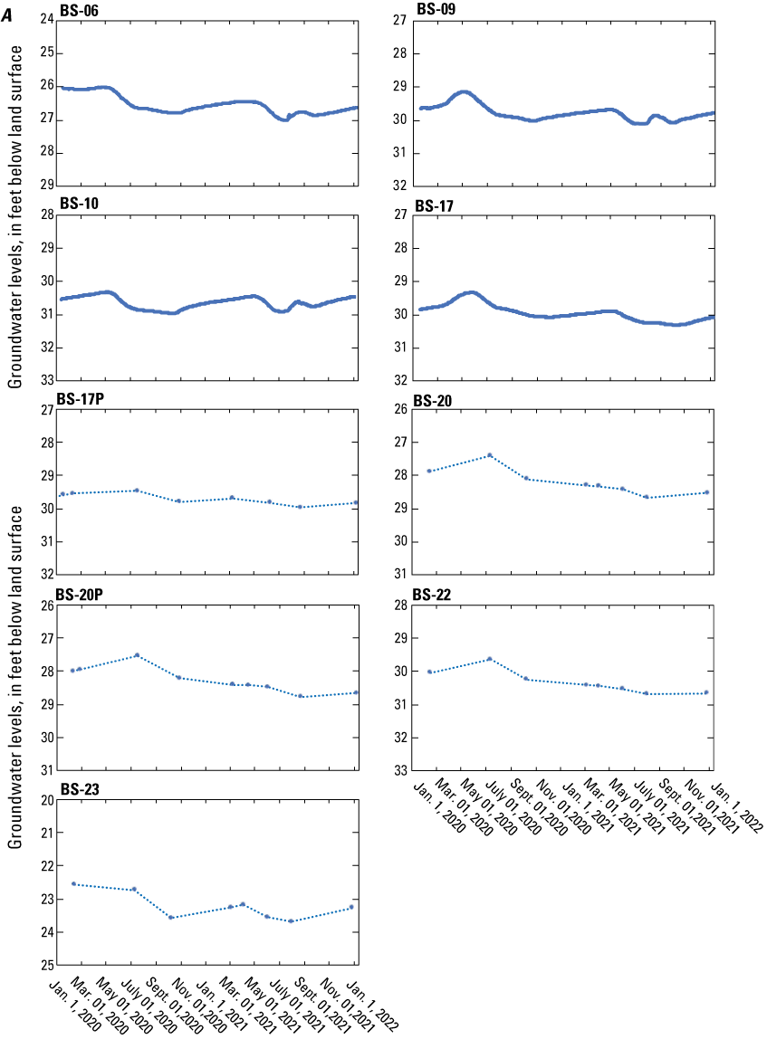
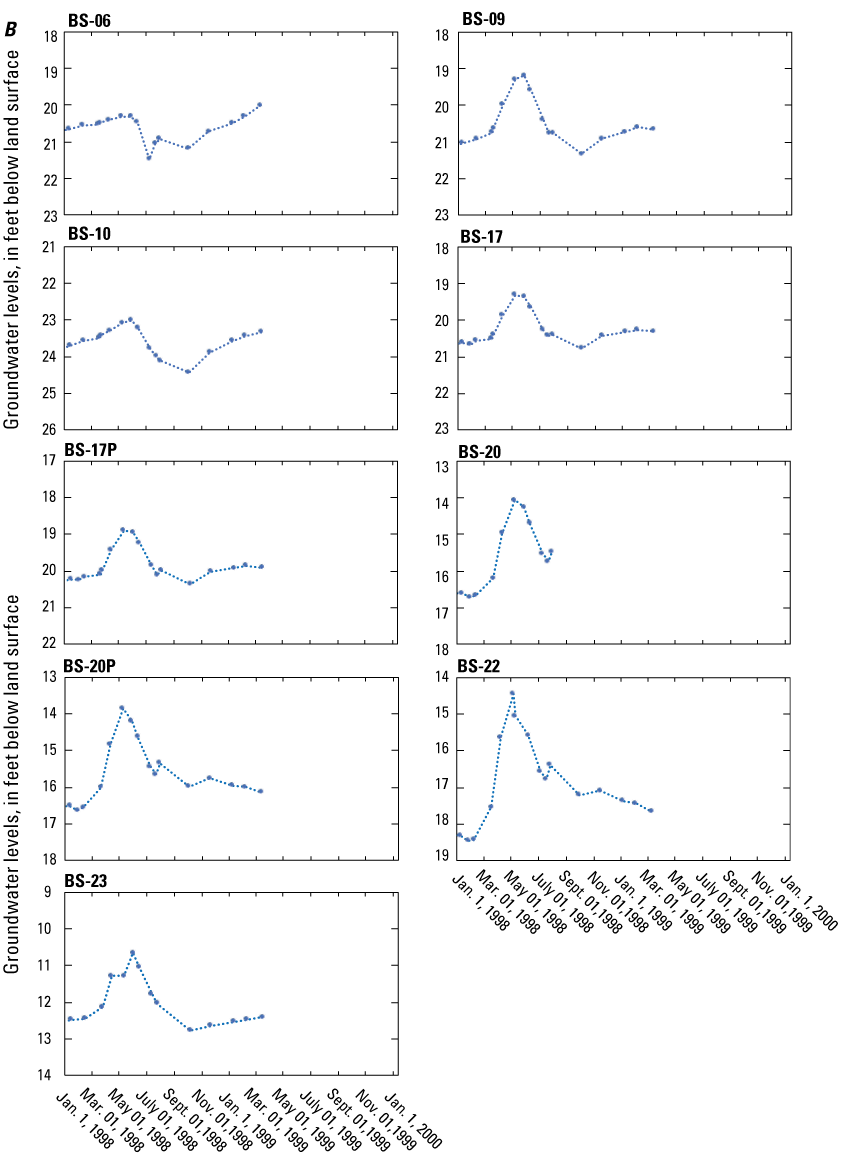
Hydrographs of groundwater levels from 5 wells measured intermittently and from 4 continuously recording wells (locations of wells shown in fig. 5). A, Groundwater levels collected for this study, January 2020 through December 2021. B, Groundwater levels collected by Johnson (1999a), January 1998 through March 1999. x-axes of A and B display the same months (of different years) to aid comparison of water levels between the two time intervals.
Hydrographs of mean daily discharge are shown from streamgage 09402000, Little Colorado River near Cameron, Ariz., for January 2020 through December 2021 (fig. 14A) and January 1998 through December 1999 (fig. 14B). Although this streamgage is about 60 mi downstream of the study area, it can still provide an index of change in snowmelt runoff through the study area between years because most snowmelt in the river comes from the Mogollon Rim upstream of the study area. There was about 26 percent less annual discharge measured at the Cameron streamgage in the late-winter through spring months of 2020 (January 1 through June 19, 2020) than there was in 1998 (January 1 through June 19, 1998). Further, there were about 44 percent fewer days with mean daily flow above 500 cubic feet per second (ft3/s) at the streamgage during these months in 2020. The lower late-winter through spring runoff in 2020 likely played a role in the more subdued response of groundwater levels in study area wells when compared to 1998 water levels during the same months. Figure 14A shows there was essentially no late-winter through spring runoff at the Cameron streamgage in 2021. However, a small amount of water-level recovery is visible in study area wells during spring 2021. This recovery is likely due to the cessation of evapotranspiration by floodplain vegetation and underflow of groundwater into the alluvial aquifer.
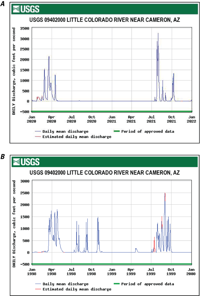
Plots of daily mean discharge for streamgage 09402000, Little Colorado River near Cameron, Arizona, from January 2020 to December 2021 (A) and from January 1998 to December 1999 (B).
Comparison between the two sets of hydrographs (fig. 13) show that water levels have declined in all of the wells from the earlier period (1998–99) to the more recent period (2020–21). Comparison of water-level changes between the two time periods is not straightforward owing to the seasonal variability in water levels. To simplify the comparison, the lowest water levels recorded at each well during both time periods were compared. Using this method, the decline in water levels ranged from 5.6 ft at BS-06 to 12.2 ft at BS-22.
Water levels were measured in sets of paired wells at sites 20 and 45 to evaluate vertical groundwater gradients. At site 45 a shallow well was screened near the water table of the alluvial aquifer, whereas a deeper well was screened near the bottom of the alluvial aquifer. At site 20 a shallow well was again screened near the water table of the alluvial aquifer, but the deeper well was screened below the alluvial aquifer in a clay-rich sedimentary layer that acted as an aquitard.
Table 6 shows the water-level measurements collected at the two sets of paired wells. A level survey was conducted between the measuring points of paired wells to ensure their relative water-level elevations were computed accurately. The vertical gradient at site 45 ranged from +0.01 to −0.18 ft. The difference in water levels (deep minus shallow such that a positive difference indicates an upward gradient and a negative difference indicates a downward gradient) from the paired wells at site 20 were more variable, ranging from −2.87 to +0.68 ft. The difference in elevation between the first set of measurements (−2.87 ft) collected on July 1, 2021, may reflect that well BS-20D still had not fully recovered from being bailed after installation 3 weeks earlier. Given the thick clay-rich layer that well BS-20D was completed in, and the amount of time it took for the well to recover after bailing, it is probable that the barometric efficiency of the well was very low and that the differences in water-level elevation measured between the deep and shallow wells had more to do with how each well responded to changes in ambient air pressure than with vertical groundwater gradients.
Table 6.
Comparison of water levels measured in paired shallow and deep wells, Little Colorado River alluvial aquifer, northeastern Arizona.[Water-level data available from U.S. Geological Survey (2022b). MP, measuring point; ft, feet; elev., elevation; diff., difference.]
Groundwater Geochemistry
Groundwater geochemistry is described in this section for general chemical properties and groundwater age. The geochemistry results are located in appendix 1 and also are available from the USGS National Water Information System (NWIS) database (USGS, 2022b). Groundwater samples were collected from 9 wells completed in the alluvial aquifer and from 1 well installed below the alluvial aquifer. The sampled wells ranged in depth from 33 to 136 ft. The implications of aquifer geochemistry on possible sources of groundwater recharge and on the suitability of the water for use in crop irrigation is examined later in the “Discussion” section.
General Chemistry
There was wide variability in the concentrations of total dissolved solids from samples which ranged from 915 to 6,330 milligrams per liter (mg/L) (appendix 1). Samples from the nine wells completed within the aquifer had a sodium-chloride water type, which is unusual for an alluvial aquifer (fig. 15). Sodium chloride, known as the mineral halite in the solid phase, is very soluble in water and tends to pass through open flow systems rather than becoming concentrated. The sample from the one well completed below the aquifer (BS-20D) had a mixed water type. Sodium was the dominant cation present in the sample, but chloride made up less than 50 percent of the total anion content of the sample (appendix 1).
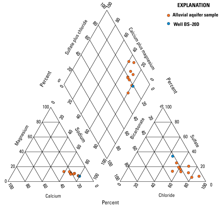
Piper diagram (Piper, 1944) showing relative ionic compositions of 9 groundwater-chemistry samples collected from the Little Colorado River alluvial aquifer and 1 sample from well BS-20D screened below the aquifer, northeastern Arizona.
Concentrations of all the analyzed constituents in samples from wells were less than current U.S. Environmental Protection Agency (EPA) maximum contaminant levels (MCLs) (EPA, 2023a). However, concentrations of both chloride and total dissolved solids exceeded the secondary maximum contaminant levels (SMCLs) (EPA, 2023b) in samples from all wells. The SMCLs for chloride and total dissolved solids are 250 mg/L and 500 mg/L, respectively. In addition, the SMCL for iron (300 micrograms per liter [µg/L]) was exceeded in samples from BS-06 and BS-10, whereas the SMCLs for iron and sulfate (250 mg/L) were exceeded in the sample from BS-23 (figs. 16, 17). SMCLs are non-mandatory water quality standards established by the EPA as guidelines to assist public water systems in managing their drinking water for aesthetic considerations such as taste, color, and odor. These contaminants are not considered to present a risk to human health at the SMCL, but given that many of the samples contained total dissolved-solids concentrations exceeding the SMCL by several times, treatment would likely be required in most areas before the water would be suitable for domestic uses.
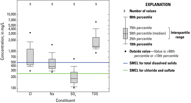
Boxplots of chloride, sodium, sulfate, and total dissolved-solids concentrations from nine water-chemistry samples collected from the Little Colorado River alluvial aquifer, northeastern Arizona, for this study. mg/L, milligrams per liter; SMCL, secondary maximum contaminant level (U.S. Environmental Protection Agency, 2023b).
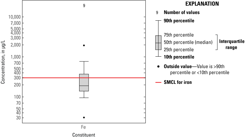
Boxplot of iron concentrations from nine water-chemistry samples collected from the Little Colorado River alluvial aquifer, northeastern Arizona, for this study. μg/L, micrograms per liter; SMCL, secondary maximum contaminant level (U.S. Environmental Protection Agency, 2023b).
A comparison between major ion water chemistry from samples collected as part of the current study and chemistry from samples collected by Johnson (1999b) is presented in table 7. Most major ion concentrations increased between the collection of the 1998 samples and the collection of samples for this study, although there were a few exceptions. Most notably, the total dissolved-solids concentration and many of the constituent ion concentrations, in samples from well BS-09 decreased (table 7). The largest changes in total dissolved solids occurred at wells BS-06 and BS-10, where the concentrations went from 2,570 and 1,510 mg/L, respectively, in the 1998 samples to 3,690 and 2,120 mg/L, respectively, in the 2019 samples, an increase of more than 40 percent at both wells (table 7).
Table 7.
Comparison of chemical analyses from Johnson (1999b) and this study of water-chemistry samples from six monitoring wells, Little Colorado River alluvial aquifer, northeastern Arizona.[USGS, U.S. Geological Survey; ID, identification number; mg/L, milligrams per liter; °C, degrees Celsius; ND, not detected at minimum detection level; ---, no data.]
| Study | Date of samples | Dissolved constituents | |||||||
|---|---|---|---|---|---|---|---|---|---|
| Calcium (mg/L as Ca) |
Magnesium (mg/L as Mg) |
Potassium (mg/L as K) |
Sodium (mg/L as Na) |
Bicarbonate (mg/L) |
Chloride (mg/L as Cl) |
Sulfate (mg/L as SO4) |
Solids, residue at 180 °C (mg/L) | ||
| Johnson (1999b) | 7/21/1998 | 196 | 48.4 | ND | 587 | 378 | 951 | 517 | 2,570 |
| This study | 12/17/2019 | 341 | 90.5 | 6.48 | 822 | 375 | 1,570 | 629 | 3,690 |
| Percent change | --- | 74.0 | 87.0 | --- | 40.0 | −0.8 | 65.1 | 21.7 | 43.6 |
| Johnson (1999b) | 7/21/1998 | 118 | 34.9 | 1.56 | 346 | 300 | 604 | 201 | 1,530 |
| This study | 12/19/2019 | 59.6 | 17.9 | 2.69 | 390 | 305 | 506 | 141 | 1,290 |
| Percent change | --- | −49.5 | −48.7 | 72.4 | 12.7 | 1.7 | −16.2 | −29.9 | −15.7 |
| Johnson (1999b) | 7/21/1998 | 80.5 | 23.6 | 1.03 | 444 | 300 | 639 | 232 | 1,510 |
| This study | 12/19/2019 | 148 | 45.7 | 3.94 | 548 | 317 | 948 | 206 | 2,120 |
| Percent change | --- | 83.9 | 93.6 | 282.5 | 23.4 | 5.7 | 48.4 | −11.2 | 40.4 |
| Johnson (1999b) | 7/18/1998 | 34.6 | 9.76 | 1.08 | 271 | 284 | 271 | 146 | 896 |
| This study | 12/17/2019 | 40.9 | 12.1 | 2.05 | 277 | 302 | 297 | 103 | 915 |
| Percent change | --- | 18.2 | 24.0 | 89.8 | 2.2 | 6.3 | 9.6 | −29.5 | 2.1 |
| Johnson (1999b) | 7/23/1998 | 176 | 76 | 4.07 | 324 | 283 | 418 | 132 | 1,146 |
| This study | 2/25/2020 | 98.1 | 26.1 | 3.32 | 356 | 298 | 499 | 183 | 1,370 |
| Percent change | --- | −44.3 | −65.7 | −18.4 | 9.9 | 5.3 | 19.4 | 39.2 | 19.5 |
| Johnson (1999b) | 7/20/1998 | 432 | 132 | 11.6 | 1,510 | 289 | 3,370 | 351 | 6,114* |
| This study | 2/25/2020 | 437 | 147 | 13.2 | 1,520 | 277 | 3,230 | 350 | 6,330 |
| Percent change | --- | 1.2 | 11.4 | 13.8 | 0.7 | −4.2 | −4.2 | −0.3 | 3.5 |
Paired wells at sites 20 and 45 were sampled to assess the vertical variability of water chemistry within the aquifer. These four new wells had 5-ft screen intervals. All the preexisting wells used in the study had screened intervals that ranged from 20 to 60 ft, meaning that water-chemistry samples collected from the wells were vertically integrated to some extent. Wells BS-20S and BS-45S were both screened just below the water table surface, whereas well BS-45D was screened near the base of the aquifer, and well BS-20D was likely screened below the aquifer.
The bottom of the screened interval in well BS-45D was about 13 ft above the bedrock that forms the base of the alluvial aquifer in that area. Total dissolved solids were 1,360 mg/L in water from well BS-45S and 2,400 mg/L in water from well BS-45D. This 55-percent difference in total dissolved solids between the top and bottom of the alluvial aquifer at site 45 indicates that there is a vertical stratification of water chemistry. This finding is not unexpected because water containing higher total dissolved solids is more dense and thus heavier than water with lower concentrations, although the difference in densities is small (~0.001 g/cm3) in this case.
At site 20, Johnson (1999a) considered the base of the alluvial aquifer to be the top of clay-rich sediment they encountered in well BS-20, the same clay-rich sediment encountered at 107 ft below land surface in well BS-20D drilled for the current study. The authors of this study agree with that interpretation. Well BS-20D was screened in these low-permeability sediments to assess if they could be contributing high total dissolved solids to the alluvial aquifer. Collecting a representative water sample from well BS-20D proved to be difficult because of the low permeability of the clay-rich layer. It was impossible to adequately purge the well prior to sampling because it took many days for the water level in the well to recover after being pumped. The well was pumped nearly dry on July 1, 2021, and then allowed to recover until July 6. Even after 5 days of recovery the water level had only rebounded about halfway to the original static level. The well was sampled on July 6 after being pumped again until nearly all the water had been removed from the well.
Total dissolved solids were 1,250 mg/L in water from well BS-20S and 2,710 mg/L in water from well BS-20D. This difference in concentration is similar (although larger in magnitude) to what was seen at site 45 between shallow and deep wells, also indicating that there is vertical stratification of water chemistry at the site.
Groundwater Age
Two observation wells were sampled for tritium in the study area. BS-06, which is located about 1,800 ft from the active channel of the Little Colorado River, had a concentration of 0.86 pCi/L, whereas BS-17, located about 900 ft from the channel, had a concentration of 6.32 pCi/L (appendix 1). Based on the Beisner and others (2017) categorical classification system, the water from BS-06 was likely recharged before 1952, whereas the water from BS-17 is likely a mixture of waters recharged before and after 1952.
In addition to tritium, these same two wells were sampled for the carbon-14 content of dissolved inorganic carbon (DIC) in the water. In theory, the time since the water entered the aquifer as recharge can be determined using the half-life of carbon-14 (5,730 years) and the percent modern content of carbon-14 in the water. Water from wells BS-06 and BS-17 had uncorrected percent modern carbon-14 values of 82.39 and 84.83, respectively (appendix 1). Therefore, the uncorrected carbon-14 content of these samples were 82.39 and 84.83 percent of what would be expected if no radioactive decay had occurred. The term “uncorrected” is used here because the calculations used to determine the original amount of carbon-14 in groundwater is affected by geochemical and physical processes in the aquifer. These processes need to be modeled to accurately determine the actual (corrected) percent modern carbon-14 content of a sample. The geochemical modeling required for this was beyond the scope of the current study. However, if this modeling is done in the future, carbon-14 results from these two wells could be used to look at the age of recharge to the alluvial aquifer.
Well-Field Pumping Scenarios
To evaluate the possible effect of pumping in the study area, several scenarios were investigated using the Forward Solution Wizard in AQTESOLV version 4.5 (Duffield, 2007). All forward solutions used the Neuman method for unconfined aquifers (Neuman, 1974) and the aquifer hydraulic properties listed in table 5. In addition, all solutions used the same total pumping rate of 1,000 gal/min and the same total annual withdrawal of about 400 acre-ft. The only variables between pumping scenarios were the number of wells used and the pumping rates of individual wells. Although several pumping scenarios were investigated, only results from the two endmember scenarios will be presented here. The two scenarios were 1 well pumping 1,000 gal/min for 92 days per year and 9 wells pumping 110 gal/min for 92 days per year.
Figure 18A shows a 10-year simulation of predicted drawdown and recovery curves for a single well in the alluvial aquifer pumping 1,000 gal/min for 92 consecutive days per year (representing the irrigation season), followed by 273 consecutive days of the well being idle each year (representing the non-irrigation season). Although the well shows good recovery once pumping stops each year, the total drawdown by the end of each 92-day pumping period is around 60 ft. This amount of drawdown would likely be impracticable given that the saturated thickness of the aquifer is less than 60 ft in many areas.

Plots showing predicted water-level drawdown and recovery curves for the Little Colorado River alluvial aquifer, northeastern Arizona. A, Simulation of a 10-year period using a hypothetical pumping scenario with a single well pumping 400 acre-feet per year during a 92-day pumping period followed by a 273-day recovery period. B, Simulation of a 10-year period using a hypothetical pumping scenario with nine evenly spaced wells 5,000 feet apart and pumping a combined total of 400 acre-feet per year during a 92-day pumping period followed by a 273-day recovery period. Simulation was done using the Forward Solution Wizard in AQTESOLV (ver. 4.5) (Duffield, 2007) and the Neuman method for unconfined aquifers (Neuman, 1974). Tables show aquifer properties used in scenarios. gal/min, gallons per minute; T, transmissivity (in square feet per day [ft2/day]); S, storativity; Sy, specific yield; ß, vertical-to-horizontal hydraulic conductivity ratio for single well simulation; Kz/Kr, vertical-to-horizontal hydraulic conductivity ratio for multiple well simulation.
Figure 18B shows predicted drawdown and recovery curves for nine equally spaced wells in the alluvial aquifer each pumping 110 gal/min for 92 consecutive days per year for a 10-year period. The wells are placed 5,000 ft apart. This layout was arbitrarily chosen as a simple example of a pumping scenario that could be sustainable for a useful period. A suitable well-field design for the study area would depend on many specific factors not included in this analysis. Drawdowns simulated for each well after every 92-day pumping period ranged from about 7 to 9 ft depending on the well location and the year into the pumping simulation. The peak drawdown continued to gradually increase over consecutive years indicating that this pumping may not be sustainable indefinitely. Figure 19A is a water table contour map showing the peak drawdown in the hypothetical well field at the end of the tenth irrigation period, whereas figure 19B shows the water table at the end of the 10th recovery period, 273 days after pumping ended.
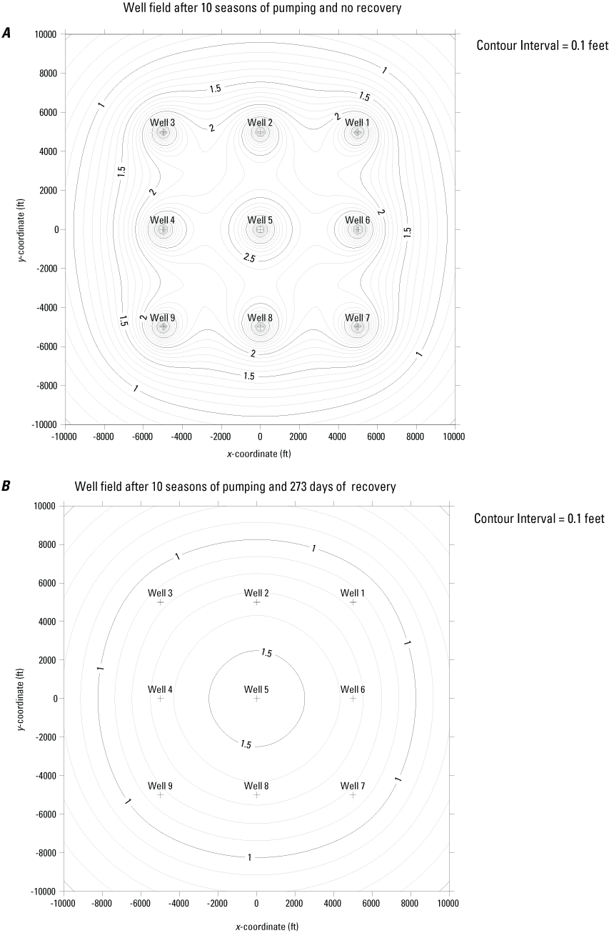
Water table contour maps showing the predicted peak drawdown in a hypothetical well field at the end of 10 irrigation periods. Each irrigation period consists of 92 consecutive days of pumping from nine wells to extract 400 acre-feet of groundwater and is followed by a 273-day non-pumping period to simulate groundwater recovery during the non-growing season of each year. A, Peak drawdown condition following the 10 irrigation periods, before the final recovery period. B, Residual drawdown following 273 days of recovery from condition shown in A. Simulation was done using Forward Solution Wizard in AQTESOLV version 4.5 (Duffield, 2007) and the Neuman method for unconfined aquifers (Neuman, 1974). Contour maps were created using Golden Software Surfer version 19.2.213. ft, feet.
The two forward solutions discussed in this section are based on estimates of aquifer hydraulic properties obtained from a single aquifer test. The actual hydraulic properties of the alluvial aquifer likely vary considerably across the study area. For this reason, there could be substantial differences between the results of a real-world application of the two pumping scenarios and what is predicted by the forward solutions presented here. Actual drawdowns in the three production wells tested by Johnson (1999a) ranged from 11.74 to 14.43 ft after 2 days of pumping at a rate of around 100 gal/min.
Discussion
Groundwater Levels
Groundwater-Level Declines
As described in the “Results” section, a notable decline in measured water levels occurred between the earlier study conducted by Johnson (1999a) and the current study. During this 23-year time span, measured water levels dropped between 5.6 and 12.2 ft in study observation wells. Information to determine what caused the decline in water levels between the two periods is insufficient, but Arizona has been in a drought since 2000. Using hydrological modeling and tree-ring reconstruction for the Southwest, Williams and others (2020) found that the period from 2000 to 2018 was the second driest 19-year period since 800 C.E., exceeded only by the late-1500s megadrought.
As discussed in the “Hydrology and Hydrogeology” section, infiltration of surface-water flow from the Little Colorado River probably provides most recharge to the alluvial aquifer. An analysis of surface-water flow at the Cameron streamgage was conducted to see if it has changed since the Johnson (1999a) study. This is the only streamgage on the Little Colorado River with an adequate continuous record to look at changes in flow from before the Johnson (1999a) study to the present. The streamgage is located more than 60 mi downstream of the study area so the correlation between streamflow at this streamgage and water levels in the alluvial aquifer can only be analyzed in a qualitative sense. Surface-water flow enter the Little Colorado River between the study area and the Cameron streamgage, most notably at Dinnebito and Moenkopi Washes, which are ephemeral where they enter the Little Colorado River but periodically flow from precipitation runoff mainly during the summer and fall. Still, as an index of how drought may have affected flow in the Little Colorado River, the record from the Cameron streamgage is probably informative. The Little Colorado River is ephemeral from the study area to the Cameron streamgage, flowing only in response to runoff from precipitation or snow melt. An analysis was done by comparing the number of days of measurable flow at the Cameron streamgage for the 20 years between the end of the Johnson study and this study (2000–20) and the number of days of measurable flow for the 20 years prior to the Johnson study (1979–99). The analysis found that there were 15 percent more days with flow from 1979 to 1999 than from 2000 to 2020. When the same analysis was done for days with mean discharge greater than 500 ft3/s, it was found there were 42 percent more days with flow above 500 ft3/s during the period from 1979 to 1999 than from 2000 to 2020.
Another interesting aspect of the drop in groundwater levels from the late 1990s to the present is how it should affect potential recharge from the river in the study area. The late 1990s water levels indicate the water table should have been within a few feet of the bottom of the riverbed. This means the river was probably hydraulically connected to the aquifer when it was flowing. Recharge from a hydraulically connected river is usually less than from a river that is not connected. The unsaturated sediment between the riverbed and water table leaves room for storage so more infiltration can take place when there is flow in the river (Lerner and others, 1990). This should provide a buffer resisting the lowering of the water table because recharge will become more efficient as additional storage space becomes available. This makes the decline in water levels since the late 1990s even more remarkable.
It is unclear what role, if any, tamarisk trees played in the water table decline between the two study periods. Tamarisk have been present on the floodplain of the Little Colorado River in the study area since at least the 1940s (Hereford, 1984). No attempt was made to measure the density of tamarisk trees within the study area but review of imagery available through Google Earth showed the area of tree cover on the floodplain in 1997 resembled that of 2019. However, one thing does stand out when comparing imagery from 1997 and 2019: the active stream channel was much wider in 1997 (fig. 20). This is likely the result of a flood in 1993. Imagery available from 1985 and 1997 show the channel widened substantially sometime between those years. The 1993 flood peak of 18,200 ft3/s measured at the Cameron streamgage was the largest peak measured since 1947. Only one peak flow since 1993 has been above 10,000 ft3/s (11,500 ft3/s in 2002) with most peak flows since 1993 being below 5,000 ft3/s.
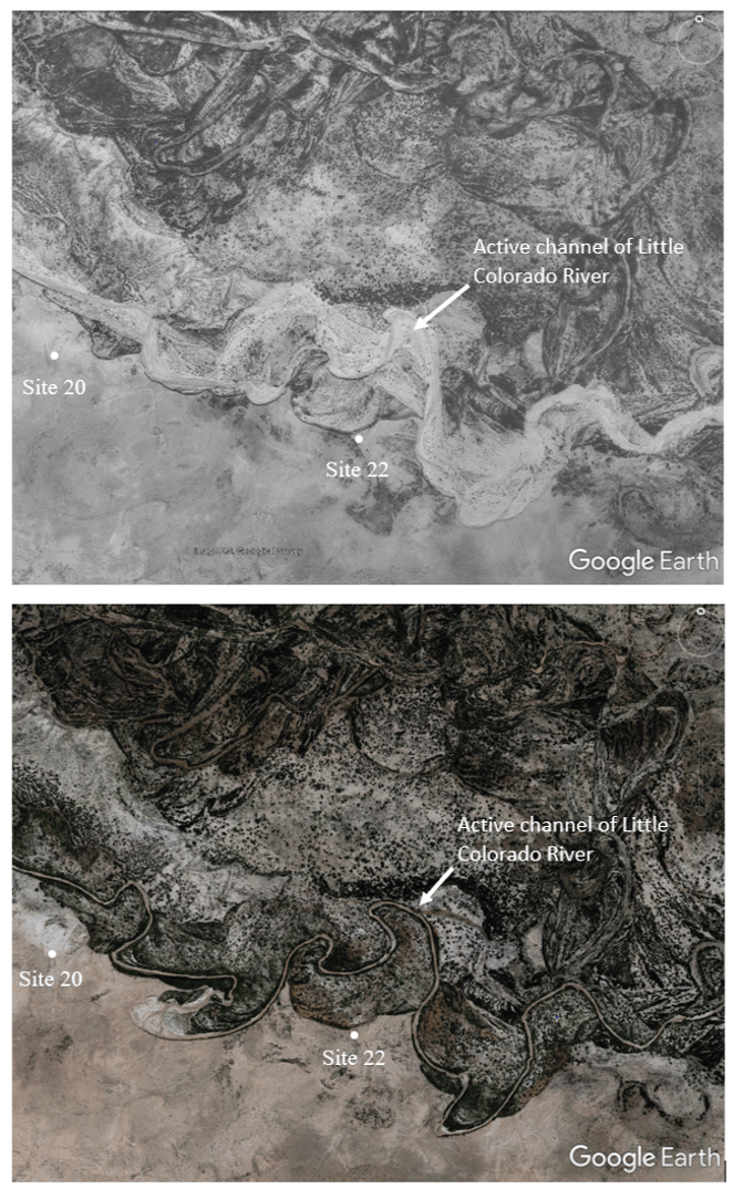
Google Earth images showing area near sites 20 and 22 along the Little Colorado River, Arizona, in 1997 (top) and 2019 (bottom). Active channel of the Little Colorado River appears wider in 1997 image.
Most recharge to the alluvial aquifer from the Little Colorado River likely occurs through the streambed rather than through the floodplain. Even when the floodplain is inundated by water during flood events, water is slow to percolate to the water table owing to the fine-grained nature of floodplain deposits. Figure 21 is an aerial photograph taken 4 weeks after the floodplain was inundated on February 16, 2019. Floodwaters of the Little Colorado River often carry large amounts of clay-sized particles derived from Mesozoic formations in the Painted Desert. Clay-sized particles are deposited in the low energy environment of the floodplain forming a low-permeability mud layer. Much of the water that inundates the floodplain likely either flows back into the main channel without infiltrating or evaporates where it has ponded. For this reason, it is likely that more recharge from the river takes place during periods when the active channel is wider like after the 1993 flood, than it does now when the channel is narrower.
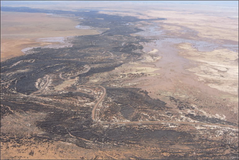
Aerial photograph looking northwest from south end of study area, northeastern Arizona. Ponded water is from a flood that peaked February 16, 2019, on the Little Colorado River. Photograph by Jon Mason, U.S. Geological Survey, March 16, 2019.
Variation in Groundwater Hydraulic Head with Depth
Installation of paired wells to determine if vertical groundwater gradients were present in the alluvial aquifer were delayed owing to the coronavirus pandemic. In the end, only a few groundwater measurements were collected before the study ended. However, the measurements collected still provide valuable insight into the possible presence of vertical gradients within the aquifer. As described in the “Results” section, paired water-level measurements in shallow and deep wells at site 45 indicated that the vertical gradient was either very small in a downward direction or nonexistent when the measurements were made. At site 20 the paired water-level measurements were erratic, possibly because the deep well was completed in an impermeable clay-rich layer. Determining the absence or presence of a vertical groundwater gradient based solely on the differences in water-level elevation within the paired wells was inconclusive at site 20. Nonetheless, the fact that such a thick and impermeable clay-rich layer exists at depth in the aquifer indicates there likely isn’t vertical groundwater flow present between the bedrock and the alluvial aquifer at site 20.
One possible interpretation for this clay-rich layer is that it could be a weathered claystone or siltstone from the Chinle Formation. A qualitative comparison between sediment collected from an outcrop of the Chinle Formation about 5 mi southeast of site 20 and auger cuttings obtained from the clay-rich layer in the well bore of BS-20D, showed the two samples of sediment were very similar. This is a hypothetical interpretation because the two samples might be similar because the clay-rich layer in the well bore was an overbank deposit from the Little Colorado River that was partly derived from weathering of the Chinle Formation. Also, if this layer was a weathered claystone or siltstone from the Chinle Formation it is unlikely that a hollow-stem auger would be able to penetrate it so far.
The possible existence of vertical groundwater gradients has important implications for aquifer recharge and potential sources of high total dissolved solids. One question this study wanted to answer is whether any recharge was occurring to the alluvial aquifer from the underlying bedrock because Johnson (1999b) considered bedrock a possible source for the high total dissolved solids found in the alluvial aquifer. Preliminary results from sites 20 and 45 indicate that vertical groundwater gradients within the alluvial aquifer may be small or nonexistent.
Implications of Groundwater Chemistry for Recharge
The interactions of Little Colorado River surface water with upstream brackish groundwater from the C aquifer are not completely understood and more work is needed to fully comprehend this system’s implications for water chemistry and recharge of the alluvial aquifer. The following discussion on groundwater chemistry and recharge is based on qualitative observations and may require revision when more information becomes available.
The salt sodium chloride is very soluble in water and tends to pass through open flow hydrologic systems rather than becoming concentrated. When expressed in milliequivalents per liter, sodium and chloride both account for more than 50 percent of the cations and anions in water-chemistry samples from the alluvial aquifer (fig. 15). The fact that sodium and chloride are the dominant ions in water-chemistry samples from the alluvial aquifer may provide valuable clues about the aquifer’s recharge.
Johnson (1999b) was confounded by both the high concentrations of total dissolved solids in water-chemistry samples from some alluvial aquifer wells, and by the high variability in concentrations between wells. He concluded that most recharge was occurring from the Little Colorado River, mainly during the spring runoff season, with smaller amounts of recharge coming from the Little Colorado River during the monsoon season and from upstream groundwater inflow and direct infiltration of precipitation. Total dissolved-solids concentrations from 20 water-chemistry samples available from streamgage 09401000, Little Colorado River at Grand Falls, Ariz., ranged from 136 to 1,080 mg/L with a median value of 353 mg/L (USGS, 2022b). Total dissolved-solids concentrations from alluvial aquifer samples collected in 1998 by Johnson (1999b) ranged from 896 to 6,114 mg/L with a median value of 1,310 mg/L, whereas total dissolved-solids concentrations from the nine alluvial aquifer samples collected for this study ranged from 915 to 6,330 mg/L with a median value of 1,370 mg/L (fig. 22).
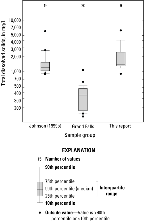
Boxplot of total dissolved-solids concentrations comparing water-chemistry samples collected from the Little Colorado River alluvial aquifer, northeastern Arizona, for this study with samples collected by Johnson (1999b) from the alluvial aquifer and with historical surface-water-chemistry samples available from streamgage 09401000, Little Colorado River at Grand Falls, Arizona. mg/L, milligrams per liter.
Johnson (1999b) postulated that the higher total dissolved solids in the aquifer could be coming from the Moenkopi Formation. He noted that the wells with the highest total dissolved solids were wells that penetrated a small distance into the Moenkopi Formation. There are several incongruities with this hypothesis. Although there are wells developed in the Moenkopi Formation within Arizona, the formation is usually considered an aquitard because it generally consists of thin beds of sandstone with abundant fine-grained beds of siltstone and mudstone. On top of the general low permeability found in the Moenkopi Formation, the wells Johnson (1999b) described have 20- to 40-ft screened intervals, but only penetrate a few feet into the Moenkopi Formation. This would indicate that most water from the wells would come from the more permeable alluvial aquifer limiting the effect that water from the Moenkopi Formation could have on overall total dissolved-solids concentrations. Based on available water-chemistry samples from the USGS NWIS database and collected in Arizona from Moenkopi springs and wells, water from the Moenkopi Formation tends to be of either a mixed water type or of calcium-sulfate and calcium-bicarbonate water types (appendix 2; USGS, 2022b). Only 1 of the 20 Moenkopi Formation samples available had a sodium-chloride water type.
Although there is no obvious source of sodium chloride within the alluvial aquifer itself, there is a known source for sodium chloride upstream along the Little Colorado River in the Three Canyons area southeast of Winslow where Clear Creek, Chevelon Creek, and Jacks Canyon enter the Little Colorado River. Numerous springs issue from the Coconino Sandstone (part of the C aquifer) near the mouths of Clear Creek and Chevelon Canyon that have a sodium-chloride water type with total dissolved-solids concentrations (2,230–3,610 mg/L) that are considered brackish in some instances. The high sodium and chloride concentrations present within the C aquifer in this area are believed to result from the dissolution of evaporite beds, composed primarily of halite, within the Schnebly Hill Formation upgradient from the springs (Mann, 1976). Evidence for this process can be seen several miles to the south of the springs in the form of sinkholes called the McCauley Sinks. Neal and Johnson (2002) describe the McCauley Sinks as a group of about 50 sinkholes developed in the Kaibab Limestone and Coconino Sandstone formed by dissolution of evaporites in the western part of the Holbrook basin, adjacent to Chevelon Canyon (fig. 23). The evaporites originated within an inland sea during the Permian period as part of the Schnebly Hill Formation (Neal and others, 2013), which is part of the C aquifer and hydraulically connected to the Coconino Sandstone in the Holbrook basin.
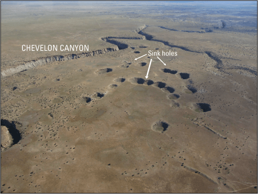
Oblique aerial photograph looking north at McCauley Sinks and Chevelon Canyon, approximately 17 miles southeast of Winslow, Arizona. Photograph by Jon Mason, U.S. Geological Survey, June 27, 2020.
C-aquifer springs in the Three Canyons area support a short reach of perennial flow in the Little Colorado River. Because of the high sodium and chloride concentrations in this water, the flow should contribute sodium and chloride to the alluvial aquifer in the Three Canyons area. The flow also likely deposits salt in the Little Colorado River channel during baseflow conditions through wicking of water upward through alluvial sediments and evaporation. These salts would then be remobilized by the river during higher flow events. A similar phenomenon of springs supplying sodium chloride to a stream was pointed out by Feth and Hem (1963) for the Gila River in Arizona. They reported that the chemical composition of the Gila River is strongly influenced by several hundred tons per day of sodium chloride entering the river by springs issuing from Precambrian quartzite.
Figure 24 shows the relative ionic compositions of water from the alluvial aquifer, Three Canyons area springs, Grand Falls streamgage surface water, and the Moenkopi Formation. Ionic compositions of water from the alluvial aquifer and both Three Canyons area springs and surface water from the Grand Falls streamgage overlap considerably. There is less overlap in ionic composition between water from the alluvial aquifer and from the Moenkopi Formation. This supports the hypothesis that water in the alluvial aquifer largely came from a combination of surface-water flow from the Little Colorado River and groundwater flow influenced by discharge from springs in the Three Canyons area.
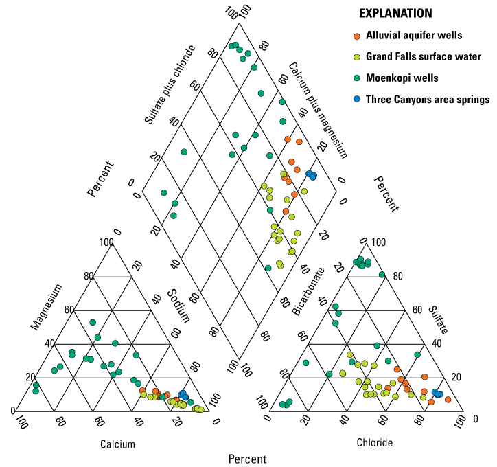
Piper diagram (Piper, 1944) showing the relative ionic compositions of water from the Little Colorado River alluvial aquifer; streamgage 09401000, Little Colorado River at Grand Falls, Arizona; the Moenkopi Formation; and Three Canyons area springs, northeastern Arizona.
Although the ionic composition of alluvial aquifer water is similar to the composition of Little Colorado River surface water sampled at the Grand Falls streamgage, the median concentration of total dissolved solids from alluvial aquifer samples are about 4 to 5 times greater than surface-water-chemistry samples. Two estimations indicate what could be driving total dissolved-solids concentration higher in the alluvial aquifer. First, Reclamation (1999) estimated that only about 15.6 acre-ft of water leaves the study area as groundwater flow downstream each year, and second, Johnson (1999a) estimated evapotranspiration from tamarisk to be about 10,400 acre-ft/yr in the study area. Evapotranspiration of groundwater has the potential to increase the total dissolved-solids concentrations because it removes water while generally leaving behind dissolved solids. This mechanism would likely be especially effective because the amount of groundwater available to flush dissolved solids downstream of the study area is believed to be relatively small (~15.6 acre-ft/yr). However, the effect of withdrawal by tamarisk on groundwater chemistry is not as straightforward because tamarisk is known to extract salt from groundwater and can both sequester salt in its tissues and secrete salt from its leaves. Numerous studies have been conducted to assess the effect tamarisk have on the salinity of soil, but the authors are unaware of any studies that directly assess the effects tamarisk have on groundwater salinity.
Implications of Groundwater Chemistry for Crop Irrigation
Although water is necessary to grow and sustain plants, the chemical and physical properties of water used by plants also can have adverse effects on plant health. High salinity, sodium-adsorption ratio (SAR), and concentrations of specific ions in irrigation water can present hazards to plant health (Ayers, 1977).
Salinity Hazard
Table 8, adapted from Ayers (1977), shows the potential yield reduction from saline waters for common irrigated crops. Salinity in table 8 is expressed as the specific conductance of irrigation water in microsiemens per centimeter (µS/cm). The crops in table 8 are listed in descending order from the most saline-resistant crops at the top to least resistant at the bottom. The specific conductance of water from wells measured for this study ranged from 1,590 to 10,300 µS/cm. According to table 8 this level of salinity in irrigation water could have a negative effect on many of the crops listed. Table 8 indicates that corn, a common crop grown on the Navajo Nation, likely would be minimally affected if salinity were near the lower end of what was measured in observation wells but could be seriously affected by irrigation water near the higher end of the salinity range found in the wells.
Table 8.
Potential yield reduction from using saline water for selected irrigated crops.[Adapted from Ayers (1977). %, percent; µS/cm, microsiemens per centimeter.]
Buildup of salinity in the soil is another hazard associated with crop irrigation. Much of the water applied during irrigation is removed from the soil to meet crop evapotranspiration demand while leaving behind most of the salt. To prevent damaging salinity buildup in soil, sufficient irrigation water must be applied to leach salt from the root zone. The portion of water that passes through the rooting depth is called the leaching fraction. If the leaching fraction is too small, damaging salt build up will occur in the soil (Ayers and Westcot, 1985). This issue is exacerbated in soils with low permeability. In low-permeability soils additional mitigation may be required such as installing tile drains to keep the water table from invading the root zone (Hem, 1985).
Sodium-Adsorption Ratio (SAR) Hazard
SAR, as defined by the U.S. Salinity Laboratory (1954), is expressed as
whereNa+
is sodium in milliequivalents
Ca2+
is calcium in milliequivalents
Mg2+
is magnesium in milliequivalents
SAR is used to predict the degree to which irrigation water enters into cation-exchange reactions in the soil (Hem, 1985). High SAR values can make water unsuitable for irrigation use because it can lead to sodium replacing adsorbed calcium and magnesium in soils, resulting in damage to soil structure and lowering soil permeability. Figure 25 shows the potential combined effect of SAR and specific conductance on soil infiltration. Except for water with low specific conductance (<200 µS/cm), the effect of SAR on soil infiltration is generally reduced as the specific conductance of irrigation water increases. Results from 8 of the observation wells sampled for this study are plotted on figure 25 and indicate that water from 1 well (BS-17) might have a slight to moderate effect on soil permeability. The SAR result for water from well BS-23 (16.0) is not shown on the figure because the specific conductance value of this sample (10,300 µS/cm) is greater than the scale used for the x-axis of the plot. Lower specific conductance is generally better for plant health, but because sodium is the dominant cation in the alluvial aquifer, lower specific conductance could lead to reduced soil permeability.
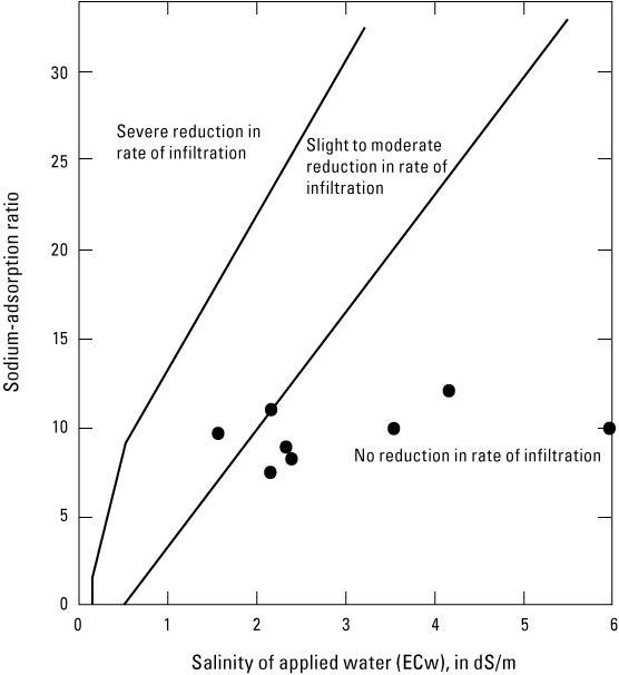
Plot of relative rate of water infiltration as affected by salinity and sodium-adsorption ratio with results from eight Little Colorado River alluvial aquifer wells sampled for this study, northeastern Arizona. Modified from Ayers and Westcot (1985). dS/m, decisiemens per meter.
Specific-Ion Toxicity
The ions boron and chloride are essential to plant growth at very low concentrations, but at greater concentrations they can become toxic. Sodium is not essential for plant growth and is known to have a toxic effect on the growth of certain sensitive crops even at low concentrations.
Boron can begin to be a hazard for plants when its concentration in irrigation water exceeds 500 µg/L (Ayers, 1977). Boron concentrations in water sampled from observation wells in the alluvial aquifer for this study were all below the plant-hazard level ranging from 219 to 381 µg/L.
Both sodium and chloride in irrigation water can cause damage to tree crops through root absorption. Sodium can be hazardous when the SAR is greater than 3 and chloride begins to be hazardous to tree crops at concentrations greater than 142 mg/L (Ayers, 1977). Most annual crops are not as sensitive to root absorption and the salinity tolerance in table 8 can be used as a guide to assess effects related to root absorption. When sprinkler irrigation is used, salt-sensitive crops may be affected by foliar absorption if sodium concentrations are greater than 69 mg/L and chloride concentrations are greater than 106 mg/L (Ayers, 1977). The SAR in water from observation wells completed in the alluvial aquifer and sampled for this study ranged from 7.68 to 16.0, whereas concentrations of sodium and chloride ranged from 277 to 1,520 and 297 to 3,230 mg/L, respectively.
Implications of Well-Field Pumping Scenarios for Crop Irrigation
Results from the well-field pumping scenarios conducted for this study indicate that groundwater from the alluvial aquifer could be used for irrigated agriculture, but the economic sustainability of this water use may be marginal. Although the alluvial aquifer contains a relatively large amount of groundwater compared to the water needs of the irrigated agriculture purposed in this study (100 acres of land), the inability of groundwater to move through the aquifer at a rate suitable for crop irrigation would make the economics of this water use challenging. The pumping scenarios show that multiple irrigation wells spaced thousands of feet apart would be required to irrigate just 100 acres of land.
Conclusions
The Little Colorado River alluvial aquifer near Leupp, Arizona (fig. 1), was investigated as a possible source of irrigation water for the Leupp and Birdsprings Chapters of the Navajo Nation. Groundwater quality in the alluvial aquifer appears to be negatively affected by the aggregated effects of discharge from C-aquifer springs with poor water quality upstream of the study area and the large amount of evapotranspiration that occurs from floodplain vegetation within the study area. The water chemistry of groundwater from the aquifer was analyzed for salinity hazard, sodium-adsorption hazard, and specific-ion toxicity. The salinity hazard was high enough in most areas that it could negatively affect salt-sensitive crops. Further, salt buildup in the soil as a result of using irrigation water with high total dissolved-solids concentrations may eventually require some form of mitigation such as additional water application to leach salt from the root zone and use of tile drains. The sodium-adsorption hazard of groundwater from the alluvial aquifer was found to be low and specific-ion toxicity was low as well, except for possible ion toxicity from sodium and chloride for tree crops.
The well-field pumping scenarios conducted for this study demonstrated that using groundwater from the alluvial aquifer for irrigated agriculture is theoretically possible. However, the pumping scenarios showed that multiple irrigation wells spaced thousands of feet apart would be required to irrigate just 100 acres of land, making the economic feasibility of this water use uncertain. Given the additional uncertainties of how water chemistry of the alluvial aquifer might affect crop yields, it may be prudent to conduct a pilot study using just 1 or 2 wells to irrigate a small plot of land and assess how desired crops and the soil are affected by using alluvial aquifer water for irrigation.
References Cited
Beisner, K.R., Tillman, F.D., Anderson, J.R., Antweiler, R.C., and Bills, D.J., 2017, Geochemical characterization of groundwater discharging from springs north of the Grand Canyon, Arizona, 2009–2016: U.S. Geological Survey Scientific Investigations Report 2017–5068, 58 p., https://doi.org/10.3133/sir20175068.
Billingsley, G.H., Block, D., and Hiza Redsteer, M., 2013, Geologic map of the Winslow 30′ × 60′ quadrangle, Coconino and Navajo Counties, northern Arizona: U.S. Geological Survey Scientific Investigations Map 3247, pamphlet 25 p., 3 sheets, scale 1:50,000, and GIS data, https://pubs.usgs.gov/sim/3247/.
Blasch, K., Ferré, P.A., Hoffmann, J., Pool, D., Bailey, M., and Cordova, J., 2004, Processes controlling recharge beneath ephemeral streams in southern Arizona, in Hogan, J.F., Phillips, F.M., and Scanlon, B.R., eds., Groundwater Recharge in a Desert Environment—The Southwestern United States, Water Science and Application 9: Washington, DC, American Geophysical Union, p. 69–76.
Duffield, G.M., 2007, AQTESOLV for Windows Version 4.5 User’s Guide: Reston, Va., HydroSOLVE, Incorporated, accessed December 2020 at https://hwbdocuments.env.nm.gov/Los%20Alamos%20National%20Labs/General/37764.pdf.
Duffield, W., Riggs, N., Kaufman, D., Champion, D., Fenton, C., Forman, S., McIntosh, W., Hereford, R., Plescia, J., and Ort, M., 2006, Multiple constraints on the age of a Pleistocene lava dam across the Little Colorado River at Grand Falls, Arizona: Geological Society of America Bulletin, v. 118, no. 3-4, p. 421–429.
Frisvold, G.B., 2015, Developing Sustainability Metrics for Water Use in Arizona Small Grain Production: Tucson, Ariz., Department of Agricultural and Resource Economics, University of Arizona, accessed January 13, 2021, at https://agriculture.az.gov/sites/default/files/documents/Developing%20Sustainability%20Metrics%20for%20Water%20Use%20in%20Arizona%20Small%20Grain%20Pr oduction.pdf.
Goodrich, D.C., Williams, D.G., Unkrich, C.L., Hogan, J.F., Scott, R.L., Hultine, K.R., Pool, D., Coes, A.L., and Miller, S., 2004, Comparison of methods to estimate ephemeral channel recharge, Walnut Gulch, San Pedro River Basin, Arizona, in Hogan, J.F., Phillips, F.M., and Scanlon, B.R., eds., Groundwater Recharge in a Desert Environment—The Southwestern United States, Water Science and Application 9: Washington, D.C., American Geophysical Union, p. 77–99.
GRAV-D Team, 2017, GRAV-D General Airborne Gravity Data User Manual (ver. 2.1) (T. Damiani, M. Youngman, and J. Johnson, eds.): National Geodetic Survey, accessed January 12, 2022, at https://www.ngs.noaa.gov/GRAV-D/data_products.shtml.
GRAV-D Team, 2018, Gravity for the redefinition of the American Vertical Datum (GRAV-D) Project, Airborne Gravity Data; Block MS04: National Geodetic Survey data, accessed January 12, 2022, at https://www.ngs.noaa.gov/GRAV-D/data_ms04.shtml.
Hinze, W.J., Aiken, C., Brozena, J., Coakley, B., Dater, D., Flanagan, G., Forsberg, R., Hildenbrand, T., Keller, G.R., Kellogg, J., Kucks, R., Lee, X., Mainville, A., Morin, R., Pilkington, M., Plouff, D., Ravat, D., Roman, D., Urrutia-Fucugauchi, J., Véronneau, M., Webring, M., and Winester, D., 2005, New standards for reducing gravity data—The North American gravity database: Geophysics, v. 70, no. 4, p. J25–J32.
Kennedy, J., 2020, GSadjust v1.0: U.S. Geological Survey software release, https://doi.org/10.5066/P9YEIOU8.
Kennedy, J.R., 2023, Gravity data along the Little Colorado River near Leupp, Arizona: U.S. Geological Survey data release, https://doi.org/10.5066/P9E6AXVJ.
Kennedy, J.R., Pool, D.R., and Carruth, R.L., 2021, Procedures for field data collection, processing, quality assurance and quality control, and archiving of relative- and absolute-gravity surveys: U.S. Geological Survey Techniques and Methods, book 2, chap. D4, 50 p., https://doi.org/10.3133/tm2D4.
Macy, J.P., and Mason, J.P., 2023, Electrical resistivity tomography data along the Little Colorado River near Leupp, AZ 2019: U.S. Geological Survey data release, https://doi.org/10.5066/P9TNW6SD.
Moore, R.B., and Wolf, E.W., 1987, Geologic map of the east part of the San Francisco Volcanic Field, north-central Arizona: U.S. Geological Survey Miscellaneous Field Studies Map 1960, 46 p., 2 plates, scale 1:50,000, available at https://pubs.er.usgs.gov/publication/mf1960.
National Oceanic and Atmospheric Administration, 2020, U.S. climate normal quick access: National Centers for Environmental Information, National Oceanic and Atmospheric Administration, accessed March 13, 2020, at https://www.ncei.noaa.gov/access/us-climate-normals/.
Neal, J.T., Johnson, K.S., and Lindberg, P., 2013, Variations in evaporite karst in the Holbrook basin, Arizona: in Land, L., Doctor, D.H., and Stephenson, J.B., eds., Sinkholes and the engineering and environmental impacts of karst, Proceedings of the Thirteenth Multidisciplinary Conference: Carlsbad, N. Mex., National Cave and Karst Research Institute, p. 177–186.
PRISM Climate Group, 2020, PRISM climate data: Northwest Alliance for Computational Science and Engineering, Oregon State University, accessed March 13, 2020, at http://prism.oregonstate.edu.
Révész, K., and Coplen, T.B., 2008a, Determination of the δ2H/1H, of water—RSIL lab code 1574: U.S. Geological Survey Techniques and Methods, book 10, chap. C1, 27 p., accessed January 2021 at https://pubs.usgs.gov/tm/2007/tm10c1/.
Révész, K., and Coplen, T.B., 2008b, Determination of the δ18O/16O, of water—RSIL lab code 489: U.S. Geological Survey Techniques and Methods, book 10, chap. C2, 28 p., accessed January 2021 at https://pubs.usgs.gov/tm/2007/tm10c2/.
Seequent, 2022, GM-SYS: Seequent software, https://www.seequent.com/products-solutions/geosoft-oasis-montaj/gm-sys/.
Struzeski, T.M., DeGiacomo, W.J., and Zayhowski, E.J., 1996, Methods of analysis by the U.S. Geological Survey National Water Quality Laboratory—Determination of dissolved aluminum and boron in water by inductively coupled plasma-atomic emission spectrometry: U.S. Geological Survey Open-File Report 96–149, 17 p.
Sweeney, R.E., and Hill, P.L., 2001, Arizona aeromagnetic and gravity maps and data—A web site for distribution of data (ver. 1.0): U.S. Geological Survey Open-File Report 01-0081, accessed August 20, 2018, at https://pubs.usgs.gov/of/2001/ofr-01-0081/html/az_iso.htm.
Thatcher, L.L., Janzer, V.J., and Edwards, K.W., 1977, Methods for determination of radioactive substances in water and fluvial sediments: U.S. Geological Survey Techniques of Water-Resources Investigations, book 5, chap. A5, accessed February 27, 2021, at https://doi.org/10.3133/ofr76560.
U.S. Environmental Protection Agency [EPA], 2023a, National primary drinking water regulations: U.S. Environmental Protection Agency web page, accessed January 2023 at https://www.epa.gov/ground-water-and-drinking-water/national-primary-drinking-water-regulations.
U.S. Environmental Protection Agency [EPA], 2023b, Secondary drinking water standards—Guidance for Nuisance Chemicals: U.S. Environmental Protection Agency web page, accessed January 2023 at https://www.epa.gov/sdwa/secondary-drinking-water-standards-guidance-nuisance-chemicals.
U.S. Geological Survey [USGS], 2022a, 3D Elevation Program 1/3 arc-second Digital Elevation model: U.S. Geological Survey data, accessed January 11, 2022, at https://apps.nationalmap.gov/downloader/.
U.S. Geological Survey [USGS], 2022b, USGS water data for the Nation: U.S. Geological Survey National Water Information System database, accessed November 2021 at https://doi.org/10.5066/F7P55KJN.
U.S. Geological Survey [USGS], [variously dated], National field manual for the collection of water-quality data: U.S. Geological Survey Techniques and Methods of Water-Resources Investigations, book 9, chaps. A1–A10, accessed December 2019 at https://pubs.water.usgs.gov/twri9A.
Western Regional Climate Center, 2022a, Leupp, Arizona (024872)—Period of record monthly climate summary: Western Regional Climate Center database, accessed May 4, 2022, at https://wrcc.dri.edu/cgi-bin/cliMAIN.pl?az4872.
Western Regional Climate Center, 2022b, Leupp, Arizona (024872)—Period of record general climate summary, Temperature: Western Regional Climate Center database, accessed May 4, 2022, at https://wrcc.dri.edu/cgi-bin/cliGCStT.pl?az4872.
Western Regional Climate Center, 2022c, Leupp, Arizona (024872)—Total of snowfall (inches): Western Regional Climate Center database, accessed May 4, 2022, at https://wrcc.dri.edu/WRCCWrappers.py?sodxtrmts+024872+por+por+snow+none+msum+5+07+F.
Western Regional Climate Center, 2022d, Winslow Municipal Airport, Arizona (029439)—Period of record general climate summary, Temperature: Western Regional Climate Center database, accessed May 4, 2022, at https://wrcc.dri.edu/cgi-bin/cliGCStT.pl?az9439.
Western Regional Climate Center, 2022e, Winslow Municipal Airport, Arizona (029439)—Total of snowfall (inches): Western Regional Climate Center database, accessed May 4, 2022, https://wrcc.dri.edu/WRCCWrappers.py?sodxtrmts+029439+por+por+snow+none+msum+5+07+F.
Williams, P.A., Cook, E.R., Smerdon, J.E., Cook, B.I., Abatzoglou, J.T., Bolles, K., Baek, S.H., Badger, A.M., and Livneh, B., 2020, Large contribution from anthropogenic warming to an emerging North American megadrought: Science, v. 368, no. 6488, p. 314–318, https://doi.org/10.1126/science.aaz9600.
Appendix 1. Water-chemistry sample results from monitoring wells, Little Colorado River alluvial aquifer, northeastern Arizona
Appendix 2. Major ion chemistry results of water samples collected from springs and wells in the Moenkopi Formation in Arizona
Conversion Factors
U.S. customary units to International System of Units
International System of Units to U.S. customary units
Temperature in degrees Celsius (°C) may be converted to degrees Fahrenheit (°F) as follows:
°F = (1.8 × °C) + 32.
Temperature in degrees Fahrenheit (°F) may be converted to degrees Celsius (°C) as follows:
°C = (°F – 32) / 1.8.
Datum
Vertical coordinate information is referenced to the North American Vertical Datum of 1988 (NAVD 88).
Horizontal coordinate information is referenced to the North American Datum of 1983 (NAD 83).
Supplemental Information
Specific conductance is given in microsiemens per centimeter at 25 degrees Celsius (µS/cm at 25 °C).
Concentrations of chemical constituents in water are given in either milligrams per liter (mg/L) or micrograms per liter (µg/L).
Activities for radioactive constituents in water are given in picocuries per liter (pCi/L).
Abbreviations
BIA
Bureau of Indian Affairs
BS
Birdsprings
C aquifer
Coconino aquifer
CBA
complete Bouguer anomaly
D
deep well
DIC
dissolved inorganic carbon
EPA
U.S. Environmental Protection Agency
ERT
electrical resistivity tomography
GPS
Global Positioning System
GRS80
geodetic reference system of 1980
MB
microbasin
MCL
maximum contaminant level
NOSAMS
National Ocean Sciences Accelerator Mass Spectrometry
NWQL
National Water Quality Laboratory
NWIS
National Water Information System
P
production well
PVC
polyvinyl chloride
QC
quality control
Reclamation
Bureau of Reclamation
S
shallow well
SAR
sodium-adsorption ratio
SMCL
secondary maximum contaminant level
TAF
total annual flow
USGS
U.S. Geological Survey
Moffett Field Publishing Service Center, California
Manuscript approved for publication April 23, 2023
Edited by Regan Austin
Layout and design by Kimber Petersen
Disclaimers
Any use of trade, firm, or product names is for descriptive purposes only and does not imply endorsement by the U.S. Government.
Although this information product, for the most part, is in the public domain, it also may contain copyrighted materials as noted in the text. Permission to reproduce copyrighted items must be secured from the copyright owner.
Suggested Citation
Mason, J.P., Kennedy, J.R., Macy, J.P., and Gungle, B., 2023, Hydrologic framework and characterization of the Little Colorado River alluvial aquifer near Leupp, Arizona: U.S. Geological Survey Scientific Investigations Report 2023–5052, 40 p., https://doi.org/10.3133/sir20235052.
ISSN: 2328-0328 (online)
Study Area
| Publication type | Report |
|---|---|
| Publication Subtype | USGS Numbered Series |
| Title | Hydrologic framework and characterization of the Little Colorado River alluvial aquifer near Leupp, Arizona |
| Series title | Scientific Investigations Report |
| Series number | 2023-5052 |
| DOI | 10.3133/sir20235052 |
| Publication Date | June 30, 2023 |
| Year Published | 2023 |
| Language | English |
| Publisher | U.S. Geological Survey |
| Publisher location | Reston, VA |
| Contributing office(s) | Arizona Water Science Center |
| Description | Report: ix, 40 p.; 2 Data Releases; 2 Appendix |
| Country | United States |
| State | Arizona |
| Other Geospatial | Little Colorado River Alluvial Aquifer |