Techniques for estimating the magnitude and frequency of peak flows on small streams in Minnesota, excluding the Rainy River Basin, based on data through water year 2019

Christopher A. Sanocki; Sara B. Levin

doi:10.3133/sir20235079

Techniques for Estimating the Magnitude and Frequency of Peak Flows on Small Streams in Minnesota, Excluding the Rainy River Basin, Based on Data Through Water Year 2019

Scientific Investigations Report 2023-5079

Prepared in cooperation with the Minnesota Department of Transportation

By: Christopher A. Sanocki and Sara B. Levin

https://doi.org/10.3133/sir20235079

Links

Document: Report (3.6 MB pdf) , HTML , XML
Dataset: USGS National Water Information System database —USGS water data for the Nation
Data Releases:
- USGS data release —Model archive of regional flood frequency equations for Minnesota streams
- USGS data release
Download citation as: RIS | Dublin Core

Abstract

Annual peak-flow data collected at U.S. Geological Survey streamgages in Minnesota and adjacent areas of neighboring states of Iowa and South Dakota were analyzed to develop and update regional regression equations that can be used to estimate the magnitude and frequency of peak streamflow for ungaged streams in Minnesota, excluding the Lake of the Woods-Rainy River Basin upstream from Kenora, Ontario, Canada. Hydraulic engineers use peak-flow frequency estimates to inform designs of bridges, culverts, and dams, and water managers use the estimates for regulation and planning activities. Peak-flow estimates are provided for the 66.7-, 50-, 20-, 10-, 4-, 2-, 1-, and 0.2-percent annual exceedance probabilities (AEPs), which are equivalent to annual flood-frequency recurrence intervals of 1.5-, 2-, 5-, 10-, 25-, 50-, 100-, and 500-years, respectively. The estimates were computed by applying the expected moments algorithm to fit a Pearson Type III distribution to the logarithms of annual peak flows for 298 streamgages based on annual peak-flow data collected through water year 2019. The study area is represented by six hydrologic regions delineated on the basis of a pattern of residuals of statewide regressions, using basin characteristics such as drainage area, main-channel slope, lake area, storage area, and mean annual runoff as explanatory variables. The concept and principles of hydrologic landscape units was used to validate the regions. Residual analysis of the regional regression equations was used to subsequently develop equations relating the peak flow estimates for selected AEPs using 17 characteristics tested as explanatory variables in the regression analysis.

The equations developed in this study can be used to produce AEPs within the six regions and to update equations developed in earlier, similar studies in Minnesota. Furthermore, updating the equations in StreamStats, a web-based geographic information system tool developed by the U.S. Geological Survey, will allow hydraulic engineers and water managers to obtain AEPs and basin characteristics for user-selected locations on streams through an interactive map.

Introduction

Estimates of the magnitude and frequency of peak streamflow (flow) at ungaged locations along streams are needed for the management of water within the State of Minnesota, United States. Peak flows for a stream are expected to occur at a given recurrence interval more precisely expressed as an annual exceedance probability (AEP). For example, 1- and 0.2-percent AEPs represent a 1 in 100 and 1 in 500 chance of being equaled or exceeded in any given year, and have average recurrence intervals of 100 and 500 years, respectively. Peak-flow frequency estimates are essential for engineering bridges, dams, and levees; flood-plain mapping (Federal Emergency Management Agency, 2002); estimating scour at bridges (Fischer, 1995; Arneson and others, 2012); and evaluating the effect of streamflow on high-priority environmental and water-management challenges. Therefore, where long-term streamflow data are not available, that is, at ungaged locations, statistical techniques are needed to estimate peak flow associated with specified AEPs. To address that need, the U.S. Geological Survey (USGS), in cooperation with the Minnesota Department of Transportation, analyzed streamflow data collected through September 2019 to develop equations to estimate the magnitude and frequency of peak flows at ungaged sites in Minnesota.

Annual peak-flow data from 298 streamgages operated by the USGS were used to develop statistical equations to estimate AEPs for ungaged locations. The equations were developed by using a regression analysis to statistically relate AEPs to basin characteristics that are potential explanatory variables for flow at selected streamgages within Minnesota. The AEPs computed for streamgages can change as additional annual peak-flow data become available. Furthermore, the statistics become more reliable as additional data are collected and used in the computations.

Purpose and Scope

This report presents (1) updated regression models for the prediction of AEPD at locations without streamgages in six hydrologic regions in Minnesota, excluding the binational (United States and Canada) region B1 defined by Sanocki and others (2019), based on explanatory variables; and (2) the 66.7-, 50-, 20-, 10-, 4-, 2-, 1-, and 0.2-percent AEPD for 298 streamgages used in the development of regression equations on the basis of streamflow data collected through USGS water year 2019.

Regional regression equations for estimating the magnitude and frequency of peak-flows at ungaged sites are described in this report. The data used in this analysis were collected from streams that were unaffected, or only minimally affected, by urban development; therefore, the application of the regression equations developed and presented here in analyses of streamflow in dense urban settings is not recommended. Data from streamgages with drainage areas greater than 3,000 square miles were not included in this analysis because of the likelihood of flow regulation on rivers of that size. Data from streamgages for which peak flows were affected by controlled storage or regulated releases also were excluded from this analysis. All data are available in Levin (2023) and the USGS National Water Information System database (USGS, 2019).

Previous Studies

Previous studies of peak flow in Minnesota, including those by Prior (1949), Prior and Hess (1961), Wiitala (1965), Patterson and Gamble (1968), Guetzkow (1977), Jacques and Lorenz (1987), Lorenz and others (1997, 2010), Kessler and others (2013), Ziegeweid and others (2015), Lorenz and Ziegeweid (2016), and Sanocki and others (2019), have provided peak-flow data for selected streamgages and methods for estimating AEPDs at ungaged sites in Minnesota. Analysis of annual peak-flow values reported in these studies, which used the Log Pearson Type III method of analysis (Guetzkow, 1977), may not have included information about historical floods that occurred before the systematic collection of data, and the period of record for many streams was very short from the standpoint of flood history. Guetzkow’s (1977) analysis included data for most of the long-term record stations with low annual peaks from the 1930s drought, and relatively high annual peaks from the 1950s and 1960s. Historical flood information was incorporated into the analyses of subsequent studies. Jacques and Lorenz (1987) used fewer regions than Guetzkow (1977), which resulted in larger standard errors of estimate for the regional equations.

Lorenz (1997) generated station skews for 267 long-term streamgages and produced a generalized skew map. Lorenz and others (2010) also used hydrologic landscape units (Winter, 2001; Wolock and others, 2004) to validate and update hydrologic regions for Minnesota. Eash and others (2013) generated AEPDs for 518 streamgages in Iowa and 50 miles beyond the State’s borders. Sanocki and others (2019) produced the first USGS bi-national peak flow report, which combined the United States and Canadian parts of the Rainy River Basin, thereby creating region B1 from the northern part of Minnesota hydrologic region B (Lorenz and others, 2010) with the Canadian part of the Rainy River Basin, which is characterized by surficial bedrock, lakes, and wetlands (fig. 1).

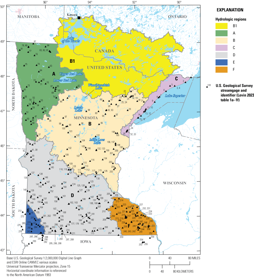
Streamgages are scattered throughout the regions. — Figure 1.
Streamgages used to estimate peak-flow frequencies and magnitudes for Minnesota hydrologic regions A, B, C, D, E, and F.

Description of Study Area

The study area (fig. 1) includes the entire State of Minnesota except for region B1, the Rainy River Basin, which is described in Sanocki and others (2019). Seven hydrologic regions in Minnesota were defined by Lorenz and others (2010) and by Sanocki and others (2019; fig. 1). Region A is one of the most heterogeneous hydrologic regions in the State and has low and moderate slopes along drainage boundaries; it consists primarily of the Red River Basin, which flows north into Canada. Region B is dominated by sandy areas with various slopes and flat expanses of the upper Mississippi River headwaters. Region B1, the binational Rainy River Basin, is characterized by surficial bedrock and thousands of large and small lakes and wetlands. Regions C and F consist of a mix of moderate and high slopes. Region C consists of surficial bedrock sloping to Lake Superior, and Region F is part of the driftless area that was not affected by Pleistocene-era glaciers. Region D is composed of low and moderate slopes next to the upper reaches of the Minnesota River, and material of relatively low sand content in upland areas along the lower part of the river. Region E, in southwestern Minnesota, was separated from region D; although the regions D and E seem similar in figure 3 of Lorenz and others (2010, region E was separated because of distinct drainage pattern differences as shown in figure 2 (Buto and Anderson, 2020).

Streamgages included in this study were assigned a map number, and data associated with each map number (streamgage) are in Levin (2023, tables 1a–1f). The tables include hydrologic, basin, and climatic characteristics and peak-flow frequency discharges for streamgages from which data were used in the regional regression analysis for Minnesota and the neighboring States of Iowa and South Dakota.

Study Methods

The final regression equations were selected based on minimizing values of the standard model error and the standard error of prediction while maximizing values of the pseudo coefficient of determination (R²), followed by examination of regression residuals. Data for 298 active and inactive streamgages in the States of Iowa, Minnesota, and South Dakota, excluding streamgages within the Rainy River Basin, were used in this report (fig. 1; Levin, 2023, tables 1a–1f). Selected streamgages met the following criteria: (1) at least 10 complete water years of reported annual peak flow data were available (England and others, 2019); (2) flow was unaffected by regulation, diversion, or urbanization; and (3) drainage area was less than 3,000 square miles. Geographic information system (GIS) software was used to calculate 17 basin characteristics as potential explanatory variables in the regression analyses.

Techniques for Estimating Peak-Flow Frequency

This section describes the techniques, methods, and computations of the analysis of peak-flow frequency at selected streamgages in Minnesota and the neighboring States of Iowa and South Dakota. The methods and analyses that were required to develop the techniques for estimating peak-flow data on small ungaged streams are described. This section also presents preliminary computations of basin characteristics required for regression analysis.

Peak-Flow Data

Streamflow records selected for analysis in this study consisted of unregulated annual peak-flow data of at least 10 years (Interagency Advisory Committee on Water Data, 1982) through water year 2019 from streamgages in Minnesota and the neighboring states of Iowa and South Dakota. The streamgages selected included 283 from Minnesota, 11 from Iowa, and 4 from South Dakota. The Minnesota peak-flow data were obtained from the USGS National Water Information System peak-flow file (USGS, 2019). Minnesota streamgages used in this study included those with continuous record that documented daily streamflow and partial-record crest-stage streamgages that documented only annual peak flow. These streamgages were verified for completeness of record by investigating gaps in data, historical floods, and potentially influential low flows as described in England and others (2019). Many of the streamgages were seasonal partial record and only operated for part of the year, mainly March through December. The annual peak flow for Minnesota streamgages consisted of the maximum instantaneous discharge for the water year.

Frequency Analysis of Annual Peak-Flow Data at Selected Streamgages

Peak-flow frequency analysis is a statistical technique used to estimate floods associated with known exceedance probabilities (Williams-Sether, 2015). Exceedance probability is the chance or likelihood that a given flow of specific magnitude will be equaled or exceeded in any 1-year period. Exceedance probabilities formerly were reported as flood recurrence intervals expressed in years. For example, a flood magnitude that has a 1-percent chance (exceedance probability=0.01) of being exceeded during any year is expected to be exceeded on average once during any 100-year period (recurrence interval). Percent exceedance probability is the inverse of the recurrence interval multiplied by 100. Although the exceedance probability is an estimate of the likelihood in any 1-year period, more than one flood discharge with a specific magnitude and exceedance probability could happen in the same 1-year period.

Peak-flow frequency estimates are computed by fitting a log-Pearson type 3 distribution to the logarithms (base 10) of the annual peak flows as described in Bulletin 17C (England and others, 2019). The peak-flow frequency estimates in this report were computed using the expected moments algorithm (EMA) with the multiple Grubbs-Beck (MGB; Grubbs and Beck, 1972) test option in the USGS program PeakFQ, version 7.3 (Flynn and others, 2006; Veilleux and others, 2014). EMA addresses several methodological concerns identified in Bulletin 17B (Interagency Advisory Committee on Water Data, 1982) while retaining the essential structure and moments-based approach of the existing Bulletin 17C procedures. Specifically, the EMA method can incorporate censored or interval data into the analysis. Censored data can occur when an annual peak flow falls below a known threshold such as the lowest depth of a crest-stage streamgage. EMA can also incorporate historical flood data or paleo data (geologic or botanical evidence of past floods before the human record), which may not be known precisely but can be described as a range of possible values.

Unlike Bulletin 17B, which recognizes two categories of data—systematic peaks (annual peaks observed in the course of systematic streamgaging at the station) and historical peaks (records of floods that occurred outside the period of regular streamgaging)—EMA uses a more general description of flood information from the historical period that includes systematic and historical peaks.

The MGB test (Grubbs and Beck, 1972) is recommended by Bulletin 17C to detect low outliers in flood-frequency analysis. As described by Cohn and others (2013), the MGB test is a generalization of the Grubbs-Beck method that allows for a standard procedure for identifying multiple potentially influential low flows (PILFs). In flood-frequency analysis, PILFs are annual peaks that meet three criteria: (1) their magnitude is much smaller than the flood quantile of interest; (2) they are below a statistically significant break in the flood-frequency data plot; and (3) they have excessive affect on the estimated frequency of large floods. When an observation is identified as a PILF, all values smaller than that flood are also categorized as PILFs. Identifying PILFs and recording them as censored peaks can greatly improve estimator robustness with little or no loss of efficiency. Thus, the use of the MGB test can improve the fit of the small AEPs while minimizing lack of fit caused by unimportant PILFs in an annual peak series (Cohn and others, 2013; Veilleux and others, 2014).

Procedures in Bulletin 17B recommend the use of a skew coefficient that is based on the skew of the log series of the period of record (commonly termed the “station skew”) weighted with a generalized, or regional, skew coefficient. The weighting is based on the length of the period of record and the estimated standard error for the method used to determine the generalized skew coefficient. Skew coefficients and standard errors were obtained for 298 streamgages using a generalized skew grid developed in Lorenz (1997) or Eash and others (2013) for sites beyond the extent of Lorenz (1997) skew grid. The final peak-flow frequency estimates for Minnesota, South Dakota, and Iowa are based on station skews weighted with the estimated generalized skew values. Peak-flow frequency estimates were computed for AEPs of 0.6667 (1.5 year), 0.50 (2 year), 0.20 (5 year), 0.10 (10 year), 0.04 (25 year), 0.02 (50 year), 0.01 (100 year), and 0.002 (500 year) (Levin, 2023, tables 1a–1f). Data and input files used to compute peak-flow frequency estimates in this study are presented in Levin (2021).

Estimating Basin Characteristics

Seventeen basin characteristics were identified as potential explanatory variables for this study based on their theoretical relation to peak flows. Previous flood frequency studies in Minnesota, Iowa, North Dakota, South Dakota, and Wisconsin included explanatory variables for the 1.5-, 2-, 5-, 10-, 25-, 50-, 100-, and 500-year AEPs included drainage area, main-channel slope, basin slope, lake area, storage area (lake area and wetland area), precipitation, soil permeability, basin shape, and generalized mean annual runoff (Walker and Krug, 2003; Sando and others, 2008; Lorenz and others, 2010; Eash and Others, 2013; Williams-Sether, 2015).

Basin characteristics for the 298 streamgages for which there was peak-flow data were determined by compiling applicable digital datasets, converting to common formats, correcting anomalies, delineating streamgage watershed boundaries, and computing values for selected characteristics. A GIS was used to hydrologically modify a 10-meter digital elevation model (DEM). The hydrologically modified DEM was created using three datasets: (1) a 10-meter DEM from Minnesota Department of Natural Resources (2009) data deli and the USGS National Elevation Dataset (USGS, 2013); (2) lakeshed boundaries created by the Minnesota Lake Watershed Delineation Project (Solstad and Vaughn, 2007); and (3) a stream network compiled from USGS National Hydrography Data (Buto and Anderson, 2020) and “DNR 24K Streams” from the Minnesota Department of Natural Resources (2009) data deli. The Minnesota Department of Natural Resources streams layer was modified to ensure correct directionality and to ensure that there were no spurious streams crossing level 6 (12-digit) hydrologic unit boundaries.

Arc Hydro, a geospatial hydrologic data structure and suite of GIS tools for managing water-resources data (Center for Research in Water Resources, 2003), was used to compute basin characteristics (Levin, 2023, tables 1a–1f). Watershed polygons for each streamgage were overlaid with each of the characteristic layers, and a value (either mean or percent) was computed. All characteristic layers were in grid format; characteristic layers that were not in grid format when retrieved from the data source were converted to grid format.

The drainage area (DRNAREA; Levin, 2023, tables 1a–1f) is the area, in square miles, defined by the watershed delineated for each streamgage and represents the entire upstream area, including any areas that might be considered noncontributing. Mean basin slope (BSLDEM10M, region E only), data are from Eash and others, (2013), and main-channel slope (CSL10_85; Levin, 2023, tables 1a–1f) is defined as the slope of the main channel, in feet per mile, computed at points 10 and 85 percent of the channel length from the streamgage to the watershed boundary.

Lake area (LAKEAREA; Levin, 2023, tables 1a–1f) included all National Wetland Inventory polygons classified as “lacustrine” (U.S. Fish and Wildlife Service, 2008). Storage area (STORNWI, lakes and wetlands) included all polygons classified as “lacustrine,” “palustrine,” or “riverine” from the National Wetlands Inventory (U.S. Fish and Wildlife Service, 2008).

The National Land Cover Dataset (https://www.mrlc.gov/data/nlcd-2006-land-cover-conus; Homer and others, 2012) was used to represent cultivated crops (LC06CROP, class 82), forest (LC06FOREST, class 41-43), developed (LC11DEV, class 21-24), and percent impervious (LC11IMP).

Flat lands lower than median elevation (PFLATLOW) and precipitation minus potential evaporation (PMPE; Levin, 2023, tables 1a–1f) data were from hydrologic landscape units Lorenz and others (2010). Maximum 24-hour precipitation (I24H100Y) that occurs on average once in 100 years was from the Hydrometeorological Design Studies Center (2020).

Soil hydrologic group A (SOILA; Levin, 2023, tables 1a–1f), which consists of soils that are deep, well drained to excessively drained sands and gravels, and percentage of organic matter in soils (SSURGOM) data were from Soil Survey Staff (2012); generalized mean annual runoff (GENRO) data were from Lorenz and others (2010); and streamgage location coordinates latitude (LAT; Levin, 2023, tables 1a–1f) and longitude (LONG; Levin, 2023, tables 1a–1f) data were from USGS (2019). The percentage for each variable was computed as the total area of all extracted grid cells divided by the drainage area and multiplied by 100. Variables that can return a 0 value (LAKEAREA, STORNWI, LC06CROP, LC06FOREST, LC11DEV, LC11IMP, SOILA, and SSURGOM) in the regression equations have a constant of 1 added because 0 values cannot be used in log-transformed datasets; for example, a computed value for percent lake area of 0 would be 1 when used in the regression equation.

Methods Used to Define Peak-Flow Hydrologic Regions

Previous reports, including Jacques and Lorenz (1987) and Lorenz and others (1997), used an analysis of the pattern of residuals of statewide regressions to delineate initial peak-flow hydrologic regions. Wolock and others (2004) developed a map of the entire United States that showed 20 hydrologic landscape units. To develop the initial hydrologic regions, data for Minnesota reported in Wolock and others (2004) were extracted and reclustered into seven groups using the k-means algorithm of Hartigan and Wong (1979). The initial peak-flow hydrologic regions also are shown on figure 3 of Lorenz and others (2010). The regions were based on a subjective assessment of the association of the seven reclustered groups of hydrologic landscape units delineating generally along drainage boundaries. Region A represented one of the most heterogeneous regions with low slope near the Red River, moderately sloped groups near the drainage boundary, and sandy between those areas. Region B is dominated by sandy groups with varying slope and flat areas.

Region C consists primarily of high and moderately sloped groups. The difference between the initial regions (fig. 1 in Lorenz and others, 2010) and the final regions (fig. 1 in this report) is the change of the high-slope areas in northern Minnesota from initial region C to final region B1, which represents the LOW–RRB. The streamgages used to develop the regression equations for regions A, B, C, D, E, and F are listed in Levin (2023, tables 1a–1f). The regional boundaries generally follow hydrologic unit drainage divides to avoid the overlapping of two regions, thus making interpretation easier for all streams.

Development of Regional Regression Equations

Regional regression equations were developed to estimate the magnitude of peak flows for selected AEPs in Minnesota. The equations relate the exceedance probability streamflow to basin characteristics in each region. Ordinary least squares (OLS) regression was used in the initial exploratory analysis and to identify the best predictive subsets of explanatory variables. Generalized least squares (GLS) regression analysis was used to select and fit the final regression models. The OLS technique gives equal weight to peak flow values at all streamgages, regardless of record length and the possible correlation among concurrent flows at different sites, and it provides only a rough estimate of model error. In contrast, the GLS technique accounts for unequal record length as well as cross-correlation of concurrent flows at different stations, and thereby provides (1) better estimates of the predictive accuracy of peak-flow estimates that are computed by the regression equations and (2) nearly unbiased estimates of the variance of the underlying regression model error (Stedinger and Tasker, 1985). Regional regression equations were developed in R (R Core Team, 2020) and GLS regressions were fit using the WREG package in R (Farmer, 2017). Further, detailed explanations of the OLS and GLS regression techniques can be found in the WREG user’s guide (Eng and others, 2009), Stedinger and Tasker (1985), and Tasker and Stedinger (1989).

Of the original list of 17 explanatory variables considered, only drainage area (DRNAREA), latitude (LAT), longitude (LONG), lake area (LAKEAREA), soil type A (SOILA), main-channel slope (CSL10_85), and precipitation minus potential evaporation (PMPE), were selected for use in the final regression equations (Levin, 2023, tables 2a–2f). Scatterplot matrices of the log-transformed (base 10) peak-flow discharges, log-transformed (base 10) explanatory variables, and untransformed explanatory variables were generated to evaluate whether log-transformation of the explanatory variables was needed to improve the linearity of the relation. Additionally, correlations between all basin characteristics were computed. In instances in which two basin characteristics had a correlation coefficient greater than 0.75, only one of the variables was retained in the dataset for further model selection.

To simplify the variable selection process, models were initially selected by using a best subsets OLS regression. In addition, to reduce the potential complexity of the models and to maintain similarity among the models for all the exceedance probabilities, only exceedance probabilities 0.50 and 0.01 were used for model selection. The best subsets regression method fits the regression equations for all possible subsets of explanatory variables and returns the three “best models” based on the pseudo R², which is a measure of the percentage of the variation in the AEPs that is explained by the basin characteristics in the model. The number of explanatory variables (not to exceed four) used in the development of a model was limited by the number of streamgages in the region in that at least 10 streamgages were required per explanatory variable. The final variables selected for exceedance probabilities 0.50 and 0.01 were used for exceedance probabilities of 0.667, 0.20, 0.10, 0.04, 0.02, and 0.002.

The best three equations, as suggested by the best subsets OLS analysis, were then examined using GLS. Final GLS regional regression equations were selected based on minimizing values of the standard model error (SME), the standard error of prediction (S_p), and the average variance of prediction (AVP); and on maximizing values of the pseudo R² (Eng and others, 2009; Levin, 2023, tables 2a–2f). The performance metrics pseudo R² and SME indicate how well the equations perform on the streamgages used in the regression analyses. The S_p and AVP are measures of the accuracy with which GLS regression models can predict AEPD at ungaged sites. SME measures the error of the model itself and does not include sampling error. The S_p represents the sum of the model error and the sampling error. The AVP is a measure of the average accuracy of prediction for all sites used in the development of the regression model and assumes that the explanatory variables for the streamgages included in the regression analysis are representative of all streamgages in the region (Verdi and Dixon, 2011). The S_p is the AVP expressed as a percentage of the predicted value (Eng and others, 2009). Leverage is a measure of how much the values of explanatory variables at a streamgage vary from values of those variables at all other streamgages. Influence is a measure of how strongly the values for a streamgage influence the estimated regression parameters. The WREG program identifies streamgages that have high leverage or influence (for more information on these calculations, see Eng and others, 2009). Streamgages identified as having large influence or leverage were further examined and considered for elimination from the analyses. Residual scatterplots as compared to fitted values and explanatory variables also were examined to determine if “flagged” streamgages, those with large influence and leverage, were isolated hydrologic outliers and could be removed from the analysis.

The basin characteristics used in the final regional regression equations are reported in Levin (2023, tables 2a–2f). The S_p for the various exceedance probabilities ranged from 33.3 to 119.1 percent. The pseudo R² ranged from 0.716 to 0.963 percent, and the SME ranged from 30.7 to 102.9 percent. Basin characteristics in the final equations were all statistically significant at the 5-percent level except for lake area in the region A equation for the 66.7-percent AEP, which had a p-value of 0.07; and PMPE in the region F equations for the 20-, 50-, and 66.7-percent AEP, which had p-values of 0.06, 0.3, and 0.6, respectively. Despite the lack of statistical significance, these variables were retained in these equations to ensure a monotonic continuity among the equations in a region.

Accuracy and Limitations of the Regional Regression Equations

Regression equations presented in tables Levin (2023, tables 2a–2f) are empirical models that relate AEPD to the physical and climatic explanatory variables within a region. These equations must be interpreted and applied within the limits of the data and with the understanding that the results are best-fit estimates with an associated variance. The regression equations have an associated measure of quality that indicates how well the predicted values represent the true values, and a reported uncertainty. The following limitations should be considered when using the regression equations to compute peak-flow frequencies for Minnesota streams: (1) the streamgages should be in watersheds that are not significantly affected by urbanization or regulation, (2) the explanatory variables (basin characteristics) should be computed using the same GIS techniques that were used to develop the regression equations, and (3) the values for the explanatory variables should be within the range of the values used to develop the regression equations (Levin, 2023, tables 1a–1f).

Regional regression equations for region E performed more poorly than those for other regions, particularly for larger AEPDs (Levin, 2023, table 2e). Regression performance for region E was constrained by the low number of streamgages in the region, a high degree of variability in AEPD, and few streamgages with a long period of record. Of the 23 streamgages in the region, only 7 have at least 30 years of data. AEPD for longer return periods are more uncertain with shorter periods of record (Hu and others, 2019) and could be contributing to the high variability of AEPD of larger floods in this region. Large floods occurred in 2014 and 2019 at several streamgages in region E. In many cases, these high peaks were influential; they increased the estimated AEPDs compared to those reported in earlier studies. Additionally, however, the period of record for nearly one-half of the streamgages in region E end before the 1990s and may not be representative of more recent flood conditions.

Owing to the poorer performance of regression equations for region E, two alternative equations were tested to use at sites in the region (Levin, 2023, table 3). AEPDs for streamgages in region E were estimated using the region E equation, the region D equation, and the equation developed for region 2 in Iowa (Eash and others, 2013); and then compared with the flood frequency estimate from gaged peak flows. The AEPDs at most sites along the eastern boundary of region E were overestimated by the regression equations and were more accurately estimated using the regression equations for region D (blue triangles in fig. 2). Eash and others (2013) included some areas in southeastern Minnesota in the development of regional regression equations for region 2 in Iowa. The equations developed for Iowa may also be used as alternatives to estimate AEPDs for ungaged sites in the southwestern corner of Minnesota (Eash and others, 2013). Streamgages for which AEPDs were estimated best with the extended Iowa region 2 equations are shown as gold triangles in figure 2.

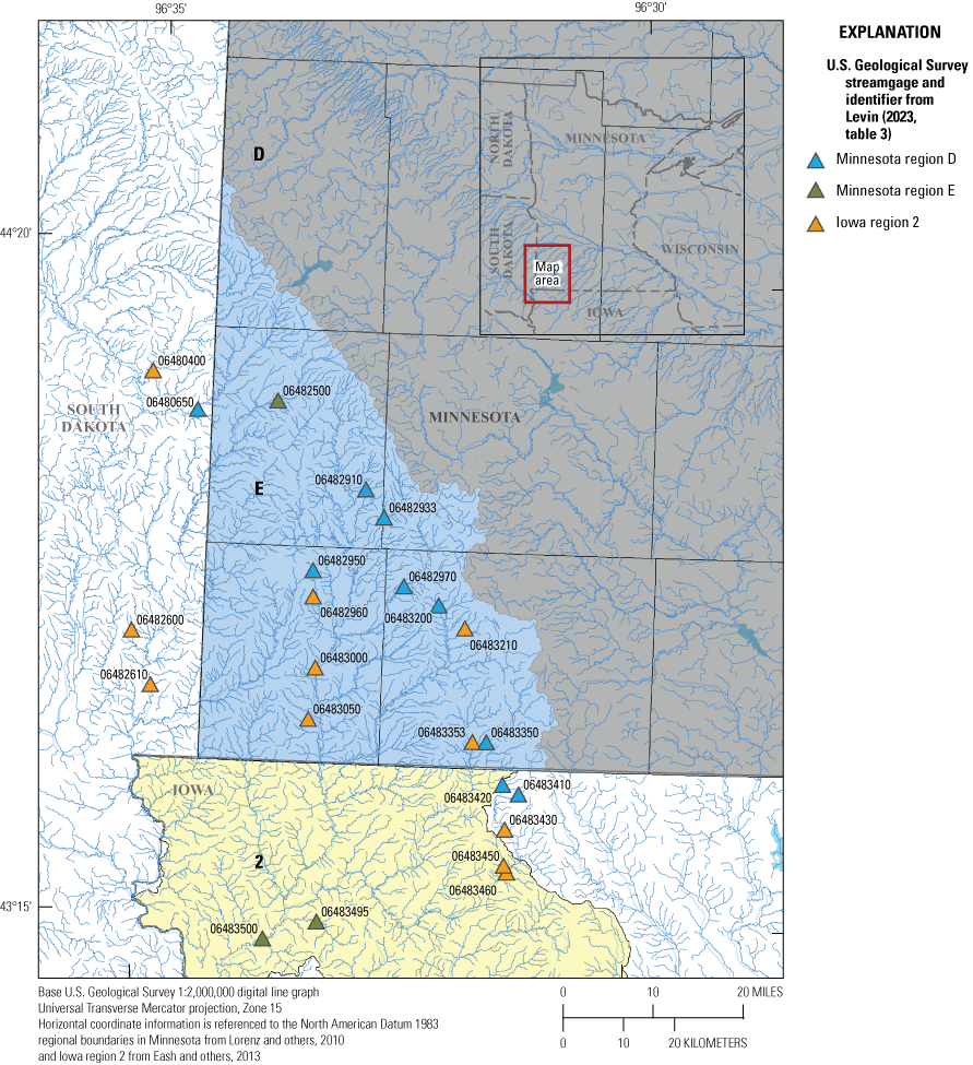
Most streamgages shown are in regions D and E. — Figure 2.
Equations (region E, region D, or Iowa region 2) that produce the lowest relative error in estimating the 0.01 annual exceedance probability for streamgages used to produce equations in region E (Levin, 2023, table 3).

The performance metrics reported in Levin (2023, table 3) are measures of average model uncertainty based on all streamgages used in the model, but they are not representative of the uncertainty for a single estimated AEPD. Practitioners may be interested in the uncertainty associated with the estimate of a specific flow value at a specific location. One such measure of site-specific uncertainty is a prediction interval. A prediction interval is a range of values that will encompass the true value with some nominal probability. For example, a 90-percent prediction interval for an estimated AEPD indicates there is a 90-percent probability that the true value of the AEPD is within the interval range. Whereas prediction intervals for OLS regressions can be easily computed from the standard error of the regression equation, prediction intervals for GLS regressions that are used in this report must account for the cross-correlations between peak-flow time series at all streamgages and the differing lengths of peak-flow record. Tasker and Driver (1988) developed a method for estimating the prediction interval of a GLS estimate:

\frac{Q}{C} < Q < Q C

,

(1)

where

Q: is the estimated AEPD at an ungaged site predicted from the regression equation, and
C: is computed as:

C = 10^{t_{(\frac{α}{2}, n - p)} S E_{p, i}}

,

(2)

where

$t_{(\frac{a}{2}, n - p)}$: is the critical value from a student’s t-distribution for an α-level, and degrees of freedom (n–p). Critical values for 90-percent (α=0.1) prediction intervals for each equation are listed in Levin (2023, tables 4a–4f), and
SE_p,i: is the critical value from a student’s t-distribution for an α-level, and degrees of freedom (n–p). Critical values for 90-percent (α=0.1) prediction intervals for each equation are listed in Levin (2023, tables 4a–4f).

The standard error of prediction for ungaged site i is computed as

S E_{(p, i)} = {[M E V + X_{i} U X_{i}^{T}]}^{0.5}

,

(3)

where

MEV: is the model error variance,
X_i: is a row vector of basin characteristics for ungaged site i and starting with a 1 as a placeholder for the intercept term,
U: is the covariance matrix for the regression coefficients, and
$X_{i}^{T}$: is the matrix transpose of X_i.

Note that although the terminology is similar, the standard error of prediction for a site (SE_p_,_i) is different than the standard error of prediction for the regression equation (S_p). Values for

t_{(\frac{a}{2}, n - p)}

, MEV, and U for each regression table are listed in Levin (2023, tables 4a–4f). The example below demonstrates the procedure for computing the 90-percent prediction interval at a specific location.

Example 1

This example demonstrates the procedure to compute a 90-percent confidence interval for the 0.01 AEP at an ungaged site. For illustration purposes, basin characteristics from streamgage 05355100, Little Cannon River tributary (fig. 1, map number 212), in region F were used (Levin, 2023, table 1f). This site has a drainage area of 2.22 square miles, and precipitation minus potential evaporation (PMPE) of 133.26 millimeters. Basin characteristics for ungaged locations in Minnesota can be obtained using the StreamStats web application (https://streamstats.usgs.gov/ss/; Ries and others, 2017). Below are the steps to follow:

First, the estimate of the Q_1% flood for this site is obtained using the GLS regression equation in Levin (2023, table 2f):

log₁₀ Q_1% = 2.446 + 0.519 × log₁₀ (DRNAREA) + 0.003 × PMPE ;

log₁₀ Q_1% = 2.446 + 0.519 × log₁₀ (2.216) + 0.003 × 133.265 =3.025;

Q_1% =10^3.025 = 1,059.254 ft³/s
Compute the vector (X_i) of log-transformed basin characteristics:

X_i= {1, log₁₀(2.216), 133.265)};

X_i={1, 0.346,0, 133.265)
Find the covariance matrix for the regression coefficients (U) for the AEP 0.01 (Q1%) regression equation from Levin (2023, table 4f).
To compute the $X_{i} U X_{i}^{T}$ term in equation 3, first perform matrix multiplication of X_i and U to get X_iU and then multiply X_iU and $X_{i}^{T}$ :

X_iU= X_i _× U = {0.0157765, −0.0016085, −0.0000655} ;

$X_{i} U X_{i}^{T}$ _i = X_iU × $X_{i}^{T}$ = 0.0064798
Obtain the model error variance (MEV) for the AEP 0.01 (Q1%) regression equation from Levin (2023, table 4f) and compute SE_p_,_I using equation 3:

$S E_{p, I} = {[M E V + X_{i} U X_{i}^{T}]}^{0.5} = {(0.023 + 0.0064798)}^{0.5} = 0.1726$
Compute C using equation 2. The critical value can be obtained for each region from Levin (2023, tables 2a–2f). In the case of the 0.01 AEP for a streamgage in region F, the critical value is 1.6811 (Levin, 2023, table 2f), so that:

$C = 10^{t (\frac{a}{2}, n - p) S E_{p, i}} = 10^{(1.6811 * 0.1726)} = 1.95055$ .
The 90-percent prediction interval is computed from equation 1 as:

(1,059.254 / 1.95055) < Q < (1,059.254 × 1.95055, or

543.1 ft³/s < Q < 2,066.1 ft³/s

Web Application for Solving Regional Regression Equations

The Minnesota StreamStats web application (https://streamstats.usgs.gov/ss/; Ries and others, 2017) plans to update the peak-flow frequency regression equations from this report to provide peak-flow frequency estimates for unregulated sites in Minnesota. The web application includes (1) a mapping tool to specify a location on a stream where peak-flow statistics are desired, and (2) an automated GIS procedure that measures the required basin characteristics and solves the regression equations to estimate peak-flow statistics for user-selected sites.

Application of Regional Regression Equations

The regression equations developed in this study can be used to generate peak-flow frequency estimates for sites on ungaged or gaged streams. Peak-flow frequency estimates for streamgages may be improved by computing a weighted-average value of two independent estimates: the at-site log-Pearson Type III frequency curve estimate and the appropriate regression equation estimate. By weighting each estimate with an appropriate weighting factor, the resulting weighted-average value will represent an improved estimate (Interagency Advisory Committee on Water Data, 1982). This section describes the procedures for estimating flood magnitudes (1) at a streamgage, (2) an ungaged stream, and (3) an ungaged location on a gaged stream.

Estimating the Weighted Peak-Flow Frequency for a Streamgage

Two estimates of peak-flow frequency for a streamgage are available: one from the at-site log-Pearson Type III frequency curve and the other from the appropriate peak-flow frequency regression equation developed in this study. A theoretically improved estimate of peak-flow frequency for a streamgage can be calculated if the individual estimates are independent and the variances of the individual estimates can be determined. If the independent estimates are weighted inversely proportional to their respective variances, then the variance of the weighted-average estimate will be less than the variances associated with each individual estimate (Tasker, 1975; Interagency Advisory Committee on Water Data, 1982).

For a particular exceedance probability, the variance of prediction from the log-Pearson Type III analysis at a streamgage (V_P₍_g₎_s) is estimated from the expected moments algorithm, as described in Bulletin 17C (England and others, 2019). The magnitude of the variance associated with the at-site frequency-curve estimate is dependent on the length of record; the mean, standard deviation, and skew of the fitted log-Pearson Type III frequency curve; and the accuracy of the method used to determine the generalized skew (Gotvald and others, 2009). The V_site_,_LP₃ for all streamgages in this study, which were computed using the PeakFQ, version 7.3 (Flynn and others, 2006; Veilleux and others, 2014), are presented in Levin (2023, tables 5a–5f).

The variance of prediction for a streamgage derived from the regional regression equation (V_P₍_g₎_r) is computed during the regression fitting process and is dependent on the error covariance matrix, and site-specific basin characteristics (Eng and others, 2009). Variance of prediction derived from the regional regression equations were computed using the WREG package in R (Farmer, 2017; Levin, 2023, tables 5a–5f).

Using the variances from the two independent peak-flow frequency estimates, the weighted-average peak-flow frequency estimate is computed using the following equation (Gotvald and others, 2009):

l o g_{10} Q_{P (g) w} = \frac{V_{P (g) r} x l o g_{10} Q_{P (g) s} + V_{P (g) r} x 10 Q_{P (g) r}}{V_{P (g) r} + V_{P (g) s}}

,

(4)

where

Q_P(g)w: is the weighted peak-flow estimate for a P-percent annual exceedance probability at a streamgage, g, in cubic feet per second;
Q_P(g)s: is the peak-flow estimate for a P-percent annual exceedance probability at a streamgage, g, computed from the station log-Pearson Type III analysis from Levin (2023, tables 1a–1f), in cubic feet per second;
Q_P(g)r: is the peak-flow estimate for the P-percent annual exceedance probability at a streamgage, g, computed from the appropriate regression equation in Levin (2023, tables 2a–2f), in cubic feet per second;
V_P(g)s: is the variance of prediction of a peak-flow estimate for the P-percent annual exceedance probability at a streamgage, g, from station log-Pearson Type III analysis in Levin (2023, table 5a–5f) in logarithm units; and
V_P(g)r: is the variance of prediction of a peak-flow estimate for the P-percent annual exceedance probability at a streamgage, g, associated with the appropriate regression equation in Levin (2023, tables 5a–5f), in logarithm units.

The variance of prediction for a weighted peak flow estimate is computed using the following equation:

V_{P (g) w} = \frac{V_{P (g) s} x V_{P (g) r}}{V_{P (g) s} + V_{P (g) r}}

(5)

Confidence intervals for a weighted estimate are determined using a weighted variance of prediction, computed using the following equation:

C I_{95 %} = [10^{(l o g Q_{P (g) w} - 1.96 \sqrt{V_{P (g) w}})}, 10^{(l o g Q_{P (g) w} + 1.96 \sqrt{V_{P (g) w}})}]

,

(6)

where

CI_P₍_g_)95%: is the 95-percent confidence interval of a weighted peak flow estimate for a P-percent annual exceedance probability at a streamgage, g, in cubic feet per second.

Estimating the Peak-Flow Frequency for an Ungaged Site

The procedure for estimating peak-flow frequency for selected exceedance probabilities for a specific ungaged site depends on whether the site is near a streamgage on the same stream or is on an ungaged stream. For an ungaged site near a streamgage on the same stream, the drainage-area ratio method for estimating the frequency may be used. The drainage-area ratio method assumes that the streamflow for a site of interest can be estimated by multiplying the ratio of the drainage area for the site of interest and the drainage area for a nearby streamgage by the log-Pearson Type III peak flow estimate for the nearby streamgage. Generally, this method should be used when the drainage area for an ungaged site is within 50 percent of the drainage area for the nearby streamgage (Ries and Dillow, 2006). For an ungaged site on an ungaged stream, the regional regression equations developed for this study should be used to estimate peak-flow frequencies.

Regression-Weighted and Area-Weighted Estimates for an Ungaged Site on a Gaged Stream

For an ungaged site on a stream with a streamgage that has 10 or more years of peak-flow record, the peak-flow frequency estimate from the appropriate regression equation for the ungaged site can be combined with the weighted-average peak-flow frequency estimate, Q_P(g)w, from equation 4, and the regression equation peak-flow frequency estimate from the nearby streamgage to produce an improved estimate. Sauer (1974) and Verdi and Dixon (2011) presented the following regression-weighted equation to improve the peak-flow frequency estimate for an ungaged site on a stream with a streamgage:

Q_{P (u) w} = (\frac{2 |A_{g} - A_{u}|}{A_{g}}) + (1 - \frac{2 |A_{g} - A_{u}|}{A_{g}}) (\frac{Q_{P (g) w}}{Q_{P (g) r}}) Q_{) (u) r}

,

(7)

where

Q_P(u)w: is the regression-weighted estimate of peak flow for the P-percent annual exceedance probability at an ungaged site, u, in cubic feet per second;
Q_P(g)w: is the weighted-average peak-flow estimate for the P-percent exceedance probability at streamgage, g, (from eq. 4), in cubic feet per second;
Q_P(g)r: is the peak-flow estimate for the P-percent exceedance probability at a streamgage from the appropriate regression equation, in cubic feet per second;
Q_P(u)r: is the peak-flow estimate for the P-percent exceedance probability at an ungaged site, from the appropriate regression equation, in cubic feet per second;
A_g: is the drainage area associated with a streamgage, in square miles; and
A_u: is the drainage area associated with an ungaged site, in square miles.

If the drainage area associated with the ungaged site is between 50 and 150 percent of the drainage area associated with the streamgage, equation 7 is applicable. If the drainage area associated with the ungaged site is less than 50 percent or greater than 150 percent of the area associated with the streamgage, then no weighting adjustment is applied to the peak-flow frequency regression estimate for the ungaged site.

Additional Considerations in Applying Peak-Flow Estimation Techniques

The accuracy of the regression equation is limited by the uncertainty of the input data. Uncertainty has two components: (1) variance, a measure of the random variation about the true value; and (2) bias, the consistent deviation of the value from the true value. How well the peak-flow estimates from the log-Pearson Type III analysis of the recorded annual peak flows predicts the actual population of peak flows depends on the sample size, the accuracy of each recorded peak value, and how well the log-Pearson Type III distribution fits the actual distribution (Interagency Advisory Committee on Water Data, 1982).

The accuracy of the regression estimate also is affected by errors in the explanatory variables. Errors in quantifying the basin characteristics result from an inability to completely describe the effect of those characteristics. For example, the effects of lakes depend on their size and location in the basin and in the stream channels, but the explanatory variable LAKEAREA is simply expressed as a percentage of total drainage area without regard to size or location.

Errors in peak flow estimates from a log-Pearson Type III analysis may occur when the period of record is short (less than 20 years) or when annual peak flows from a long-discontinued gage do not reflect current conditions. Bias of a peak-flow estimate can result if peak-flow data were collected only during a short period in the past that does not reflect the long-term population of peak flows. Long-term trends in annual peak streamflow owing to climate or anthropogenic changes can result in bias in the resulting flood estimate. Flood-frequency analysis in the presence of a long-term trend in annual peak streamflows is an active field of research. Trends in annual peak streamflows were not addressed in this study, but regional trend studies are currently underway for Minnesota and nearby States.

The accuracy of an estimate made using the techniques presented in this report also can be affected by the user. Each user will make certain decisions based on their best judgment about the actual outline of the drainage basin, the path of the main channel, interpolation of generalized runoff, and the source of lake and wetland data. These individual sources of error can be reduced by use of shared computer datasets that are updated as improved information becomes available and by the use of a GIS that provides consistent results.

The accuracy of peak-flow estimates made at sites immediately downstream from a lake or ponded area, where the storage capacity could substantially alter peak-flow characteristics, can be improved by a routing adjustment. In such places, the frequency relations could be used as an aid in developing a hydrograph of the inflow and then a simulation of that flow can be routed through the lake to determine the peak of the outflow. The values of the explanatory variables used in this analysis were all computed from consistent datasets using a GIS. Careful analysis using the best-available topographic maps should provide accurate estimates of drainage area, main-channel slope, percentage lake area in a watershed, and percent storage (percentage watershed area covered by lakes and wetlands). Regression equations are not valid in basins that are outside of the range of drainage areas and percent lakes used in the dataset (Levin, 2023, tables 1a–1f). Regression estimates extrapolated outside these conditions have greater uncertainty. The National Streamflow Statistics program (USGS, 2007) will issue a warning message if the estimated peak flow is an extrapolation beyond the data on which the estimate is based.

Summary

Regression analysis methods were used to develop and update equations that can be used to estimate the magnitude and frequency of peak flows on streams in Minnesota (excluding the Lake of the Woods, Rainy River Basin) and adjacent areas in the neighboring States of Iowa and South Dakota. Hydraulic engineers use peak streamflow data to inform the designs of bridges, culverts, and dams; and water managers use peak streamflow data to inform regulation and planning activities.

Estimates of peak-flow magnitudes for 66.7-, 50-, 20-, 10-, 4-, 2-, 1-, and 0.2-percent annual exceedance probabilities equivalent to annual flood-frequency recurrence intervals of 1.5-, 2-, 5-, 10-, 25-, 50-, 100-, and 500-year recurrence intervals, respectively, are presented for 298 streamgages on the basis of data collected through September 30, 2019.

Geographic information system software was used to calculate values for basin characteristics that were determined to be potential explanatory variables in the regression analyses. Regression equations were developed for six of the seven hydrologic regions in Minnesota to calculate peak-flow frequency statistics for ungaged locations within the respective regions. Peak-flow frequency information was subsequently used in regression analyses to develop equations relating peak flows for selected recurrence intervals to various physical and climatic characteristics. The statistically derived techniques can be used to estimate peak flow on ungaged streams smaller than 1,870 square miles in the study area.

The final regression equations were selected based on minimizing values of the standard model error and the standard error of prediction while maximizing values of the pseudo coefficient of determination, followed by examination of regression residuals. Updated peak-flow frequency data, peak-flow regional regression frequency data, and weighted peak-flow frequency data for streamgages used in the study are provided. The application of regional regression equations for determining weighted peak-flow frequency data for streamgages and at ungaged sites is described. The procedure for estimating peak-flow frequency for selected exceedance probabilities for a specific ungaged site depends on whether the site is near a streamgage on the same stream or is on an ungaged stream. For an ungaged site near a streamgage on the same stream, a drainage-area ratio method can be applied. For an ungaged site on an ungaged stream, the regional regression equations developed for this study should be used.

Equations developed in this study apply only to stream sites where flows are not substantially affected by regulation, diversion, or urbanization. All equations presented in this study will be incorporated into StreamStats, a web-based geographic information system tool developed by U.S. Geological Survey. StreamStats allows users to obtain streamflow statistics, basin characteristics, and other information for user-selected locations on streams through an interactive map.

Acknowledgments

The authors want to thank Ryan Thompson, Amanda Whaling, and Padraic Oshea, U.S. Geological Survey, for assisting with analyses and review.

References Cited

Arneson, L.A., Zevenbergen, L.W., Lagasse, P.F., and Clopper, P.E., 2012, Evaluating scour at bridges (5th ed.): Federal Highway Administration, Publication No. FHWA–HIF–12–003, Hydraulic Engineering Circular No. 18, 340 p., accessed March 15, 2013, at https://www.fhwa.dot.gov/engineering/hydraulics/pubs/hif12003.pdf.

Buto, S.G., and Anderson, R.D., 2020, NHDPlus High Resolution (NHDPlus HR)—A hydrography framework for the Nation: U.S. Geological Survey Fact Sheet 2020–3033, 2 p., accessed on February 2021 at https://doi.org/10.3133/fs20203033.

Center for Research in Water Resources, 2003, Arc Hydro Online Support System: accessed August 2008 at http://www.crwr.utexas.edu/giswr/hydro/ArcHOSS/index.Cfm.

Cohn, T.A., England, J.F., Berenbrock, C.E., Mason, R.R., Stedinger, J.R., and Lamontagne, J.R., 2013, A generalized Grubbs-Beck test statistic for detecting multiple potentially influential low outliers in flood series: Water Resources Research, v. 49, no. 8, p. 5047–5058, accessed on June 2018 at https://doi.org/10.1002/wrcr.20392.

Eash, D.A., Barnes, K.K., and Veilleux, A.G., 2013, Methods for estimating annual exceedance-probability discharges for streams in Iowa, based on data through water year 2010: U.S. Geological Survey Scientific Investigations Report 2013–5086, 63 p. with appendix. [Also available at https://doi.org/10.3133/sir20135086.]

Eng, K., Chen, Y.-Y., and Kiang, J.E., 2009, User’s guide to the weighted-multiple-linear-regression program (WREG ver. 1.0): U.S. Geological Survey Techniques and Methods, book 4, chap. A8, 21 p., accessed September 2015 at https://doi.org/10.3133/tm4A8.

England, J.F., Jr., Cohn, T.A., Faber, B.A., Stedinger, J.R., Thomas, W.O., Jr., Veilleux, A.G., Kiang, J.E., and Mason, R.R., Jr., 2019, Guidelines for determining flood flow frequency—Bulletin 17C: U.S. Geological Survey Techniques and Methods, book 4, chap. B5, 148 p. [Also available at https://doi.org/10.3133/tm4B5.]

Farmer, W., 2017, USGS-R/WREG—USGS WREG (ver. 2.02): U.S. Geological Survey software release, accessed June 2023 at https://rdrr.io/github/USGS-R/WREG.

Federal Emergency Management Agency, 2002, National Flood Insurance Program—Program description: Federal Emergency Management Agency, 37 p. [Also available at https://www.arkansasfloods.org/wp-content/uploads/2014/06/NFIP-Program-Description.pdf.]

Fischer, E.E., 1995, Potential-scour assessments and estimates of maximum scour at selected bridges in Iowa: U.S. Geological Survey Water-Resources Investigations Report 95–4051, 75 p. [Also available at https://doi.org/10.3133/wri954051.]

Flynn, K.M., Kirby, W.H., Mason, R., and Cohn, T.A., 2006, Estimating magnitude and frequency of floods using the PeakFQ program: U.S. Geological Survey Fact Sheet 2006–3143, 2 p. [Also available at https://doi.org/10.3133/fs20063143.]

Gotvald, A.J., Feaster, T.D., and Weaver, J.C., 2009, Magnitude and frequency of rural floods in the southeastern United States, 2006—Volume 1, Georgia: U.S. Geological Survey Scientific Investigations Report 2009–5043, 120 p. [Also available at https://doi.org/10.3133/sir20095043.]

Grubbs, F.E., and Beck, G., 1972, Extension of sample sizes and percentage points for significance tests of outlying observations: Technometrics, v. 10, no. 4, p. 211–219. [Also available at https://doi.org/10.1080/00401706.1972.10488981.]

Guetzkow, L.C., 1977, Techniques for estimating magnitude and frequency of floods in Minnesota: U.S. Geological Survey Water-Resources Investigations Report 77–31, 33 p. [Also available at https://doi.org/10.3133/wri7731.]

Hartigan, J.A., and Wong, M.A., 1979, A k-means clustering algorithm: Applied Statistics, v. 28, no. 1, p. 100–108. [Also available at https://doi.org/10.2307/2346830.]

Homer, C.H., Fry, J.A., and Barnes, C.A., 2012, The National Land Cover Database: U.S. Geological Survey Fact Sheet 2012‒3020, 4 p. [accessed on August 2018 at https://doi.org/10.3133/fs20123020.]

Hu, L., Nikolopoulos, E.I., Marra, F., and Anagnostou, E.N., 2019, Sensitivity of flood frequency analysis to data record, statistical model, and parameter estimation methods: An evaluation over the contiguous United States, Journal of Flood Risk Management, v 13, no. 1, art. e12580, 13 p., accessed May 2020 at https://doi.org/10.1111/jfr3.12580.

Hydrometeorological Design Studies Center, 2020, Flood Frequency Data Server (PFDS): National Oceanic and Atmospheric Association, National Weather Service database, accessed September 2020 at https://hdsc.nws.noaa.gov/hdsc/pfds/pfds_gis.html. [Digital data downloaded were 24-hour 100-year precipitation frequency estimates for Midwestern States based on precipitation data collected between 1836 and 2013.]

Interagency Advisory Committee on Water Data, 1982, Guidelines for determining flood-flow frequency: Reston, Va., U.S. Geological Survey, Bulletin 17B of the Hydrology Subcommittee, Office of Water Data Coordination, 183 p. [Also available at https://water.usgs.gov/osw/bulletin17b/bulletin_17B.html.]

Jacques, J.E., and Lorenz, D.L., 1987, Techniques for estimating the magnitude and frequency of floods in Minnesota: U.S. Geological Survey Water-Resources Investigations Report 87–4170, 48 p. [Also available at https://doi.org/10.3133/wri874170.]

Kessler, E.W., Lorenz, D.L., and Sanocki, C.A., 2013, Methods and results of peak-flow frequency analyses for streamgages in and bordering Minnesota, through water year 2011: U.S. Geological Survey Scientific Investigations Report 2013–5110, 43 p. [Also available at https://doi.org/10.3133/sir20135110.]

Levin, S.B., 2021, PeakFQ input and output files for 298 streamgages in Minnesota, Iowa, and South Dakota through water year 2019, U.S. Geological Survey, https://doi.org/10.5066/P9UNQ0IV.

Levin, S.B., 2023, Model archive of regional flood frequency equations for Minnesota streams: U.S. Geological Survey data release, https://doi.org/10.5066/P9T1HO7Q.

Lorenz, D.L., 1997, Generalized skew coefficients for flood-frequency analysis in Minnesota: U.S. Geological Survey Water-Resources Investigations Report 97–4089, 15 p. [Also available at https://doi.org/10.3133/wri974089.]

Lorenz, D.L., Carlson, G.H., and Sanocki, C.A., 1997, Techniques for estimating peak flow on small streams in Minnesota: U.S. Geological Survey Water-Resources Investigations Report 97–4249, 42 p. [Also available at https://doi.org/10.3133/wri974249.]

Lorenz, D.L., Sanocki, C.A., and Kocian, M.J., 2010, Techniques for estimating the magnitude and frequency of peak flows on small streams in Minnesota based on data through water year 2005: U.S. Geological Survey Scientific Investigations Report 2009–5250, 54 p. [Also available at https://doi.org/10.3133/sir20095250.]

Lorenz, D.L., and Ziegeweid, J.R., 2016, Methods to estimate historical daily streamflow for ungaged stream locations in Minnesota: U.S. Geological Survey Scientific Investigations Report 2015–5181, 18 p. [Also available at https://doi.org/10.3133/sir20155181.]

Minnesota Department of Natural Resources, 2009, Data deli: accessed February 2009 https://gisdata.mn.gov/content/?q=node/70.

Patterson, J.L., and Gamble, G.R., 1968, Magnitude and frequency of floods in the United States, Part 5: Hudson Bay and Upper Mississippi River Basins, U.S. Geological Survey Water-Supply Paper 1678, 546 p. [Also Available at https://doi.org/10.3133/wsp1678.]

Prior, C.H., 1949, Magnitude and frequency of floods in Minnesota: St. Paul, Minnesota Department of Conservation, Division of Waters Bulletin 1, 128 p.

Prior, C.H., and Hess, J.H., 1961, Floods in Minnesota—Magnitude and frequency: St. Paul, Minnesota Department of Conservation, Division of Waters Bulletin 12, 142 p.

R Core Team, 2020, R—A language and environment for statistical computing: Vienna, Austria, R Foundation for Statistical Computing software, accessed September 2021 at https://www.r-project.org/index.html.

Ries, K.G., III, and Dillow, J.J.A., 2006, Magnitude and frequency of floods on nontidal streams in Delaware: U.S. Geological Survey Scientific Investigations Report 2006–5146, 59 p. [Also available at https://doi.org/10.3133/sir20065146.]

Ries, K.G., III, Newson J.K., Smith, M.J., Guthrie, J.D., Steeves, P.A., Haluska, T.L., Kolb, K.R., Thompson, R.F., Santoro, R.D., and Vraga, H.W., 2017, StreamStats, version 4: U.S. Geological Survey Fact Sheet 2017–3046, 4 p. [Also available at https://doi.org/10.3133/fs20173046.] [Supersedes USGS Fact Sheet 2008–3067.]

Sando, S.K., Driscoll, D.G., and Parrett, C., 2008, Peak-flow frequency estimates based on data through water year 2001 for selected streamflow-gaging stations in South Dakota: U.S. Geological Survey Scientific Investigations Report 2008–5104, 367 p. [Also available at https://doi.org/10.3133/sir20085104.]

Sanocki, C.A., Williams-Sether, T., Steeves, P.A., and Christensen, V.G., 2019, Techniques for estimating the magnitude and frequency of peak flows on small streams in the binational U.S. and Canadian Lake of the Woods–Rainy River Basin upstream from Kenora, Ontario, Canada, based on data through water year 2013: U.S. Geological Survey Scientific Investigations Report 2019–5012, 17 p. [Also available at https://doi.org/10.3133/sir20195012.]

Sauer, V.B., 1974, Flood characteristics of Oklahoma streams—Techniques for calculating magnitude and frequency of floods in Oklahoma, with compilations of flood data through 1971: U.S. Geological Survey Water-Resources Investigation Report 73–52, 46 p. [Also available at https://doi.org/10.3133/wri7352.]

Soil Survey Staff, 2012, Soil Survey Geographic Database (SSURGO): Natural Resources Conservation Service database, accessed April 3, 2013, at http://www.nrcs.us da.gov/wps/portal/nrcs/main/soils/survey/.

Solstad, J., and Vaughn, S., 2007, The Minnesota Lake Watershed Delineation (Lakeshed) Project: Minnesota Department of Natural Resources, accessed August 2007 at https://www.dnr.state.mn.us/watersheds/lakeshed_project.html.

Stedinger, J.R., and Tasker, G.D., 1985, Regional hydrologic analysis 1—Ordinary, weighted, and generalized least squares compared: Water Resources Research, v. 21, no. 9, p. 1421–1432. [Also available at https://doi.org/10.1029/WR021i009p01421.]

Tasker, G.D., 1975, Combining estimates of low-flow characteristics of streams in Massachusetts and Rhode Island: Journal of Research of the U.S. Geological Survey, v. 3, no. 1, p. 107–112.

Tasker, G.D, and Driver, N.E., 1988, Nationwide regression models for predicting urban runoff water quality at unmonitored sites: Water Resources Bulletin, v. 24, no.5, p. 1091-1101. [Also available at https://doi.org/10.1111/j.1752-1688.1988.tb03026.x.]

Tasker, G.D., and Stedinger, J.R., 1989, An operational GLS model for hydrologic regression: Journal of Hydrology (Amsterdam), v. 111, nos. 1–4, p. 361–375. [Also available at https://doi.org/10.1016/0022-1694(89)90268-0.]

U.S. Geological Survey [USGS], 2007, National streamflow statistics program—Estimating high and low streamflow statistics for ungaged sites: U.S. Geological Survey Fact Sheet 2007–3010, 2 p., accessed June 2015 at https://doi.org/10.3133/fs20073010.

U.S. Geological Survey [USGS], 2013, National Elevation Dataset, 1/3 arc second: U.S. Geological Survey digital data, accessed January 2013 at https://viewer.nationalmap.gov/.

U.S. Geological Survey [USGS], 2019, USGS water data for the Nation: U.S. Geological Survey National Water Information System database, accessed July 2019 at https://doi.org/10.5066/F7P55KJN.

U.S. Fish and Wildlife Service, 2008, National Wetlands Inventory: Washington, D.C., U.S. Fish and Wildlife Service database, accessed November 2008 at https://www.fws.gov/wetlands/Data/Data-Download.html.

Veilleux, A.G., Cohn, T.A., Flynn, K.M., Mason, R.R., Jr., and Hummel, P.R., 2014, Estimating magnitude and frequency of floods using the PeakFQ 7.0 program: U.S. Geological Survey Fact Sheet 2013–3108, 2 p., accessed January 2015 at https://doi.org/10.3133/fs20133108.

Verdi, R.J., and Dixon, J.F., 2011, Magnitude and frequency of floods for rural streams in Florida, 2006: U.S. Geological Survey Scientific Investigations Report 2011–5034, 69 p., 1 pl. [Also available at https://doi.org/10.3133/sir20115034.]

Walker, J.F., and Krug, W.R., 2003, Flood-frequency characteristics of Wisconsin streams: U.S. Geological Survey Water-Resources Investigations Report 2003–4250, 16 p. [Also available at https://doi.org/10.3133/wri034250.]

Wiitala, S.W., 1965, Magnitude and frequency of floods in the United States, Part 4: U.S. Geological Survey Water-Supply Paper 1677, 357 p. [Also available at https://doi.org/10.3133/wsp1677.]

Williams-Sether, T., 2015, Regional regression equations to estimate peak-flow frequency at sites in North Dakota using data through 2009: U.S. Geological Survey Scientific Investigations Report 2015–5096, 12 p. [Also available at https://doi.org/10.3133/sir20155096.]

Winter, T.C., 2001, The concept of hydrologic landscapes: Journal of the American Water Resources Association, v. 37, no. 2, p. 335–349, accessed January 2017 at https://doi.org/10.1111/j.1752-1688.2001.tb00973.x.

Wolock, D.M., Winter, T.C., and McMahon, G., 2004, Delineation and evaluation of hydrologic-landscape regions in the United States using geographic information system tools and multivariate statistical analyses: Environmental Management, v. 34, no. S1, suppl. 1, p. S71–S88, accessed January 2017 at https://doi.org/10.1007/s00267-003-5077-9.

Ziegeweid, J.R., Lorenz, D.L., Sanocki, C.A., and Czuba, C.R., 2015, Methods for estimating flow-duration curve and low-flow frequency statistics for ungaged locations on small streams in Minnesota: U.S. Geological Survey Scientific Investigations Report 2015–5170, 23 p. [Also available at https://doi.org/10.3133/sir20155170.]

Conversion Factors

U.S. customary units to International System of Units


Multiply	By	To obtain
Length
mile (mi)	1.609	kilometer (km)
yard (yd)	0.9144	meter (m)
Area
square mile (mi²)	259.0	hectare (ha)
square mile (mi²)	2.590	square kilometer (km²)
Flow rate
cubic foot per second (ft³/s)	0.02832	cubic meter per second (m³/s)
Hydraulic gradient
foot per mile (ft/mi)	0.1894	meter per kilometer (m/km)

Datum

Vertical coordinate information is referenced to the North American Vertical Datum of 1988 (NAVD 88).

Horizontal coordinate information is referenced to the North American Datum of 1983 (NAD 83).

Supplemental Information

A water year is the 12-month period from October 1 through September 30 and is designated by the year in which it ends.

Abbreviations

AEP: annual exceedance probability
AEPD: annual exceedance probability discharge
AVP: average variance of prediction
B17B: Bulletin 17B of the U.S. Geological Survey Hydrology Subcommittee, Office of Water Data Coordination
DEM: digital elevation model
EMA: expected moments algorithm
GIS: geographic information system
GLS: generalized least squares
MGB: Multiple Grubbs Beck
OLS: ordinary least squares
PILF: potentially influential low flow
R²: coefficient of determination
SME: standard model error
S_p: standard error of prediction
USGS: U.S. Geological Survey

For more information about this publication, contact:

Director, USGS Upper Midwest Water Science Center

1 Gifford Pinchot Drive

Madison, WI 53726

For additional information, visit: https://www.usgs.gov/centers/upper-midwest-water-science-center

Publishing support provided by the Rolla Publishing Service Center

Suggested Citation

Sanocki, C.A., and Levin, S.B., 2023, Techniques for estimating the magnitude and frequency of peak flows on small streams in Minnesota, excluding the Rainy River Basin, based on data through water year 2019: U.S. Geological Survey Scientific Investigations Report 2023–5079, 15 p., https://doi.org/10.3133/sir20235079.

ISSN: 2328-0328 (online)

Study Area

Additional publication details
Publication type	Report
Publication Subtype	USGS Numbered Series
Title	Techniques for estimating the magnitude and frequency of peak flows on small streams in Minnesota, excluding the Rainy River Basin, based on data through water year 2019
Series title	Scientific Investigations Report
Series number	2023-5079
DOI	10.3133/sir20235079
Year Published	2023
Language	English
Publisher	U.S. Geological Survey
Publisher location	Reston, VA
Contributing office(s)	Upper Midwest Water Science Center
Description	Report: v, 15 p.; Data Release; Dataset
Country	United States
State	Minnesota
Online Only (Y/N)	Y
Google Analytic Metrics	Metrics page

Techniques for Estimating the Magnitude and Frequency of Peak Flows on Small Streams in Minnesota, Excluding the Rainy River Basin, Based on Data Through Water Year 2019

Table of Contents

Links

Abstract

Introduction

Purpose and Scope

Previous Studies

Description of Study Area

Study Methods

Techniques for Estimating Peak-Flow Frequency

Peak-Flow Data

Frequency Analysis of Annual Peak-Flow Data at Selected Streamgages

Estimating Basin Characteristics

Methods Used to Define Peak-Flow Hydrologic Regions

Development of Regional Regression Equations

Accuracy and Limitations of the Regional Regression Equations

(1)

(2)

(3)

Example 1

Web Application for Solving Regional Regression Equations

Application of Regional Regression Equations

Estimating the Weighted Peak-Flow Frequency for a Streamgage

(4)

(5)

(6)

Estimating the Peak-Flow Frequency for an Ungaged Site

Regression-Weighted and Area-Weighted Estimates for an Ungaged Site on a Gaged Stream

(7)

Additional Considerations in Applying Peak-Flow Estimation Techniques

Summary

Acknowledgments

References Cited

Conversion Factors

Datum

Supplemental Information

Abbreviations

For more information about this publication, contact:

Suggested Citation

Study Area