

Machine-Learning Predictions of Groundwater Specific Conductance in the Mississippi Alluvial Plain, South-Central United States, With Evaluation of Regional Geophysical Aerial Electromagnetic Data as Explanatory Variables
Links
- Document: Report (31.1 MB pdf) , HTML , XML
- Sheet: Plate 1 (12.3 MB pdf) —Raster Predictions of Specific Conductance at Groundwater Wells by Depth in the Mississippi Alluvial Plain Region
- Dataset: USGS Dataset —USGS water data for the Nation
- Data Release: USGS Data Release - Machine-learning model predictions and rasters of groundwater salinity in the Mississippi Alluvial Plain
- NGMDB Index Page: National Geologic Map Database Index Page (html)
- Download citation as: RIS | Dublin Core
Acknowledgments
This research was supported by the U.S. Geological Survey Water Availability and Use Science Program Mississippi Alluvial Plain Regional Water Availability Study.
Abstract
The Mississippi Alluvial Plain, located in the south-central United States, is undergoing long-term groundwater-level declines within the surficial Mississippi River Valley alluvial aquifer (hereinafter referred to as “alluvial aquifer”), which has raised concerns about future groundwater availability. In some parts of the alluvial aquifer, groundwater availability for common uses such as irrigation, public supply, and domestic use is limited by quality (for example, high salinity) rather than quantity of water stored in the aquifer. The Mississippi Alluvial Plain region has an abundance of water-quality measurements in the alluvial aquifer and deeper aquifers; however, large areas lack direct measurements of salinity to evaluate regional groundwater availability. Statistical models can interpolate between wells to fill in spatial data gaps. In 2021, the U.S. Geological Survey trained two boosted regression tree (BRT) machine-learning models on specific conductance data available between 1942 and 2020 to predict spatially continuous surfaces of groundwater salinity at multiple depths for the alluvial aquifer and deeper aquifers. Well construction information, water levels, and surficial variables such as geomorphology and soils were included as explanatory variables in this baseline model. Additionally, subsurface electrical resistivity data from the first aquifer-wide aerial electromagnetic (AEM) survey for the region were incorporated to create a geophysical model. This work expands on prior BRT salinity predictions of the alluvial aquifer and extends predictions south to the Gulf of Mexico, where groundwater salinity is high. AEM survey data were not available for the southern extent of the alluvial aquifer at the time of modeling. A BRT model was trained without (baseline) and with (geophysical) AEM variables to test the ability of the models to predict salinity where explanatory data are missing and response data are sparse. Additionally, model sensitivity to AEM survey data was evaluated to better understand how AEM variables influence specific conductance predictions. Model performance was improved with the addition of geophysical data, which added three-dimensional information, thereby improving salinity predictions at depth. Groundwater specific conductance predictions can help inform other geophysical investigations in the southern extent of the study area, where high groundwater specific conductance can obfuscate changes in aquifer sediment resistivity and could limit groundwater resources for agricultural, public supply, and domestic uses.
Introduction
High groundwater salinity can have major environmental and economic impacts by limiting available groundwater resources. High salinity can have negative effects on agriculture by inhibiting crop growth and reducing crop yield, depending on the salinity threshold of the species (Maas, 1993; Hardke, 2021). Groundwater with high salinity that is pumped for irrigation and then flows into nearby streams may interfere with stream ecology (Hart and others, 1990). Additionally, high salinity impacts the amount of freshwater available for human consumption; for example, the U.S. Environmental Protection Agency has a secondary maximum contaminant level of 500 milligrams per liter (mg/L) total dissolved solids (TDS; a measure of salinity) in drinking water (U.S. Environmental Protection Agency, 2022).
Effects of high groundwater salinity are observable worldwide, and impacts are more perceptible in areas where groundwater is the main source of freshwater (Welch and Hanor, 2011; Krishan, 2019). The Mississippi Alluvial Plain (fig. 1), located in the south-central United States, is no exception. Much of the groundwater in the Mississippi Alluvial Plain region is a freshwater resource with TDS concentrations less than 1,000 parts per million (ppm) (Kingsbury and others, 2014; Stanton and others, 2017), but concentrations increase—to as great as approximately 35,000 ppm—toward the Gulf of Mexico (Grubb, 1998). Additionally, there are several major areas of known high salinity in the Mississippi Alluvial Plain region: around Iberville Parish, Louisiana (Welch and Hanor, 2011); in southeastern Arkansas (Larsen and others, 2021); and around White County, Ark. (Bryant and others, 1985), as well as in smaller, localized areas that may limit the use of groundwater for agricultural, public drinking water, and domestic uses.
The Mississippi Alluvial Plain region contains the highly productive surficial Mississippi River Valley alluvial aquifer (hereinafter referred to as “alluvial aquifer”) (Ackerman, 1996; Barlow and Clark, 2011; Clark and others, 2011; Lovelace and others, 2020). The alluvial aquifer was ranked first among principal aquifers in the United States in 2015 in estimated groundwater withdrawals for irrigation, supplying about 11,745 million gallons per day (Lovelace and others, 2020). The alluvial aquifer supports an $11.9 billion industrial-scale agricultural economy (Alhassan and others, 2019). Tertiary aquifers that underlie the alluvial aquifer supply freshwater for agricultural, public drinking water, and domestic uses (Lovelace and others, 2020). Groundwater withdrawals in the alluvial aquifer and deeper aquifers have altered flow paths and created large cones of depression and have been linked to a migrating freshwater-saltwater interface and subsidence in some areas (Grubb, 1998; Clark and Hart, 2009; Jones and others, 2016). Groundwater resources in the Mississippi Alluvial Plain region are at risk for declining availability (Stanton and others, 2017). Observed declines in groundwater levels and decreased discharge to streamflow over time have prompted investigations to quantify the available groundwater resources in the Mississippi Alluvial Plain region (Ackerman, 1996; Clark and others, 2011; Killian and others, 2019; Yasarer and others, 2020).
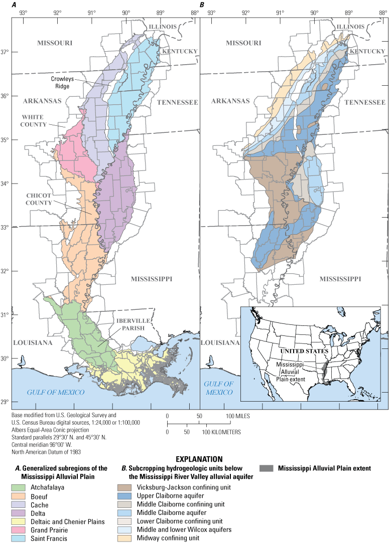
Overview of the Mississippi Alluvial Plain, south-central United States, by A, generalized subregions (Ladd and Travers, 2019) and B, subcropping hydrogeologic units (Hart and others, 2008).
Sources of salinity in the Mississippi Alluvial Plain region include but are not limited to upwelling from deeper saline aquifers, especially along regional fault lines (Kresse and Clark, 2008; Schrader, 2010; Larsen and others, 2021); subsurface dissolution of salt diapirs (Welch and Hanor, 2011); and saltwater intrusion from the Gulf of Mexico (Williamson and others, 1990; Grubb, 1998). Additionally, salinity may be concentrated at the surface as a result of evaporation where infiltration rates are low (Kresse and Clark, 2008).
Several techniques and methods have been developed to map spatial changes in groundwater quality, including geostatistical interpolation (Arslan, 2012), aerial electromagnetic (AEM) surveys of subsurface electrical conductivity (Delsman and others, 2018), and machine learning (ML) (Knierim and others, 2020). Multivariate regression analyses of hydrogeologic factors that may drive TDS concentrations were used to predict the occurrence and probability of exceedance for brackish groundwater at the national scale but were not detailed enough to delineate areas of high salinity in the Mississippi Alluvial Plain region (Stanton and others, 2017). ML predictions of groundwater salinity exist for the Mississippi embayment; however, these predictions were shown at only a single depth within the alluvial aquifer (Knierim and others, 2020). Groundwater salinity predictions at multiple depths are needed to understand how salinity changes vertically within an aquifer.
Salinity is typically quantified with TDS concentrations, but specific conductance (SC) is an easily collected measurement that describes dissolved ions. SC measures the electrical conductivity of water (Hem, 1985; Miller and others, 1988) and can correlate with concentrations of chloride and TDS, both of which have drinking water standards (U.S. Environmental Protection Agency, 2022). The Mississippi Alluvial Plain region has extensive SC data that have been collected over many decades (fig. 2) by the U.S. Geological Survey in cooperation with State agencies, including the Arkansas Natural Resources Division, the Louisiana Department of Transportation and Development, and the Mississippi Department of Environmental Quality. Although the SC dataset across the Mississippi Alluvial Plain region is large, there are still areas that do not have SC measurements, and the variation of SC with depth in the alluvial aquifer has not been characterized across the whole system.
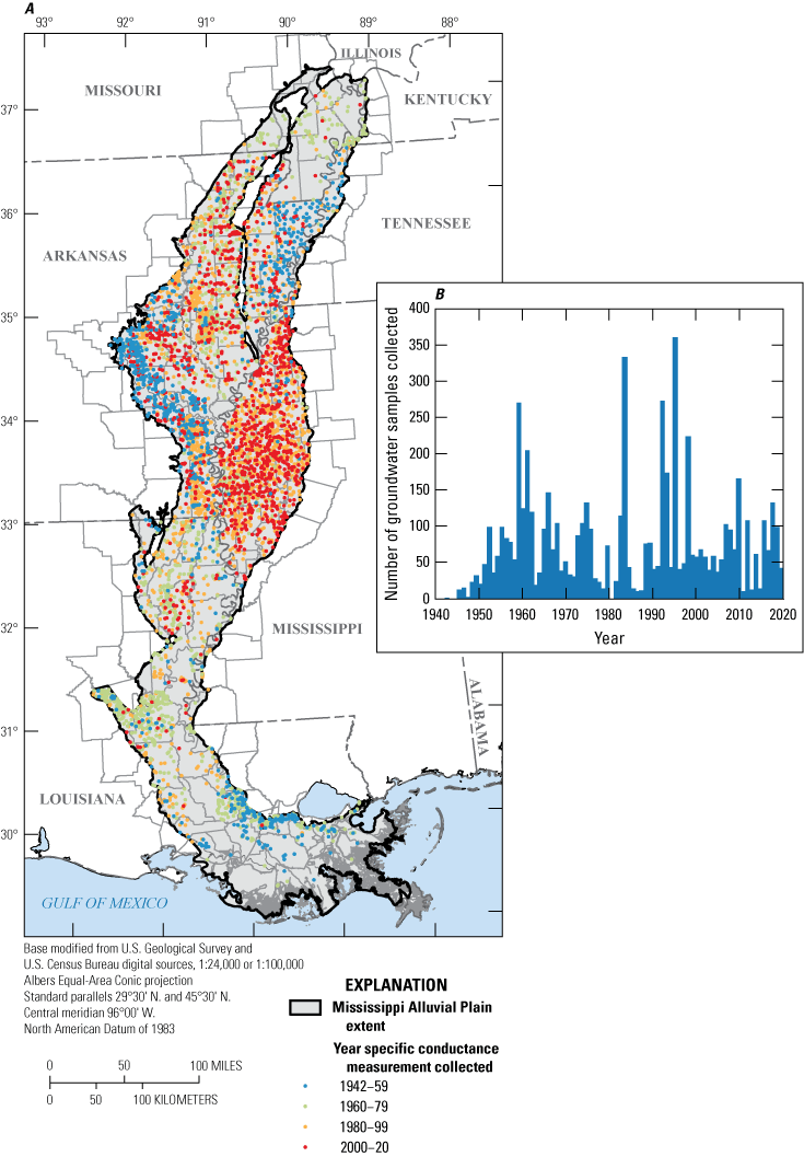
A, Spatiotemporal distribution of groundwater samples collected across the Mississippi Alluvial Plain region 1942–2020 and B, number of samples collected in each year used in the models to produce predictions of specific conductance for the region. Data from U.S. Geological Survey (2021) and Killian and Knierim (2023).
In 2021, the U.S. Geological Survey trained two boosted regression tree (BRT) ML models on SC data available between 1942 and 2020 to predict spatially continuous surfaces of groundwater salinity at multiple depths for the alluvial aquifer and deeper aquifers. This study uses ML to predict SC across the Mississippi Alluvial Plain region for the alluvial aquifer and deeper aquifers. ML can be used to predict groundwater quality across aquifers where data are unavailable by identifying patterns of explanatory variables in complex datasets (Shangguan and others, 2017; Ransom and others, 2022). A BRT model is a type of ML model that provides model stability, resistance to collinearity among predictors, and the ability to handle missing input data (Elith and others, 2008; Kuhn and Johnson, 2013). Previous studies have demonstrated that BRT models can produce accurate predictions of groundwater quality across aquifer systems (Ransom and others, 2017; Rosecrans and others, 2017; Knierim and others, 2020). This study uses BRT models to expand on efforts to model groundwater SC in the Mississippi embayment (Knierim and others, 2020), extending the predictions to the Gulf of Mexico and adding high-resolution predictions for multiple depths. Response and explanatory variables and model predictions are available in the companion U.S. Geological Survey data release (Killian and Knierim, 2023).
The objectives of this study were to (1) develop BRT models to predict SC across the Mississippi Alluvial Plain region at multiple depths for the alluvial aquifer and deeper aquifers, (2) test the ability of the models to predict where there is a paucity of groundwater SC data and explanatory variables, and (3) evaluate model performance and sensitivity to the incorporation of explanatory variables from a regional geophysical survey. Model performance was assessed by generating two BRT models, a “baseline” model that did not incorporate geophysical data and a “geophysical” model that did. The predictions will help identify where high SC could limit groundwater resources for agricultural, public drinking water, and domestic uses. The predictions will also aid in the interpretation of geophysical data by identifying where high SC may obfuscate variations in aquifer sediment resistivity.
Study Area
The Mississippi Alluvial Plain region covers parts of seven States, extending as far north as Illinois and south to the Gulf of Mexico (fig. 1). The extent of the Mississippi Alluvial Plain covers about 44,200 square miles and can be divided into seven generalized subregions to allow for subregional comparisons of data (Ladd and Travers, 2019) (fig. 1A). The subregions are bounded by major streams or other groundwater divides, such as Crowleys Ridge. For this study, the southernmost subregion, the Deltaic and Chenier Plains, was expanded to include alluvial deposits along the Mississippi River between New Orleans and Lake Pontchartrain, La., and associated water-quality data (Killian and Knierim, 2023).
The alluvial aquifer is coextensive with the Mississippi Alluvial Plain region and overlies geologic units deposited by transgressive and regressive events during the Cretaceous and Tertiary Periods (Clark and Hart, 2009). The alluvial aquifer comprises Quaternary sands, silts, and clays deposited by the ancestral Mississippi and Ohio Rivers (Renken, 1998; Arthur, 2001). The thickness of the alluvial aquifer varies across the study area and is typically between 130 and 280 feet (ft) (Hart and others, 2008). In areas where the alluvial aquifer overlies subcropping aquifer units, the bottom of the alluvial aquifer is not well defined, and different sources provide different thickness estimates (Torak and Painter, 2019a; James and Minsley, 2021). A thin layer of shallow surficial confining material of silt, clay, and fine sand is present in the alluvial aquifer but may be absent in some areas (Renken, 1998). The surficial confining material is not uniform and is thought to impede recharge to the alluvial aquifer where present (Renken, 1998). The alluvial aquifer is above a large plunging syncline that dips toward the Gulf of Mexico. There are several subcropping aquifer hydrogeologic units that are Tertiary in age that have been mapped beneath the alluvial aquifer in the Mississippi embayment part of the study area (Hart and others, 2008).
Methods
Response Variable
Response variable data included spatially distributed measurements of SC collected from domestic wells and from public-supply, irrigation, and observation wells owned by several Federal, State, and local cooperators. SC water-quality data from 6,626 wells were obtained from the U.S. Geological Survey National Water Information System (U.S. Geological Survey, 2021). The Mississippi Department of Environmental Quality provided data from an additional 888 wells with SC water-quality measurements for a total of 7,514 wells (Killian and Knierim, 2023).
Wells that were less than 400 ft below the land surface were used in the response variable dataset, reducing the number of wells available for use in the models from 7,514 to 6,042 for the final dataset (Killian and Knierim, 2023) (fig. 3). Wells that were greater than 400 ft deep were not used because the depth of investigation of AEM survey data is generally 400 ft deep across the study area (James and Minsley, 2021). Wells completed in the alluvial aquifer and deeper Tertiary aquifers were included to allow the model freedom to predict without the constraint of aquifer designation because the base of the alluvial aquifer is not well defined in some areas. The median well depth was 114 ft below land surface (Killian and Knierim, 2023). A total of 987 wells did not have a defined bottom of well screen. Most of the wells were completed in the alluvial aquifer (number of samples [n] = 5,673), 98 wells had no aquifer designation, 49 wells were completed in terrace deposits, and the remaining wells were completed in deeper aquifers (n = 222).
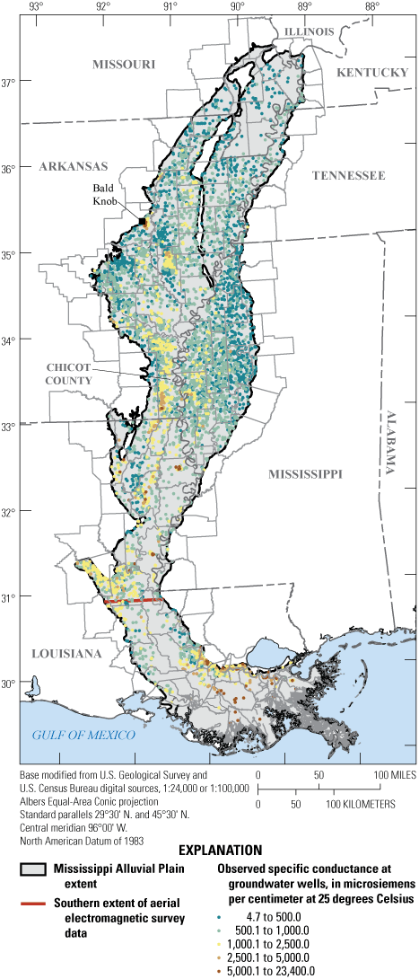
Specific conductance observed at groundwater wells screened in the Mississippi River Valley alluvial aquifer and deeper aquifers in the Mississippi Alluvial Plain region, 1942–2020 (sample size = 6,042), used to train two boosted regression tree machine-learning models. Data from U.S. Geological Survey (2021) and Killian and Knierim (2023).
Observed SC in the filtered dataset ranged from 4.7 to 23,400.0 microsiemens per centimeter at 25 degrees Celsius (µS/cm) (natural log 1.55 to 10.06) and was positively skewed (fig. 3) (Killian and Knierim, 2023). The median observation was 632 µS/cm (natural log 6.45). BRT models split the response variable data into trees that minimize variance, which will allow higher values to have a greater effect on variance. Because of how BRT models handle response variable data and because the data are positively skewed, the data were log-transformed using the natural log to reduce the relative importance of the higher values and increase the predictive accuracy for the bulk of the response variable data.
The caret package in R (Kuhn and others, 2019) was used to randomly split the response variable data into two groups: a training dataset and a holdout dataset. The training data consisted of 4,835 measurements (about 80 percent) and were used to tune the model; the remaining 1,207 measurements (about 20 percent) were held out to evaluate model performance.
Groundwater wells across the Mississippi Alluvial Plain region have varying numbers of samples ranging from one sample to continuous monitoring throughout a year or across several decades. If more than one observation existed for a well, the most recent measurement was used in model tuning and prediction. To increase the number of SC measurements for the model, samples from 1942 to 2020 were used (fig. 2). Censored values, or measurements where the value is only partially known (for example, below the detection limit of an instrument), were not included in the response variable dataset (n = 7). Some subregions of the Mississippi Alluvial Plain region—such as the Atchafalaya and the Deltaic and Chenier Plains (fig. 1A)—have not been sampled for several decades, whereas some subregions—such as the Cache and the Delta (fig. 1A)—are lacking historical measurements (fig. 2A). The number of SC measurements collected across the Mississippi Alluvial Plain region changed throughout time (fig. 2B). Because only the most recent SC measurement at each well was used in both models, information about changes in SC through time was effectively removed, and this modeling effort assumed no change in water quality over time at a well.
Explanatory Variables
Two BRT models were developed to understand the influence of geophysical explanatory variables on SC predictions: one model without geophysical variables (the “baseline” model) and one model with geophysical variables from an aquifer-wide AEM survey (the “geophysical” model). SC predictions were compared between the BRT models to quantify the change in model performance and the sensitivity of the models to geophysical variables (Knierim and others, 2020; Stackelberg and others, 2021).
Both models initially included 29 explanatory variables describing well construction information; surficial characteristics such as soils and geomorphology; positional information such as latitude, longitude, generalized subregions, and multi-order hydrologic position; depth to the water table; and year of SC measurement (table 1, at back of report). The geophysical model included the same 29 explanatory variables as the baseline model and an additional 19 geophysical variables (for a total of 48). Geophysical explanatory variables included bulk electrical resistivity (average electrical resistivity through the depth of investigation), which is sensitive to groundwater salinity and aquifer texture. Additional variables interpreted from the AEM survey included surficial confining unit top and bottom altitudes, the estimated base of the alluvial aquifer, and aquifer connectivity with streams (table 1, at back of report). More information about each explanatory variable, including name, description, dataset group, and source information, can be found in table 1 (at back of report) and Killian and Knierim (2023).
Explanatory variables were attributed to well points by using Python (Python Software Foundation, 2021) to execute a point extraction from the coincident raster cell, calculate averages for a buffer around the well, or extract a value from the depth coincident with the well screen. Point and buffer extractions were completed with the zonepy package (Clark and others, 2019). Point extraction was used to maintain high resolution of the source data, where applicable (table 1, at back of report), and for categorical explanatory variables. To account for spatial variation around a well, continuous explanatory variables were attributed using a 500-meter (m) buffer around the well. Well buffers also serve as surrogates for the contributing area (Johnson and Belitz, 2009). Two of the geophysical variables—aquifer resistivity and facies class—were attributed using the midpoint depth of the well screen and the corresponding coincident raster cell and depth slice from the AEM survey data. If well depth was unknown, resistivity and facies class were not assigned.
The year of SC measurement collection was included in the BRT models as an explanatory variable because the SC dataset spanned 78 years. Ultimately, time is inherently included in the model because of the decades over which SC measurements were collected. By explicitly including the year of measurement collection as an explanatory variable, the effect of time on SC predictions could be determined. Although the BRT models can make SC predictions for any specific year between 1942 and 2020, the models were not developed to predict SC through time. The explanatory variable dataset generally includes variables that capture conditions around 2018 (Killian and Knierim, 2023). To fully incorporate a time component in the BRT models and predict SC through time, explanatory variables that capture changes over time would also need to be included in model training.
Random noise was also included as an explanatory variable. The BRT models can determine the relative importance of each explanatory variable. Random noise was used as a benchmark to remove explanatory variables that were less influential than noise, which helped to improve model run time without impacting model performance. This method of including random noise for variable reduction is novel; however, similar approaches have been used (Ljunggren and Ishii, 2021). The random noise raster was generated with the ArcMap version 10.8 Create Random Raster tool available in the Spatial Analyst extension (Esri, 2020). The seed value was set to 2,640, and the Random Generator type was set to the default ACM599. Values in the random noise raster range from 0 to 1.
Geophysical Data Collection in the Mississippi Alluvial Plain Region and Incorporation in BRT Models
A unique aspect of the SC predictions from BRT models is incorporation of regional geophysical datasets, which provides information about the hydrogeology of the Mississippi Alluvial Plain region (Minsley and others, 2021). The geophysical data include an AEM survey, which measures resistivity signatures of water-bearing geologic materials (Smith and others, 2007). AEM survey data can help to map the thickness and extent of an aquifer. At the time of this study, the AEM survey data collected in the Mississippi Alluvial Plain region in 2019–21 covered 14,932 line-miles in the northern part of the study area and included shallow (less than about 330 ft) and deep (up to about 980 ft) estimates of inverted resistivity (mres) (James and Minsley, 2021; Minsley and others, 2021). Mres was further interpreted to estimate the bottom of the alluvial aquifer (mrvaBaseElv) and the presence or absence of surficial confining material (cnf_class). The AEM survey also included an CS-3 cesium vapor magnetometer (Scintrex Ltd., Concord, Ontario, Canada) to measure magnetic intensity (magint) and an RS-500 spectrometer radiochemical sensor (Radiation Solutions Inc., Mississauga, Ontario, Canada) to detect near-surface radioelements (predominantly potassium, uranium, and thorium) (Burton and others, 2021). These data provide three-dimensional information that has aided in the delineation of the base of the alluvial aquifer, locating where surficial confining material may be present or absent, and evaluating the degree of potential hydraulic connectivity between the alluvial aquifer and deeper subcropping aquifers (James and Minsley, 2021). At the time of this study, AEM coverage extended from the northern extent of the Mississippi Alluvial Plain region to approximately 31 degrees north latitude (figs. 3, 4), meaning that the AEM survey data did not cover the full Mississippi Alluvial Plain region. The authors sought to test how a BRT model would perform with an incomplete explanatory variable dataset.
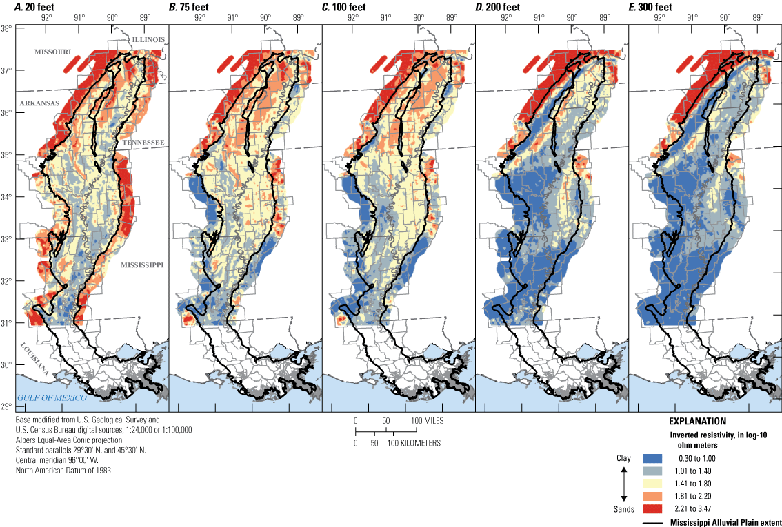
Inverted resistivity estimated from aerial electromagnetic survey data collected during 2019–21 in the Mississippi Alluvial Plain region by depth slices of A, 20 feet, B, 75 feet, C, 100 feet, D, 200 feet, and E, 300 feet (survey data from James and Minsley [2021] and Minsley and others [2021]).
Model Development
BRT models were developed in the R language (R Core Team, 2021) by leveraging the caret and gbm packages (Kuhn and others, 2019; Ridgeway, 2019). BRT is an ensemble-tree method that builds many trees with branches based on if/then statements that group data into similar homogenous groups with respect to the response variable (Kuhn and Johnson, 2013). The BRT method provides models that are more stable with better predictive performance than a single decision tree (Elith and others, 2008). The number and shape of trees in BRT models are controlled by five hyperparameters, which determine the model fit and complexity. Hyperparameters include the number of trees (nt), interaction depth (id; how deeply the trees split), shrinkage (sh; the proportion of each tree used as the model grows), minimum number of observations per node, and bagging fraction (bootstrap aggregation) (Elith and others, 2008; Kuhn and Johnson, 2013; Ridgeway, 2019).
Cross-validation (CV) tuning was used to tune the baseline and geophysical models and find the combination of hyperparameters with the best performance, or lowest root-mean-square error (RMSE) (Kuhn and others, 2019). Bagging fraction was held at the recommended value of 0.5 (Friedman, 2001) and minimum number of observations per node at 10. A tuning grid was constructed with the following ranges for the three other hyperparameters: nt (500–10,000 × 500), id (6–12 × 2), and sh (0.002–0.012 × 0.002). The tuning grid included 480 hyperparameter combinations (Killian and Knierim, 2023). Tenfold CV tuning was used, where 10 percent of the training data are used as a testing dataset to measure RMSE, and the process is repeated 10 times (Kuhn and Johnson, 2013). CV tuning was completed using the caret package (Kuhn and others, 2019) on a computer with 86 cores and was completed in approximately 20 minutes.
The BRT model with the lowest RMSE was considered the “best” model; however, the best model may be complex based on the hyperparameters, higher nt, id, and sh. Conversely, simpler models have lower nt, id, and sh. Models with high complexity may overfit to the training data and perform poorly when making new predictions. To find BRT models with similar predictive performance, models of lower complexity with RMSEs within one standard error (1SE) of the best model’s RMSE (Nolan and others, 2015) were inspected. Holdout data were used to evaluate 1SE model performance. Of the 480 hyperparameter combinations, there were 127 1SE baseline models and 172 1SE geophysical models. Because any 1SE model may provide reasonable predictions and could be selected as the “final” model, a “favorite” model was selected somewhat subjectively from the pool of 1SE models—one each for the baseline and geophysical models—favoring a simpler model (relatively low complexity controlled by the hyperparameters) and lower RMSE. Once the favorite model was selected, explanatory variables less important than the noise explanatory variable were removed on the basis of the assumption that random noise is insignificant to the model, and the model was retrained to obtain the “final” model. The final model was used to make SC predictions at wells and across the aquifer for both the baseline and geophysical models.
Ensemble-tree models, such as BRT, tend to underpredict high observations and overpredict low observations (Zhang and Lu, 2012; Belitz and Stackelberg, 2021). Empirical distribution matching (EDM) was used to correct for this bias and backtransform predictions from the natural log to original units (microsiemens per centimeter) (Belitz and Stackelberg, 2021). The EDM method calculates two empirical cumulative distribution functions for the training dataset: one for observed values and one for the ML predictions. Ordered pairs are matched between the two functions, which allow for linear interpolation between the points (Belitz and Stackelberg, 2021). As a result, if the training dataset includes the minimum and maximum observed values, then the range of EDM-corrected values will match the range of observations.
BRT models were inspected to better understand the importance and influence of explanatory variables for predicting SC. Variable importance was quantified using the gbm package in R (Ridgeway, 2019). Partial dependence plots (PDPs) quantify how a specific explanatory variable influences the response variable and were created using the pdp package in R (Greenwell, 2017). A PDP is generated from an average of individual condition expectation plots (Goldstein and others, 2015; Greenwell, 2017). These plots show the predicted value of the response variable (natural log of SC) on the y-axis if the explanatory variable of interest on the x-axis is changed over a range of observations and all other explanatory variables are kept at their observed or measured value (Elith and others, 2008; Greenwell, 2017; Knierim and others, 2020).
Prediction Mapping
SC predictions were made across the Mississippi Alluvial Plain region at multiple depths by using the final tuned BRT baseline and geophysical models and the “predict” function of the gbm R package (Ridgeway, 2019; R Core Team, 2021). Explanatory variable rasters were resampled to the 1-kilometer National Hydrogeologic Grid (Clark and others, 2018), and a flat file of the values (“raster stack”) was created. Predictions were made on the National Hydrogeologic Grid at 20-, 75-, 100-, 200-, and 300-ft depths below land surface. Prediction depths coincide with approximate depths to water at cones of depression and the depth of investigation for the geophysical data (Minsley and others, 2021; McGuire and others, 2023). Continuous prediction surfaces were generated for the entire Mississippi Alluvial Plain extent, and a water-level mask was applied to remove predictions that were made above the 2018 alluvial aquifer potentiometric surface (McGuire and others, 2020a). The year 2018 was chosen for the prediction year because it was coincident with the geophysical data collection (James and Minsley, 2021; Minsley and others, 2021) and the spring 2018 potentiometric surface (McGuire and others, 2020b) for the alluvial aquifer (spring is when water levels are assumed to be at maximum recovery, before the start of the main irrigation season). Predictions were bias corrected with the EDM method and backtransformed to units of microsiemens per centimeter.
Uncertainty
The 1SE models were used to quantify the range of SC predictions at the 200-ft prediction depth. Any of the 1SE models may provide a reasonable prediction; leveraging all of the 1SE model predictions provides a way to quantify the variability in SC predictions across the Mississippi Alluvial Plain region. This variability is used to express model uncertainty, though confidence intervals were not calculated. Prediction maps were generated for the 127 1SE baseline models and 172 1SE geophysical models. The rasters were then used to calculate the 5th percentile, 50th percentile (median), 95th percentile, and difference between the 95th and 5th percentiles of SC predictions for both models at each cell.
SC predictions at the 5th percentile, median, and 95th percentile were used to provide qualitative classifications of uncertainty relative to a threshold. TDS are used to define brackish and saline groundwaters, and SC and TDS show a highly correlated linear relation across the Mississippi Alluvial Plain region (Knierim and others, 2020). Therefore, TDS were calculated from SC predictions by using the correlation workflow in Knierim and others (2020). The TDS prediction rasters were then used to define where the models would very likely or likely predict TDS greater than (>) or less than (<) 1,000 mg/L, the brackish water threshold. The following logic was used:
If TDS-5th < 1,000 mg/L and TDS-median < 1,000 mg/L and TDS-95th < 1,000 mg/L, then TDS very likely < 1,000 mg/L.
If TDS-5th < 1,000 mg/L and TDS-median < 1,000 mg/L and TDS-95th > 1,000 mg/L, then TDS likely < 1,000 mg/L.
If TDS-5th < 1,000 mg/L and TDS-median > 1,000 mg/L and TDS-95th > 1,000 mg/L, then TDS likely > 1,000 mg/L.
If TDS-5th > 1,000 mg/L and TDS-median > 1,000 mg/L and TDS-95th > 1,000 mg/L, then TDS very likely > 1,000 mg/L.
Results
BRT Model Results and Performance
The “final” BRT models underpredicted high observations and overpredicted low observations, which is typical of decision tree ML models (Zhang and Lu, 2012) (fig. 5A, B). When predictions were bias corrected with the EDM method, the predicted SC values matched the range of observed values because the training dataset included the minimum and maximum observations (fig. 5C, D). For the baseline model, EDM bias-corrected SC predicted at each well ranged from 4.7 to 23,400.0 µS/cm (natural log 1.55 to 10.06), with a median prediction of 634.0 µS/cm (natural log 6.45) (Killian and Knierim, 2023). For the geophysical model, the EDM bias-corrected SC predicted at each well ranged from 4.7 to 23,400.0 µS/cm (natural log 1.55 to 10.06), with a median prediction of 631.5 µS/cm (natural log 6.45) (Killian and Knierim, 2023). The EDM-bias correction method (Belitz and Stackelberg, 2021) provided better matches between the observed and predicted values for both models.
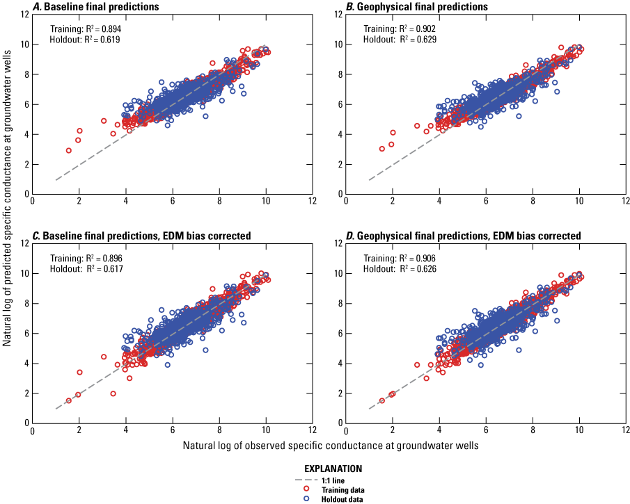
Comparison of observed and predicted specific conductance values at groundwater wells by training and holdout datasets with coefficient of determination (R2) for the final A, baseline and B, geophysical models and for the final C, baseline and D, geophysical models bias corrected with the empirical distribution matching (EDM) method for specific conductance data collected 1942–2020 in the Mississippi Alluvial Plain region. Data from U.S. Geological Survey (2021) and Killian and Knierim (2023).
Overall BRT model performance, reported as coefficient of determination (R2) and RMSE, was similar for the baseline and geophysical models (fig. 5, table 2). The EDM bias-corrected baseline model training R2 and holdout R2 values were 0.896 and 0.617, and the EDM bias-corrected geophysical model training R2 and holdout R2 were 0.906 and 0.626 (fig. 5) (Killian and Knierim, 2023). There was a slight increase in model accuracy based on R2 value of holdout data for the geophysical model (fig. 5). Training data predictions generally had higher accuracy (lower RMSE) than did holdout data predictions, which is typical for BRT models. Training data accuracy is typically higher than holdout data accuracy because training data were used to develop the model and holdout data were used to assess how well the model can predict using new data. Holdout RMSE values ranged from 0.42 to 0.45 (table 2) (Killian and Knierim, 2023).
Table 2.
Hyperparameters for boosted regression tree (BRT) model type for the empirical distribution matching (EDM) bias-corrected, final (variable-reduced), favorite, and best training models for predicting specific conductance at groundwater wells in the Mississippi Alluvial Plain region.[Datasets from U.S. Geological Survey (2021) and Killian and Knierim (2023). n, number of samples; no. explanatory vars, number of explanatory variables; id, interaction depth; mo, minimum number of observations per node; sh, shrinkage; nt, number of trees; RMSE, root-mean-square error]
Each Mississippi Alluvial Plain subregion had a different number of SC measurements, and the range and accuracy of SC predictions varied by subregion (fig. 6). Training R2 values were similar among subregions, ranging from 0.79 to 0.92 (Killian and Knierim, 2023). Holdout R2 values ranged from 0.26 to 0.88 (Killian and Knierim, 2023). The geophysical model had a higher R2 value than the baseline model for the holdout data for all subregions except the Atchafalaya and Grand Prairie. Holdout R2 values for both models were closest in the Delta subregion, where the models had the highest number of SC measurements. Holdout R2 values were highest for both models in the Boeuf subregion. The Saint Francis subregion had the lowest holdout R2 value for the baseline model, where SC is generally lower relative to the rest of the dataset. The Atchafalaya subregion had the lowest holdout R2 value for the geophysical model. Holdout R2 values differed the most in the Deltaic and Chenier Plains subregion, where SC is highest and the number of observations is lowest.
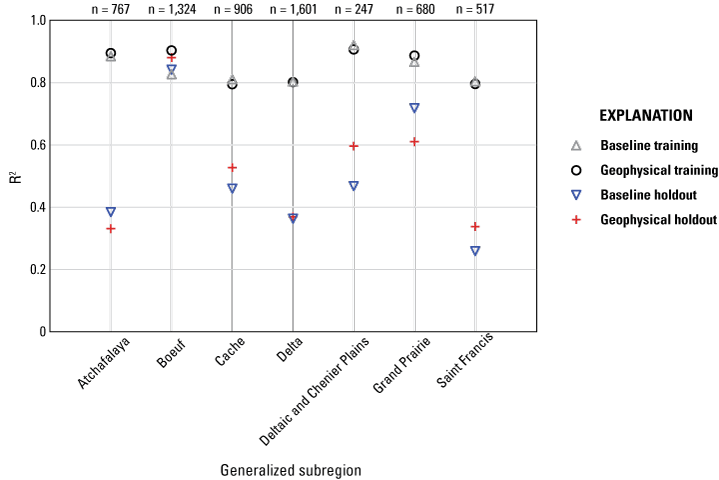
Baseline and geophysical model training and holdout coefficients of determination (R2) values for predictions of specific conductance at groundwater wells by generalized subregion of the Mississippi Alluvial Plain region. Model datasets (1942–2020) from U.S. Geological Survey (2021) and Killian and Knierim (2023); n, number of samples.
When the models are compared by depth slice, SC predictions tend to be higher and more accurate for the geophysical model compared to the baseline model. Holdout R2 values generally increased with depth for both models (fig. 7). Both models also had holdout R2 values less than 0.2 for wells in the 20-ft depth slice (0–20 ft below land surface). Wells less than 20 ft deep (that is, closest to the water table) were the least well defined (n = 78 wells). The geophysical holdout had a higher R2 value compared to the baseline holdout for all depths except for wells in the 75-ft depth slice.
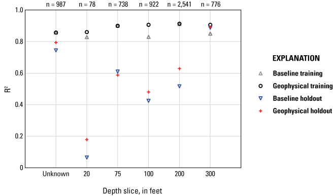
Baseline and geophysical model training and holdout coefficients of determination (R2) values for predictions of specific conductance by depth slice at groundwater wells in the Mississippi Alluvial Plain region. Model datasets (1942–2020) from U.S. Geological Survey (2021) and Killian and Knierim (2023); n, number of samples.
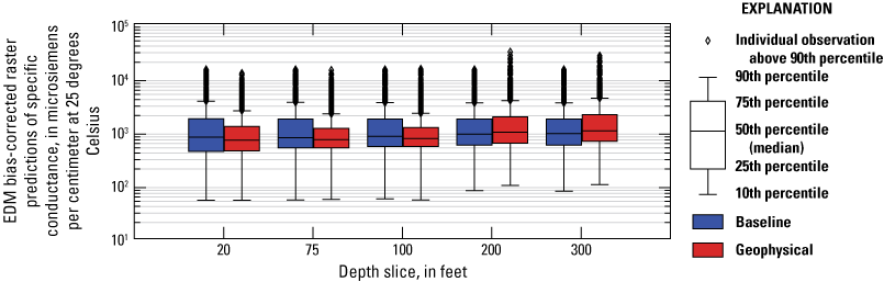
The geophysical model tended to predict higher maximum SC values at each depth slice compared to the baseline model, ranging from 30 to 200 µS/cm higher, although the median predictions were nearly identical (fig. 8A). Once the models were bias corrected using the EDM method, the difference in maximum predictions among depth slices between the baseline and geophysical models was less noticeable (fig. 8B). Therefore, the geophysical explanatory variables may provide additional information to the BRT model to predict high SC values prior to bias correction.
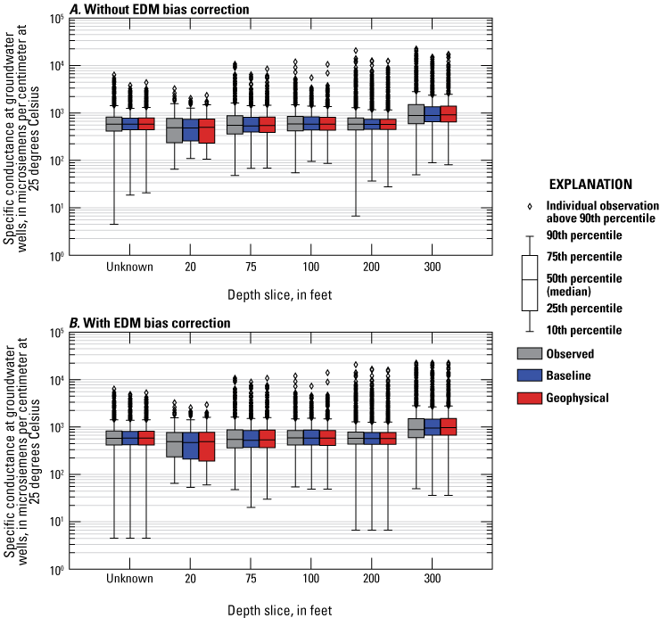
Observed specific conductance 1942–2020 at groundwater wells in the Mississippi Alluvial Plain region (U.S. Geological Survey, 2021; Killian and Knierim, 2023) by depth slice with predictions of specific conductance from the baseline and geophysical models A, without and B, with bias correction using the empirical distribution matching (EDM) method (boxplots created with Python seaborn package [Waskom and others, 2021]).
SC Raster Predictions and Uncertainty
Both the baseline and geophysical models predicted a general increase in SC from north to south, with the highest SC around the Gulf of Mexico (pl. 1). Additionally, both models predicted high SC in areas of known high salinity: around Iberville Parish, La. (Welch and Hanor, 2011); in southeastern Arkansas (Larsen and others, 2021); and around White County, Ark. (Bryant and others, 1985) (figs. 1, 3). The baseline model predicted higher SC near the Gulf of Mexico compared to the geophysical model; frequency of predictions increased between 5,000.1 and 28,000.0 µS/cm in the baseline model (pl. 1, A). The geophysical explanatory variables do not extend to the Gulf of Mexico (figs. 3, 4), so a true one-to-one evaluation of model predictions cannot be quantified. However, a one-to-one comparison of models with identical explanatory variable extents coincident with AEM survey data coverage was explored, and no significant impacts to model performance were discovered because of the nature of how BRT models function. The comparison between models with differing explanatory variable extents was sufficient to assess the impact of AEM survey data on the model, as well as to assess the ability of a BRT model to predict where explanatory variable data are lacking. The extent of AEM survey data coverage created a horizontal linear feature in the geophysical model for all depth predictions (pl. 1, B). The difference in predictions between the baseline and geophysical models increased at the 200- and 300-ft depth slices compared to shallower predictions (pl. 1, C).
The geophysical model predicted higher SC with increasing depth compared to the baseline model, especially above 31 degrees north latitude, where the geophysical datasets were collected (figs. 8, 9, pl. 1). For the 20-, 75-, and 100-ft depth slices, the baseline model predicted a larger interquartile range and higher median than did the geophysical model (fig. 9). The interquartile ranges for the 200- and 300-ft depth slices for both models were similar, but the geophysical model had higher medians and ranges of predictions (fig. 9). This difference between the baseline and geophysical model predictions is more noticeable in areas of known high SC where geophysical explanatory variables are complete (that is, no missing data), such as southeastern Arkansas and northeastern Louisiana (pl. 1).
Raster predictions of specific conductance at groundwater wells in the Mississippi Alluvial Plain region by depth slice for the baseline and geophysical models (boxplots created with Python seaborn package [Waskom and others, 2021]). Model datasets (1942–2020) from U.S. Geological Survey (2021) and Killian and Knierim (2023); EDM, empirical distribution matching.
Uncertainty in SC predictions was high where observed SC was high and where there was a greater range in SC predictions among all 1SE models in both the baseline and geophysical models (fig. 10A, B). High relative uncertainty where the response variable is high has been noted in other ML models (Knierim and others, 2020). The importance of quantifying uncertainty in model predictions depends on how the predictions will be used; for example, whether the modeling effort is focused on accuracy for low or high observed values. High groundwater salinity can limit drinking water and irrigation uses; therefore, qualitative uncertainty was mapped to show where the model is very likely or likely to predict greater or less than the brackish groundwater threshold of 1,000 ppm TDS (fig. 10C, D) (U.S. Geological Survey, 2013). Overall, there were few areas where either model does not predict fresh versus brackish groundwater with a high level of confidence. Confidence was determined by whether the 5th percentile (considered the lowest prediction), median, and 95th percentile (considered the highest prediction) all predicted SC greater or less than 1,000 ppm TDS.
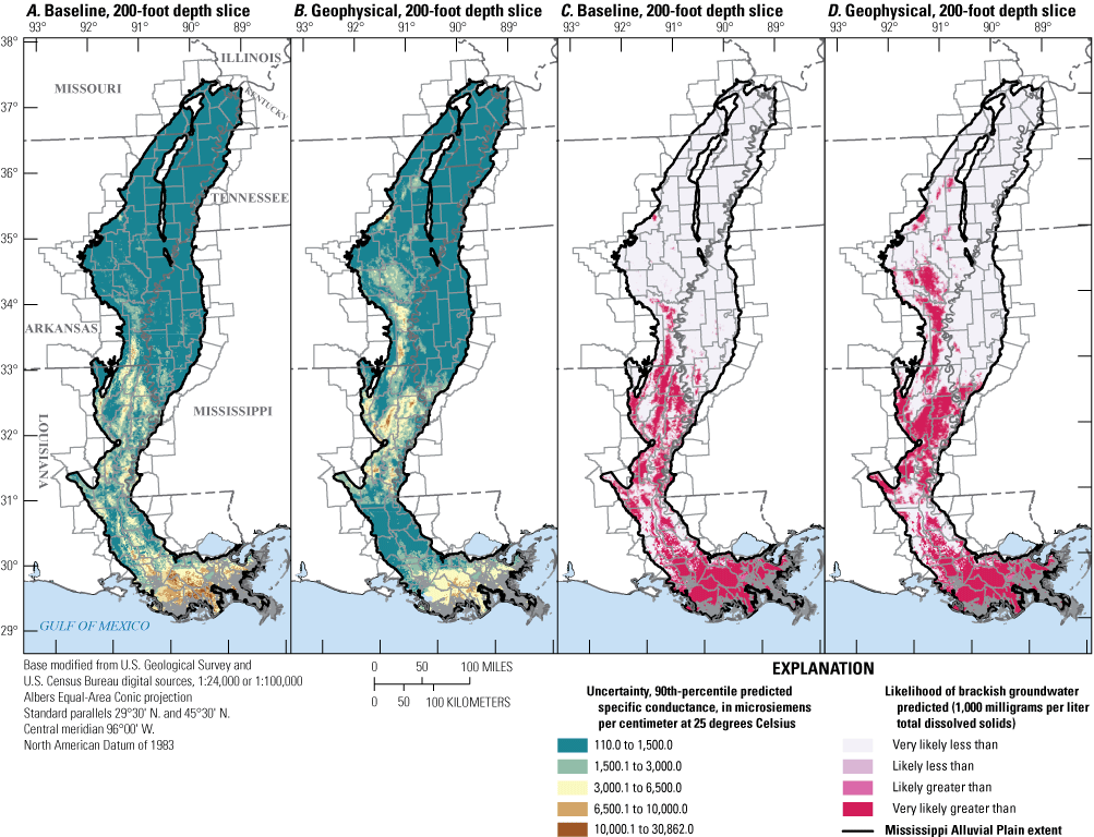
Quantification of specific conductance prediction uncertainty at the 200-foot depth slice for the A, baseline and B, geophysical models and likelihood of brackish groundwater (U.S. Geological Survey, 2013) predicted at the 200-foot depth slice by the C, baseline and D, geophysical models for the Mississippi Alluvial Plain region.
Explanatory Variable Influence
Both the baseline and geophysical models had fewer explanatory variables in the final model compared to the potential explanatory variables used in initial model tuning (table 2). Twenty-two of the 29 explanatory variables were more important than noise and retained in the final baseline model (fig. 11A). The geophysical data added 19 potential explanatory variables. Thirty-three of the 48 explanatory variables, including 12 explanatory variables from the AEM survey, were more important than noise and retained in the final geophysical model (fig. 11B). The same six explanatory variables were found to be less influential than noise in both models, including variables that describe soil texture and the age of surficial sediments (fig. 11).
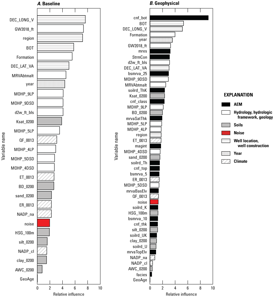
Relative influence of explanatory variables in the A, baseline model (excluding aerial electromagnetic [AEM] explanatory variables) and B, geophysical model (including AEM explanatory variables) for predicting groundwater specific conductance at wells in the Mississippi Alluvial Plain region. The noise variable and all explanatory variables below noise were removed from the final models. See table 1 (at back of report) for descriptions and units of variables.
PDPs for continuous explanatory variables shared between both models show a similar pattern for predicting SC (fig. 12). For example, SC was predicted to be lowest at approximately −92 degrees longitude and highest at approximately −91 degrees longitude in both models (fig. 12E), despite longitude being the first and third influential for the baseline and geophysical models, respectively (fig. 11). The baseline model PDPs generally predicted a higher range of SC than did the geophysical model PDPs for the shared explanatory variables (fig. 12). The depth of the well screen (BOT) was one explanatory variable that showed a different relation between the two models; SC increased with depth in the baseline model and decreased with depth in the geophysical model (fig. 12B). Eleven continuous explanatory variables (fig. 12U–AE) were unique to the geophysical model, and the variable with the largest range of SC predictions was mres (fig. 12Z).
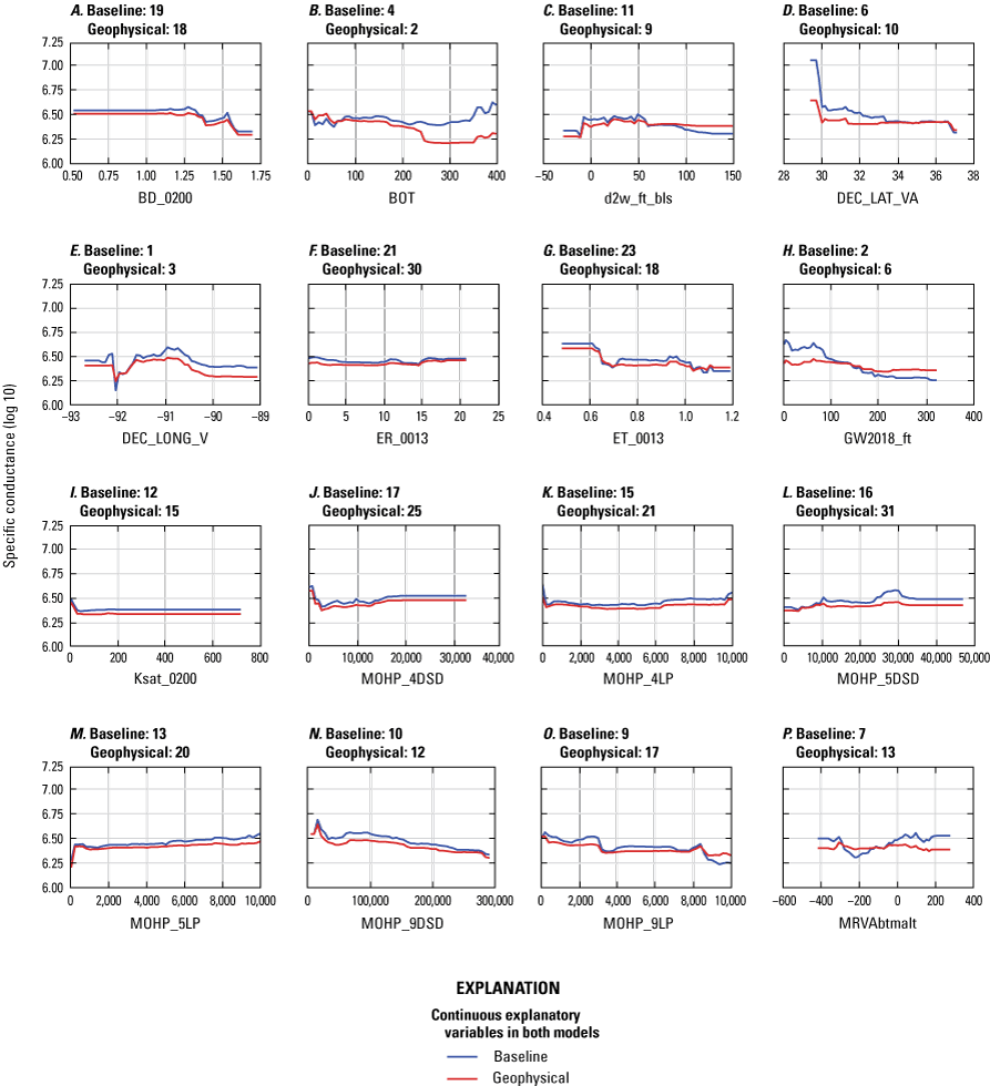
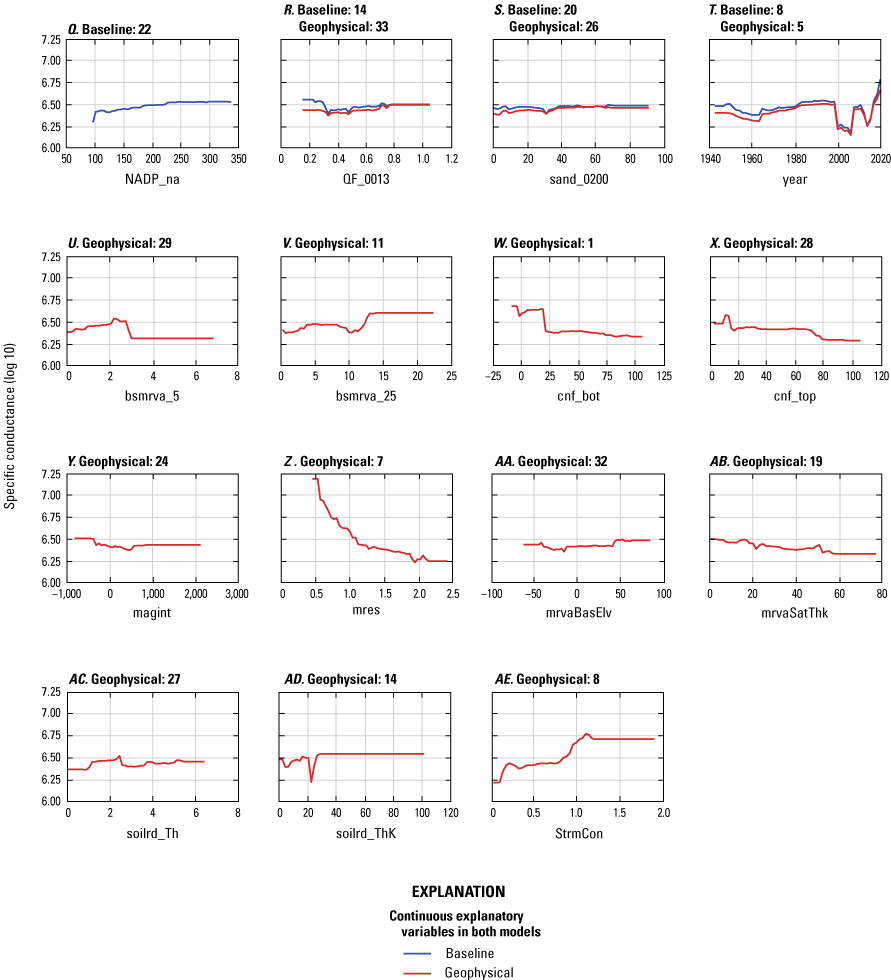
Partial dependence plots of continuous explanatory variables used in the final baseline and geophysical models for predicting groundwater specific conductance at wells in the Mississippi Alluvial Plain region. Numbers in individual graph titles indicate the relative influence ranking of the variable (fig. 11). See table 1 (at back of report) for explanatory variable definitions and units.
Discussion
This section discusses the differences and similarities between the predictions of the baseline and geophysical models. Additionally, the model results are discussed in the context of interpretations of the sources of salinity within the Mississippi Alluvial Plain region.
Missing Data Versus Structured Nulls in BRT Models
BRT models can make predictions even where explanatory variables are missing data because the decision trees are built with the missing data, or null values. Both the baseline and geophysical models were able to predict SC in the southern part of the Mississippi Alluvial Plain region, where there were fewer SC observations (fig. 3, pl. 1). In addition to the paucity of SC observations, geophysical data were not collected below approximately 31 degrees north latitude in the Mississippi Alluvial Plain region prior to or during model development (figs. 3, 4); therefore, there is a large area of nonrandomly distributed (or “structured”) nulls. Because overall model performance was not impacted by the presence of a structured null, as assessed by a one-to-one model comparison with identical extents not described herein, the ability of a BRT model to predict with a structured null as a result of differing explanatory variable extents was tested. For wells in this area, the geophysical model had fewer explanatory variables on which to train. The large structured null created a linear feature in SC predictions for the geophysical model at approximately 31 degrees north latitude (pl. 1, B). Although BRT models can make predictions where there are randomly distributed missing data in explanatory variables, the BRT models do not appear to compensate for structured nulls.
SC was predicted to be lower in the geophysical model relative to the baseline model in the southern extent of the study area (pl. 1), despite the general trend of increasing observed SC toward the Gulf of Mexico (fig. 3). SC predictions north of the linear horizontal feature created by the structured null for the geophysical model were similar between the two models up to approximately the 200-ft depth slice (pl. 1). It cannot be determined which model would predict higher SC in the southern part of the Mississippi Alluvial Plain region if geophysical data were available for the full extent. Although predictive performance is similar between the two models in the Deltaic and Chenier Plains subregion (fig. 6), SC predictions from the geophysical model are likely not reasonable because of the large structured null coincident with missing geophysical explanatory variables.
Position in the Groundwater System Influences SC
The most influential explanatory variables for both the baseline and geophysical models indicate that position in the groundwater system is an important predictor of SC across the Mississippi Alluvial Plain region (fig. 11). A similar result was observed in a previous study in the Mississippi Alluvial Plain region where surrogates for position along groundwater flow paths were important predictors of SC and chloride (Knierim and others, 2020).
The top three most influential explanatory variables for the baseline model (DEC_LONG_V, GW2018_ft, and region [subregion]) are indicators for position in the groundwater system (fig. 11A). SC was predicted to be highest at approximately −91 degrees longitude (fig. 13A), which is the approximate center of the Mississippi Alluvial Plain and where the alluvial aquifer tends to be thickest (Clark and others, 2011). The 2018 alluvial aquifer potentiometric surface (fig. 13C) also reflects position in the system because groundwater altitude is higher in the northern part of the Mississippi Alluvial Plain region, where land surface altitudes are higher compared to sea level. SC was predicted to be high where the potentiometric surface is low (fig. 13C), which occurs toward the Gulf of Mexico. A similar north-to-south trend of increasing SC toward the Gulf of Mexico is evident in SC observations and mapped predictions (fig. 3, pl. 1). SC was also influenced by the subregion where the SC measurement was collected (figs. 11A, 13). The southernmost subregion, the Deltaic and Chenier Plains, tends to have higher SC because of saltwater influence from the Gulf of Mexico (Welch and Hanor, 2011).
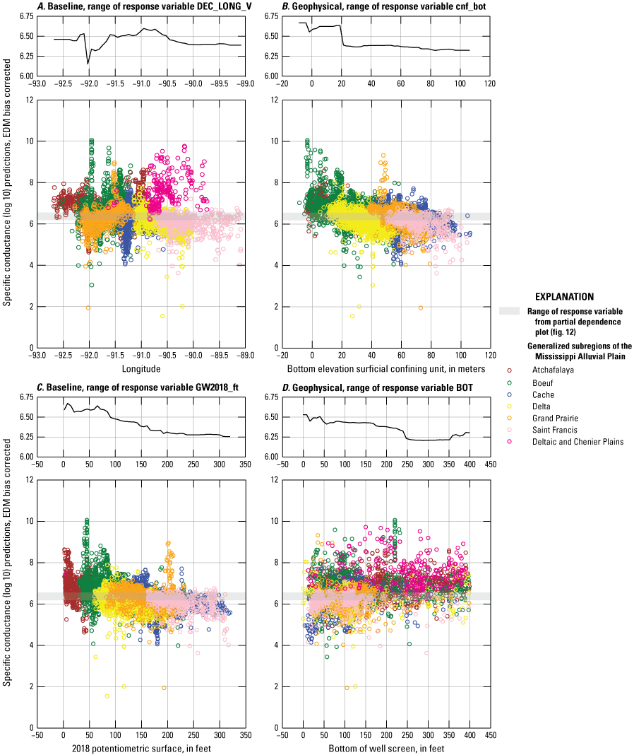
Comparison of the most influential explanatory variables in the A, baseline and B, geophysical models and the second most influential explanatory variables in the C, baseline and D, geophysical models and specific conductance predictions by subregion at groundwater wells in the Mississippi Alluvial Plain region. See table 1 (at back of report) for explanatory variable definitions and units; EDM, empirical distribution matching.
The geophysical model was also influenced by explanatory variables that describe position in the groundwater system. For the geophysical model, the most influential explanatory variable was the bottom altitude of the surficial confining material (cnf_bot) (fig. 11B). Like groundwater altitude, the altitude of the bottom of surficial confining material tends to mimic land surface altitude and decreases from north to south. SC was predicted to be higher where the cnf_bot altitude was low, between 0 and 20 m (fig. 13B), which occurs in the southern half of the Boeuf and Delta subregions. The second most influential explanatory variable for the geophysical model was the bottom of the well screen relative to land surface (BOT) (fig. 13D). Generally, SC would be expected to increase along groundwater flow paths because dissolved solids increase with greater rock-water interaction; depth can serve as a surrogate for flow path (Moore and others, 2019). However, the geophysical model predicted lower SC with increasing well bottom screen depth, which is opposite of the baseline model (fig. 12B) (see below for discussion).
Variation in Model Performance and SC Predictions With Depth
The baseline and geophysical BRT models had similar overall predictive performance despite being tuned with different explanatory variables (tables 1, 2, figs. 5, 7, 11). The predictive performance of both models was also similar to a previous study that predicted SC by using a BRT model in a smaller part of the study area (Knierim and others, 2020). The poor model performance at the 20-ft depth slice (n = 78) may be explained by the lack of SC observations near the water table and thus a lack of training data (fig. 7). Because of the poor model performance at this depth slice, the 20-ft depth prediction is likely inaccurate. More SC observations near the water table would be required to increase prediction accuracy at shallow depths; with the current training data, the BRT models should not be used to make predictions less than 75 ft deep.
Overall, the baseline model predicted similar SC at wells for all depth slices and across all raster depth slices, whereas the geophysical model predicted increasing median SC with depth at wells and raster depth slices (figs. 8, 9, pl. 1). Observed SC was not different among most depth slices, except for higher SC at the 300-ft depth slice (fig. 8), which likely includes wells below the alluvial aquifer. The baseline model included explanatory variables that predominantly describe surficial conditions across the Mississippi Alluvial Plain region (such as multi-order hydrologic position or soils) or two-dimensional position in the system (fig. 11A). BOT was the only three-dimensional explanatory variable in the baseline model and was an important predictor in both models (fig. 11). The geophysical model incorporated additional three-dimensional data including mres measurements that vary with depth within the system (figs. 4, 11B). With the addition of geophysical data, surficial variables decreased in importance in the geophysical model, but position in the groundwater system was still the predominant driving predictor of SC in the Mississippi Alluvial Plain region (fig. 11B). The addition of three-dimensional data in the geophysical model may explain why the median SC predictions at the 200- and 300-ft depth slices are higher than in the baseline model (fig. 9, pl. 1).
The PDPs for BOT show contrasting behavior between models in comparison to mapped predictions; SC was predicted to increase with well screen bottom depth in the baseline model, but it decreases in the geophysical model (fig. 12B). This contrasting relation may be related to the structured nulls in the geophysical model, which led to generally lower SC predictions in the geophysical model compared to the baseline model south of the geophysical data extent (pl. 1). Each PDP provides SC predictions if all other explanatory variables are held at their measured or observed values, except for BOT. The mapped predictions integrate spatial changes in all explanatory variables. Therefore, the BOT explanatory variable may modify the influence of other explanatory variables in predicting SC differently between the models. If AEM geophysical data were available for the entire Mississippi Alluvial Plain extent, the BOT PDP for the geophysical model may display a trend similar to that for the baseline model.
Geophysical Model Explanatory Variables and Sources of Salinity
Areas of elevated SC in the Mississippi Alluvial Plain region have been suggested to be controlled by several possible sources of salinity, including ocean water; salt domes; connection with deeper, more saline subcropping aquifers; or surficial concentration through evaporation in areas of low infiltration controlled by the presence or absence of surficial confining units (Pettijohn and others, 1988; Williamson and others, 1990; Kresse and Clark, 2008; Kingsbury and others, 2014). The north-to-south trend of increasing SC observations and predictions illustrates that ocean water influences groundwater SC in the southern part of the study area close to the Gulf of Mexico (pl. 1, callouts 3 and 6). Salt domes were not included as an explanatory variable and so were not tested as a source of salinity in the BRT models. The addition of geophysical explanatory variables added three-dimensional information about hydrogeology, including the location and thickness of confining units at the surface and with depth (James and Minsley, 2021; Minsley and others, 2021), that was unavailable to the baseline model. These additional variables allowed exploration of how surficial confinement or connection with deeper units may influence SC.
Effects of Deeper Saline Aquifers on Salinity in the Alluvial Aquifer
High SC may occur in the alluvial aquifer where there is a deeper source of salinity in connection with the alluvial aquifer (Kresse and Clark, 2008; Larsen and others, 2021). The bsmrva_25 geophysical explanatory variable is an estimation of the vertical hydraulic connectivity 25 m above and below the base of the alluvial aquifer; high values indicate poor hydraulic connection (James and Minsley, 2021) (fig. 12V). In contrast to conceptual models, the geophysical model predicted high SC where bsmrva_25 was high (fig. 12V), which corresponds to low mres and indicates that fine-grained sediments may be present (fig. 4). Broad areas of high predicted SC in southeastern Arkansas and northeastern Louisiana are coincident with the subcropping Vicksburg-Jackson confining unit (pl. 1). This area includes observations of high SC groundwater and good model performance in the Boeuf subregion (fig. 6). Specifically in Chicot County, Ark. (fig. 3), high SC occurs in an area where mres suggests that coarser grained sediments may be present and bsmrva_25 suggests that the alluvial aquifer may be connected with deeper, more saline aquifers; however, this pattern is not evident for the entire study area. The geophysical model may be predicting high SC where confining units are present because the resistivity signal captures both aquifer and porewater resistivity. For example, in northeastern Arkansas, high SC predictions are coincident with an area where bsmrva_25 is high (pl. 1, callouts 1 and 4); however, high SC observations are only localized around the Bald Knob, Ark., area (fig. 3). The geophysical model may be conflating the pattern of high SC and confining units in some areas of the model, thus causing overprediction of SC in other areas and increasing the difference in predictions between the two models (pl. 1).
Effects of Surficial Confining Characteristics on Salinity in the Alluvial Aquifer
The presence or absence of a surficial confining unit has been hypothesized to control salinity in some areas of the alluvial aquifer (Kresse and Clark, 2008). The absence, presence, and thickness of the surficial confining unit were represented by several geophysical explanatory variables, including cnf_top, cnf_bot, cnf_class, and cnf_thk (table 1, at back of report). As discussed in the “Discussion” section, cnf_top (fig. 12X) and cnf_bot (fig. 12W) are more representative of position in the groundwater system in the geophysical BRT model than is cnf_class. The geophysical model did not find cnf_thk to be an important predictor of SC (fig. 11). Cnf_class, a categorical variable, represents the degree of surficial confinement and was the 16th most influential explanatory variable. Low cnf_class categories correspond to fine-grained, low-permeability materials (James and Minsley, 2021). Low cnf_class categories were predicted to have higher SC than high cnf_class categories, though the variation was small (Killian and Knierim, 2023).
Relative Influences of Lithology and Salinity
Mres at the midpoint of the well screen was the seventh most influential explanatory variable in the geophysical model (fig. 11B). Mres captures both aquifer properties and porewater salinity, and previous analysis of the Mississippi Alluvial Plain region has shown that saline groundwater can influence resistivity measurements (Minsley and others, 2021). There is an inverse relation between SC and resistivity (fig. 14). Therefore, the geophysical model provides additional evidence that mres includes a resistivity signal driven, in part, by high SC (or saline) groundwater (fig. 14). Mres provides important three-dimensional information to the geophysical model and can be used to delineate contacts between the alluvial aquifer and deeper Tertiary confining units or aquifers (figs. 1, 4). However, because of the presence of saline groundwater in some areas of the alluvial aquifer (fig. 3), low mres (or high conductance) signals in the AEM survey data are not well constrained (Ward, 1990; Hilmi and Madun, 2022). Low resistivity can be the result of high salinity, the presence of fine-grained lithology, or a combination of the two (Zohdy and others, 1974). More work is needed to resolve the groundwater SC (salinity) signal within AEM-derived resistivity data across the Mississippi Alluvial Plain region. Removing the salinity signal could allow for better estimation of subsurface materials, thus allowing for more accurate estimates of available water resources.
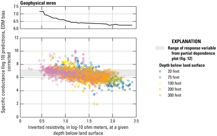
Comparison of inverted resistivity (mres) and specific conductance predictions for a given depth below land surface at groundwater wells in the Mississippi Alluvial Plain region by the geophysical model. See table 1 (at back of report) for explanatory variable definitions and units; EDM, empirical distribution matching.
Lack of Temporal SC Variations at Wells
The year an SC measurement was collected was included as an explanatory variable in both models and had a similar influence on SC predictions (fig. 11). The SC dataset includes sampling networks from six States and includes long-term State cooperative programs to monitor salinity in Louisiana and Arkansas (Killian and Knierim, 2023), but network sampling priorities have changed over time, and there are gaps in the spatial and temporal coverage of data. For example, the Deltaic and Chenier Plains subregion shows elevated SC (fig. 3) but lacks data compared to other subregions (fig. 2A). Most SC measurements in this subregion were made prior to the year 1980 (fig. 2A). In contrast, there was an increase in SC observations after 1980 in the Delta subregion (fig. 2A). There may also be a bias introduced from networks that have the goal of monitoring localized high-salinity areas. The importance of this explanatory variable is likely driven by differences in sampling networks, as opposed to the BRT models capturing systematic changes in SC conditions throughout the aquifer.
In addition to the variation in the sampling network over time, groundwater quality may change at a location as water is withdrawn for irrigation or the aquifer is recharged (Kingsbury and others, 2014; Jurgens and others, 2020). Because only the most recent sample was used if a well had more than one observation, the model was not given information about how SC changed over time at a well. The SC maps were predicted using the year 2018 because 2018 was coincident with data collection for several explanatory variables. Although SC prediction maps could be made for any specified year, it would not be appropriate to use the maps to evaluate SC change through time across the aquifer. To understand how SC changes through time and which explanatory variables drive the change, explanatory variables that capture these changes through time are needed in addition to time-series SC observations.
Uncertainty in High SC in the Mississippi Alluvial Plain Region
The baseline and geophysical models showed overall similar trends in predicting broad areas of low SC in the northern part of the Mississippi Alluvial Plain region and high SC from southeastern Arkansas to the Gulf of Mexico (pl. 1). There are also several areas of localized known high SC in the Mississippi Alluvial Plain region (fig. 3), and both models were able to predict elevated SC in these areas (pl. 1). However, the spatial extent and magnitude of SC predictions were different between the baseline and geophysical models (pl. 1). Depending on which model is used, the same location can be predicted with high confidence to have either fresh or brackish groundwater. For example, the Grand Prairie subregion (fig. 1) is predicted to have more brackish groundwater in the geophysical model than in the baseline model (fig. 10). Both models have similar overall accuracy (fig. 5) and similar accuracy among prediction depth ranges (fig. 7) and subregions (fig. 6). Therefore, both models have a similar magnitude of overpredicting or underpredicting SC across the Mississippi Alluvial Plain region (fig. 5).
The appropriate model and prediction maps to use depend on the goal and area for assessing SC conditions. Both models showed poor prediction accuracy for shallow SC conditions (fig. 7). SC predictions near the Gulf of Mexico from the geophysical model may not be realistic because of the structured nulls in training data (fig. 6, pl. 1). Additionally, the high SC predictions in northeastern Arkansas from the geophysical model may be spurious because of the lack of high SC observations in that area. In contrast, the baseline model was trained with no three-dimensional data other than well depth, so the geophysical model may be more appropriate to use when making deeper SC predictions (fig. 7). Both the baseline and geophysical models can make accurate SC predictions for the Mississippi Alluvial Plain region with the given input data, but model outputs should be selected and interpreted on the basis of the scientific goal.
Summary
Groundwater is an important source of freshwater for agriculture and drinking water in the United States and around the world. Elevated specific conductance (SC) in aquifers can limit where freshwater is available for use. The Mississippi Alluvial Plain region is a major source of groundwater for irrigation in the south-central United States and includes areas of high SC that limit use. In 2021, the U.S. Geological Survey trained two boosted regression tree (BRT) machine-learning models on SC data available between 1942 and 2020 to predict groundwater SC across the Mississippi Alluvial Plain region at multiple depths below land surface for the Mississippi River Valley alluvial and deeper aquifers. Two BRT models were created, a baseline model and a geophysical model, to test and evaluate how the incorporation of aerial electromagnetic (AEM) data from an aquifer-wide geophysical survey affected model predictive performance and sensitivity. Geophysical data provided information about the three-dimensional hydrogeologic properties of aquifers and confining units, which affect groundwater flow paths and geochemistry.
The BRT models were developed using SC measurements collected at wells between 1942 and 2020, and predictions were made at a 1-kilometer resolution at multiple depths. Final models included explanatory variables that were more influential than random noise. The final baseline model was trained with 22 of the 29 available explanatory variables, which predominantly represented surficial information. The final geophysical model incorporated geophysical data from a regional AEM survey and was trained on 33 of the 48 available explanatory variables. Twelve of the explanatory variables in the final geophysical model were from the AEM survey. Explanatory variables that describe position in the groundwater system were important drivers of SC for both models. Both models accurately predicted SC across the Mississippi Alluvial Plain region and corresponded to observed SC; the bias-corrected baseline model training coefficient of determination (R2) value and holdout R2 value were 0.896 and 0.617, and the bias-corrected geophysical model training R2 value and holdout R2 value were 0.906 and 0.626, respectively. Both models were able to predict elevated SC in known areas of high SC. The addition of AEM survey data did not improve the model globally, likely because of how effective BRT models are at identifying patterns in data. When the baseline and geophysical models are compared by region and depth, however, there is improvement in the geophysical model. AEM survey data provided additional three-dimensional information, whereas the baseline model relied on surficial variables and well depth to predict salinity at depth.
The models help to predict the extent of areas with elevated SC both vertically and horizontally for the Mississippi Alluvial Plain region. The baseline and geophysical models predicted similar areas of low SC in the northern part of the Mississippi Alluvial Plain region and high SC from southeastern Arkansas to the Gulf of Mexico. Geophysical data were available for the northern part of the study area and did not extend to the Gulf of Mexico. The missing geophysical explanatory variables for the southern part of the study area caused a linear artifact in SC predictions in the geophysical model. Therefore, BRT models can make predictions where explanatory variables are missing but cannot compensate for large areas of missing data (structured nulls). Because of the lack of geophysical explanatory variables for the southern part of the study area, SC predictions by the geophysical model are likely unreliable in that area. The geophysical data provided three-dimensional information that the baseline model did not have, which caused the geophysical model to predict greater SC with depth. Machine-learning models are useful for predicting groundwater quality in unmonitored locations at the regional scale, but model limitations and prediction uncertainty should be considered within the context appropriate for the system and scientific goals.
Table 1.
Name, unit, description, dataset group, and source information for each variable in the baseline and geophysical models to predict groundwater specific conductance across the Mississippi Alluvial Plain region.[NA, not applicable; cm, centimeter; mm, millimeter; m, meter; +/−, above and below; AEM, aerial electromagnetic; NAD 83, North American Datum of 1983; mm/dd/yyyy hh:mm, month/day/year hour:minute; NAVD 88, North American Vertical Datum of 1988; xml, Extensible Markup Language; km, kilometer; yyyy, year; EDM, empirical distribution matching]
| Name | Units or format | Description | Final baseline model variable | Final geophysical model variable | Dataset group | Citation |
|---|---|---|---|---|---|---|
| SITEAG | NA | Well identifier | NA | NA | Supplementary information | U.S. Geological Survey (2021) |
| AQFR_CD | eight-character string | Aquifer code (from https://help.waterdata.usgs.gov/aqfr_cd#:~:text=Aquifer%20Codes%20(aqfr_cd),by%20the%20Water%20Resources%20Division.%22) | NA | NA | Supplementary information | U.S. Geological Survey (2021) |
| AWC_0200 | inches per foot | Available water capacity (AWC), quantity of water soil can store for use by plants, 0 to 200 cm depth | No | No | Input, explanatory variable, soils | Soil Survey Staff (2020) |
| BD_0200 | grams per cubic centimeter | Bulk density (BD), oven-dried weight of the soil material less than 2 mm in size per unit volume of soil at water tension of 1/3 bar, 0 to 200 cm depth | Yes | Yes | Input, explanatory variable, soils | Soil Survey Staff (2020) |
| bsmrva_5 | 5 m +/− the Mississippi River Valley alluvial aquifer base | Vertically integrated electrical conductance values within the vertical interval spanning +/− 5 m across the base of the Mississippi River Valley alluvial aquifer | NA | Yes | Input, explanatory variable, AEM | James and Minsley (2021) |
| bsmrva_10 | 10 m +/− the Mississippi River Valley alluvial aquifer base | Vertically integrated electrical conductance values within the vertical interval spanning +/− 10 m across the base of the Mississippi River Valley alluvial aquifer | NA | No | Input, explanatory variable, AEM | James and Minsley (2021) |
| bsmrva_25 | 25 m +/− the Mississippi River Valley alluvial aquifer base | Vertically integrated electrical conductance values within the vertical interval spanning +/− 25 m across the base of the Mississippi River Valley alluvial aquifer | NA | Yes | Input, explanatory variable, AEM | James and Minsley (2021) |
| BOT | feet | Bottom of well screen | Yes | Yes | Input, explanatory variable, well construction | U.S. Geological Survey (2021) |
| clay_0200 | percentage | Clay, soil separate consists of mineral soil particles that are less than 0.002 mm in diameter, 0 to 200 cm depth | No | No | Input, explanatory variable, soils | Soil Survey Staff (2020) |
| cnf_bot | meters | Bottom altitude corresponding to the surficial confining material of the Mississippi River Valley alluvial aquifer | NA | Yes | Input, explanatory variable, AEM | James and Minsley (2021) |
| cnf_class | category −3 to 3 | Metric representing the degree of surface confinement or connectivity that ranges from fully confining conditions to high potential hydrologic connectivity of the Mississippi River Valley alluvial aquifer | NA | Yes | Input, explanatory variable, AEM | James and Minsley (2021) |
| cnf_thk | meters | Occurrence and thickness of surficial (less than 15 m depth) confining material of the Mississippi River Valley alluvial aquifer | NA | No | Input, explanatory variable, AEM | James and Minsley (2021) |
| cnf_top | meters | Top altitude corresponding to the surficial confining material of the Mississippi River Valley alluvial aquifer | NA | Yes | Input, explanatory variable, AEM | James and Minsley (2021) |
| d2w_ft_bls | feet below land surface | Depth to water, spring 2018, Mississippi River Valley alluvial aquifer | Yes | Yes | Input, explanatory variable, hydrology | McGuire and others (2023) |
| DEC_LAT_VA | decimal degrees, NAD 83 | Latitude | Yes | Yes | Input, explanatory variable, location information | U.S. Geological Survey (2021) |
| DEC_LONG_V | decimal degrees, NAD 83 | Longitude | Yes | Yes | Input, explanatory variable, location information | U.S. Geological Survey (2021) |
| dttm | mm/dd/yyyy hh:mm | Date and time stamp of water-quality sample collection | NA | NA | Supplementary information | U.S. Geological Survey (2021) |
| ER_0013 | inches per year | Empirical water balance (EWB) model, estimates of effective recharge, years 2000–13 | Yes | Yes | Input, explanatory variable, climate | Reitz and others (2017a, b) |
| ET_0013 | inches per year | Empirical water balance (EWB) model, estimates of evapotranspiration, years 2000–13 | Yes | Yes | Input, explanatory variable, climate | Reitz and others (2017a, b) |
| facies_[d] | class 0 to 20 | Facies class for materials expected to have similar hydrologic and geologic properties based on electrical resistivity for the depth (d) of interest. For well points, facies class is calculated for the screened interval | NA | No | Input, explanatory variable, AEM | James and Minsley (2021) |
| Formation | formation symbol; see Wacaster and others (2018) for explanation | Saucier geomorphology by formation | Yes | Yes | Input, explanatory variable, geology | Wacaster and others (2018) |
| GeoAge | category | Saucier geomorphology formation grouped by geologic age (Holocene or Pleistocene) | No | No | Input, explanatory variable, geology | Wacaster and others (2018) |
| GW2018_ft | feet, NAVD 88 | Potentiometric surface of the Mississippi River Valley alluvial aquifer for the year 2018 | Yes | Yes | Input, explanatory variable, hydrology | McGuire and others (2020a, b) |
| HSG_100m | character string | Hydrologic soil groups (HSG), classes that indicate runoff potential for soils. See Killian and Knierim (2023) for category description. | No | No | Input, explanatory variable, soils | Soil Survey Staff (2020) |
| Ksat_0200 | inches per day | Saturated hydraulic conductivity (Ksat), ability of a saturated soil to transmit water, 0 to 200 cm depth | Yes | Yes | Input, explanatory variable, soils | Soil Survey Staff (2020) |
| Layer | character string | Flag for group of aquifer codes. See Killian and Knierim (2023) for category description. | NA | NA | Supplementary information | NA |
| ls_alt | feet | Land surface altitude, used to calculate depth of prediction for rasters | No | No | Supplementary information | U.S. Geological Survey (2018) |
| magint | nano Teslas | Residual magnetic intensity | No | Yes | Input, explanatory variable, AEM | Burton and others (2021) |
| MOHP_[i]DSD | meters | Multi-order hydrologic position (MOHP) of ith-order streams, distance to stream divide (DSD) | 9, 5, 4 | 9, 5, 4 | Input, explanatory variable, hydrology | Moore and others (2019), Belitz and others (2019) |
| MOHP_[i]LP | meters | Multi-order hydrologic position (MOHP) of ith-order streams, lateral position (LP) | 9, 5, 4 | 9, 5, 4 | Input, explanatory variable, hydrology | Moore and others (2019), Belitz and others (2019) |
| mres_[d] | log 10 | Inverted resistivity (ohm meters) at a given depth (d) below land surface | NA | Yes | Input, explanatory variable, AEM | James and Minsley (2021), Minsley and others (2021) |
| mrvaBasElv | meters | Mississippi River Valley alluvial aquifer base altitude | NA | Yes | Input, explanatory variable, AEM | James and Minsley (2021) |
| MRVAbtmalt | feet | Bottom of the Mississippi River Valley alluvial aquifer, altitude | Yes | Yes | Input, explanatory variable, hydrogeologic framework | Torak and Painter (2019a, b) |
| mrvaSatThk | meters | Saturated Mississippi River Valley alluvial aquifer thickness | NA | Yes | Input, explanatory variable, AEM | James and Minsley (2021) |
| mrvaTopElv | meters | Top altitude of the saturated Mississippi River Valley alluvial aquifer based on the 2018 potentiometric surface and digital elevation model | NA | No | Input, explanatory variable, AEM | James and Minsley (2021) |
| NADP_cl | milligrams per liter | National Atmospheric Deposition Program (NADP) 26-year average chloride (Cl) concentration | No | No | Input, explanatory variable, climate | National Atmospheric Deposition Program (2021) |
| NADP_na | kilograms per hectare | National Atmospheric Deposition Program (NADP) 26-year average sodium (Na) concentration | Yes | No | Input, explanatory variable, climate | National Atmospheric Deposition Program (2021) |
| NAT_AQFR_C | character string | National aquifer code, reference list available at https://www.usgs.gov/mission-areas/water-resources/science/national-aquifer-code-reference-list | NA | NA | Supplementary information | U.S. Geological Survey (2021) |
| noise | NA | Random noise | No | No | Input, explanatory variable | NA |
| QF_0013 | inches per year | Empirical water balance (EWB) model, estimates of quickflow (runoff), years 2000–13 | Yes | Yes | Input, explanatory variable, climate | Reitz and others (2017a, b) |
| r00095 | less than and greater than the specific conductance value | Flag for censored values | NA | NA | Supplementary information | U.S. Geological Survey (2021) |
| region | see Mississippi Alluvial Plain generalied_regions_FGDC_metadata.xml available at the citation for category description | Seven generalized subregions of the Painter and Westerman (2018) extent of the Mississippi Alluvial Plain to provide a framework for analysis, visualization, and regional comparisons of local data within the region. | Yes | Yes | Input, explanatory variable, location information | Ladd and Travers (2019) |
| sand_0200 | percentage | Sand, soil separate consists of mineral soil particles that are 0.05 to 2 mm in diameter, 0 to 200 cm depth | Yes | Yes | Input, explanatory variable, soils | Soil Survey Staff (2020) |
| SC | microsiemens per centimeter at 25 degrees Celsius | Specific conductance value | NA | NA | Input, response variable | U.S. Geological Survey (2021) |
| silt_0200 | percentage | Silt, soil separate consists of mineral soil particles that are 0.002 to 0.05 mm in diameter, 0 to 200 cm depth | No | No | Input, explanatory variable, soils | Soil Survey Staff (2020) |
| soilrd_K | percentage | Potassium soil radiometrics | NA | No | Input, explanatory variable, AEM | Burton and others (2021) |
| soilrd_Th | parts per million | Thorium (eTh) soil radiometrics | NA | Yes | Input, explanatory variable, AEM | Burton and others (2021) |
| soilrd_ThK | ratio | Soil radiometric ratio of thorium and potassium (rThK) | NA | Yes | Input, explanatory variable, AEM | Burton and others (2021) |
| soilrd_U | parts per million | Uranium (eU) soil radiometrics | NA | No | Input, explanatory variable, AEM | Burton and others (2021) |
| soilrd_UK | ratio | Soil radiometric ratio of uranium and potassium (rUK) | NA | No | Input, explanatory variable, AEM | Burton and others (2021) |
| SOURCE | category | Source of well construction information and water-quality data | NA | NA | Supplementary information | NA |
| StrmCon | siemens | Streambed connectivity, vertically integrated electrical conductance values from 0 to 10 m depth for all locations within 1 km radius of streams within the Mississippi Alluvial Plain region | NA | Yes | Input, explanatory variable, AEM | James and Minsley (2021) |
| subUnit | category | Subcropping hydrogeologic unit | NA | NA | Supplementary information | Hart and others (2008) |
| TOP | feet | Top of well screen | NA | NA | Supplementary information | U.S. Geological Survey (2021) |
| WELL_DEPTH | feet | Depth of well below land surface | NA | NA | Supplementary information | U.S. Geological Survey (2021) |
| year | yyyy | Year sample was collected | Yes | Yes | Input, explanatory variable | U.S. Geological Survey (2021) |
| m1Pred_ln | natural log | Baseline model predicted specific conductance | NA | NA | Output, prediction | Killian and Knierim (2023) |
| m1P_uScm | microsiemens per centimeter | Baseline model predicted specific conductance | NA | NA | Output, prediction | Killian and Knierim (2023) |
| m1edmP_ln | natural log | Predicted specific conductance with EDM bias correction for the baseline model | NA | NA | Output, prediction | Killian and Knierim (2023) |
| m1edmP_uScm | microsiemens per centimeter | Baseline model EDM bias correction for predicted specific conductance, backtransformed to original units | NA | NA | Output, prediction | Killian and Knierim (2023) |
| m1res_uScm | microsiemens per centimeter | Baseline model residuals (observed − predicted specific conductance) | NA | NA | Output, prediction | Killian and Knierim (2023) |
| m1rEDM_uScm | microsiemens per centimeter | Baseline model EDM bias correction of residuals (observed − predicted specific conductance) | NA | NA | Output, prediction | Killian and Knierim (2023) |
| m2Pred_ln | natural log | Geophysical model predicted specific conductance | NA | NA | Output, prediction | Killian and Knierim (2023) |
| m2P_uScm | microsiemens per centimeter | Geophysical model predicted specific conductance | NA | NA | Output, prediction | Killian and Knierim (2023) |
| m2edmP_ln | natural log | Predicted specific conductance with EDM bias correction for the geophysical model | NA | NA | Output, prediction | Killian and Knierim (2023) |
| m2edmP_uScm | microsiemens per centimeter | Geophysical model EDM bias correction of predicted specific conductance, backtransformed to original units | NA | NA | Output, prediction | Killian and Knierim (2023) |
| m2res_uScm | microsiemens per centimeter | Geophysical model residuals (observed − predicted specific conductance) | NA | NA | Output, prediction | Killian and Knierim (2023) |
| m2rEDM_uScm | microsiemens per centimeter | Geophysical model EDM bias correction of residuals (observed − predicted specific conductance) | NA | NA | Output, prediction | Killian and Knierim (2023) |
References Cited
Alhassan, M., Lawrence, C.B., Richardson, S., and Pindilli, E.J., 2019, The Mississippi Alluvial Plain aquifers—An engine for economic activity: U.S. Geological Survey Fact Sheet 2019–3003, accessed January 7, 2022, at https://doi.org/10.3133/fs20193003.
Arslan, H., 2012, Spatial and temporal mapping of groundwater salinity using ordinary kriging and indicator kriging—The case of Bafra Plain, Turkey: Agricultural Water Management, v. 113, p. 57–63. [Also available at https://doi.org/10.1016/j.agwat.2012.06.015.]
Belitz, K., Moore, R.B., Arnold, T.L., Sharpe, J.B., and Starn, J.J., 2019, Multiorder hydrologic position in the conterminous United States—A set of metrics in support of groundwater mapping at regional and national scales: Water Resources Research, v. 55, no. 12, p. 11188–11207, accessed March 21, 2023, at https://doi.org/10.1029/2019WR025908.
Belitz, K., and Stackelberg, P.E., 2021, Evaluation of six methods for correcting bias in estimates from ensemble tree machine learning regression models: Environmental Modelling & Software, v. 139, article 105006, accessed August 26, 2021, at https://doi.org/10.1016/j.envsoft.2021.105006.
Burton, B.L., Minsley, B.J., Bloss, B.R., and Kress, W.H., 2021, Airborne electromagnetic, magnetic, and radiometric survey of the Mississippi Alluvial Plain, November 2018–February 2019: U.S. Geological Survey data release, accessed February 20, 2021, at https://doi.org/10.5066/P9XBBBUU.
Clark, B.R., Barlow, P.M., Peterson, S.M., Hughes, J.D., Reeves, H.W., and Viger, R.J., 2018, National-scale grid to support regional groundwater availability studies and a national hydrogeologic database: U.S. Geological Survey data release, accessed August 23, 2020, at https://doi.org/10.5066/F7P84B24.
Clark, B.R., Hart, R.M., and Gurdak, J.J., 2011, Groundwater availability of the Mississippi embayment: U.S. Geological Survey Professional Paper 1785, 62 p. [Also available at https://doi.org/10.3133/pp1785.]
Clark, B.R., Knierim, K.J., and Duncan, L., 2019, Zonepy—Zonal analysis tools for raster and vector datasets: U.S. Geological Survey software release, accessed August 2, 2021, at https://github.com/brclark-usgs/zonepy.
Delsman, J.R., Van Baaren, E.S., Siemon, B., Dabekaussen, W., Karaoulis, M.C., Pauw, P.S., Vermaas, T., Bootsma, H., de Louw, P.G.B., Gunnink, J.L., Dubelaar, C.W., Menkovic, A., Steuer, A., Meyer, U., Revil, A., and Oude Essink, G.H.P., 2018, Large-scale, probabilistic salinity mapping using airborne electromagnetics for groundwater management in Zeeland, the Netherlands: Environmental Research Letters, v. 13, no. 8, article 084011, accessed February 8, 2022, at https://doi.org/10.1088/1748-9326/aad19e.
Esri, 2020, ArcGIS Desktop, release 10.8: Redlands, Calif., Esri software release, accessed February 2, 2021, at https://www.esri.com.
Goldstein, A., Kapelner, A., Bleich, J., and Pitkin, E., 2015, Peeking inside the black box—Visualizing statistical learning with plots of individual conditional expectation: Journal of Computational and Graphical Statistics, v. 24, no. 1, p. 44–65, accessed November 21, 2022, at https://doi.org/10.1080/10618600.2014.907095.
Greenwell, B.M., 2017, pdp—An R package for constructing partial dependence plots: The R Journal, v. 9, no. 1, p. 421–436, accessed August 23, 2021, at https://journal.r-project.org/archive/2017/RJ-2017-016/index.html.
Hardke, J.T., 2021, Rice production handbook: University of Arkansas Division of Agriculture Cooperative Extension Service MP 192, 214 p., accessed February 10, 2022, at https://www.uaex.uada.edu/publications/pdf/mp192/mp192.pdf.
Hilmi, N.A.S.M., and Madun, A., 2022, The effect of salinity towards resistivity for groundwater interpretation: Recent Trends in Civil Engineering and Built Environment, v. 3, no. 1, p. 1743–1751, accessed March 23, 2023, at https://doi.org/10.30880/rtcebe.2022.03.01.194.
James, S.R., and Minsley, B.J., 2021, Combined results and derivative products of hydrogeologic structure and properties from airborne electromagnetic surveys in the Mississippi Alluvial Plain: U.S. Geological Survey data release, accessed December 12, 2021, at https://doi.org/10.5066/P9382RCI.
Jones, C.E., An, K., Blom, R.G., Kent, J.D., Ivins, E.R., and Bekaert, D., 2016, Anthropogenic and geologic influences on subsidence in the vicinity of New Orleans, Louisiana: Journal of Geophysical Research. Solid Earth, v. 121, no. 5, p. 3867–3887, accessed March 22, 2022, at https://doi.org/10.1002/2015JB012636.
Jurgens, B.C., Fram, M.S., Rutledge, J., and Bennett, G.L., V., 2020, Identifying areas of degrading and improving groundwater-quality conditions in the State of California, USA, 1974–2014: Environmental Monitoring and Assessment, v. 192, article 250, accessed February 7, 2022, at https://doi.org/10.1007/s10661-020-8180-y.
Killian, C.D., Asquith, W.H., Barlow, J.R.B., Bent, G.C., Kress, W.H., Barlow, P.M., and Schmitz, D.W., 2019, Characterizing groundwater and surface-water interaction using hydrograph-separation techniques and groundwater-level data throughout the Mississippi Delta, USA: Hydrogeology Journal, v. 27, no. 6, p. 2167–2179, accessed May 25, 2019, at https://doi.org/10.1007/s10040-019-01981-6.
Killian, C.D., and Knierim, K.J., 2023, Machine-learning model predictions and rasters of groundwater salinity in the Mississippi Alluvial Plain: U.S. Geological Survey data release, https://doi.org/10.5066/P9WSE8JS.
Kingsbury, J.A., Barlow, J.R.B., Katz, B.G., Welch, H.L., Tollett, R.W., and Fahlquist, L.S., 2015, The quality of our Nation’s waters—Water quality in the Mississippi embayment-Texas coastal uplands aquifer system and Mississippi River Valley alluvial aquifer, south-central United States, 1994–2008: U.S. Geological Survey Circular 1356, 72 p., accessed February 7, 2022, at https://doi.org/10.3133/cir1356.
Knierim, K.J., Kingsbury, J.A., Haugh, C.J., and Ransom, K.M., 2020, Using boosted regression tree models to predict salinity in the Mississippi embayment aquifers, central United States: Journal of the American Water Resources Association, v. 56, no. 6, p. 1010–1029, accessed August 26, 2021, at https://doi.org/10.1111/1752-1688.12879.
Kresse, T.M., and Clark, B.R., 2008, Occurrence, distribution, sources, and trends of elevated chloride concentrations in the Mississippi River Valley alluvial aquifer in southeastern Arkansas: U.S. Geological Survey Scientific Investigations Report 2008–5193, 34 p., accessed August 26, 2021, at https://doi.org/10.3133/sir20085193.
Krishan, G., 2019, Groundwater salinity: Current World Environment, v. 14, no. 2, p. 186–188, accessed August 26, 2021, at https://doi.org/10.12944/CWE.14.2.02.
Kuhn, M., and Johnson, K., 2013, Applied predictive modeling: New York, Springer, 595 p., accessed August 26, 2021, at https://doi.org/10.1007/978-1-4614-6849-3.
Kuhn, M., Wing, J., Weston, S., Williams, A., Keefer, C., Engelhardt, A., Cooper, T., Mayer, Z., Kenkel, B., R Core Team, Benesty, M., Lescarbeau, R., Ziem, A., Scrucca, L., Tang, Y., Candan, C., and Hunt, T., 2019, caret—Classification and regression training: R package version 6.0–86, dated March 20, 2020, accessed February 1, 2022, at https://CRAN.R-project.org/package=caret.
Ladd, D.E., and Travers, L.R., 2019, Generalized regions of the Mississippi Alluvial Plain: U.S. Geological Survey data release, accessed March 7, 2023, at https://doi.org/10.5066/P915ZZQM.
Larsen, D., Paul, J., and Cox, R., 2021, Geochemical and isotopic evidence for upward flow of saline fluid to the Mississippi River Valley alluvial aquifer, southeastern Arkansas, USA: Hydrogeology Journal, v. 29, no. 4, p. 1421–1444, accessed October 6, 2021, at https://doi.org/10.1007/s10040-021-02321-3.
Ljunggren, D., and Ishii, S., 2021, A comparative analysis of robustness to noise in machine learning classifiers: Stockholm, Sweden, KTH Royal Institute of Technology School of Electrical Engineering and Computer Science, Ph.D. dissertation, 48 p., accessed March 29, 2023, at http://urn.kb.se/resolve?urn=urn:nbn:se:kth:diva-302532.
Lovelace, J.K., Nielsen, M.G., Read, A.L., Murphy, C.J., and Maupin, M.A., 2020, Estimated groundwater withdrawals from principal aquifers in the United States, 2015 (ver. 1.2, October 2020): U.S. Geological Survey Circular 1464, 70 p., accessed August 30, 2022, at https://doi.org/10.3133/cir1464.
Maas, E.V., 1993, Testing crops for salinity tolerance, in Maranville, J.W., Baligar, B.V., Duncan, R.R., and Yohe, J.M., eds., Proceedings, Workshop on Adaptation of Plants to Soil Stresses, Lincoln, Nebraska, University of Nebraska, August l–4, 1993: Lincoln, Nebraska, INTSORMIL Publication No. 94–2, p. 234–247.
McGuire, V.L., Seanor, R.C., Asquith, W.H., Nottmeier, A.M., Smith, D.C., Tollett, R.W., Kress, W.H., and Strauch, K.R., 2020a, Datasets used to map the potentiometric surface, Mississippi River Valley alluvial aquifer, spring 2018: U.S. Geological Survey data release, accessed May 8, 2020, at https://doi.org/10.5066/P992HD1R.
McGuire, V.L., Seanor, R.C., Asquith, W.H., Nottmeier, A.M., Smith, D.C., Tollett, R.W., Kress, W.H., and Strauch, K.R., 2020b, Altitude of the potentiometric surface in the Mississippi River Valley alluvial aquifer, spring 2018: U.S. Geological Survey Scientific Investigations Map 3453, accessed May 2020 at https://doi.org/10.3133/sim3453.
McGuire, V.L., Strauch, K.R., Seanor, R.C., Asquith, W.H., Nottmeier, A.M., Thomas, J.C., Tollett, R.W., and Kress, W.H., 2023, Datasets of depth to water spring 2016, 2018, and 2020 and spring-to-spring water-level change 2016–18, 2018–20, and 2016–20, Mississippi River Valley alluvial aquifer: U.S. Geological Survey data release, accessed June 29, 2023, at https://doi.org/10.5066/P9HOSTI7.
Minsley, B.J., James, S.R., Bedrosian, P.A., Pace, M.D., Hoogenboom, B.E., and Burton, B.L., 2021, Airborne electromagnetic, magnetic, and radiometric survey of the Mississippi Alluvial Plain, November 2019–March 2020: U.S. Geological Survey data release, accessed August 26, 2021, at https://doi.org/10.5066/P9E44CTQ.
Moore, R., Belitz, K., Arnold, T.L., Sharpe, J.B., and Starn, J.J., 2019, National multi order hydrologic position (MOHP) predictor data for groundwater and groundwater-quality modeling: U.S. Geological Survey data release, accessed October 11, 2019, at https://doi.org/10.5066/P9HLU4YY.
National Atmospheric Deposition Program, 2021, Annual maps by year: Madison, Wis., National Atmospheric Deposition Program, Program Office, Wisconsin State Laboratory of Hygiene, accessed August 2, 2021, at http://nadp.slh.wisc.edu/NTN/annualmapsByYear.aspx.
Nolan, B.T., Fienen, M.N., and Lorenz, D.L., 2015, A statistical learning framework for groundwater nitrate models of the Central Valley, California, USA: Journal of Hydrology, v. 531, p. 902–911, accessed October 28, 2021, at https://doi.org/10.1016/j.jhydrol.2015.10.025.
Painter, J.A., and Westerman, D.A., 2018, Mississippi Alluvial Plain extent, November 2017: U.S. Geological Survey data release, accessed October 5, 2018, at https://doi.org/10.5066/F70R9NMJ.
Pettijohn, R.A., Weiss, J.S., and Williamson, A.K., 1988, Distribution of dissolved-solid concentrations and temperature in groundwater of the Gulf Coast aquifer systems, south-central United States: U.S. Geological Survey Water-Resources Investigations Report 88–4082, scale 1:3,500,000, 5 sheets, accessed February 2, 2019, at https://doi.org/10.3133/wri884082.
Python Software Foundation, 2021, The Python language reference, ver. 3.6: Python Software Foundation web page, accessed February 17, 2022, at https://docs.python.org/3.6/reference/index.html.
R Core Team, 2021, R—A language and environment for statistical computing: Vienna, Austria, R Foundation for Statistical Computing, accessed July 13, 2021, at https://www.R-project.org.
Ransom, K.M., Nolan, B.T., Stackelberg, P.E., Belitz, K., and Fram, M.S., 2022, Machine learning predictions of nitrate in groundwater used for drinking supply in the conterminous United States: Science of the Total Environment, v. 807, article 151065, accessed February 10, 2022, at https://doi.org/10.1016/j.scitotenv.2021.151065.
Ransom, K.M., Nolan, B.T., Traum, J.A., Faunt, C.C., Bell, A.M., Gronberg, J.A.M., Wheeler, D.C., Rosecrans, C.Z., Jurgens, B., Schwarz, G.E., Belitz, K., Eberts, S.M., Kourakos, G., and Harter, T., 2017, A hybrid machine learning model to predict and visualize nitrate concentration throughout the Central Valley aquifer, California, USA: Science of the Total Environment, v. 601–602, p. 1160–1172, accessed August 26, 2021, at https://doi.org/10.1016/j.scitotenv.2017.05.192.
Reitz, M., Sanford, W.E., Senay, G.B., and Cazenas, J., 2017a, Annual estimates of recharge, quick-flow runoff, and ET for the contiguous US using empirical regression equations, 2000–2013: U.S. Geological Survey data release, accessed February 6, 2019, at https://doi.org/10.5066/F7PN93P0.
Reitz, M., Sanford, W.E., Senay, G.B., and Cazenas, J., 2017b, Annual estimates of recharge, quick-flow runoff, and evapotranspiration for the contiguous U.S. using empirical regression equations: Journal of the American Water Resources Association, v. 53, no. 4, p. 1–23, accessed February 6, 2019, at https://doi.org/10.1111/1752-1688.12546.
Ridgeway, G., 2019, gbm—Generalized boosted regression models: Comprehensive R Archive Network, accessed February 1, 2022, at https://cran.r-project.org/web/packages/gbm/gbm.pdf.
Rosecrans, C.Z., Nolan, B.T., and Gronberg, J.M., 2017, Prediction and visualization of redox conditions in the groundwater of Central Valley, California: Journal of Hydrology, v. 546, p. 341–356, accessed October 28, 2021, at https://doi.org/10.1016/j.jhydrol.2017.01.014.
Shangguan, W., Hengl, T., Mendes de Jesus, J., Yuan, H., and Dai, Y., 2017, Mapping the global depth to bedrock for land surface modeling: Journal of Advances in Modeling Earth Systems, v. 9, no. 1, p. 65–88, accessed March 30, 2021, at https://doi.org/10.1002/2016MS000686.
Smith, B.D., Grauch, V.J.S., McCafferty, A.E., Smith, D.V., Rodriguez, B.R., Pool, D.R., Deszcz-Pan, M., and Labson, V.F., 2007, Airborne electromagnetic and magnetic surveys for ground-water resources—A decade of study by the U.S. Geological Survey, in Milkereit, B., ed., Proceedings of Exploration 07—Fifth Decennial International Conference on Mineral Exploration, Toronto, Canada, September 9–12, 2007: Toronto, Ontario, Canada, Decennial Mineral Exploration Conferences, p. 895–899.
Soil Survey Staff, 2020, Gridded National Soil Survey Geographic (gNATSGO) database for the conterminous United States: United States Department of Agriculture, Natural Resources Conservation Service, accessed April 1, 2020, at https://nrcs.app.box.com/v/soils.
Stackelberg, P.E., Belitz, K., Brown, C.J., Erickson, M.L., Elliott, S.M., Kauffman, L.J., Ransom, K.M., and Reddy, J.E., 2021, Machine learning predictions of pH in the glacial aquifer system, northern USA: Ground Water, v. 59, no. 3, p. 352–368, accessed August 26, 2021, at https://doi.org/10.1111/gwat.13063.
Stanton, J.S., Anning, D.W., Brown, C.J., Moore, R.B., McGuire, V.L., Qi, S.L., Harris, A.C., Dennehy, K.F., McMahon, P.B., Deg-nan, J.R., and Böhlke, J.K., 2017, Brackish groundwater in the United States: U.S. Geological Survey Professional Paper 1833, 185 p., accessed February 2, 2020, at https://doi.org/10.3133/pp1833.
Torak, L.J., and Painter, J.A., 2019a, Digital surfaces of the bottom altitude and thickness of the Mississippi River Valley alluvial aquifer and site data within the Mississippi Alluvial Plain project region: U.S. Geological Survey data release, accessed October 19, 2019, at https://doi.org/10.5066/P9D9XR5F.
Torak, L.J., and Painter, J.A., 2019b, Geostatistical estimation of the bottom altitude and thickness of the Mississippi River Valley alluvial aquifer: U.S. Geological Survey Scientific Investigations Map 3426, 2 sheets, accessed October 19, 2019, at https://doi.org/10.3133/sim3426.
U.S. Environmental Protection Agency, 2022, Table of secondary standards: U.S. Environmental Protection Agency web page, accessed February 10, 2022, at https://www.epa.gov/sdwa/secondary-drinking-water-standards-guidance-nuisance-chemicals#table.
U.S. Geological Survey, 2013, National brackish groundwater assessment: U.S. Geological Survey Info Sheet, 4 p., accessed March 21, 2023, at https://water.usgs.gov/ogw/gwrp/brackishgw/files/brackish_infosheet_v8.pdf.
U.S. Geological Survey, 2018, National Map 3DEP products and services, 1/3 arc-second digital elevation model: U.S. Geological Survey web page, accessed May 27, 2020, at https://viewer.nationalmap.gov/basic/?basemap=b1&category=ned,nedsrc&title=3DEP%20View.
U.S. Geological Survey, 2021, USGS water data for the Nation: U.S. Geological Survey National Water Information System database, accessed October 14, 2021, at https://doi.org/10.5066/F7P55KJN.
Wacaster, S.R., Clark, J.M., Westerman, D.A., and Kress, W.H., 2018, Digital dataset for the geomorphology of the lower Mississippi River Valley in Missouri, Kentucky, Arkansas, Tennessee, Louisiana, and Mississippi: U.S. Geological Survey data release, accessed October 5, 2018, at https://doi.org/10.5066/F7N878QN.
Ward, S.H., 1990, 6. Resistivity and induced polarization methods, chap. 6 in Ward, S.H., ed., Geotechnical and Environmental Geophysics v. 1: Boston, Mass., Springer, p. 147–190, accessed February 2, 2022, at https://doi.org/10.1190/1.9781560802785.ch6.
Waskom, M., Botvinnik, O., O’Kane, D., Hobson, P., Lukauskas, S., Gemperline, D.C., Augspurger, T., Halchenko, Y., Cole, J.B., Warmenhoven, J., de Ruiter, J., Pye, C., Hoyer, S., Vanderplas, J., Villalba, S., Kunter, G., Quintero, E., Bachant, P., Martin, M., Meyer, K., Miles, A., Ram, Y., Yarkoni, T., Williams, M.L., Evans, C., Fitzgerald, C., Fonnesbeck, C., Lee, A, and Qalieh, A., 2021, seaborn—Statistical data visualization: Journal of Open Source Software, v. 6, no. 60, article 3021, accessed October 25, 2022, at https://doi.org/10.21105/joss.03021.
Welch, S.E., and Hanor, J.S., 2011, Sources of elevated salinity in the Mississippi River alluvial aquifer, south-central Louisiana, USA: Applied Geochemistry, v. 26, no. 8, p. 1446–1451, accessed February 6, 2019, at https://doi.org/10.1016/j.apgeochem.2011.05.017.
Williamson, A.K., Grubb, H.F., and Weiss, J.S., 1990, Ground-water flow in the Gulf Coast aquifer systems, south-central United States—A preliminary analysis: U.S. Geological Survey Water-Resources Investigations Report 89–4071, 124 p., accessed February 7, 2022, at https://doi.org/10.3133/wri894071.
Yasarer, L., Taylor, J., Rigby, J., and Locke, M., 2020, Trends in land use, irrigation, and streamflow alteration in the Mississippi River Alluvial Plain: Frontiers in Environmental Science, v. 8, p. 66, accessed August 26, 2021, at https://doi.org/10.3389/fenvs.2020.00066.
Zohdy, A.A.R., Eaton, G.P., and Mabey, D.R., 1974, Application of surface geophysics to ground-water investigations: U.S. Geological Survey Techniques of Water-Resources Investigations, book 2, chap. D1, 116 p., accessed March 23, 2023, at https://doi.org/10.3133/twri02D1.
Conversion Factors
Datum
Vertical coordinate information is referenced to the North American Vertical Datum of 1988 (NAVD 88).
Horizontal coordinate information is referenced to the North American Datum of 1983 (NAD 83).
Altitude, as used in this report, refers to distance above the vertical datum.
Supplemental Information
Specific conductance is given in microsiemens per centimeter at 25 degrees Celsius (µS/cm at 25 °C).
Concentrations of chemical constituents in water are given in either milligrams per liter (mg/L) or parts per million (ppm).
Abbreviations
>
greater than
<
less than
µS/cm
microsiemens per centimeter at 25 degrees Celsius
1SE
one standard error
AEM
aerial electromagnetic
BRT
boosted regression tree
CV
cross validation
EDM
empirical distribution matching
id
interaction depth
ML
machine learning
mres
average inverted resistivity
n
number of samples
nt
number of trees
PDP
partial dependence plot
ppm
part per million
R2
coefficient of determination
RMSE
root-mean-square error
SC
specific conductance
sh
shrinkage
TDS
total dissolved solids
For more information about this publication, contact
Director, Lower Mississippi-Gulf Water Science Center
U.S. Geological Survey
640 Grassmere Park, suite 100
Nashville, TN 37211
For additional information, visit
https://www.usgs.gov/centers/lmg-water/
Publishing support provided by
Lafayette Publishing Service Center
Disclaimers
Any use of trade, firm, or product names is for descriptive purposes only and does not imply endorsement by the U.S. Government.
Although this information product, for the most part, is in the public domain, it also may contain copyrighted materials as noted in the text. Permission to reproduce copyrighted items must be secured from the copyright owner.
Suggested Citation
Killian, C.D., and Knierim, K.J., 2023, Machine-learning predictions of groundwater specific conductance in the Mississippi Alluvial Plain, south-central United States, with evaluation of regional geophysical aerial electromagnetic data as explanatory variables: U.S. Geological Survey Scientific Investigations Report 2023–5099, 36 p., 1 pl., https://doi.org/10.3133/sir20235099.
ISSN: 2328-0328 (online)
Study Area
| Publication type | Report |
|---|---|
| Publication Subtype | USGS Numbered Series |
| Title | Machine-learning predictions of groundwater specific conductance in the Mississippi Alluvial Plain, south-central United States, with evaluation of regional geophysical aerial electromagnetic data as explanatory variables |
| Series title | Scientific Investigations Report |
| Series number | 2023-5099 |
| DOI | 10.3133/sir20235099 |
| Publication Date | November 17, 2023 |
| Year Published | 2023 |
| Language | English |
| Publisher | U.S. Geological Survey |
| Publisher location | Reston, VA |
| Contributing office(s) | Lower Mississippi-Gulf Water Science Center |
| Description | Report: viii, 36 p., 1 Plate: 33.04 × 37.14 inches; Dataset; Data Release |
| Country | United States |
| Online Only (Y/N) | Y |