

Hydraulic Conductivity and Transmissivity Estimates from Slug Tests in Wells Within the Mississippi Alluvial Plain, Arkansas and Mississippi, 2020
Links
- Document: Report (7.94 MB pdf) , HTML , XML
- Data Release: USGS Data Release - Hydraulic conductivity and transmissivity estimates from slug tests in wells within the Mississippi Alluvial Plain, Arkansas and Mississippi, 2020
- NGMDB Index Page: National Geologic Map Database Index Page (html)
- Download citation as: RIS | Dublin Core
Abstract
During the spring and summer of 2020, the U.S. Geological Survey conducted single-well slug tests on selected observation wells within the Mississippi Alluvial Plain in Arkansas and Mississippi to estimate hydraulic conductivity and transmissivity values for the Mississippi River Valley alluvial and middle Claiborne aquifers. Well and aquifer data were collected from field measurements, well-construction reports, and published aquifer-thickness information. A total of 324 slug-in and slug-out tests were conducted on 48 wells by using mechanical slugs to displace the water column and submersible pressure transducers to record changes in water levels in the wells. Hydraulic conductivity of the aquifers in which the wells are screened was estimated by curve fitting the water-level-change data using aquifer test analysis software. Estimates of aquifer transmissivity were made by multiplying the estimated hydraulic conductivity value by the aquifer thickness at well locations. Mean hydraulic conductivity estimates for 44 observation wells screened in the Mississippi River Valley alluvial aquifer range from 3 to 401 feet per day, and mean transmissivity estimates range from 285 to 80,559 feet squared per day. Mean hydraulic conductivity estimates for four observation wells screened in units of the middle Claiborne aquifer range from 0.14 to 183 feet per day, and mean transmissivity estimates range from 55 to 67,913 feet squared per day. The results from these tests can be used to improve the understanding of water availability and groundwater migration, to refine groundwater models, and to ultimately provide stakeholders and decisionmakers better information for management of the groundwater resources within the Mississippi Alluvial Plain.
Introduction
A slug test, or instantaneous change in head test, is a type of aquifer test conducted to obtain data from which an estimate of the hydraulic conductivity (K) of an aquifer, at the observation well location, can be made (Bouwer and Rice, 1976). A slug test requires an “instantaneous” change in the level of the water column in a well and rapid measurements of the water-level response. The most common slug-test method is to displace the water in a well with a solid mechanical slug and record the change in water level with a submersible pressure transducer (Cunningham and Schalk, 2011). This method combines ease of use, accuracy, and rapidity of water-level measurements during a test.
The U.S. Geological Survey (USGS) performed 324 slug-in and slug-out tests on 48 observation wells in the Mississippi Alluvial Plain section of the Coastal Plain Physiographic Province (Fenneman, 1938) in Arkansas and Mississippi. Tests were conducted from March through August 2020 on 44 observation wells screened in the Mississippi River Valley alluvial aquifer and 4 observation wells screened in either the Memphis aquifer or the Sparta aquifer (fig. 1; table 1). The Memphis/Sparta aquifer (referred to as both the Memphis aquifer and the Sparta aquifer) are part of the middle Claiborne aquifer of the Mississippi embayment aquifer system (Renken, 1998). The tests were conducted to obtain estimates of K and transmissivity (T) for the aquifers at the locations of the tested wells.
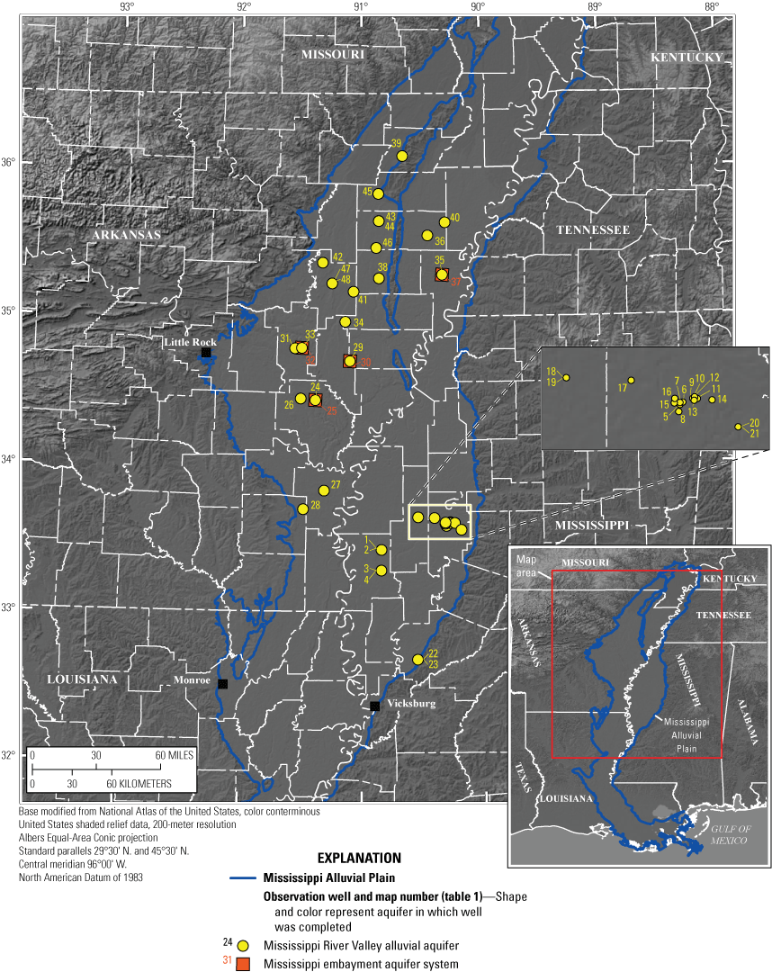
Locations of observation wells selected for slug testing in the Mississippi Alluvial Plain, Arkansas and Mississippi, 2020.
Table 1.
Location information for observation wells selected for slug testing in the Mississippi Alluvial Plain, Arkansas and Mississippi, 2020.[USGS, U.S. Geological Survey; Miss., Mississippi; Ark., Arkansas]
| Map number (fig. 1) | Site name for this study | Agency code | Site number (USGS, 2020) |
Latitude, in decimal degrees | Longitude, in decimal degrees | State | County |
|---|---|---|---|---|---|---|---|
| 1 | MS_BP-03a | USGS | 332514090500901 | 33.4206 | −90.8357 | Miss. | Washington |
| 2 | MS_BP-03b | USGS | 332514090500902 | 33.4206 | −90.8357 | Miss. | Washington |
| 3 | MS_BP-04a | USGS | 331654090501401 | 33.2816 | −90.8372 | Miss. | Washington |
| 4 | MS_BP-04b | USGS | 331654090501402 | 33.2816 | −90.8372 | Miss. | Washington |
| 5 | MS_OW-01 | USGS | 333535090180301 | 33.5931 | −90.3010 | Miss. | Leflore |
| 6 | MS_OW-02 | USGS | 333550090174201 | 33.5972 | −90.2950 | Miss. | Leflore |
| 7 | MS-OW-03 | USGS | 333547090180301 | 33.5965 | −90.3010 | Miss. | Leflore |
| 8 | MS-OW-04 | USGS | 333452090181301 | 33.5811 | −90.3036 | Miss. | Leflore |
| 9 | MS_OW-05 | USGS | 333613090162801 | 33.6035 | −90.2744 | Miss. | Leflore |
| 10 | MS_OW-06 | USGS | 333611090161501 | 33.603 | −90.2708 | Miss. | Leflore |
| 11 | MS_OW-08 | USGS | 333611090155401 | 33.603 | −90.2651 | Miss. | Leflore |
| 12 | MS_OW-09 | USGS | 333621090161401 | 33.6059 | −90.2707 | Miss. | Leflore |
| 13 | MS_OW-10 | USGS | 333600090161701 | 33.6001 | −90.2715 | Miss. | Leflore |
| 14 | MS_OW-12 | USGS | 333602090140501 | 33.6005 | −90.2346 | Miss. | Leflore |
| 15 | MS_OW-13 | USGS | 333545090184601 | 33.5959 | −90.3127 | Miss. | Leflore |
| 16 | MS_OW-14 | USGS | 333631090182501 | 33.6087 | −90.3068 | Miss. | Leflore |
| 17 | MS_QV-01a | USGS | 333805090240501 | 33.6348 | −90.4013 | Miss. | Leflore |
| 18 | MS_SF-02a | USGS | 333824090320701 | 33.6399 | −90.5353 | Miss. | Sunflower |
| 19 | MS_SF-02b | USGS | 333824090320702 | 33.64 | −90.5354 | Miss. | Sunflower |
| 20 | MS_YB-06a | USGS | 333315090105301 | 33.5542 | −90.1813 | Miss. | Leflore |
| 21 | MS_YB-06b | USGS | 333315090105302 | 33.5542 | −90.1813 | Miss. | Leflore |
| 22 | MS_YZ-07a | USGS | 324044090323401 | 32.6789 | −90.5429 | Miss. | Yazoo |
| 23 | MS_YZ-07b | USGS | 324044090323402 | 32.6789 | −90.5429 | Miss. | Yazoo |
| 24 | AR_ANRC_027N | AR008 | 342553091225101 | 34.4314 | −91.3808 | Ark. | Arkansas |
| 26 | AR_ANRC_028 | AR008 | 342630091300701 | 34.4417 | −91.5019 | Ark. | Arkansas |
| 27 | AR_ANRC_029 | AR008 | 334916091182501 | 33.8211 | −91.3069 | Ark. | Desha |
| 28 | AR_ANRC_030 | AR008 | 334144091284201 | 33.6956 | −91.4783 | Ark. | Drew |
| 29 | AR_ANRC_037N | AR008 | 344139091054201 | 34.6942 | −91.0950 | Ark. | Monroe |
| 31 | AR_ANRC_039 | AR008 | 344649091330001 | 34.7803 | −91.5500 | Ark. | Prairie |
| 33 | AR_ANRC_041S | AR008 | 344659091293701 | 34.7831 | −91.4936 | Ark. | Prairie |
| 34 | AR_ANRC_042 | AR008 | 345735091080101 | 34.9597 | −91.1336 | Ark. | St. Francis |
| 35 | AR_ANRC_001 | AR008 | 351630090193301 | 35.275 | −90.3258 | Ark. | Crittenden |
| 36 | AR_ANRC_003 | AR008 | 353224090264601 | 35.54 | −90.4461 | Ark. | Poinsett |
| 38 | AR_ANRC_007 | AR008 | 351508090511301 | 35.2522 | −90.8536 | Ark. | Cross |
| 39 | AR_ANRC_009 | AR008 | 360431090391701 | 36.0753 | −90.6547 | Ark. | Greene |
| 40 | AR_ANRC_014 | AR008 | 353740090180201 | 35.6278 | −90.3006 | Ark. | Poinsett |
| 41 | AR_ANRC_016 | AR008 | 350944091035401 | 35.1622 | −91.0650 | Ark. | Woodruff |
| 42 | AR_ANRC_017 | AR008 | 352128091191901 | 35.3578 | −91.3219 | Ark. | Woodruff |
| 43 | AR_USDA_1N | USDA | 353819090511201 | 35.6381 | −90.8536 | Ark. | Poinsett |
| 44 | AR_USDA_1S | USDA | 353816090511301 | 35.638 | −90.8536 | Ark. | Poinsett |
| 45 | AR_USGS_001 | USGS | 354916090512501 | 35.821 | −90.8568 | Ark. | Craighead |
| 46 | AR_USGS_002 | USGS | 352726090523101 | 35.4572 | −90.8754 | Ark. | Poinsett |
| 47 | AR_USGS_CR-03a | USGS | 351305091143401 | 35.2181 | −91.2427 | Ark. | Woodruff |
| 48 | AR_USGS_CR-03b | USGS | 351305091143402 | 35.2181 | −91.2427 | Ark. | Woodruff |
| 25 | AR_ANRC_027S | AR008 | 342553091225102 | 34.4314 | −91.3808 | Ark. | Arkansas |
| 30 | AR_ANRC_037S | AR008 | 344139091054202 | 34.6942 | −91.0950 | Ark. | Monroe |
| 32 | AR_ANRC_041N | AR008 | 344659091293702 | 34.7831 | −91.4936 | Ark. | Prairie |
| 37 | AR_ANRC_006 | AR008 | 351630090193302 | 35.275 | −90.3258 | Ark. | Crittenden |
The purpose of this report is to document the hydrogeologic setting, well descriptions, slug-testing and data analysis methods, and hydraulic conductivity and transmissivity estimates from slug tests conducted at 48 observation wells within the Mississippi Alluvial Plain of Arkansas and Mississippi. This report provides hydrogeologic information that hydrologists, groundwater modelers, and economists can use for water-availability planning and modeling. This work supports a major goal of the USGS Water Mission Area Science Strategy (Evenson and others, 2013) to “advance understanding of processes that determine water availability.” The data collection and analyses conducted as part of this study add to the understanding of the hydrogeology of the aquifers within the Mississippi embayment aquifer system and will aid in evaluating the occurrence, availability, and quality of groundwater to help support local water management.
These tests were conducted as part of the USGS Mississippi Alluvial Plain (MAP) Regional Water Availability Study, which is supported by the USGS Water Availability and Use Science Program. For the MAP Study, the USGS has partnered with the Arkansas Department of Agriculture Natural Resources Division, Arkansas Department of Health, Louisiana Department of Transportation and Development, Mississippi Delta Council, Delta F.A.R.M., Delta Wildlife, Mississippi Department of Environmental Quality, Yazoo Mississippi Delta Joint Water Management District, Missouri Department of Natural Resources, U.S. Army Corps of Engineers, and U.S. Department of Agriculture – Agricultural Research Service. The shared goal is to provide stakeholders and managers information and tools to better understand and manage groundwater resources within the MAP by using advanced characterization of the MAP, synthesis of field data, and numerical modeling.
Hydrogeologic Setting
The Mississippi River Valley alluvial aquifer underlies the Mississippi Alluvial Plain (table 2; figs. 1 and 2) and extends southward from the head of the Mississippi embayment aquifer system to where it merges with the Coastal Lowlands aquifer system near the Gulf of Mexico (Renken, 1998). The aquifer ranges from about 120 miles wide near the latitude of Little Rock, Arkansas, to 75 miles wide between Vicksburg, Mississippi, and Monroe, Louisiana. The aquifer consists of a braided, upward-fining sequence of gravel and coarse sand overlain by finer sand, silt, and clay that form a confining unit in most areas (Renken, 1998). The thickness of the Mississippi River Valley alluvial aquifer ranges from about 25 to about 200 feet (ft), and the thickness of the confining unit averages between 20 and 30 ft. The Mississippi River Valley alluvial aquifer directly overlies and in places is hydraulically interconnected with the deeper aquifers of the Mississippi embayment aquifer system (fig. 2) (Renken, 1998).
Table 2.
Hydrogeologic information for and descriptions of selected aquifers with wells that were slug tested in 2020 in the Mississippi Alluvial Plain. (Modified from Petersen and others [1985] and Renken [1998]).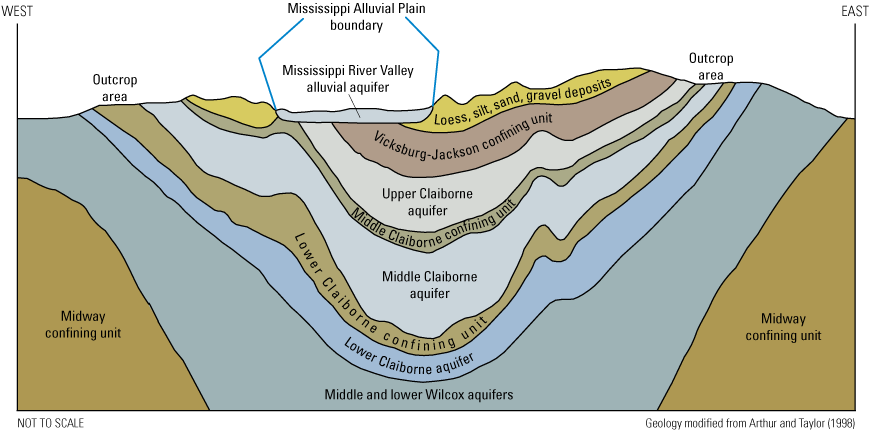
Generalized west-to-east profile of the Mississippi embayment aquifer system (modified from Arthur and Taylor, 1998).
The Mississippi embayment aquifer system extends eastward from Arkansas to northwestern Mississippi. The system consists of six aquifers of poorly consolidated to unconsolidated bedded sand, silt, and clay that have formed along the axis of the southerly plunging trough of the Mississippi embayment (fig. 2) (Renken, 1998).
Within the Mississippi embayment aquifer system, the middle Claiborne aquifer may be known locally as the Sparta and the Memphis aquifer (Hart and others, 2008) (table 2; fig. 2). The middle Claiborne aquifer is thickest in a large area of east-central Louisiana and southwestern Mississippi and in a smaller area of southeastern Arkansas, where the thickness is more than 1,000 ft and dissolved solids concentrations are greater than 1,000 milligrams per liter (Renken, 1998). In most areas where water in the middle Claiborne aquifer contains smaller concentrations of dissolved solids, the thickness of the aquifer generally ranges from 200 to 800 ft (Renken, 1998).
In most of its southern extent, confining units separate the middle Claiborne aquifer from underlying and overlying aquifers (fig. 2). The lower Claiborne confining unit underlies the middle Claiborne aquifer, and the middle Claiborne confining unit overlies the aquifer. Silt and clays that make up these confining units were deposited during widespread marine transgression periods that interrupted progradation of clastic sediments into the Gulf Coast Basin (Renken, 1998). Grain size in the lower Claiborne confining unit coarsens north of lat 35° N. and transitions to sandy channel sediments deposited in a coastal margin delta system (Hosman and others, 1968). In Arkansas and northernmost Mississippi, where the lower Claiborne confining unit is missing, the middle Claiborne aquifer and the lower Claiborne-upper Wilcox aquifers function as a single aquifer, which is known locally as the Memphis aquifer (Renken, 1998).
Well Descriptions
Slug tests were conducted on 48 observations wells located within the MAP in Arkansas and Mississippi during the spring and summer of 2020. The selection of test locations was based on information needs of the USGS MAP Regional Water Availability Study and other local, State, and Federal partners. Well-construction information was obtained from drillers’ construction reports on file with the Arkansas Natural Resources Commission, formerly the Arkansas Water Well Construction Commission (Arkansas Department of Agriculture, 2024) or the USGS National Water Information System database (USGS, 2020). Twenty-five of the tested observation wells are in Arkansas, and 23 are in Mississippi (fig. 1; table 1). Well-construction information required for hydraulic conductivity estimations includes the hole depth and diameter; the well depth and diameter; and the well opening (screen) top depth, length, and diameter (table 3).
Table 3.
Construction information for selected observation wells selected for slug testing in the Mississippi Alluvial Plain, Arkansas and Mississippi, 2020. Data from Pugh (2023).[ft, foot; bls, below land surface; in., inch; Open, well opening or screen]
Downhole Equipment—Transducers and Slugs
Downhole equipment dimensions for the pressure transducers and mechanical slugs are required to estimate hydraulic conductivity. Vented Level TROLL 700 Data Logger (In-Situ, Fort Collins, Colorado) pressure transducers were used to measure changes in the well water column during slug testing. The pressure transducers have an outside diameter of 0.72 inch (in.).
Twelve mechanical polyvinyl chloride slugs of various sizes and volumes were constructed and calibrated for this study (fig. 3). The slugs were constructed of capped, schedule-40 polyvinyl chloride pipes that were filled with gravel, and a steel eye bolt was installed in one end cap of each slug. The slugs were calibrated by repeatedly submerging them in a calibration well with a known diameter. Water levels were measured by using a calibrated electric water-level tape, and the volume of water displaced was calculated. Detailed slug dimensions and calibration information are available in the associated data release (Pugh, 2023).
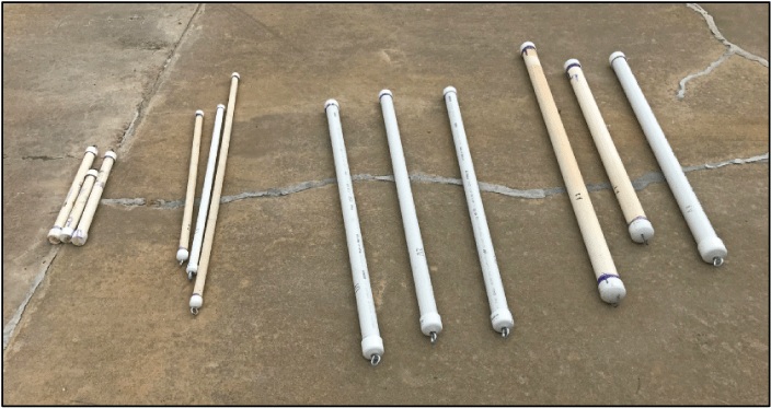
Mechanical slugs used during tests in selected wells to estimate hydraulic conductivity and transmissivity of aquifers in the Mississippi Alluvial Plain, Arkansas and Mississippi, 2020. Photograph by Aaron Pugh, U.S. Geological Survey, March 16, 2020.
Field Methods
Groundwater-Level Data Collection
Before and after each slug test, the static water level in each well was measured with a calibrated tape following the procedures specified in the USGS groundwater technical procedures document 1 in Cunningham and Schalk (2011). All static water-level measurements are available in the USGS National Water Information System database (USGS, 2020). The static water-level measurement at each well was used to help determine the aquifer’s saturated thickness. Additionally, the static water-level measurement was used to determine the depth to suspend the transducer below the water surface before slug testing and the depth to lower and raise the slug to ensure it was fully submerged during slug-in testing and completely above the water surface during slug-out testing.
Slug-Test Methods
The methods followed for the slug tests are presented in the USGS groundwater technical procedures document 17 in Cunningham and Schalk (2011). A minimum of 3 slug-in tests and 3 slug-out tests were conducted in 47 of the 48 wells tested. At well AR_ANRC_037S, completed in the Sparta aquifer, only two slug tests (two slug-in and two slug-out) were conducted because of excessively long water-level recovery times.
Slug testing began with an initial static water-level measurement followed by the deployment of the pressure transducer below the top of the water column in the well. The pressure transducer was connected to a laptop computer, set to record at a 0.25-second sampling interval, and the logging of water-level measurements was started. Once the water level in the well returned to the static level following transducer deployment, the first slug-in test was initiated by quickly lowering a mechanical slug completely below the water surface which caused the water level in the well to rise (fig. 4A and 4B). Once the water level returned to the static level, the slug-in test was considered complete. The second test, a slug-out test, was then initiated by quickly pulling the mechanical slug up so it was completely above the water surface, thus causing the water level to fall (fig. 4C and 4D). Once the water level returned to the static level, the slug-out test was considered complete. This process was repeated twice more, providing six different slug tests, three slug-in tests and three slug-out tests, for the well. When the six slug tests were complete, the data logging was stopped, and the data-log file was up-loaded to the laptop. The pressure transducer was then removed from the well, and a second static water-level measurement was made.
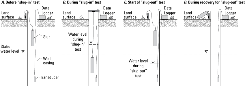
Well diagrams showing a mechanical slug and pressure transducer: A, mechanical slug poised just above the water level before slug-in test, B, mechanical slug submerged below water level for slug-in test, C, mechanical slug removed just above water level for slug-out test, and D, mechanical slug removed from well following slug-out test (from Cunningham and Schalk, 2011).
During testing, water levels were considered static when they equaled the initial static water-level measurement or when the change in water level was less than 0.01 ft per 10 minutes. For slug testing, the data collected during the beginning of the test are usually the most important for the water-level curve matching used to estimate hydraulic conductivity values (Cunningham and Schalk, 2011). When water-level changes were less than 0.01 ft per 10 minutes during the latter part of the test, the tests were considered to provide good-quality data for estimating hydraulic conductivity values. For most of the tests, water levels returned to a pre-testing static condition in less than 5 minutes following the insertion or removal of the mechanical slug, although this took considerably longer for a few tests.
Photographic Documentation
Photographs were taken at well sites for basic documentation (fig. 5). Images are available, by well site, in Pugh (2023).
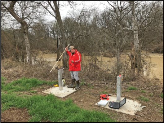
U.S. Geological Survey employee preparing to insert a mechanical slug into the well being tested at well MS_QV-01a in Mississippi, March 17, 2020. (Photograph by Aaron Pugh, U.S. Geological Survey.)
Analytical Methods for Estimating Hydraulic Conductivity
Water-level changes for each slug test were analyzed by using one of three slug-test methods based on the well and aquifer information and by using aquifer test analysis software, AQTESOLV version 4.50.002 (HydroSOLVE, Inc., 2007). The Bouwer and Rice (1976) solution was used on overdamped slug-test responses in full or partially penetrating wells in confined and unconfined aquifers. The response data from an overdamped slug test are generally decreasing monotonically with increasing time (log head or normalized head versus time) and occur in aquifers with low to moderate hydraulic conductivity values (HydroSOLVE, Inc., 2007). The Springer and Gelhar (1991) and Butler (1998) methods were used on underdamped slug-test responses. The response data during an underdamped slug test are oscillatory with increasing time and occur in aquifers with high hydraulic conductivity values (HydroSOLVE, Inc., 2007).
The aquifer test analysis software provides two estimates for each slug-test estimate of hydraulic conductivity. The first estimate is an “automatic estimate” using an automatic curve-fitting algorithm to create a best-fit curve by varying the effective well length and the hydraulic conductivity parameters until the curve best fits the observed water-level data. The effective well length equals the height of the water column above the top of the screen plus one-half the screen length. The second estimate is a “visual estimate” using a user-generated best-fit curve match of the water-level data made by manually varying the effective well length and the hydraulic conductivity parameters.
Both the visual and automatic curve-fitting estimates were recorded and used to develop the statistical summary of estimates for each well. All visual curve-fitting estimates were used; however, a few automatic curve-fitting estimates were discarded because of spurious water-level measurements resulting in excessively large estimates when compared to the other test estimates for the same well. These spurious water-level measurements may have occurred when splashing and sloshing water was recorded by the pressure transducer. The analyzed results for the slug tests conducted in each well are available from Pugh (2023).
Analytical Methods for Estimating Transmissivity
Estimates of transmissivity were made by multiplying the estimated hydraulic conductivity value by the aquifer thickness at the well location. Aquifer thicknesses were obtained from Torak and Painter (2019) or the interactive Mississippi Embayment Regional Aquifer (MERAS) Hydrogeologic Framework web application (USGS, undated).
Limitations and Assumptions
The hydraulic conductivity estimated by a slug test represents a small volume of the aquifer material surrounding the tested well, not the average hydraulic conductivity of the aquifer. Hydraulic conductivity estimates from slug tests are usually smaller than those estimated from pumping tests (Brown and others, 1995). Hydraulic conductivity estimates from slug tests are influenced by the well filter packs, wellbore skin effects, and solution method assumptions made during analysis.
Well filter packs will influence the estimated hydraulic conductivity if they have a different hydraulic conductivity than the surrounding, undisturbed aquifer formation. A filter pack is the coarse sand or fine gravel placed between the borehole wall and screen that filters fine-grained particles, preventing them from entering the well (Butler, 1998).
Similarly, a wellbore skin will influence the estimated hydraulic conductivity because it is a zone of differing hydraulic conductivity adjacent to the wellbore face resulting from well construction and (or) development (Butler, 1998). A positive wellbore skin is a zone adjacent to the wellbore with a smaller hydraulic conductivity than that of the undisturbed aquifer formation. A positive wellbore skin may occur if, during construction, bentonite drilling mud is used or fine-grained formation materials are smeared across the wellbore face of larger grained materials, and the well is not properly completed. A negative wellbore skin is a zone with a hydraulic conductivity larger than that of the undisturbed aquifer formation. A negative wellbore skin may occur when finer grained particles at the wellbore face are eroded away and can occur with excessive well development (Butler, 1998).
Bouwer and Rice Method
The Bouwer and Rice (1976) method is a semi-analytical method for the analysis of overdamped slug tests in a fully or partially penetrating well in an unconfined or confined aquifer. The Bouwer and Rice method employs a quasi-steady-state model that ignores elastic storage in the aquifer (HydroSOLVE, Inc., 2007). The Bouwer and Rice method makes the following assumptions: (1) the aquifer has infinite areal extent, (2) the aquifer is homogeneous and of uniform thickness, (3) the test well is fully or partially penetrating, (4) the aquifer is confined or unconfined, (5) flow to the well is quasi-steady state (storage is negligible), and (6) the slug is introduced into or removed from the well instantaneously.
Springer and Gelhar Method
The Springer and Gelhar (1991) method extended the Bouwer and Rice (1976) method for a slug test in a homogeneous, anisotropic, unconfined aquifer to include inertial effects in the test well. The solution accounts for oscillatory water-level response sometimes observed in aquifers with high hydraulic conductivity. Based on the work of Butler (2005), AQTESOLV has incorporated frictional well loss in small-diameter wells (HydroSOLVE, Inc., 2007). The Springer and Gelhar method makes the following assumptions: (1) the aquifer has infinite areal extent, (2) the aquifer is homogeneous and of uniform thickness, (3) the test well is fully or partially penetrating, (4) the aquifer is unconfined, (5) the flow is quasi-steady state, and (6) the slug is introduced into or removed from the well instantaneously.
Butler Method
The Butler (1998) method extended the Hvorslev (1951) solution for a single-well slug test in a homogeneous, anisotropic, confined aquifer to include inertial effects in the test well. The solution accounts for oscillatory water-level response sometimes observed in aquifers with high hydraulic conductivity. Butler (2005) amended the method to incorporate frictional well loss in small-diameter wells. The Butler method makes the following assumptions: (1) the aquifer has infinite areal extent, (2) the aquifer is homogeneous and of uniform thickness, (3) test well is partially penetrating, (4) the aquifer is confined, (5) the flow is quasi-steady state, and (6) the slug is introduced into or removed from the well instantaneously.
Hydraulic Conductivity and Transmissivity Estimates
A total of 324 slug tests were conducted, providing 598 estimates of hydraulic conductivity and transmissivity. Based on the methodology described earlier, only 576 slug-test estimates would be expected (48 tested wells × 6 tests/well × 2 estimates/test). Additional slug tests were conducted for the following reasons: (1) during training, two sets of three slug tests (three slug-in tests and three slug-out tests) were conducted on well MS_OW-05 by different USGS personnel, and (2) USGS personnel conducted additional sets of slug tests (a slug-in test and a slug-out test) whenever there were questions or problems with a previous set of slug tests. Wells where additional sets of tests were conducted have more than 12 test estimates (tables 4 and 5).
Table 4.
Estimated hydraulic conductivity for aquifers at selected wells in the Mississippi Alluvial Plain, Arkansas and Mississippi, 2020. Data from Pugh (2023).[ft, foot; dates are in month/day/year format; bls, below land surface; ft/d, foot per day; n, number of test estimates; Min, minimum, Max, maximum; Springer-Gelhar (Springer and Gelhar, 1991); Bouwer-Rice (Bouwer and Rice, 1976); Butler (Butler, 1998)]
Table 5.
Estimated transmissivity for aquifers at selected wells in the Mississippi Alluvial Plain, Arkansas and Mississippi, 2020. Data from Pugh (2023).[ft, foot; dates are in month/day/year format; bls, below land surface; ft2/d, foot squared per day; n, number of test estimates; Min, minimum, Max, maximum; Springer-Gelhar (Springer and Gelhar, 1991); Bouwer-Rice (Bouwer and Rice, 1976); Butler (Butler, 1998)]
Unusable or questionable test data occurred with one or more tests from 11 wells. Data were unusable or questionable because (1) the selection of a slug was too small, resulting in logging abnormalities; (2) recovery times were excessively long when compared to other slug tests conducted in the same well; (3) data-log files were empty; or (4) excessively large automatic estimates were 2 to 3 orders of magnitude larger than the other test estimates from the same well. Unusable or questionable data were not used for final estimates. Wells where unusable or questionable test data occurred will have fewer than 12 test estimates (tables 4 and 5).
Estimates of hydraulic conductivity and transmissivity for the Mississippi River Valley alluvial aquifer were calculated for 44 wells from 555 slug tests (tables 4 and 5). Mean hydraulic conductivity estimates range from 3 to 401 feet per day (ft/d), and median hydraulic conductivity estimates range from 3 to 381 ft/d. Mean transmissivity estimates for these wells range from 285 to 80,559 feet squared per day (ft2/d), and median transmissivity estimates range from 293 to 76,449 ft2/d.
Estimates of hydraulic conductivity and transmissivity for the middle Claiborne aquifer were calculated for 4 wells from 43 slug tests (tables 4 and 5). Mean hydraulic conductivity estimates range from 0.14 to 183 ft/d, and median hydraulic conductivity estimates range from 0.15 to 103 ft/d. Mean transmissivity estimates range from 55 to 67,913 ft2/d, and median transmissivity estimates range from 59 to 38,416 ft2/d.
Summary
Single-well slug tests were conducted by the U.S. Geological Survey during the spring and summer of 2020 at 48 wells to estimate the hydraulic conductivity and transmissivity at selected well sites within the Mississippi Alluvial Plain in Arkansas and Mississippi. Data collection included well and aquifer data from the field and well-construction information from drillers’ construction reports. Multiple slug-in and slug-out tests were completed at each well by using a mechanical slug following published U.S. Geological Survey methods and standards. A total of 324 slug tests were conducted. Aquifer hydraulic conductivity was estimated by curve fitting the observed water-level-change data using aquifer test analysis software. Estimates of aquifer transmissivity were made by multiplying the estimated hydraulic conductivity by the aquifer thickness at each well location. Mean hydraulic conductivity estimates for 44 wells screened in the Mississippi River Valley alluvial aquifer range from 3 to 401 feet per day, and mean transmissivity estimates range from 285 to 80,559 feet squared per day. Mean hydraulic conductivity estimates for 4 wells screened in units of the middle Claiborne aquifer range from 0.14 to 183 feet per day, and mean transmissivity estimates range from 55 to 67,913 feet squared per day. The results from these tests can be used to improve our understanding of water availability and to refine groundwater models, and the results provide stakeholders and groundwater resource managers information about the groundwater resources within the Mississippi Alluvial Plain.
References Cited
Arkansas Department of Agriculture, 2024, Water well construction: Arkansas Department of Agriculture webpage, accessed August 21, 2024, at https://agriculture.arkansas.gov/arkansas-water-well-construction/the-commission/.
Arthur, J.K., and Taylor, R.E., 1998, Ground-water flow analysis of the Mississippi embayment aquifer system, South-Central United States: U.S. Geological Survey Professional Paper 1416–1, 148 p., 9 pls. [Also available at https://pubs.er.usgs.gov/publication/pp1416I.]
Bouwer, H., and Rice, R.C., 1976, A slug test for determining hydraulic conductivity of unconfined aquifers with completely or partially penetrating wells: Water Resources Research, v. 12, no. 3, p. 423–428, accessed September 2020 at https://agupubs.onlinelibrary.wiley.com/doi/abs/10.1029/WR012i003p00423.
Brown, D.L., Narasimhan, T.N., and Demir, Z., 1995, An evaluation of the Bouwer and Rice method of slug test analysis: Water Resources Research, v. 31, no. 5, p. 1239–1246, accessed September 2020 at https://agupubs.onlinelibrary.wiley.com/doi/abs/10.1029/94WR03292.
Butler, J.J., Jr., 2005, A simple correction for slug tests in small-diameter wells: Groundwater, v. 40, no. 3, p. 303–308, accessed September 2020 at https://ngwa.onlinelibrary.wiley.com/doi/10.1111/j.1745-6584.2002.tb02658.x.
Cunningham, W.L., and Schalk, C.W., comps., 2011, Groundwater technical procedures of the U.S. Geological Survey: U.S. Geological Survey Techniques and Methods 1–A1, 151 p., accessed December 2019 at https://pubs.usgs.gov/tm/1a1/.
Evenson, E.J., Orndorff, R.C., Blome, C.D., Böhlke, J.K., Hershberger, P.K., Langenheim, V.E., McCabe, G.J., Morlock, S.E., Reeves, H.W., Verdin, J.P., Weyers, H.S., and Wood, T.M., 2013, U.S. Geological Survey Water Science Strategy—Observing, understanding, predicting, and delivering water science to the Nation: U.S. Geological Survey Circular 1383–G, 49 p., accessed December 2020 at https://doi.org/10.3133/cir1383G.
Hart, R.M., Clark, B.R., and Bolyard, S.E., 2008, Digital surfaces and thicknesses of selected hydrogeologic units within the Mississippi Embayment Regional Aquifer Study (MERAS): U.S. Geological Survey Scientific Investigations Report 2008–5098, 33 p. [Also available at https://pubs.usgs.gov/sir/2008/5098/.]
Hosman, R.L., Long, A.T., Lambert, T.W., and Jeffery, H.G., 1968, Tertiary aquifers in the Mississippi embayment, with discussions of quality of the water: U.S. Geological Survey Professional Paper 448–D, 29 p., accessed August 2020 at https://doi.org/10.3133/pp448D.
Hvorslev, M.J., 1951, Time lag and soil permeability in ground-water observations: Vicksburg, Miss., Waterways Experiment Station, U.S. Army Corps of Engineers, Bulletin No. 36, 50 p., accessed September 2020 at https://erdc-library.erdc.dren.mil/jspui/bitstream/11681/4796/1/BUL-36.pdf.
HydroSOLVE, Inc., 2007, AQTESOLV for Windows, user’s guide: Reston, Va., 529 p., accessed February 13, 2020, at http://www.aqtesolv.com/download/aqtw20070719.pdf.
Petersen, J.C., Broom, M.E., and Bush, W.V., 1985, Geohydrologic units of the Gulf Coastal Plain in Arkansas: U.S. Geological Survey Water-Resources Investigations Report 85–4116, 20 p., 9 pls. [Also available at https://pubs.er.usgs.gov/publication/wri854116.]
Pugh, A.L., 2023, Hydraulic conductivity and transmissivity estimates from slug tests in wells within the Mississippi Alluvial Plain, Arkansas and Mississippi, 2020: U.S. Geological Survey data release, https://doi.org/10.5066/P9AXRVT7.
Renken, R.A., 1998, Ground water atlas of the United States—Arkansas, Louisiana, Mississippi: U.S. Geological Survey Hydrologic Atlas HA 730–F, p. 65–83. [Also available at https://pubs.usgs.gov/ha/ha730/ch_f/F-text4.html.]
Springer, R.K., and Gelhar, L.W., 1991, Characterization of large-scale aquifer heterogeneity in glacial outwash by analysis of slug tests with oscillatory responses, Cape Cod, Massachusetts, in Mallard, G.E., and Aronson, D.A., eds., U.S. Geological Survey Toxic Substances Hydrology Program—Proceedings of the technical meeting, Monterey, California, March 11–15, 1991: U.S. Geological Survey Water-Resources Investigations Report 91–4034, p. 36–40, accessed September 2020 at https://pubs.er.usgs.gov/publication/wri914034.
Torak, L.J., and Painter, J.A., 2019, Geostatistical estimation of the bottom altitude and thickness of the Mississippi River Valley alluvial aquifer: U.S. Geological Survey Scientific Investigations Map 3426, 2 sheets, accessed August 2020 at https://doi.org/10.3133/sim3426.
U.S. Geological Survey [USGS], 2020, USGS water data for the Nation: U.S. Geological Survey National Water Information System database, accessed September 15, 2020, at https://doi.org/10.5066/F7P55KJN.
U.S. Geological Survey [USGS], [undated], MERAS Groundwater Availability Study, subsurface map, accessed July 1, 2020, at https://www2.usgs.gov/water/lowermississippigulf/lmgweb/meras/submap.html.
Conversion Factors
U.S. customary units to International System of Units
For more information about this publication, contact
Director, Lower Mississippi-Gulf Water Science Center
U.S. Geological Survey
640 Grassmere Park, Suite 100
Nashville, TN 37211
For additional information, visit
https://www.usgs.gov/centers/lmg-water/
Publishing support provided by
Lafayette Publishing Service Center
Disclaimers
Any use of trade, firm, or product names is for descriptive purposes only and does not imply endorsement by the U.S. Government.
Although this information product, for the most part, is in the public domain, it also may contain copyrighted materials as noted in the text. Permission to reproduce copyrighted items must be secured from the copyright owner.
Suggested Citation
Pugh, A.L., 2025, Hydraulic conductivity and transmissivity estimates from slug tests in wells within the Mississippi Alluvial Plain, Arkansas and Mississippi, 2020: U.S. Geological Survey Scientific Investigations Report 2023–5101, 17 p., https://doi.org/10.3133/sir20235101.
ISSN: 2328-0328 (online)
Study Area
| Publication type | Report |
|---|---|
| Publication Subtype | USGS Numbered Series |
| Title | Hydraulic conductivity and transmissivity estimates from slug tests in wells within the Mississippi Alluvial Plain, Arkansas and Mississippi, 2020 |
| Series title | Scientific Investigations Report |
| Series number | 2023-5101 |
| DOI | 10.3133/sir20235101 |
| Publication Date | July 02, 2025 |
| Year Published | 2025 |
| Language | English |
| Publisher | U.S. Geological Survey |
| Publisher location | Reston, VA |
| Contributing office(s) | Lower Mississippi-Gulf Water Science Center |
| Description | Report: iv, 17 p.; Data Release |
| Country | United States |
| State | Arkansas, Mississippi |
| Other Geospatial | Mississippi Alluvial Plain |
| Online Only (Y/N) | Y |