

Evaluation of Stream Capture Related to Groundwater Pumping, Lower Humboldt River Basin, Nevada
Links
- Document: Report (26 MB pdf) , HTML , XML
- Data Release: USGS Data Release - MODFLOW-NWT Model and Supplementary Data Used to Characterize Effects of Pumping in Lovelock Valley, Nevada
- NGMDB Index Page: National Geologic Map Database Index Page (html)
- Download citation as: RIS | Dublin Core
Acknowledgments
This study was supported by the Nevada Division of Water Resources. The authors would like to thank Bennie Hodges and the Pershing County Water Conservation District for familiarizing the authors with the study area and for providing valuable insight and resources related to Lovelock Valley. The authors also would like to thank C.J. Mayers of the U.S. Geological Survey for developing the Python scripts used in this study and for his insight in automating many of the calculations and routines. A great deal of thanks are due to Rose Medina of the U.S. Geological Survey for crafting many of the figures and for her assistance with all things having to do with the Geographic Information System (GIS). The authors also would like to thank Greg Pohll of the Truckee Meadows Water Authority and Kip Allander of the Nevada Division of Water Resources for their mentorship during this study. The authors would also like to thank Kyle Davis and Phil Gardner of the U.S. Geological Survey and Rosemary Carol of the Desert Research Institute for their valuable reviews. Finally, the authors owe a great deal of thanks to Kelley Sterle of Environmental Science Associates for her help with data analysis and flow budget assessment.
Abstract
The Humboldt River Basin is the only river basin that is contained entirely within the State of Nevada. The effect of groundwater pumping on the Humboldt River is not well understood. Tools are needed to determine stream capture and manage groundwater pumping in the Humboldt River Basin. The objective of this study is to estimate capture and storage change caused by groundwater withdrawals in the lower Humboldt River Basin that can provide the Nevada State Engineer with data and information needed to manage groundwater and surface-water resources.
A numerical groundwater flow model was developed for the purpose of estimating stream capture from pre-2016 and future pumping as well as for any location of potential future pumping within the lower Humboldt River Basin. This model was developed using MODFLOW-NWT to represent the lower Humboldt River Basin hydrologic system, including Humboldt River; Rye Patch Reservoir; groundwater evapotranspiration; pumping from municipal, agricultural, mining, and domestic wells; and agricultural drains. Aquifer properties were calibrated using results from numerous single- and multi-well aquifer tests (Nadler, 2020) and through the process of model calibration.
Historical capture was estimated for 1960–2016 and predictive capture for the system was projected 100 years into the future (2017–2116) based on historical pumping patterns. Stream capture and drain capture are relatively low for the historical and predictive periods. During the historical period, increased pumping during dry years caused increased connections with capture sources and less water sourced to wells from aquifer storage. Storage and groundwater levels generally recovered during subsequent wet years. Overall, storage change has been the main source of water to wells in the lower Humboldt River Basin, followed by groundwater evapotranspiration capture. During the predictive period, pumping is projected to remain constant and capture 9 percent of stream water after 100 years.
Capture and storage change maps were created to visualize spatial variability in potential capture and storage change through time and to provide a database of results that can be used to manage groundwater and surface-water resources. These maps show that potential stream capture would be a minor source of water to wells located across most of the simulated area, except for locations close to the Humboldt River and Rye Patch Reservoir. Drains also would be a minor potential source of water to wells except for those directly adjacent to the drains. In general, the potential supply of water to wells is storage-dominated and over time groundwater evapotranspiration-dominated in the agricultural area.
Capture difference maps were generated to visualize where potential capture results might have greater limitations associated with nonlinear flow processes, such as head-dependent boundary conditions. Higher capture differences indicate larger capture map bias and therefore greater capture map uncertainty due to the inability of capture maps to account for nonlinear flow processes. Stream capture differences are highest directly adjacent to the river but are otherwise minimal. Drain capture differences are highest in the region of the agricultural drain network but are otherwise minimal. The Humboldt River, Rye Patch Reservoir, and drains introduce very little nonlinearity to the model, and their associated capture map bias is minimal. Potential groundwater evapotranspiration capture introduces a fair amount of nonlinearity to the model and has the potential to result in significant, localized groundwater evapotranspiration capture map bias over time. Groundwater evapotranspiration capture differences are the result of higher pumping rates lowering the water table below the root zone faster than lower pumping rates and essentially removing groundwater evapotranspiration as a potential source of capture faster than lower pumping rates. Wells that can no longer source their supply through groundwater evapotranspiration capture then generally source more of their water from storage. Thus, storage change bias increases over time as well.
Capture prediction uncertainty due to parameter estimation was evaluated using a covariance matrix adaptation-evolution strategy. One hundred Monte Carlo realizations of model parameters were applied to the model to assess capture uncertainty at 13 grid cell locations within the model domain. In general, results indicated that greater capture uncertainty for a given source (river, drains, or evapotranspiration) is associated with proximity of a pumping well to that source. The magnitude of maximum capture fraction uncertainties after 100 years of pumping for stream capture, drain capture, groundwater evapotranspiration capture, and storage change were plus or minus (±) 0.17, ±0.10, ±0.20, and ±0.22, respectively.
Introduction
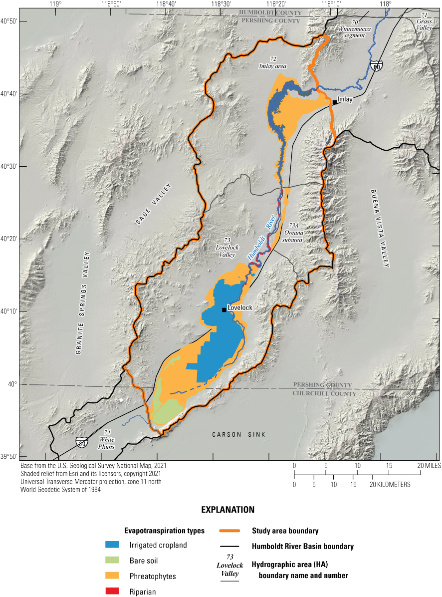
The Humboldt River Basin (HRB; fig . 1), in north-central Nevada, is the only major river basin entirely within the State of Nevada. The Humboldt River corridor is approximately 300 miles (mi) in length between the start and terminus, though the channel is significantly longer due to the river’s notable sinuosity. Previous work has demonstrated that the river’s surface-water resource is sensitive to groundwater withdrawals, which have steadily increased since the 1950s for agriculture, municipal, and mining uses (Prudic, 2007).
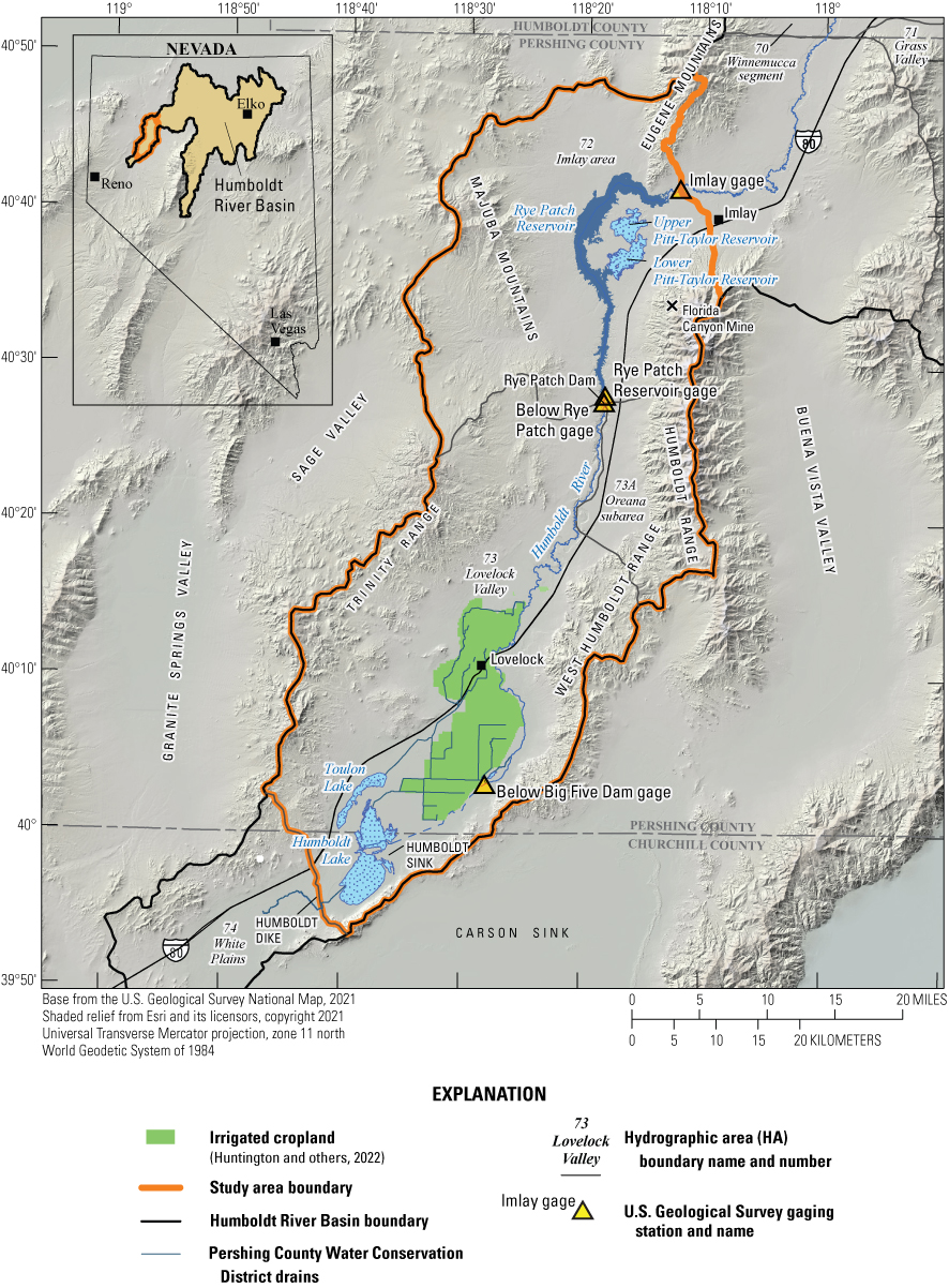
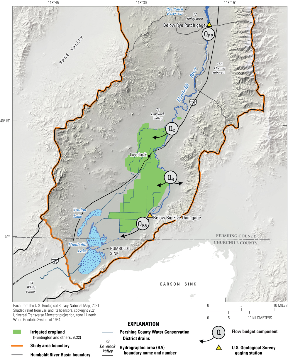
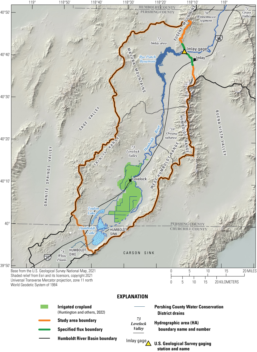
Location and major hydrologic features of Humboldt River Basin within the lower Humboldt River Basin study area.
Nevada water law follows the doctrine of prior appropriation, a “first in time, first in right” approach that prioritizes senior water rights (Welden, 2003; State of Nevada Division of Water Resources, 202140). Additionally, Nevada has historically administered surface water and groundwater separately. Because these two systems are often hydraulically connected, groundwater pumping may deplete, or capture, surface-water sources such as streams, springs, and lakes (Barlow and Leake, 2012), leading to conflict between surface-water and groundwater right holders.
Purpose and Scope
The effect of groundwater withdrawal on the Humboldt River is not well understood. The Desert Research Institute (DRI) and the U.S. Geological Survey (USGS) Nevada Water Science Center have concurrently developed three numerical groundwater flow models of the upper, middle, and lower HRB to quantify potential stream capture caused by groundwater withdrawals.
The objective of the study presented in this report is to estimate Humboldt stream capture caused by groundwater withdrawals within the lower HRB occurring downstream of Imlay to the Humboldt Dike (fig. 1), which falls on the boundary between the Lovelock Valley and White Plains hydrographic areas, for up to 100 years of groundwater withdrawals. The estimates were derived from a numerical groundwater flow model and displayed using stream capture maps.
The stream capture maps will provide the Nevada State Engineer and Nevada Division of Water Resources with appropriate information to understand and evaluate the historical and potential future effects of groundwater withdrawals on Humboldt River capture. Furthermore, stream capture maps can be used to assist in decisions related to managing the effects of groundwater pumping on surface water availability. Finally, this work will provide the State of Nevada with tools to inform stakeholders within the HRB about processes related to the interaction between groundwater and surface water.
Description of the Lower Humboldt River Basin
The HRB is within the Basin and Range province and is topographically characterized by north-south trending mountains surrounding flat valleys (Bredehoeft, 1963). The lower HRB, as defined in this study, is 1,160 square miles and is bounded by the Trinity Range to the west and the Humboldt Range to the east (fig. 1; Robinson and Fredericks, 1946). The Trinity Range has a maximum elevation of 7,332 feet (ft) and is on average 3,000 ft above the valley floor (Robinson and Fredericks, 1946). The Humboldt Range has a maximum elevation of about 9,000 ft, which is approximately 4,500 ft above the valley floor (Robinson and Fredericks, 1946). Lovelock Valley generally slopes downward from north to south with elevations ranging between 4,300 ft in the northern extent and 3,900 ft in the southern extent (Robinson and Fredericks, 1946). Accordingly, the Humboldt River flows from north to south, where it drains to the Humboldt Sink (fig. 1; Robinson and Fredericks, 1946; Bredehoeft, 19634).
The study area is contained within Pershing and Churchill Counties. Pershing County contains most of the Humboldt River in the lower HRB and Churchill County contains most of the Humboldt Sink (fig. 1). Interstate 80 runs generally north-south through the study area. The City of Lovelock is in the south-central region of the study area and is home to about 2,400 residents (cityoflovelock.com), and contains over 40,000 acres of the Lovelock Valley agricultural lands. The Lovelock Valley agricultural lands primarily produce alfalfa, wheat, hay, oats, and barley (Breazeale and Owens, 2000).
The lower HRB includes the southwestern section of hydrographic area (HA) 72 (Imlay area) and the entirety of HAs 73 and 73A (Lovelock Valley and the Oreana subarea), encompassing the stretch of the Humboldt River between the Imlay gage and the Humboldt Dike, and includes the Humboldt Sink (fig. 1). The Humboldt Sink occasionally fills to become an ephemeral lake but is typically dry most years. Lovelock Valley is approximately 65-mi long and varies in width between 6 mi in the northern part of the valley and 12 mi in the area surrounding the City of Lovelock (Robinson and Fredericks, 1946).
Rye Patch Reservoir, a 22-mi-long reservoir that stores and provides water to Lovelock irrigators, is in the northern part of the lower HRB. Rye Patch Reservoir and Dam were constructed by the Bureau of Reclamation between 1935 and 1936 (Eakin, 1962; Eakin and Lamke, 1966; Prudic and others, 2006). Rye Patch Dam is approximately 24 mi north of the City of Lovelock (Eakin, 1962). Water stored in the reservoir is typically released during irrigation season (March 15 through October 15) and in high-flow years when at near-capacity or for flood control. The maximum storage capacity of Rye Patch Reservoir is approximately 194,300 acre-feet per year (acre-ft/yr; Prudic and others, 2006). Streamflow is primarily derived from the high mountains in the upper HRB. No major tributaries contribute to the Humboldt River within the lower HRB.
There are three stream gages (hereinafter referred to as gages) within the study area (fig. 2) and one reservoir storage gage within the Rye Patch Reservoir. The full USGS gage names and their local names (used for the remainder of this report) are shown in table 1. The Imlay gage is of particular importance because it is located at the upstream boundary of the study area and has a streamflow record dating back to the 1930s.
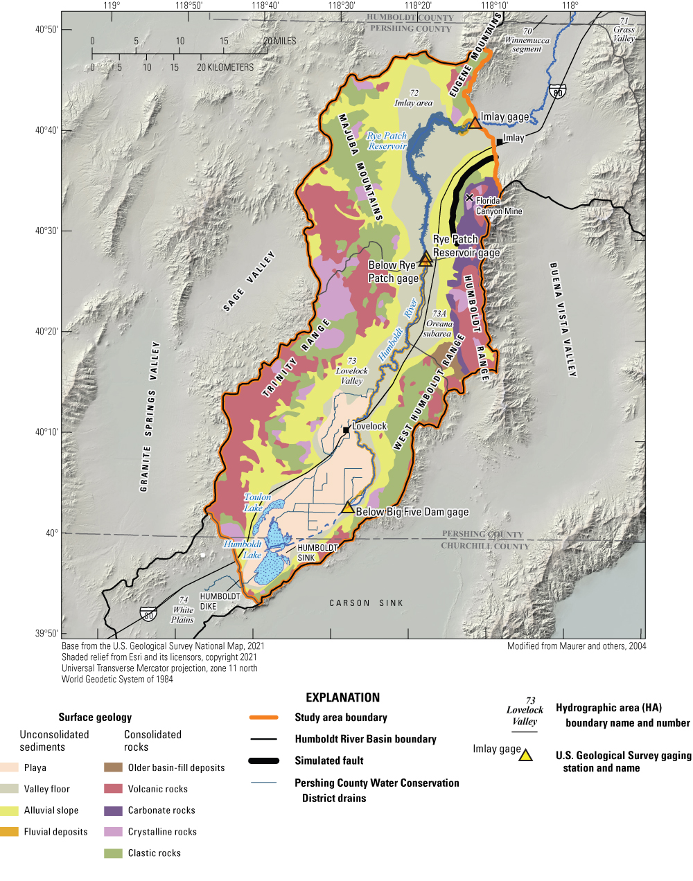
Surface geology within the lower Humboldt River Basin study area. Pershing County Water Conservation District drains are shown in blue. Fluvial deposits do not extend far from the Humboldt River and are therefore difficult to visualize on this map.
Table 1.
Gage names used within this report in reference to U.S. Geological Survey (USGS) stream gages within the lower Humboldt River Basin study area.[RV, river; NR, near; NV, Nevada; RES, reservoir]
The City of Lovelock, Nevada, is home to an agricultural community, and many acres within and near the city are used to grow alfalfa and other crops. In average and wet water years, farmers primarily irrigate with water diverted from the Humboldt River. Supplemental wells are used during dry years when the stage in Rye Patch Reservoir is too low to release additional streamflow for agriculture (Everett and Rush, 1965). The Lovelock area water budget is dominated by evapotranspiration (ET) from the fields (Everett and Rush, 1965).
Hydrogeologic Units of the Lower Humboldt River Basin
Lovelock Valley is characterized by three primary hydrogeologic units: (1) consolidated rock (late Paleozoic to Cenozoic), (2) water-bearing older alluvium (late Tertiary and Quaternary), and (3) younger alluvium (Pleistocene; Everett and Rush, 1965). The low-permeability consolidated rock surrounds and underlies the valley. The older alluvium is unconsolidated to poorly consolidated and consists of gravel, sand, silt, and clay. The older alluvium lines the mountains and underlies the younger alluvium away from the mountain margins. The younger alluvium contains the primary water-bearing sediments in Lovelock Valley and is the main focus of this study (Everett and Rush, 1965). The younger alluvium is composed of gravel, sand, silt, and clay sourced as colluvium from the surrounding mountains; fluvial sediments of the meandering and braided Humboldt River paleochannel; and lacustrine sediments from Pleistocene Lake Lahontan. Lake Lahontan clays and silts constitute the upper part of the younger alluvium and are reported to blanket the basin with a thickness of 20–35 ft (Everett and Rush, 1965). Well logs in Lovelock Valley indicate this clay and silt may be 50 ft thick in places. A layer of coarser material in the younger alluvium that underlies the Lake Lahontan clay and silt layer comprises the primary aquifer (Everett and Rush, 1965) and has been shown to be at least 1,365 ft thick at the location of the deepest drilled well in the area, though most wells penetrated less than 400 ft of the younger alluvium.
Hydrogeologic units defined by Maurer and others (2004) include 12 units categorized by rock type and age for Lovelock Valley. Surface geologic units were combined based on rock type, removing the age component, which resulted in nine generalized units (fig. 2). These generalized geologic units served as the initial hydrogeologic zones used for model calibration, though they were ultimately simplified further as described later in this report.
Aquifer Properties
Multiple aquifer tests were conducted in Lovelock, Nevada, to determine aquifer properties to be used with the numerical groundwater flow model of the lower HRB (Nadler, 2020). Seven slug tests, one single-well pumping test, and two multi-well pumping tests were conducted to evaluate properties of shallow Lahontan clays and silts, shallow fluvial deposits, and coarser, water-bearing deposits of the younger alluvium. Aquifer tests were conducted between March 2017 and April 2018. Multi-well pumping test 1 was conducted in March 2017 for a duration of 4 days. Multi-well pumping test 2 was conducted in November and December of 2017 for a duration of 6 days. Results indicate that unconsolidated aquifers in the Lovelock Valley have transmissivity ranging between 0.0001 and 95,000 square feet per day (ft2/d; table 2; fig. 3; Nadler, 2020). The results of these tests provide initial constraints on hydraulic properties for the numerical groundwater flow model of the lower HRB.
Table 2.
Estimated transmissivities of selected groupings of hydrostratigraphic units around locations of pumping wells (Nadler, 2020).[ft2/d; square foot per day]
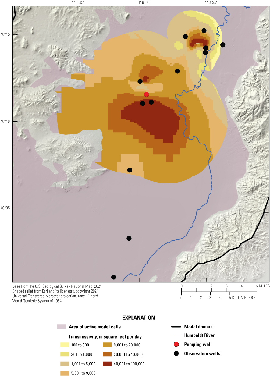
Estimated transmissivity of the area of drawdown from two multi-well pumping tests in Lovelock Valley, Nevada (Nadler, 2020). Transmissivity values are only shown in regions with 0.1 feet or more of drawdown that resulted during the two multi-well pumping tests.
Conceptual Groundwater Flow Model
Sources of groundwater recharge within the study area include mountain block recharge derived from precipitation over the mountains, recharge from applied irrigation over cropland, interbasin flow that enters the study area beneath the Humboldt River at the Imlay gage (fig. 1), and loss to groundwater from Rye Patch Reservoir and the Humboldt River. Groundwater generally flows in the same direction as the Humboldt River, flowing south-southwest from the boundary at the Imlay gage toward the Humboldt Sink. Groundwater discharges from the study area as ET and losses from groundwater to Rye Patch Reservoir and the Humboldt River, through drains in the irrigated area of Lovelock Valley, and pumping from wells.
In a typical water year, most water flowing through the Humboldt River past the Imlay gage is stored in the Rye Patch Reservoir to be released on demand during irrigation season, typically March 15 through October 15. A smaller fraction of this water is allowed to flow out through Rye Patch Dam to maintain flow in the Lovelock section of the Humboldt River, where it ultimately passes through the Big Five Dam to the south and discharges into the Humboldt Sink (fig. 1; Everett and Rush, 1965). During irrigation season, additional flow from the reservoir is diverted through a series of canals and is used to flood irrigate the crops in Lovelock Valley. The portion of these diversions not consumed by crop ET percolates into the soil as groundwater recharge; however, the majority ultimately flows into a network of drains and ditches, which directs the flow into the Humboldt Sink (Everett and Rush, 1965).
Data on flow rates through the Big Five Dam and drains, deliveries of irrigation water to canals, Humboldt Sink stages, gains and losses in the Humboldt River, and groundwater levels over time are limited in Lovelock Valley. As such, the Humboldt River is represented simply as a constant head boundary with a conductance term and is described in more detail in the “Humboldt River” section. Surface water discharged to the Humboldt Sink through the Big Five Dam or drains that would be consumed by phreatophyte groundwater evapotranspiration (ETg) or surface-water evaporation is conceptualized as an outflow from the model and is not explicitly simulated.
The lower HRB was historically considered to be in a condition of dynamic steady-state equilibrium, wherein the “long-term net change of ground-water in storage is considered to be nearly zero” (Everett and Rush, 1965), with groundwater levels primarily controlled by variations in surface-water flow through the Humboldt River and the application of this water to the agricultural area in Lovelock Valley. Although pumping has occurred within the modeled area since the early 1900s, withdrawal rates remained relatively constant and low at less than 1,500 acre-ft/yr for most years until the late 1980s to early 1990s. In the mid to late 1980s, operations began at the Florida Canyon Mine (fig. 1) in the Imlay area. Additionally, decreases in Humboldt River flow during the 1987–92 drought period necessitated increased irrigation pumping in Lovelock Valley. These two events increased pumping into the late 1990s. Thus, median river flow rates from 1960 to 1990 were selected as the basis for the steady-state flow budget.
Description of Numerical Model Used to Estimate Stream Capture
MODFLOW‐NWT (Niswonger and others, 2011) was used to simulate the groundwater system within the selected model domain. Models were developed and calibrated within the Groundwater Modeling System (GMS) environment (version 10.2; Aquaveo, LLC, 2007). The Groundwater Modeling System acts as a database for all the hydrogeologic information and provides an easy to use pre‐ and post‐processor to MODFLOW.
Spatial and Temporal Discretization
Two models (steady-state and transient calibration models) were developed to simulate historical flow in the lower HRB (Nadler and others, 2023). The steady-state calibration model simulates conditions representative of the period 1960–90. The transient calibration model simulates the years 1960–2016 with annual stress periods.
The calibration models consist of 388,362 active grid cells at a 500-ft by 500-ft resolution divided over 3 layers and is oriented north-south. Layer 1 represents the Lahontan clays and silts, and was assigned a uniform thickness of 50 ft, with the surface elevation defined by a digital elevation model (DEM; Gesch and others, 2002; Gesch, 2007). Minor adjustments were made to the thickness of layer 1 where steep elevation changes near constant head boundaries resulted in heads below the bottom of the layer. Layer 2 represents the underlying coarser younger and older alluvium combined, which serves as the primary aquifer for irrigation wells in Lovelock Valley. The bottom elevation of layer 2 was defined by interpolated depths to basement (Ponce and Damar, 2017), truncated to a depth of 2,520 ft above the North American Vertical Datum of 1988 (NAVD 88) in isolated areas, with layer 3 representing bedrock and terminating at a depth of 2,500 ft above NAVD 88. All layers span the entire model domain, and in locations where unconsolidated sediments do not exist, layers 1 and 2 represent bedrock and are assigned aquifer parameters accordingly. All layers were simulated as being confined.
Simulation of Hydrologic Boundaries
Hydrologic boundaries simulated in all models are mountain block recharge and recharge from applied irrigation, ETg, the Humboldt River, the Rye Patch Reservoir, interbasin flow, outflow to drains, and faults that act as a barrier to flow. The transient historical and predictive models also include pumping from wells. The methods and MODFLOW packages used to simulate each of these boundaries are described in the following sections.
Mountain Block Recharge
Rates of mountain block recharge were taken directly from the flow budget presented in Everett and Rush (1965) and Eakin (1962) and were applied proportionally for each basin or subbasin during the precipitation intervals delineated by Hardman and Mason (1949; fig. 4). Steady-state mountain block recharge totals 5,724 acre-ft/yr for the model domain, with approximately 1,200 acre-ft/yr in Lovelock Valley, 2,000 acre-ft/yr in the Oreana subarea, and 2,524 acre-ft/yr in the portion of the Imlay area included in the model domain. For the transient simulation, rates of mountain block recharge were adjusted proportionally to the annual precipitation measured in Lovelock relative to the mean annual precipitation. For example, if measured precipitation for a given year showed a 10 percent increase relative to the mean, mountain block recharge also would be increased by 10 percent for that year. Therefore, rates of steady-state recharge over each subbasin correspond to average measured precipitation. Recharge was simulated using the MODFLOW Recharge (RCH) Package (Harbaugh, 2005).
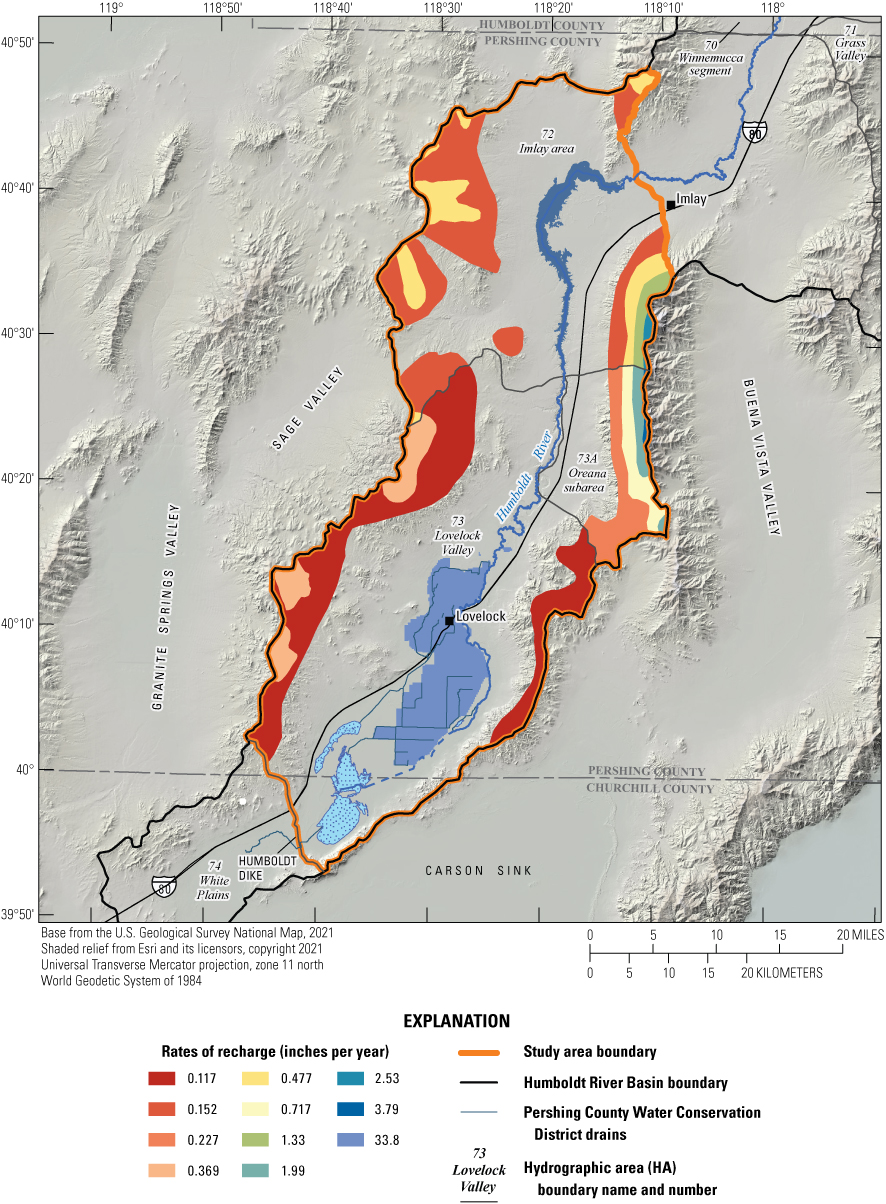
Recharge rates (from mountain block and applied irrigation) applied to layer 1.
Applied Irrigation
The annual rate of water application over the irrigated area in Lovelock Valley was simulated as an areal recharge flux into layer 1 of the model by distributing the total deliveries to the irrigation canals across the irrigation area. The simulation of crop ET was then used to partition irrigation water and shallow groundwater between crop consumptive use and groundwater recharge (as detailed in the “Groundwater Evapotranspiration” section). Minimal continuous data exist during the period of the transient simulation (1960–2016), with the exceptions of the Imlay gage, Below Rye Patch gage, and the Rye Patch Reservoir gage. It was therefore necessary to extrapolate rates of deliveries to irrigation canals from known fluxes through the Below Rye Patch gage.
A regression was developed from historical data from the years 1944 to 1961 (Everett and Rush, 1965) relating the flow released from Rye Patch Reservoir to canal deliveries for normal/dry years (defined here as Rye Patch releases less than 165,000 acre-ft/yr; fig. 5). This regression was then used to estimate annual deliveries from known fluxes through the Below Rye Patch gage for the years extending through 2016. The regression was not considered appropriate for wet years (Rye Patch releases greater than or equal to 165,000 acre-ft/yr) because an increasing proportion of flow is allowed to discharge to the Humboldt Sink once crop irrigation needs are satisfied (Everett and Rush, 1965). Additionally, very wet years can result in somewhat unpredictable changes in management of flow through the reservoir and river to prevent flooding, particularly when the capacity of the reservoir is expected to be exceeded. As such, wet year deliveries were estimated to be a constant 135,000 acre-ft/yr, assuming an application of 4.5 ft over 30,000 acres of irrigated cropland, based on historical wet-year application rates (Everett and Rush, 1965). This application rate was simulated as an areal recharge flux using the MODFLOW RCH Package (Harbaugh, 2005). Annual flow released from the Rye Patch Reservoir and the corresponding annual estimated deliveries to the irrigation canals based on the methods described above are shown on figure 6. For the steady-state calibration model, the median estimated application of surface-water irrigation from 1960 to 1990 was simulated as an areal recharge flux at a rate of 127,783 acre-ft/yr.
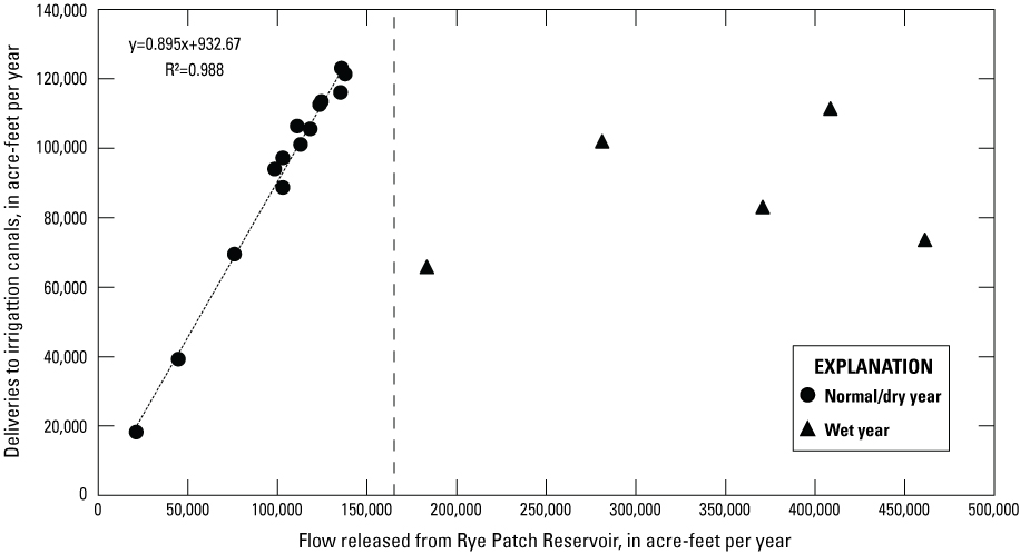
Flow released from Rye Patch Reservoir relative to deliveries to irrigation canals for normal/dry and wet years from 1944 to 1961. Dashed line indicates transition between dry/normal and wet years, defined as greater than 165,000 acre-feet per year flow released from Rye Patch Reservoir. Data are from Everett and Rush (1965). The regression equation and R2 value are listed in the upper lefthand corner.
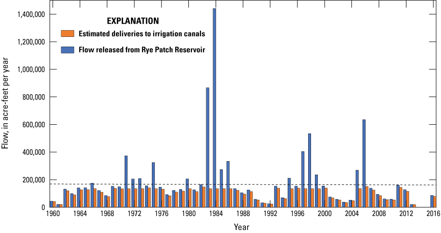
Flow released from Rye Patch Reservoir and the corresponding estimated deliveries to the irrigation canals for 1960–2016. Dashed line indicates transition between dry/normal and wet years, defined as greater than 165,000 acre-feet per year flow released from Rye Patch Reservoir.
Groundwater Evapotranspiration
For the purposes of modeling, ETg estimates were made separately for non-agricultural and agricultural ETg. Historical annual agricultural ETg was estimated based on Mapping EvapoTranspiration at high Resolution with Internalized Calibration (METRIC) net actual evapotranspiration data (total ET less precipitation over the irrigated area) from 2001 to 2011 (Huntington and others, 2018). METRIC estimates ET from the energy balance of net short and longwave radiation and heat transmitted into and out of the land surface, based on Landsat satellite data. While METRIC data represents ET, it was used for this study as a proxy for ETg. This was done because all applied irrigation was simulated as an areal recharge flux. In reality, when irrigation water is applied to agricultural fields, it first infiltrates the soil and moves through the vadose zone. Crops primarily extract infiltrating groundwater from the vadose zone to meet their water requirements before it reaches the water table. By simulating all applied irrigation water as areal recharge, the model bypasses the vadose zone processes, but by using METRIC ET as a proxy for ETg, the groundwater flow budget is maintained in terms of simulated sources and sinks. For the remainder of the report, ET simulated in the agricultural area will be referred to as ETg, because it is being simulated as such.
For the years 2001–11, METRIC net ET rates were used directly. For all other years, agricultural ETg had not been quantified, and it was necessary to develop a relationship between the volume of water applied to cropland and the rate of agricultural ETg. A comparison of estimated annual deliveries to canals and METRIC net agricultural ET rates for 2001–11 shows an apparent offset of approximately 3 years (fig. 7A). This offset may be because of the alternation between drier and wetter years observed in the 2001–11 period. When a dry year follows a wet or normal year, crops may subsist on existing soil moisture or groundwater for a limited time. Similarly, when a wet year follows a dry year or drought period, it may take time for crops to return to their former vigor. After an extended dry period, fields may need to be replanted altogether, in which case the observed lag between irrigation deliveries and agricultural ETg may represent the time required for new crops to grow to their full size. A regression was then developed relating a 3-year rolling average of irrigation deliveries to annual agricultural ETg (fig. 7B), and annual agricultural ETg rates were then estimated during the years 1960–2000 and 2012–16 based on this regression. The steady-state agricultural ETg rate was estimated using this same regression, using the steady-state applied irrigation rate of 127,783 acre-ft/yr in place of the 3-year rolling average of irrigation deliveries required by the ETg regression. Steady-state agricultural ETg was then estimated to be 105,880 acre-ft/yr, and this number was targeted during calibration of the steady-state model.
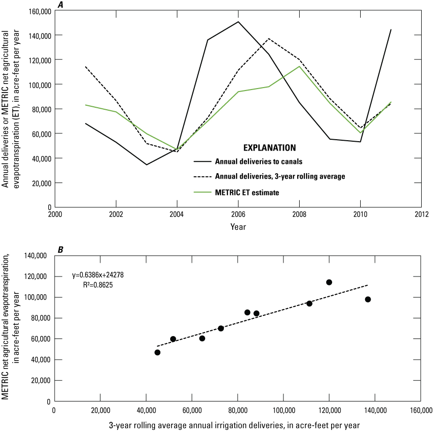
A, Relationship between estimated annual deliveries to irrigation canals, 3-year rolling average of annual deliveries to canals, and Mapping EvapoTranspiration at high Resolution with Internalized Calibration (METRIC) groundwater evapotranspiration (ETg) estimates for 2001–2011; and B, Linear regression of METRIC ET estimates and 3-year rolling average of deliveries used to estimate agricultural ETg; the regression equation and R2 value are shown.
Non-agricultural ETg includes bare soil, phreatophytes, and riparian ET; it was likewise simulated using the MODFLOW Evapotranspiration (EVT) Package (Harbaugh, 2005), assigning a calibrated maximum rate of ETg and extinction depth over polygons defined by Huntington and others (2022; fig. 8). Discussed in more detail in Huntington and others (2022), it should be noted here that adjustments were made to the initial assessment of phreatophyte ETg south of the agricultural area because the phreatophytes there are largely fed by irrigation runoff from drains and ditches (Huntington and others, 2018). This flow was removed from the model and the process was effectively short-circuited because the drains were simulated using the MODFLOW Drain (DRN) Package (Harbaugh, 2005), which simulates a groundwater outflow and does not directly simulate surface flow through the drains and ditches. Rates of phreatophyte ETg along the paths of drains and ditches were therefore reduced from the initial estimated values to avoid double counting this flow. Using this method, non-agricultural ETg within the model domain was estimated to be approximately 19,840 acre-ft/yr.
Evapotranspiration zones over the model domain as defined in Huntington and others (2022).
Humboldt River
The Humboldt River was simulated using the MODFLOW River (RIV) Package (Harbaugh, 2005) in two segments to prevent overlap with Rye Patch Reservoir. The northernmost segment extends from the Imlay gage to the eastern boundary of reservoir, and the southernmost segment extends from the Below Rye Patch gage to the Below Big Five Dam gage to the south. For the steady-state model, median water surface elevations from 1960 to 1990 were used for the Imlay and Below Rye Patch gages (U.S. Geological Survey, 2018). The median recorded water surface elevation from 1951 to 1958 was used for the Below Big Five Dam gage (U.S. Geological Survey, 2018), where data were more limited.
Flow through the Humboldt River within the Lovelock portion of the model domain can be conceptualized by a simple mass balance equation:
whereQRP
is the flow at Below Rye Patch gage;
QC
is irrigation water delivered to canals;
QR
is the net loss from the river to groundwater; and
QB5
is the flow at the Below Big Five Dam gage, discharging to the Humboldt Sink (fig. 9).
Of the four terms in equation 1, only QRP is known for the simulated period with any certainty. Irrigation water delivered to canals has been estimated as described in the “Applied Irrigation” section of this report, and the partitioning of simulated flow between QR and QB5 was derived using a similar method through analysis of historical estimates.
Conceptualized Humboldt River flow budget components for Below Rye Patch Reservoir (eq. 1), showing flow at Below Rye Patch gage (QRP), deliveries to irrigation canals (QC), loss to groundwater (QR), and flow at the Below Big Five Dam gage to the Humboldt Sink (QB5).
Historical flow estimates for 1942–61 (Everett and Rush, 1965) show a wide variability in loss from the Humboldt River (QR), ranging from –276 acre-ft/yr (a net gain) to 12,606 acre-ft/yr. As noted in Everett and Rush (1965), it seems likely that much of this variability results from dam management practices that control river water residence times within the channel. For example, the highest reported annual river loss estimate of 12,606 acre-feet (acre-ft) occurred during a typical water year with Rye Patch releasing 137,700 acre-ft. For comparison, the river actually showed a slight gain of 276 acre-ft from bank storage during a wet year when 408,600 acre-ft was released from Rye Patch. This can probably be explained by the rapid drainage of the reservoir to the Humboldt Sink to prevent flooding in the reservoir, whereas in normal/dry years, water might be held within the river channel for much of the irrigation season.
River loss estimates from 1942 to 1961 are plotted against estimated river channel flow after deliveries to irrigation canals (in other words, QRP−QC) and displayed on figure 10. A meaningful relationship could not be developed when incorporating estimates for all years, but a regression of estimates for normal and dry years only (QRP less than 165,000 acre-ft/yr) indicated a correlation between river channel flow and river loss (R2=0.7279). This regression was used to estimate annual river losses from estimated channel flow (QRP−QC) for normal and dry years for the years extending through 2016. For wet years (QRP greater than or equal to 165,000 acre-ft/yr), there was no apparent relationship between channel flow and river loss, and wet year river loss for 1960–2016 was therefore estimated based on the mean ratio (0.018) of river loss to channel flow after deliveries to canals (QRP−QC) for wet years from 1942 to 1961. Estimated river losses relative to estimated channel flow for 1960–2016 are presented on figure 11. River loss for the steady-state model was estimated at 9,900 acre-ft/yr based on the steady-state median discharge from Rye Patch Dam and corresponding estimated deliveries to irrigation canals. Because of the difference in the relationship of flows through Rye Patch Dam, deliveries to canals, and river loss between normal/dry and wet years, median flows through Rye Patch Dam are not correlated with median deliveries to canals or with median river loss rates. The targeted value of 9,900 acre-ft/yr for steady-state river loss is therefore higher than the mean and median estimated river loss for 1960–90 (7,300 and 8,400 acre-ft/yr, respectively). The river was calibrated by varying the conductance term, which is a lumped parameter defined as the product of the streambed hydraulic conductivity and the length and width of the stream reach, divided by the thickness of the riverbed material.
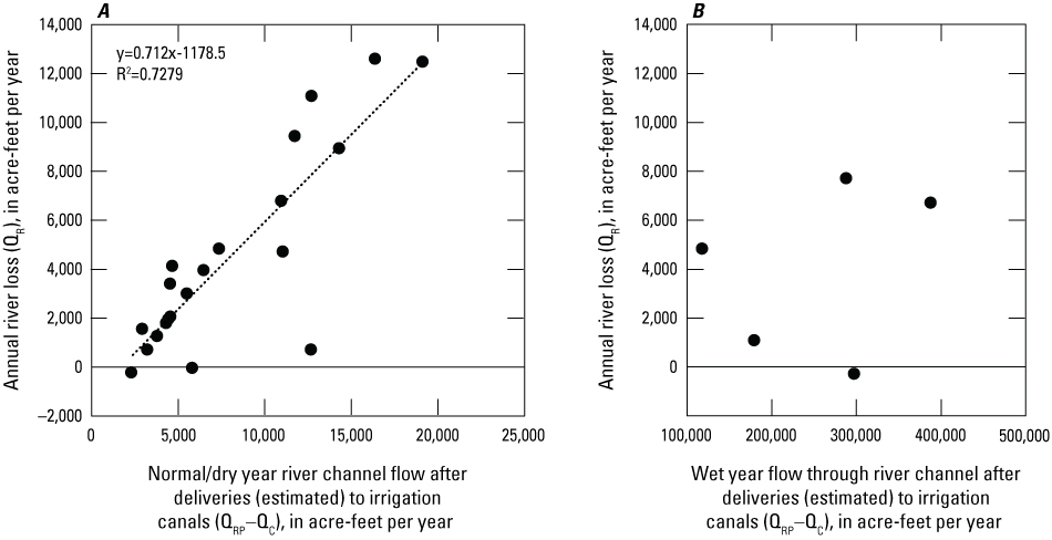
River channel flow after estimated deliveries to irrigation canals (QRP−QC) relative to annual river losses in the Humboldt River (QR) for A, normal/dry years and B, wet years from 1944 to 1961. Data are from Everett and Rush (1965). Note difference in scale on horizontal axis. The regression equation and R2 value are listed in the upper lefthand corner of figure A.
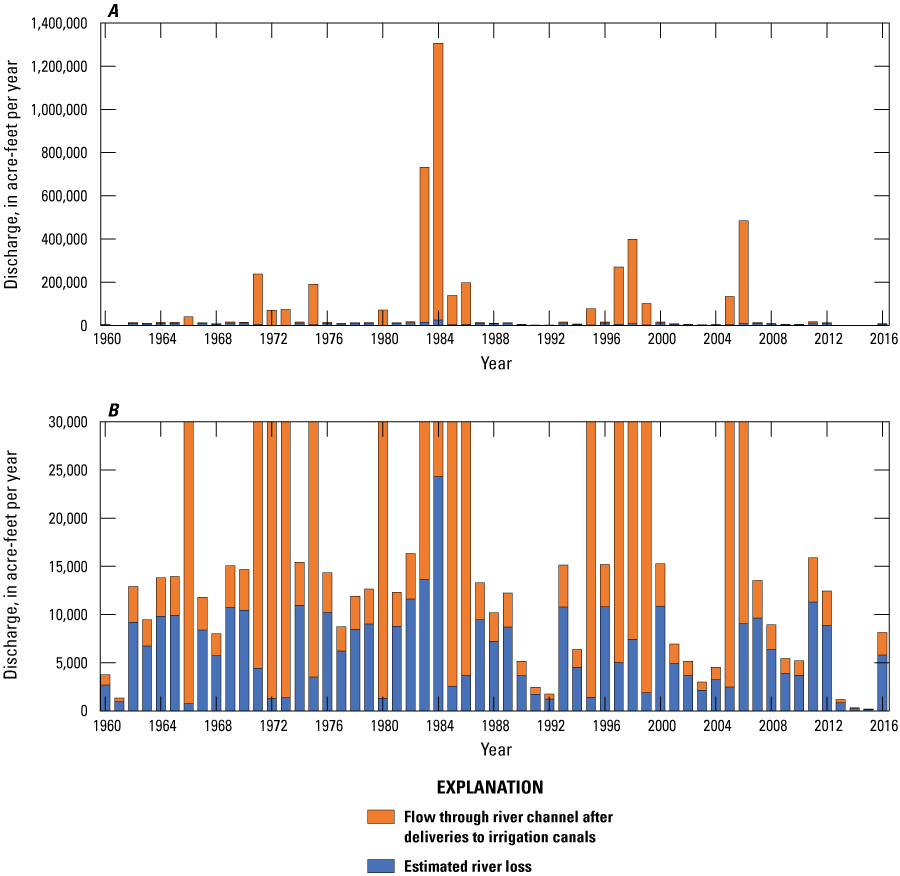
Estimated river loss to groundwater from the Humboldt River relative to the total remaining flow through the river channel after deliveries to irrigation canals. Figures A and B show the same data at different y-axis scales for context.
For the historical transient simulation, the recorded median annual stage was assigned to the Imlay and Below Rye Patch gages for each stress period. Intermittent stage data at the Big Five Dam gage were limited to the years 1998–2000. To estimate median annual river stage at this point, a rating curve was developed from the available data (fig. 12; U.S. Geological Survey, 2018). Estimated annual flows through the Big Five Dam gage (QRP–QC–QR) were then used to calculate a median stage for each year in the transient simulation.
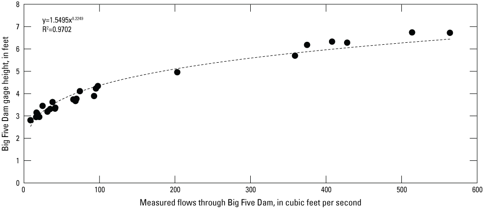
Rating curve relating measured flows to gage height at Big Five Dam between 1998 and 2000. The regression equation and R2 value are listed in the upper lefthand corner.
Rye Patch Reservoir
Lakes within the model domain include Rye Patch Reservoir, the Upper and Lower Pitt-Taylor Reservoirs, Toulon Lake, and Humboldt Lake (also referred to as the Humboldt Sink; fig. 1). Of these, only Rye Patch Reservoir is explicitly simulated, because the others are frequently dry and underlying groundwater levels have not been measured or are downgradient of the developed portions of the study area. Rye Patch Reservoir is simulated as a constant head boundary using the MODFLOW Time-Varying Constant Head (CHD) Package (Harbaugh, 2005) for the steady-state and transient models, using the median stage from 1960 to 1990 for the steady-state model and the median annual stages for the transient simulation. Previous studies have estimated that bank storage associated with Rye Patch Reservoir changes between 6,000 and 14,000 acre-ft/yr on average (Eakin, 1962; Fereday and Nash, 2017), where bank storage is defined as water temporarily held within the banks or bed of the reservoir to be later released back to the reservoir during periods of lower water levels. As Rye Patch Reservoir water levels decline during irrigation season, water is gained from bank storage. When it fills during off-irrigation season, water is lost from the reservoir to bank storage. These fluctuations are seasonally cyclical and can be skewed by very wet or dry years (Fereday and Nash, 2017). However, no estimates have been made on permanent Rye Patch Reservoir loss to groundwater, where seepage through the banks or bed of the reservoir reaches the water table to recharge the aquifer and flow downgradient, rather than returning to the reservoir. Rye Patch Reservoir loss to groundwater was assumed to be some fraction of average change in bank storage, and 14,000 acre-ft/yr was therefore used as the upper bound on simulated reservoir loss to groundwater during model calibration.
Interbasin Flow
Interbasin flow from the portion of the Imlay area east of the Imlay gage was simulated as a specified flux boundary using the MODFLOW Well (WEL) Package (Harbaugh, 2005) in layers 1 and 2 along the eastern edge of the model domain in the Imlay Basin (fig. 13) and is limited to the area of basin-fill deposits. The model boundary in the Imlay Basin is simulated to receive 760 acre-ft/yr groundwater flow into the model. All other model boundaries were simulated as no-flow.
Locations of irrigated cropland, specified flux boundary, and drains in Lovelock Valley.
Canals and Drains
In practice, a network of canals is used to divert water from the Humboldt River and deliver it to irrigated cropland in Lovelock Valley. Although it is likely that some amount of flow through the canals is lost to groundwater before reaching irrigated cropland, the rate of loss is unknown and likely highly variable. Because the canals mainly run between and adjacent to the irrigated area, all delivered water was assumed to have been applied to the fields as part of the term for applied irrigation; thus, canals were not explicitly simulated.
Similarly, a series of drains extends across the irrigated area (fig. 13). Fields in this area are routinely irrigated above crop water requirements with the intention of flushing precipitating salts from the root zone. Drains, dug to a depth of 8–10 ft, prevent the fields from becoming water-logged and deliver this excess water to Toulon Lake and the Humboldt Sink (Everett and Rush, 1965). Few measurements of drain flow have been made, and none have encompassed all drain flow for a single year. Everett and Rush (1965) estimated groundwater outflow to drains to be 21,000 acre-ft/yr, based on the difference between estimated water applied to crops and estimated use by irrigated crops. Drains were simulated using the MODFLOW DRN Package (Harbaugh, 2005) with a depth of 9 ft and an estimated steady-state drain discharge of 18,360 acre-ft/yr, which was determined as the sum of all inflows less ET. Drains were calibrated by varying the conductance, which is a lumped parameter that describes the head losses between the drain and the surrounding aquifer and dictates the rate of groundwater flow to the drain from the groundwater system. All simulated drains were assumed to have the same unit length conductance.
Faults
In order to improve simulation of spatial variability in measured groundwater levels, one fault was represented in the model using MODFLOW’s Horizontal Flow Barrier (HFB6) Package (Harbaugh, 2005), coinciding with the range front fault bounding the Humboldt Range in the Imlay area (HA 72; fig. 14). Faults within the model domain were identified from a geologic map (Johnson, 1977), but no other mapped fault in the area had sufficient groundwater-level data to determine whether it might be affecting groundwater flow.
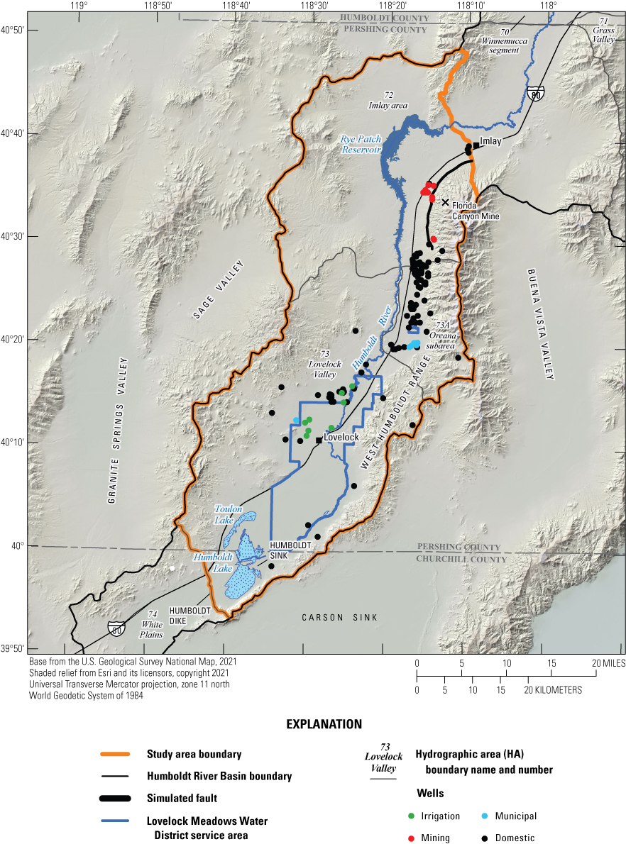
Locations of a simulated fault, the Lovelock Meadows Water District service area, and wells pumped in the transient simulation.
Well Withdrawals
Very little pumping occurs within the simulated area, largely because of poor water quality in Lovelock Valley (Everett and Rush, 1965). Municipal wells providing drinking water to the Lovelock area are in the Oreana subarea (HA 73A) and typically pump less than 1,500 acre-ft/yr (Jon Benedict, State of Nevada Division of Water Resources, retired Hydrogeologist, written commun., 2017). A few irrigation wells are in central/northern Lovelock Valley where the water quality is adequate for irrigation; these wells are permitted as supplemental to river water. In the simulated portion of the Imlay area, most pumping supports operations in the Florida Canyon Mine, which is along the base of the Humboldt Range east of the river. This pumpage is less than 1,500 acre-ft/yr during the simulated period (figs. 14, 15).
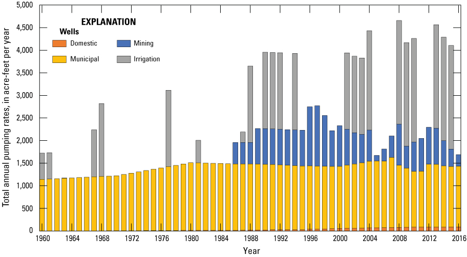
Total annual pumping rates for domestic, municipal, mining, and irrigation wells for 1960–2016 in the transient simulation.
Municipal and mining wells were pumped at reported rates for all years between 1994 and 2016 (fig. 15; Jon Benedict, State of Nevada Division of Water Resources, retired Hydrogeologist, written commun., 2017). Before 1994, total municipal pumping was extrapolated backwards to 1960 according to population records and was distributed amongst whichever wells were in operation for each year, with guidance from permitting records. The earliest known pumping rates for mining wells at Florida Canyon also were extrapolated backwards to when the mine first became operational in 1986, with attention to the completion dates of pumped wells. Domestic wells throughout the model domain were assumed to pump at 0.7 acre-ft/yr, beginning in the year they were completed and continuing through the end of the simulated period. The rate of 0.7 acre-ft/yr was selected based on domestic pumping rates for nearby hydrographic areas from pumpage inventories (State of Nevada Division of Water Resources, 2018). Most domestic wells within Lovelock Valley are no longer in use due to poor water quality and were therefore excluded from the simulation within the Lovelock Meadows Water District (LMWD) service area (Everett and Rush, 1965; fig. 14). Domestic wells within the LMWD service area that were drilled after 1995 were assumed to be active, and pumping was simulated from these wells.
No official records of pumping rates for irrigation wells in Lovelock Valley exist for the simulated period. Because all irrigation water rights in this area are supplementary to surface water, irrigation pumping was assumed to be inversely proportional to applied irrigation. For years in which estimated applied irrigation met or exceeded the median for 1960–90, irrigation wells were not pumped. For years in which estimated applied irrigation was less than the 1960–90 median, irrigation wells were pumped at the fraction of missing recharge multiplied by the water right at that well. For example, if the applied irrigation rate was 90 percent of the median, irrigation wells would be simulated as pumping at 10 percent of their water right. This method resulted in substantially more pumping from irrigation wells from 1990 to 2016 than in previous years; however, because these rates were already small, the maximum estimated total pumping in the model domain did not exceed 4,700 acre-ft for any year (fig. 15).
Calibration
Model calibration is an important step in the development of many groundwater models that simulate a real-world groundwater system. For a model to be used to answer questions about a given system or to be used in a predictive role, it must first be shown to adequately simulate observed behavior in that system within a reasonable margin of error. Calibration is the iterative process of adjusting simulated input parameter properties, which are not known with certainty (such as hydraulic conductivity or storage parameters) until the computed solution matches observed values to a reasonable level of accuracy. For this study, the model was calibrated to observed groundwater levels and estimated fluxes, including loss to groundwater from the Rye Patch Reservoir and the Humboldt River, agricultural and non-agricultural ET, and groundwater outflow to drains. Observed groundwater levels were used to inform simulated heads. The terms heads and groundwater levels are used interchangeably in the following model calibration sections.
Steady-State Calibration
Model parameters calibrated in the steady-state model include hydraulic conductivities, river and drain conductances, maximum ET rates, and extinction depths. The steady-state model was calibrated using a combination of automated Parameter ESTimation software (Doherty and Hunt, 2010) and manual calibration, targeting the estimated flow rates for each flow budget component described in this report and groundwater levels obtained from well logs. For the purposes of the model described in this report, the steady-state period was defined as any time before 1960—however, the number and spatial distribution of logs from wells drilled before 1960 were extremely limited. Because pumping rates within the model domain were relatively low for the duration of the simulated period (fig. 15), it was assumed that the water table had not changed significantly over time and thus additional groundwater-level data from well logs collected after 1960 were used. For these wells, data were limited to wells drilled during non-wet years to more closely approximate average conditions.
Hydraulic conductivities for the majority of the model domain were parameterized based on the surface geology described by Maurer and others (2004) and displayed on figure 2. To reduce model complexity in areas and form a basis for calibration where little data existed, the surface geologic units were grouped into hydrogeologic zones based on rock type and location. In layers 1 (Lahontan clays and silts) and 2 (underlying coarser younger and older alluvium combined), the hydraulic conductivity for a portion of unconsolidated material in Lovelock Valley HA was parameterized through interpolation of pilot point values using the aquifer test results presented in Nadler (2020) for the region affected by the extent of drawdown of those tests (fig. 3). For unconsolidated materials in this area but outside of the aquifer test drawdown region, hydraulic conductivity was initially defined at pilot points based on specific capacity results from well logs. For these points, hydraulic conductivities were allowed to vary within the range of hydraulic conductivities defined by the aquifer test results. Hydraulic conductivity was allowed to vary separately for layers 1 and 2. Final values for hydraulic conductivities throughout the model domain were estimated from iterative calibration between the steady-state and transient models, to minimize the difference between observed and simulated heads and flows and to optimize replication of observed trends in heads in the transient model. Simulated hydraulic conductivities ranged from 0.0001 feet per day (ft/d) in the basement bedrock in layer 3 to 100 ft/d in layer 2 in the Lovelock Valley agricultural area and are presented for each layer on figures 16–18. In both layers 1 and 2, calibrated hydraulic conductivities are generally lower for unconsolidated materials in the northern portion of the study area compared to the southern portion of the study area where values were controlled by interpolated pilot points. Hydraulic conductivity values in the northern portion of the study area were determined solely by model calibration and not by data from aquifer tests and specific capacity values from well logs. The hydraulic characteristic (defined as the hydraulic conductivity of a barrier divided by its width) of the Imlay area fault delineated on figure 14 was calibrated alongside aquifer hydraulic conductivities to a value of 1.62x10⁻⁶ days–1 to match observed groundwater-level elevations more closely in that area.
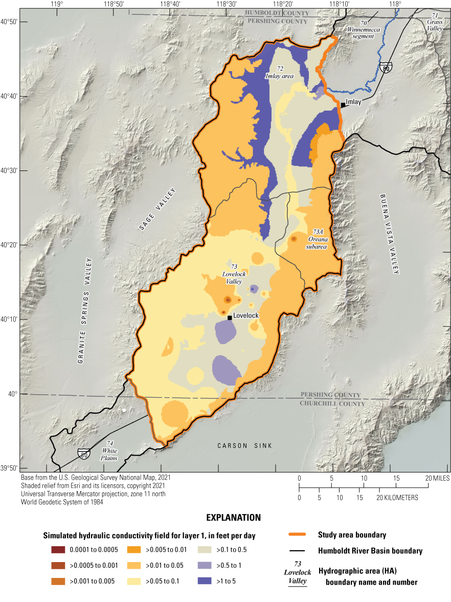
Simulated hydraulic conductivity field for layer 1.
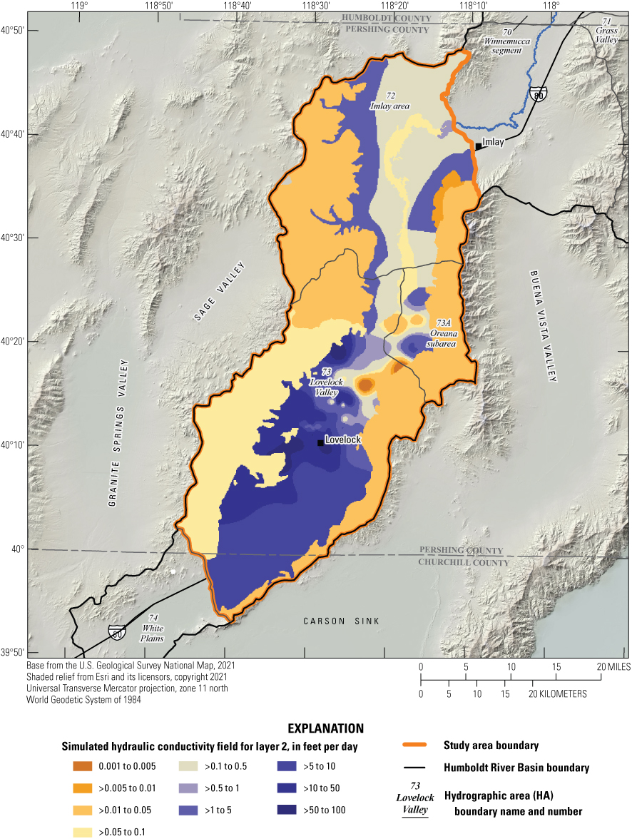
Simulated hydraulic conductivity field for layer 2.
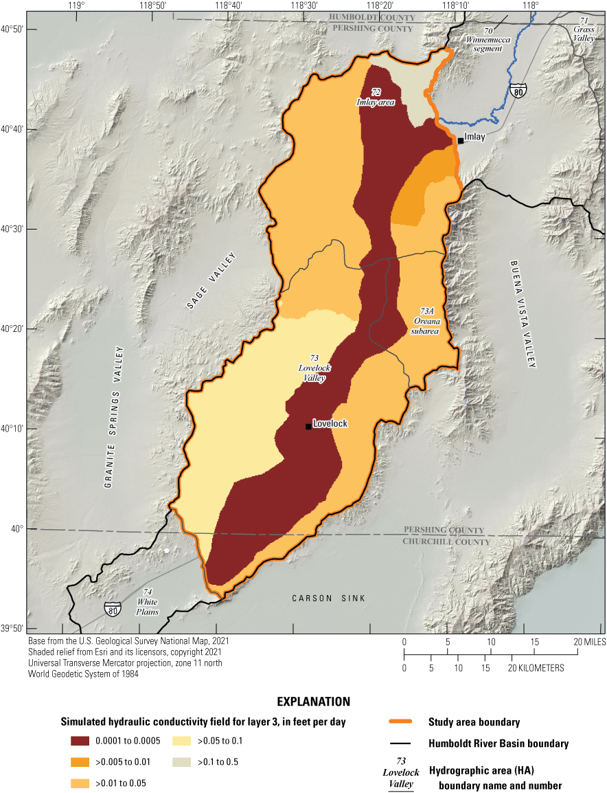
Simulated hydraulic conductivity field for layer 3.
River conductance was calibrated targeting the estimated steady-state net flow into the model (river loss) of 9,900 acre-ft/yr. The final unit length conductance value for the river was set to 30 (ft2/d)/ft, with a total inflow from the river of 10,930 acre-ft/yr and total outflow to the river of 998 acre-ft/yr—for a net estimated recharge from the river into the model of 9,932 acre-ft/yr.
Maximum ETg rates and extinction depths were calibrated individually by ETg type (bare soil, phreatophytes, riparian, and irrigated cropland) and by HA. Targeting the estimated steady state rate of 105,800 acre-ft/yr for the irrigated cropland region, the final simulated agricultural ETg rate was 106,693 acre-ft/yr, with a maximum potential ETg rate of 4.4 feet per year (ft/yr). The extinction depth for the agricultural ETg type was set to 9 ft, based on the depth of the drains, assuming the high total dissolved solids in groundwater in Lovelock Valley (HA 073; Everett and Rush, 1965) would inhibit root growth beyond the depth routinely flushed by the drains. Targeting the estimated steady-state rate of 19,840 acre-ft/yr, the final simulated bare soil, phreatophytes, and riparian ETg rate was 18,810 acre-ft/yr, with maximum potential ETg rates ranging from 1.5 to 4.4 ft/yr, and extinction depths ranging from 5 to 45 ft. Simulated maximum potential ETg rates and extinction depths are itemized by hydrographic basin and ETg type in table 3, and a comparison of targeted and final simulated rates by HA and ETg type is presented on figure 19.
Table 3.
Estimated maximum evapotranspiration rates and extinction depths for all simulated sources of evapotranspiration in the model domain, by hydrographic area and evapotranspiration type determined through calibration.[ETg, groundwater evapotranspiration; ft/yr, foot per year; ft, foot]
Shown in figure 1.
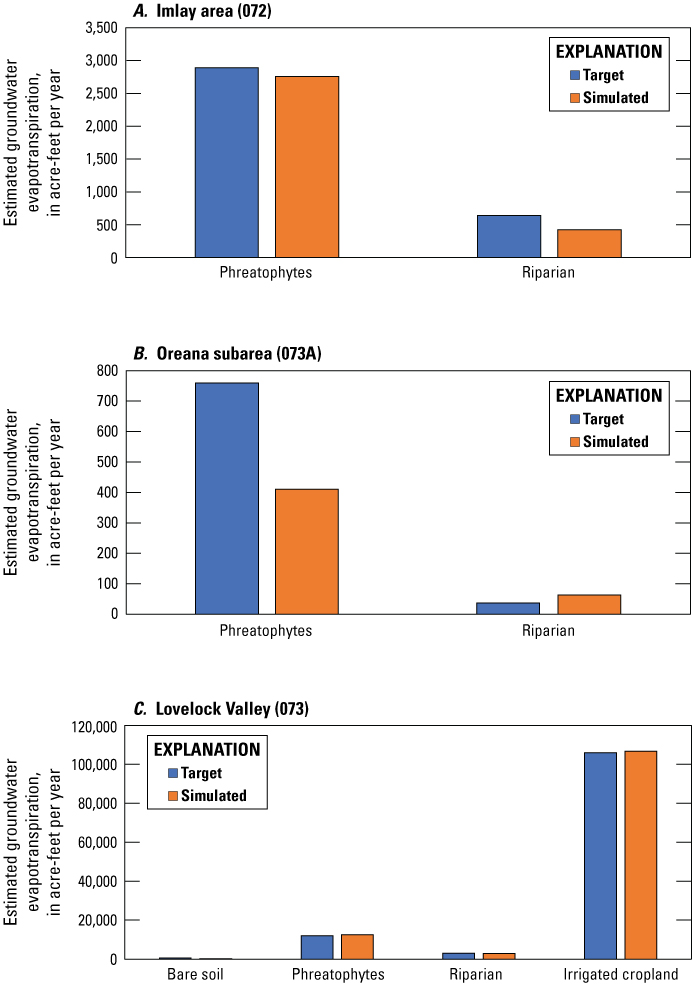
Targeted estimated groundwater evapotranspiration (ETg) rates compared to simulated ETg for A, the Imlay area, B, the Oreana subarea, and C, Lovelock Valley hydrographic areas, by evapotranspiration type within the lower Humboldt River Basin study area.
The Rye Patch Reservoir was simulated as a constant head boundary, which does not include a conductance term to be calibrated explicitly. Instead, flow into and out of a constant head boundary is determined by the difference between the assigned head and the heads in the surrounding grid cells and the hydraulic conductivities of those grid cells. Steady-state model calibration to local heads and ETg rates resulted in a net loss to groundwater from the reservoir of 63 acre-ft/yr, well within the upper limit of 14,000 acre-ft/yr defined in the “Rye Patch Reservoir” section of this report.
Drain conductance was calibrated targeting a steady-state flow rate equal to total model inflows (recharge, interbasin flow, river loss, and reservoir loss) less ETg. The final unit length conductance value was set to 40 (ft2/d)/ft, with a total outflow of 18,360 acre-ft/yr. Although measured outflows to all drains are not available, this outflow is comparable to the estimate of 21,000 acre-ft/yr provided by Everett and Rush (1965).
Final calibration of the steady-state model resulted in a mean head residual of –2.51 ft, a mean absolute head residual of 17.84 ft, and a root mean square head residual of 27.24 ft, equating to a relative error of 1.5 percent over an observed range of heads of 1,214 ft. The spatial distribution and magnitude of head residuals are shown on figure 20, and a comparison of simulated and observed heads is shown on figure 21.
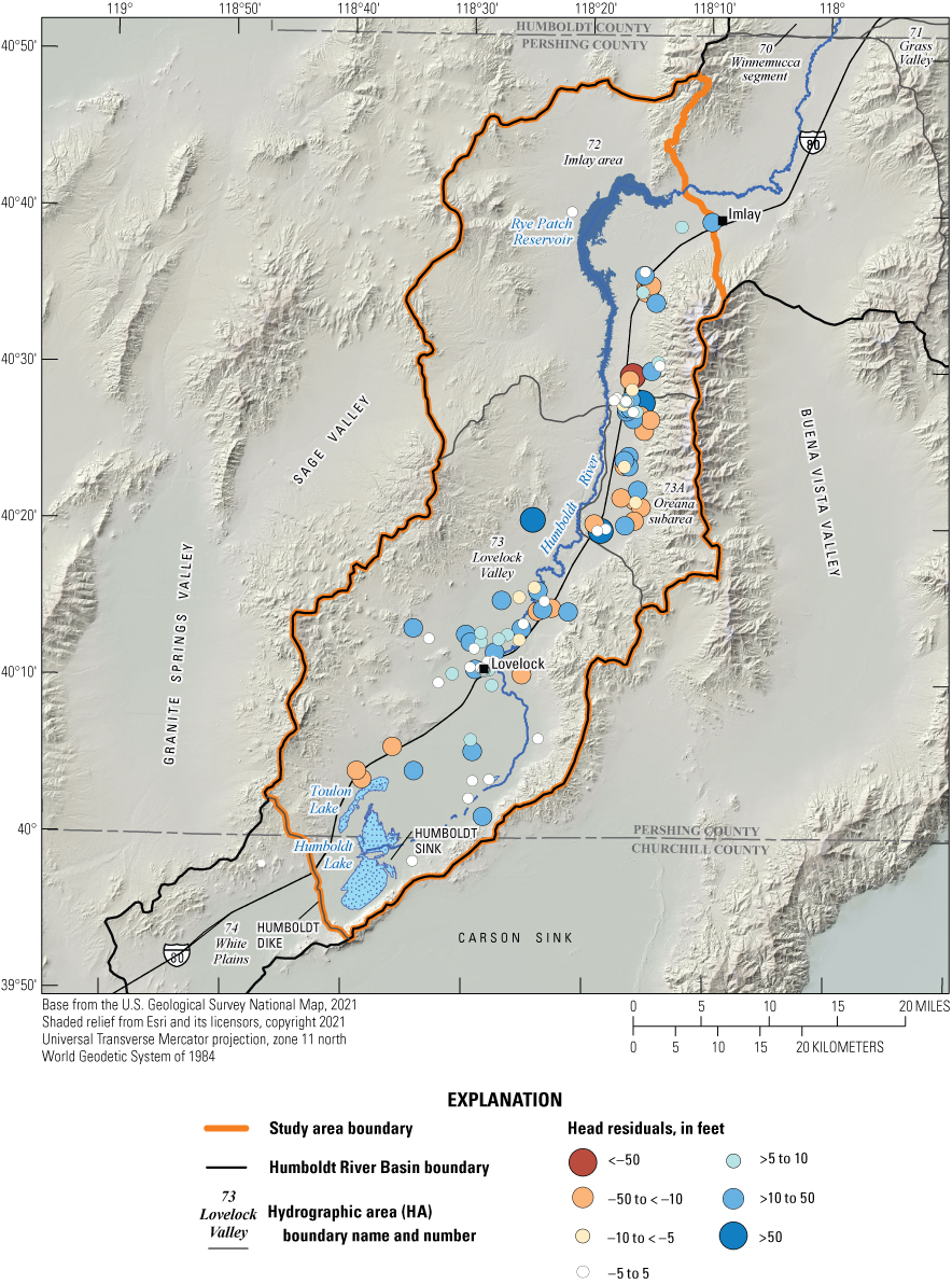
Head residuals for the calibrated steady-state model within the lower Humboldt River Basin study area. Red/orange circles indicate areas where simulated heads are less than measured heads, and blue circles indicate areas where simulated heads exceed measurements.
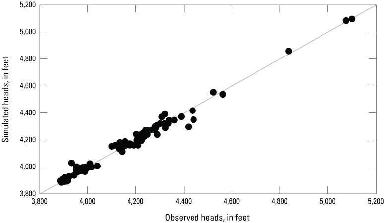
Comparison of simulated and observed heads from the calibrated steady-state model within the lower Humboldt River Basin study area, plotted along a one-to-one line.
Transient Calibration
The transient model was developed to calibrate storage parameters for use in the capture analysis. In the Lower Humboldt Basin, very little transient groundwater-level data exist. Groundwater-level data were collected for 100 wells from the Nevada Division of Water Resources (Nevada Division of Water Resources, 2018), with most records beginning in the mid-to-late 2000s, though records extend back to the early-to-mid 1990s for 3 wells owned by the Lovelock Meadows Water District. Storage parameters were manually calibrated to trends in observed heads and were assigned to the same zones used for hydraulic conductivities. Final values for specific storage for layers 1 and 2 were 0.00002 per foot (ft–1) for the regions of consolidated rock and 0.0003 ft–1 in the basin fill, and they are presented on figure 22. Specific storage for layer 3 was set to 4.0x10⁻⁶ ft–1. Plots of simulated and observed heads at selected locations throughout the basin (near Rye Patch Reservoir, the Florida Canyon Mine, Lovelock Meadows municipal wells in the Oreana subarea, and near the irrigated cropland in Lovelock Valley; fig. 23) are shown on figures 24–26.
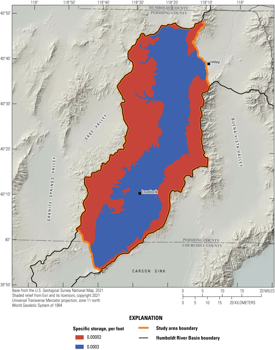
Specific storage values applied to the Lahontan clays and silts (layer 1) and the combined underlying coarser younger and older alluvium (layer 2) within the lower Humboldt River Basin study area.
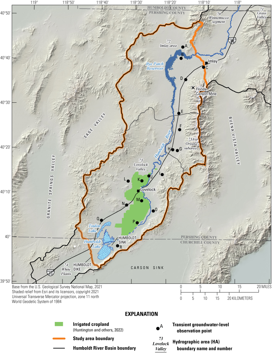
Locations of transient groundwater-level observations throughout the lower Humboldt River Basin study area. Plots of the simulated and observed groundwater levels for these locations are shown on figures 24–26.
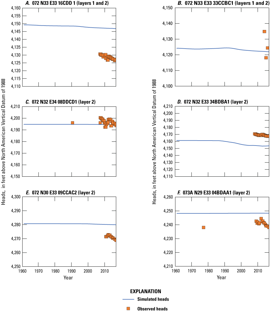
Simulated and observed heads for the transient historical model at points A, 072 N33 E33 16CDD1 (layers 1 and 2); B, 072 N33 E33 33CCBC1 (layers 1 and 2); C, 072 N32 E34 08DDCD1 (layer 2); D, 072 N32 E33 34BDBA1 (layer 2); E, 072 N30 E33 09CCAC2 (layer 2); and F, 073A N29 E33 04BDAA1 (layer 2; fig. 23) in the Imlay area and northern Oreana subarea. Plots are annotated with the layers intersected by the observation well screened interval.
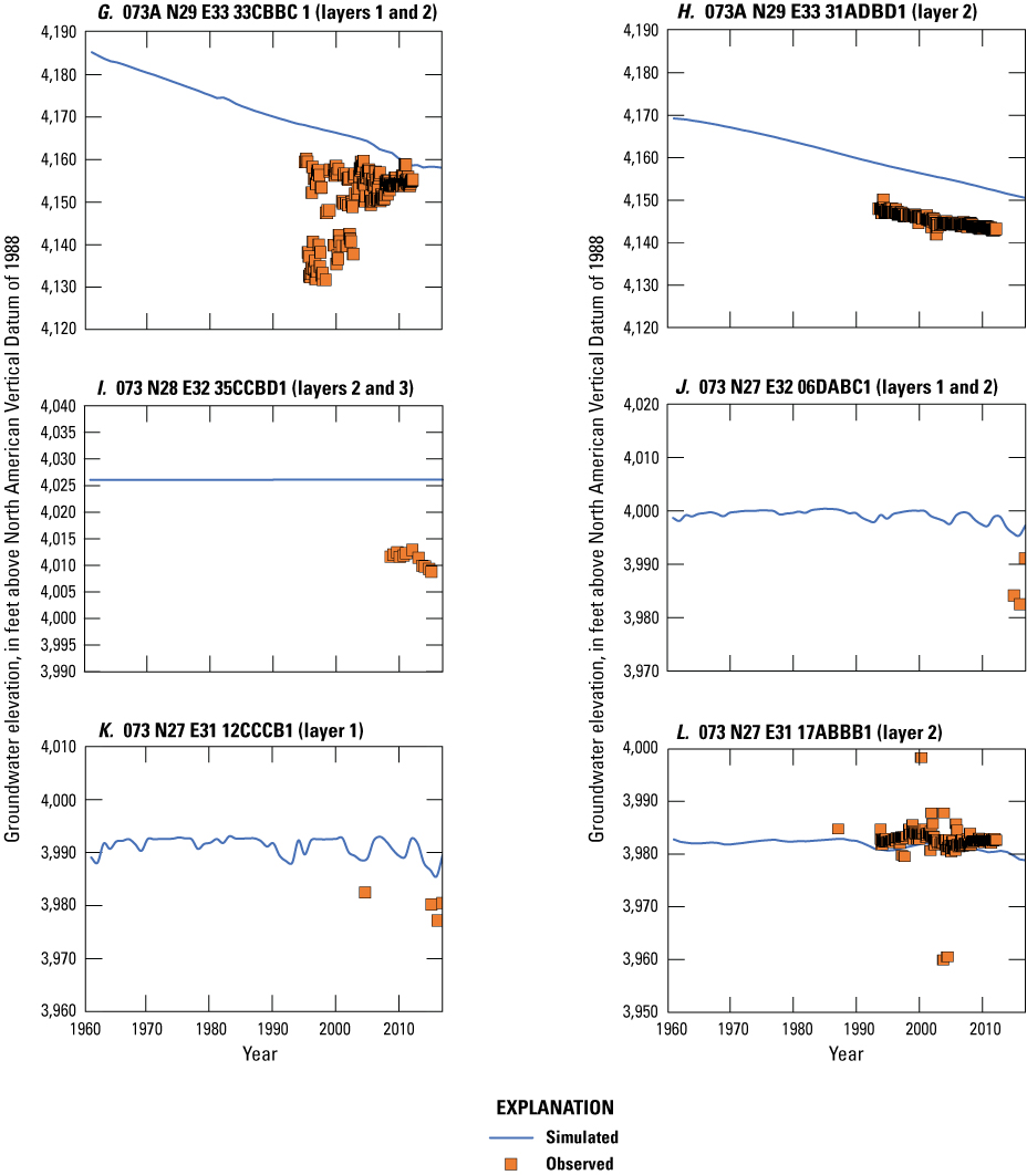
Simulated and observed heads for the transient historical model at points G, 073A N29 E33 33CBBC1 (layers 1 and 2); H, 073A N29 E33 31ADBD1 (layer 2); I, 073 N28 E32 35CCBD1 (layers 2 and 3); J, 073 N27 E32 06DABC1 (layers 1 and 2); K, 073 N27 E31 12CCCB1 (layer 1); and L, 073 N27 E31 17ABBB1 (layer 2; fig. 23) in the southern Oreana subarea and central Lovelock Valley. Plots are annotated with the layers intersected by the observation well screened interval.
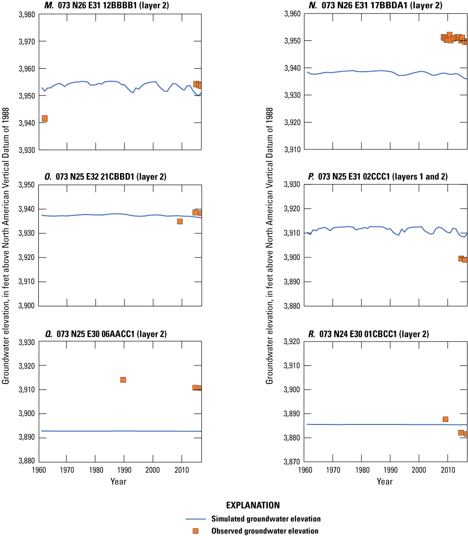
Simulated and observed heads for the transient historical model at points M, 073 N26 E31 12BBBB1 (layer 2); N, 073 N26 E31 17BBDA1 (layer 2); O, 073 N25 E32 21CBBD1 (layer 2); P, 073 N25 E31 02CCC1 (layers 1 and 2); Q, 073 N25 E30 06AACC1 (layer 2); and R, 073 N24 E30 01CBCC1 (layer 2; fig. 23) in central and southern Lovelock Valley. Plots are annotated with the layers intersected by the observation well screened interval.
Within the Imlay area (locations A–E on fig. 23), observed heads indicate little to no change for the 2007–16 period, and this condition is well represented by simulated heads (figs. 24A–E). In the Oreana subarea (locations F–H on fig. 23), a decline in heads of about 0.26 ft/yr has been observed in the area of the Lovelock municipal wells during the 1992–2013 period (figs. 24F, 25G–H). This trend is well simulated; however, simulated heads are approximately 5–10 ft higher than observed. Note that the observed heads plotted on figure 25G include some measurements taken when the well was pumping. These short-term fluctuations could not be simulated given the annual stress periods used in the model. Instead, simulated trends should be compared to measurements taken after the well had recovered. Near the agricultural area in Lovelock Valley (locations I–R on fig. 23), observed heads fluctuated approximately 5 ft from 1994 to 2013, and simulated heads match these trends well (fig. 25L). Simulation results show little variability in head at this location until the beginning of the observed head oscillation in 1994, with a slight decline in more recent years (2013–16) during a drought, coinciding with a period of reduced application of surface water for irrigation. The remaining transient observation points near the agricultural area in Lovelock Valley have only a few observed heads, and a comparison of trends cannot be made. These points are included to show the simulated variability in heads at these points and the difference in observed and simulated heads where available (figs. 25J–K, 26M, and 26O–R). Final calibration of the transient historical model resulted in a mean head residual of 11.86 ft, a mean absolute head residual of 32.95 ft, and a root mean square head residual of 72.5 ft, equating to a relative error of 2.2 percent over an observed range in heads of 1,507 ft.
A comparison of transient simulated ETg to ETg estimated using the 3-year rolling average of deliveries to irrigation canals described in the “Groundwater Evapotranspiration” section of this report is shown on figure 27. Agricultural ETg is a major component of the flow budget in the study area (Everett and Rush, 1965) and is very well represented by the model.
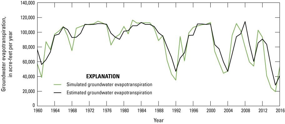
Simulated groundwater evapotranspiration from irrigated cropland from the transient model compared to estimated evapotranspiration from the Mapping EvapoTranspiration at high Resolution with Internalized Calibration (METRIC) evapotranspiration regression within the lower Humboldt River Basin study area.
A similar comparison of transient simulated river loss from the Humboldt River to estimated river loss over time, as described in the “Humboldt River” section of this report, is shown on figure 28. Although agricultural ETg is well simulated, the model is much less able to simulate the estimated river loss rates. This limitation of the model is likely a function of the package used to simulate the river (MODFLOW RIV Package; Harbaugh, 2005) and limitations in the method used to estimate river loss. River stage was varied with each stress period in the transient model to best represent the river’s effect on local heads; however, the RIV Package does not directly simulate streamflow and instead effectively acts as a perpetual source or sink of water—meaning that the simulated river can never go dry and can always accept more groundwater inflow. The conductance term was calibrated in the steady-state model based on median flow through Rye Patch Dam, and as a result, simulated transient river loss rates tend to remain steady and close to the median value. Additionally, the regression used to estimate river loss was a function of just the flow out of Rye Patch Dam less deliveries to irrigation canals, and therefore the regression could not account for important but unknown factors such as the timing of deliveries, the wetting state of the riverbed and its effect on conductance over time, and rates and volumes of exchange of river water into and out of bank storage. As a result, estimated rates of river loss are much more loosely correlated to flows out of Rye Patch Dam and deliveries to irrigation canals than are agricultural ET rates.
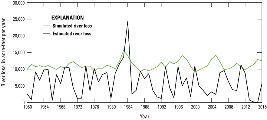
Simulated river loss from the Humboldt River to groundwater from the transient model compared to estimated river loss from the Humboldt River.
Model Limitations
The primary limitation of this model is its less precise simulation of transient river gains and losses, particularly during dry years or during years in which the basin is recovering from a dry period. Because the river is simulated using the MODFLOW RIV Package, the simulated river effectively acts as a perpetual source or sink of water to the model; this means that the simulated river can never go dry and is always available as a source of water to the aquifer. Likewise, the simulated river can always accept more water from the surrounding aquifer without causing a change in stage. Gains and losses to and from the simulated river are dependent on the stage assigned to the river and the simulated groundwater elevation in the basin. The model is further limited by the lack of streamflow data along the river flow path within the model domain, meaning there was no information available for calibration purposes regarding where along the streamflow path the river might be gaining or losing. The model therefore has limitations in its use in making future predictions in fluxes to and from the river under varying flow conditions. However, because the model is calibrated to estimated river loss during a year of median flow through the Rye Patch Dam, it is suitable for use in predictions of groundwater levels or capture under typical flow conditions.
The model is similarly limited in the area of the Rye Patch Reservoir, which is simulated using the MODFLOW CHD Package (Harbaugh, 2005). Like the simulated river, the simulated reservoir can always lose or gain water to or from the aquifer without causing a change in the reservoir stage. For this reason, the model would not be appropriate for evaluating predictive drawdown at a well near the reservoir. This boundary condition is suitable for the purposes of this study because simulated wells used to generate capture percentages are pumped at low rates that would not be expected to affect the stage of the reservoir enough to impact the capture percentage.
Another limitation is in the methodology used to define the surface-water elevation of the Humboldt River. Surface-water elevations were defined at point locations. These points were placed at locations where surface-water measurements were available, including the Below Rye Patch gage, the Below Big Five Dam gage, and dams in the Lovelock agricultural area for which construction information was available. Surface-water elevations were interpolated between these points. For each of these points, only one surface-water elevation was simulated, causing any drop in stage occurring at a dam location to not be represented in the model, except at the Below Rye Patch gage where both the stage of Rye Patch Reservoir and the stage downstream at the Below Rye Patch gage are captured. River water levels were averaged over ‘steps’ in the surface-water elevations, which could mean that the stage of the river is underestimated or overestimated in the model in some locations. Simulated gains and losses from the Humboldt River are a function of the prescribed surface-water elevation relative to the simulated groundwater levels in adjacent model cells, meaning that an overestimation of the Humboldt River stage could result in an overestimation of river losses to groundwater.
The model also is limited by the lack of information regarding the timing and location of mountain block recharge. Mountain block recharge is applied simply according to the precipitation zones delineated in Hardman and Mason (1949). However, this method is most appropriate for estimating total mountain block recharge for a hydrologic area, and the spatial zones more accurately represent the area upon which precipitation initially falls. This assignment of mountain block recharge does not account for the fraction of recharge that first becomes runoff, entering a hydrologic area as recharge along an alluvial fan or even further downgradient within a basin. Aquifer parameters therefore have greater uncertainty in and adjacent to the mountain block.
The model is similarly limited by sparse information on the timing and location of irrigation pumping. Irrigation pumping was assumed to be inversely proportional to the applied irrigation rate, which may be an overestimation because poor groundwater quality in the irrigated area of Lovelock Valley may prohibit irrigation during years where the ratio of mixed river water to pumped groundwater is too low to reduce dissolved solids to a level that can be tolerated by crops. With no additional information, a conservative pumping rate was assigned to these wells.
The model also is limited by the lack of hydraulic conductivity and storage property data for much of the model domain, outside of the area of Lovelock Valley where aquifer tests were conducted in support of this model. Model results are therefore most reliable in and near the irrigated area of Lovelock Valley and other locations with more substantial groundwater withdrawals.
All layers in the model domain were simulated as confined based on the conceptual model of a clay confining layer (layer 1) overlaying a more transmissive layer of sands and gravels (layer 2). With this conceptualization, model calibration resulted in a specific storage value for layer 2 (0.0003 per ft) that was greater than what would be expected for a confined aquifer, which was required to match fluctuations in observed groundwater levels. This indicates the system may actually be unconfined, or leaky confined, which over a long enough period may be represented as an unconfined system. While the model calibration reasonably matches observed groundwater levels, the high storage parameter assigned to layer 2 may result in an underestimation of stream capture. Possible future work could revisit the conceptualization of the aquifer.
Capture Analysis
Capture, as first described by Theis (1940), is the change of inflow to or outflow from a groundwater system caused by groundwater pumping. Numerous studies have revisited and expanded upon the concept of capture (Bredehoeft and others, 1982; Leake and others, 2008; Leake and others, 2010; Barlow and Leake, 2012; Davids and Mehl, 2014; Konikow and Leake, 2014; Nadler, 2016; Nadler and others, 2017). At the onset of pumping, water is removed from aquifer storage as drawdown surrounding the well (the cone of depression) extends outward. This drawdown and depletion of stored groundwater continues until the hydraulic gradient between the well and a source of recharge, discharge, or both, changes. This change allows the pumping to intercept or “capture” a flow of water eventually equal to the pumping rate (Theis, 1940; Barlow and Leake, 20122). In time, the groundwater levels at and surrounding the well will continue to decline with pumping until the rate of capture is equal to the pumping rate of the well. When this occurs, groundwater levels stabilize, and the aquifer has reached a new state of equilibrium. Groundwater captured by a pumping well may come from multiple sources (capture sources), such as stream capture and ETg capture. Stream capture is the combination of induced seepage from streams into the groundwater system and decreased discharge from the groundwater system into streams. In this study, the term stream capture describes capture from the Humboldt River and Rye Patch Reservoir. Salvaged ETg as a source of capture is the diversion of water to a pumping well that would otherwise have naturally discharged via ETg. Capture can be described in volumetric terms (volumetric capture rate) or it can be expressed as a percentage of groundwater pumping rate causing the change (capture percentage). The source and rate of capture is often determined through use of groundwater flow models (Leake and others, 2010).
A capture analysis can be used to calculate capture that has historically taken place (historical capture) and to predict capture that could potentially take place in the future (predictive capture). Historical stream capture can be estimated with a numerical groundwater flow model by comparing changes in river flux between a calibrated transient model representing actual historical pumping (the historical model) and the same model with historical pumping removed. Any change in river flux between the two model runs can be attributed to actual groundwater pumping that has taken place and has resulted in stream capture. This kind of analysis can be done for any source of water to wells. Predictive capture can be estimated with the same methods as historical capture but applied to the predictive model. That is, a predictive model can be based on a calibrated historical model that is extended into the future to examine a future stream capture scenario. The predictive model is then run for a specified period with future predicted pumping and with no pumping. The difference in river flux between the two model runs is the predictive stream capture that can be attributed to the predicted pumping simulated to take place.
Historical and predictive capture can be estimated for existing well locations, but the potential or hypothetical capture at any given location requires a different type of analysis. Potential capture can be estimated with a capture model— having a base case model run and numerous hypothetical pumping well model runs. The base case model run represents predicted hydrologic conditions with a fixed amount of background pumping. The hypothetical pumping model runs are identical to the base case run, except for the addition of one well that pumps at a specified rate per model run in locations of interest. In this study, the comparison is done for every model cell. The difference in river flux between the base case model run and each individual hypothetical well model run is the potential capture that can be attributed to each hypothetical well location. Potential capture percentages, once calculated at given locations in a system at given points in time, can be contoured to produce a capture map as a visual aid to describe spatial variations in the relative amount of potential stream capture over time (Cosgrove and Johnson, 2005; Leake and others, 2008; Peterson and others, 2008; Leake and others, 2010). Capture maps provide spatiotemporal information on how a new or existing well would potentially source its capture in an easily interpreted visual format. Capture maps are typically developed using automated methods. The methods used in this study to create capture maps for the lower HRB are described by Leake and others (2010).
Historical, predictive, and potential capture were all calculated for the lower HRB with the three distinct models described above. Historical capture was estimated with the historical model, predictive capture was estimated with the predictive model, and potential capture was calculated with numerous capture models. The lower HRB capture analyses evaluate stream capture, drain capture, ETg capture, and changes in groundwater storage. Changes in leakage terms in the MODFLOW RIV Package from the Humboldt River and in the MODFLOW CHD Package from Rye Patch Reservoir together comprise stream capture for the study area. Stream leakage, ETg, drains, and storage terms are calculated for each annual timestep of the transient model.
Historical and Predictive Capture
Historical stream capture from existing pumping was estimated for the period 1960–2016 using the historical model (a modified version of the calibrated transient historical model). The historical model was used to simulate the system with and without the existing pumping well distribution. Predictive stream capture from 2017 through 2116 for the pumping wells that existed in 2016 was estimated using the predictive model (a modified version of the calibrated transient model). The predictive model starting heads are the ending heads from the transient historical model. The boundary conditions in the predictive model are represented with median historical values defined in the historical model, except for mountain block recharge and background pumping. Mountain block recharge is represented using rates from the steady-state calibration model. Predicted pumping was represented by mean historical pumping rates as defined in the 1960–2016 transient pumping record. Mean pumping values were considered a more reasonable estimate of future pumping than pumping during any single recent year or set of years because historical pumping varied widely year to year. For example, as illustrated in figure 15, irrigation wells in the valley that pump with supplemental water rights are principally pumped during dry years when there is an insufficient amount of water from the Humboldt River available for irrigation use. Additionally, mining wells were only pumped for some of the years in the historical period. For the predictive period, all non-mining existing (background) wells were pumped at their mean rates. Total mean annual pumping during the predictive period was 2,900 acre-ft/yr.
Results of the historical and predicted stream capture analyses are presented in terms of total acre-ft/yr (fig. 29) and as a percentage of the pumping rate (fig. 30). During the historical and predicted periods, stream capture comprised a very small amount of the total pumping (fig. 29), remaining at 10 percent or less of annual pumping for the entire 156 years simulated (fig. 30). Stream capture generally increased during the historical period (1960–2016) from 6 acre-ft/yr in 1960 to 252 acre-ft/year in 2016 (fig. 29). This general increase was characterized by steeper increases in dry years and intermittent declines during the wet years. Years with increased pumping had increases in stream capture rates because the higher pumping rates increased hydraulic gradients and intercepted or induced more flux to or from the Humboldt River and Rye Patch Reservoir. Groundwater levels typically recovered quickly in subsequent wet years and restored much of the groundwater storage lost during dry years to become available again as the main source of water to wells. The aquifer did not fully recover between dry years in the 2000s though, and thus historical stream capture exhibited an overall slight increasing trend. The final year simulated with historical data (water year 2016) was relatively wetter than the previous 3 years, resulting in a decrease in pumping rates but a rise in historical stream and drain capture (figs. 29, 30).
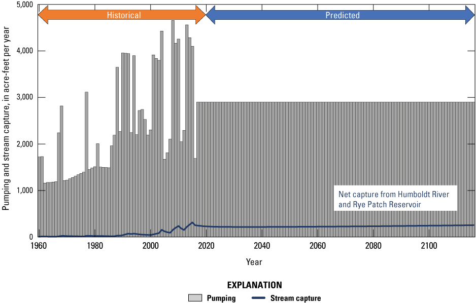
Pumping and stream capture rates for the transient historical period (1960–2016, below the orange arrow) and a 100-year predicted period (2017–2116, below the blue arrow). The blue line represents net capture from the Humboldt River and Rye Patch reservoir.
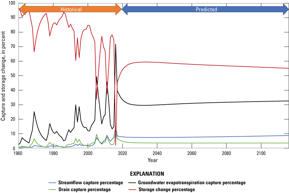
Capture and storage change percent for the transient historical period (1960–2016, below the orange arrow) and a 100-year predictive period (2017–2116, below the blue arrow).
The first year of the predictive period simulates an increase in pumping from the final historical year, thus causing a steep increase in predictive storage change percentage that is compensated by moderate decreases in predictive capture fractions from streamflow, drains, and ETg (fig. 30). After this initial change, pumping is held constant during the predictive period (2017–2116), causing trends in predictive capture and storage change fractions to generally stabilize. By the end of the predictive period, predictive stream capture accounts for only about 9 percent of water (253 acre-ft/yr) sourced to the simulated well distribution, and predictive drain capture accounts for only about 4 percent (fig. 30). During this same period, predictive ETg capture accounts for about 32 percent and predictive storage change accounts for about 55 percent of water sourced to the existing well distribution (fig. 30). The predictive model demonstrates that wells pumping in the lower HRB do not source very much water from stream or drain capture; rather, the source of water to wells is mainly storage change and ETg capture. The predictive model also demonstrates that the system is very slow to reach equilibrium (when the storage change fraction would reach 0 percent).
Potential Capture and Capture Maps
The lower HRB transient calibration model was modified to produce a hypothetical capture model used to calculate predictions of potential capture from hypothetical pumping for any given location throughout the lower Humboldt domain. A base-case model run, or reference run, was developed from the lower HRB transient calibration model where river and reservoir stages, recharge, and the maximum rate of ETg and the ETg extinction depth were held constant. The use of uniform boundary conditions helps reduce model computation time and resources. The hypothetical capture model used median rates for all boundary conditions except for mountain block recharge and background pumping. Mountain block recharge was held constant at the steady-state rate. In this modified model, all non-mining existing (background) wells were pumped at their mean rates. For municipal wells, the mean pumping rate was taken from the time they began pumping to 2016. For irrigation wells, the mean pumping rate was calculated from the year they were permitted until 2016, which includes years that supplemental wells did not pump because sufficient surface water from Rye Patch Reservoir was available. Domestic well pumping rates were set at 0.7 acre-ft/yr, which is the assumed value used in the Lower HRB transient calibration model. Only wells that were still permitted in 2016 were included in the base case model run. Background pumping was included in the analysis to ensure that the available ETg capture would diminish as it has through time, because groundwater levels have lowered from existing pumping over time.
Each flux component from the base capture model was subtracted from the same flux component from each hypothetical well model run, which simulates added groundwater pumping in an individual model cell. The difference in each flux component for each time step is the potential volumetric capture and storage change. Each capture model run included one new hypothetical capture well pumping at 476 acre-ft/yr (56,842 cubic feet per day, ft3/day), which is the median of the mean municipal pumping rate. This pumping rate was chosen to be large enough to numerically resolve changes in boundary fluxes for evaluation of capture. The potential capture analysis was performed by making 388,362 forward runs of the hypothetical capture model, each simulating the potential capture and potential storage change from a single well in one of each of the active model cells. The potential capture and storage change rates were then divided by the pumping rate of 476 acre-ft/yr to calculate time-varying potential capture and storage change percentages across the model domain. Potential capture and storage change percentages were then mapped and contoured to produce capture maps that visually characterize potential capture and potential storage change during 100 years. Potential capture and potential storage change at 1 (figs. 31–34), 10 (figs. 35–38), 50 (figs. 39–42), 75 (figs. 43–46), and 100 (figs. 47–50) years are shown and discussed below.
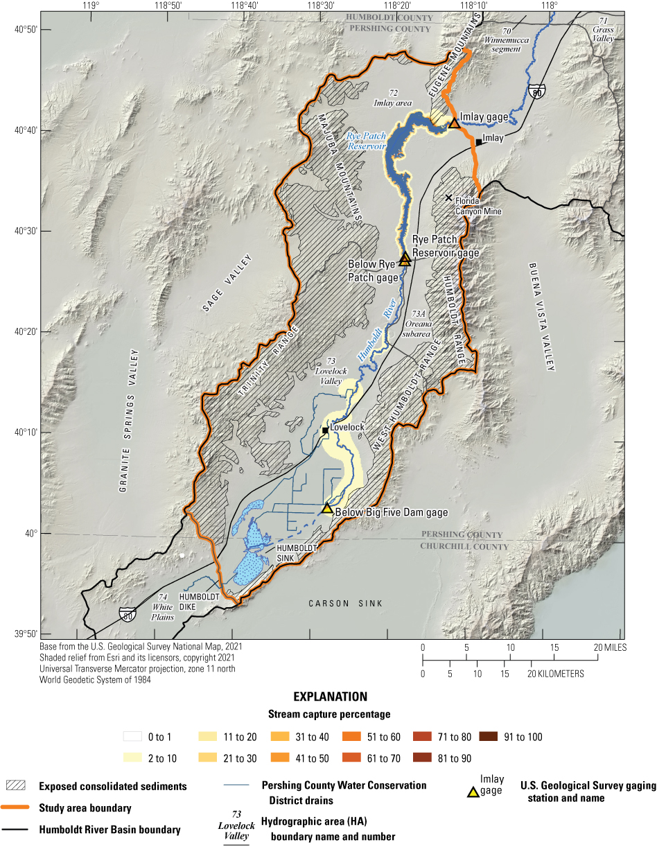
Stream capture map of layer 2 from a pumping rate of 476 acre-feet per year after 1 year of pumping.
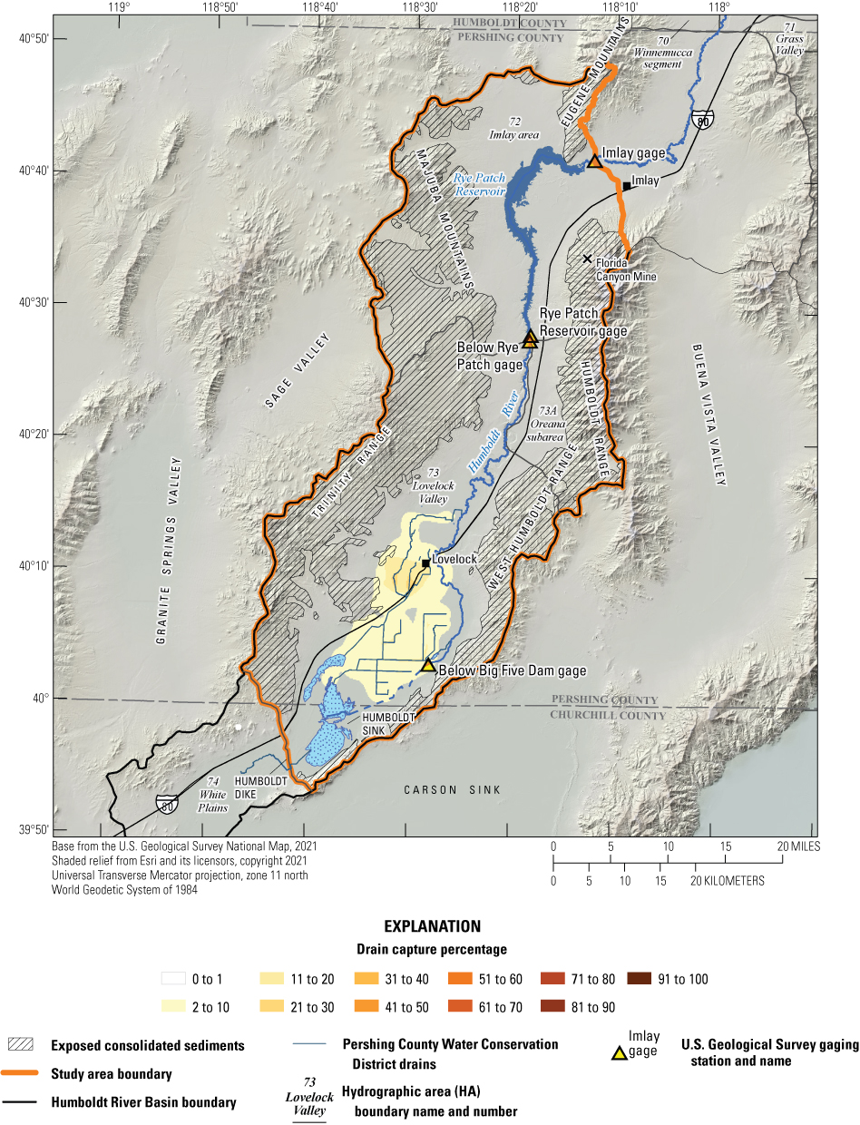
Drain capture map of layer 2 from a pumping rate of 476 acre-feet per year after 1 year of pumping.
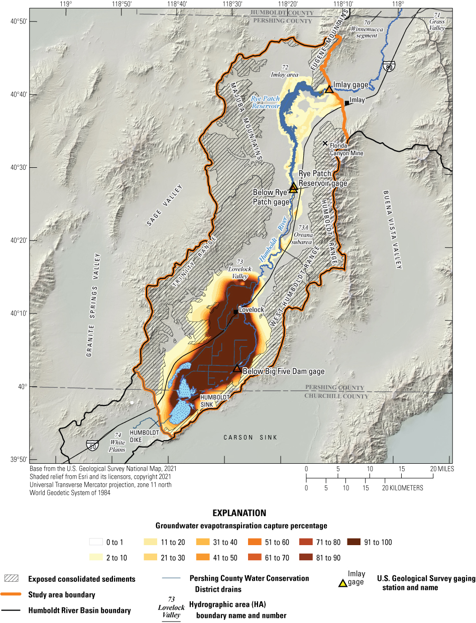
Groundwater evapotranspiration capture map of layer 2 from a pumping rate of 476 acre-feet per year after 1 year of pumping.
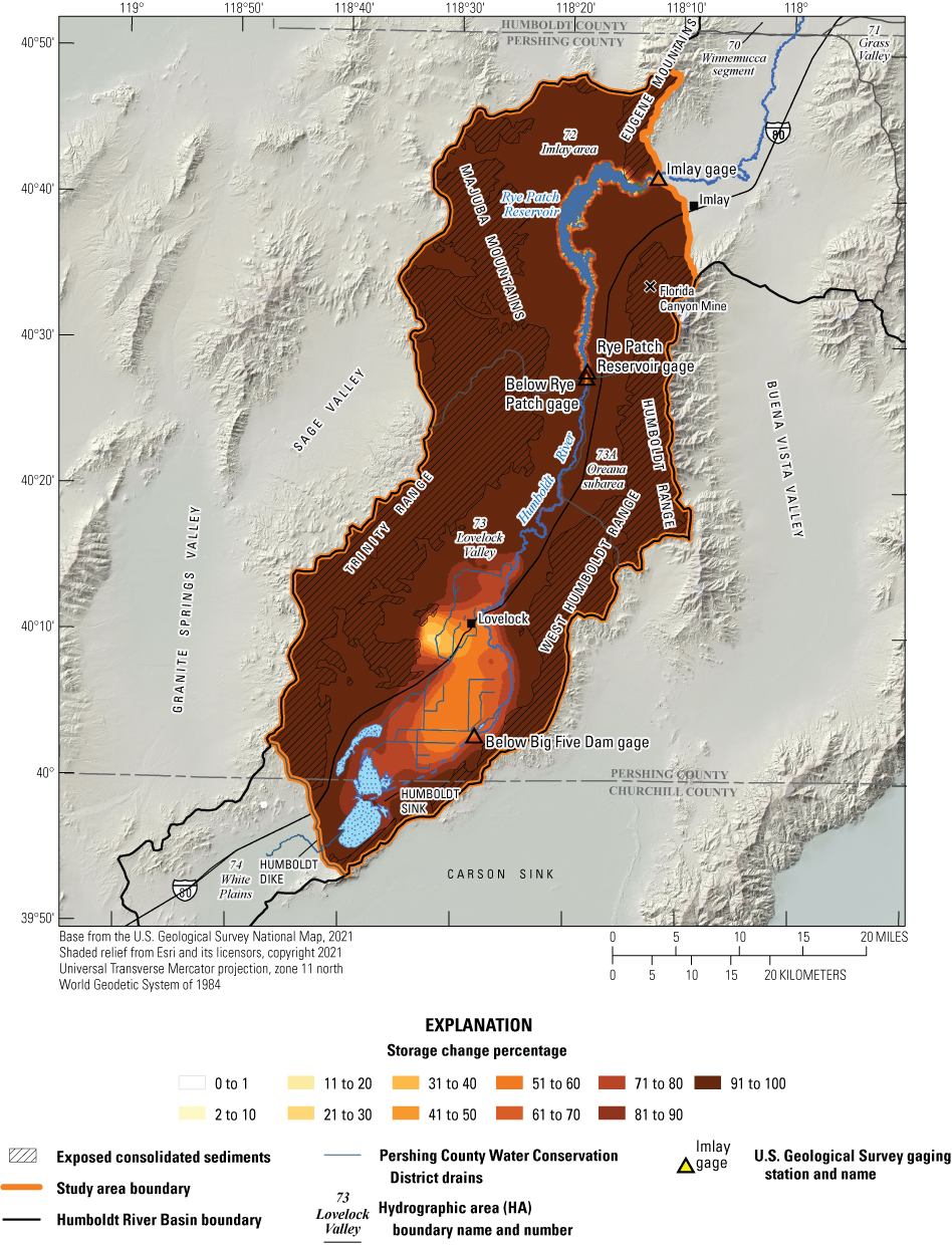
Storage change map of layer 2 from a pumping rate of 476 acre-feet per year after 1 year of pumping.
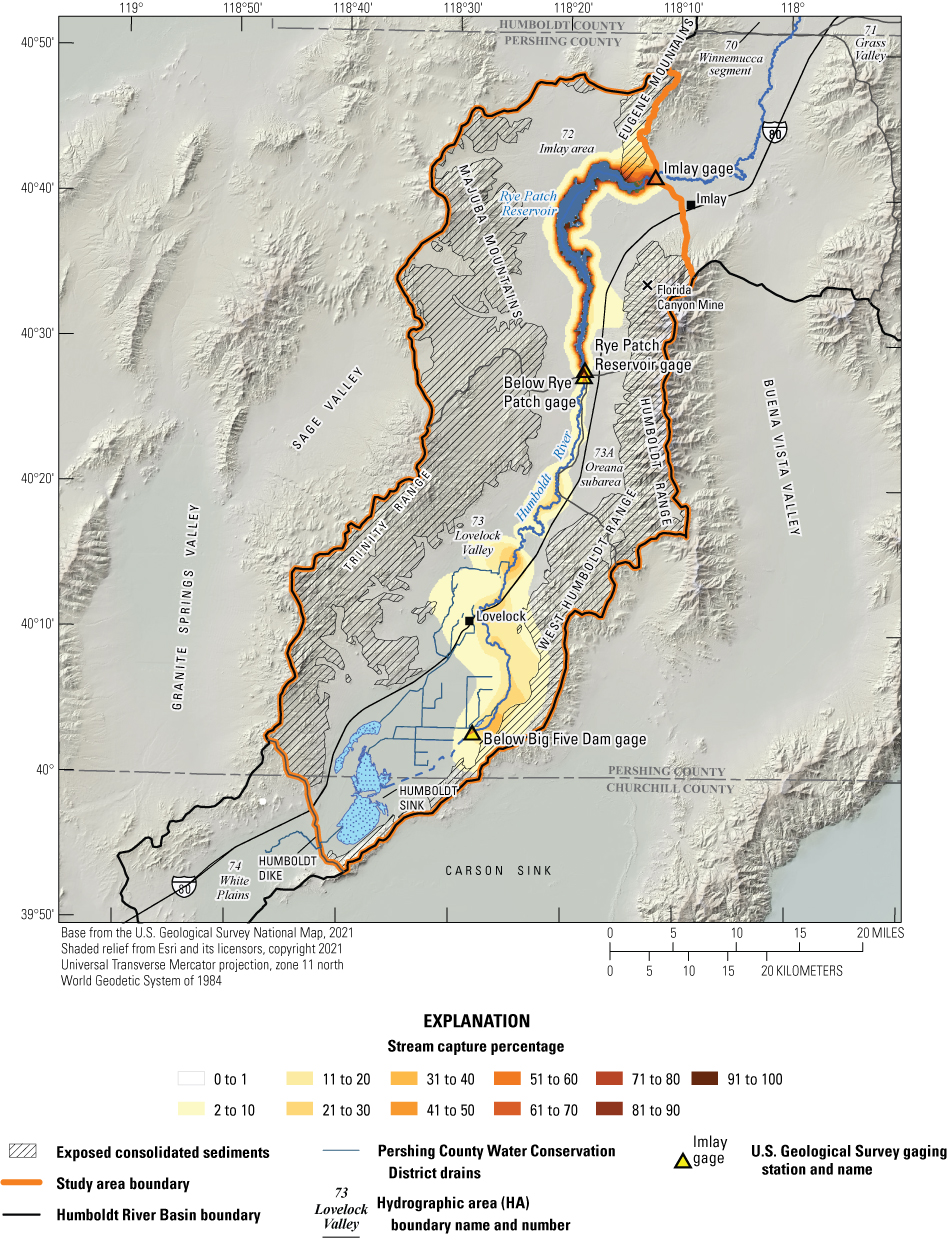
Stream capture map of layer 2 from a pumping rate of 476 acre-feet per year after 10 years of pumping.
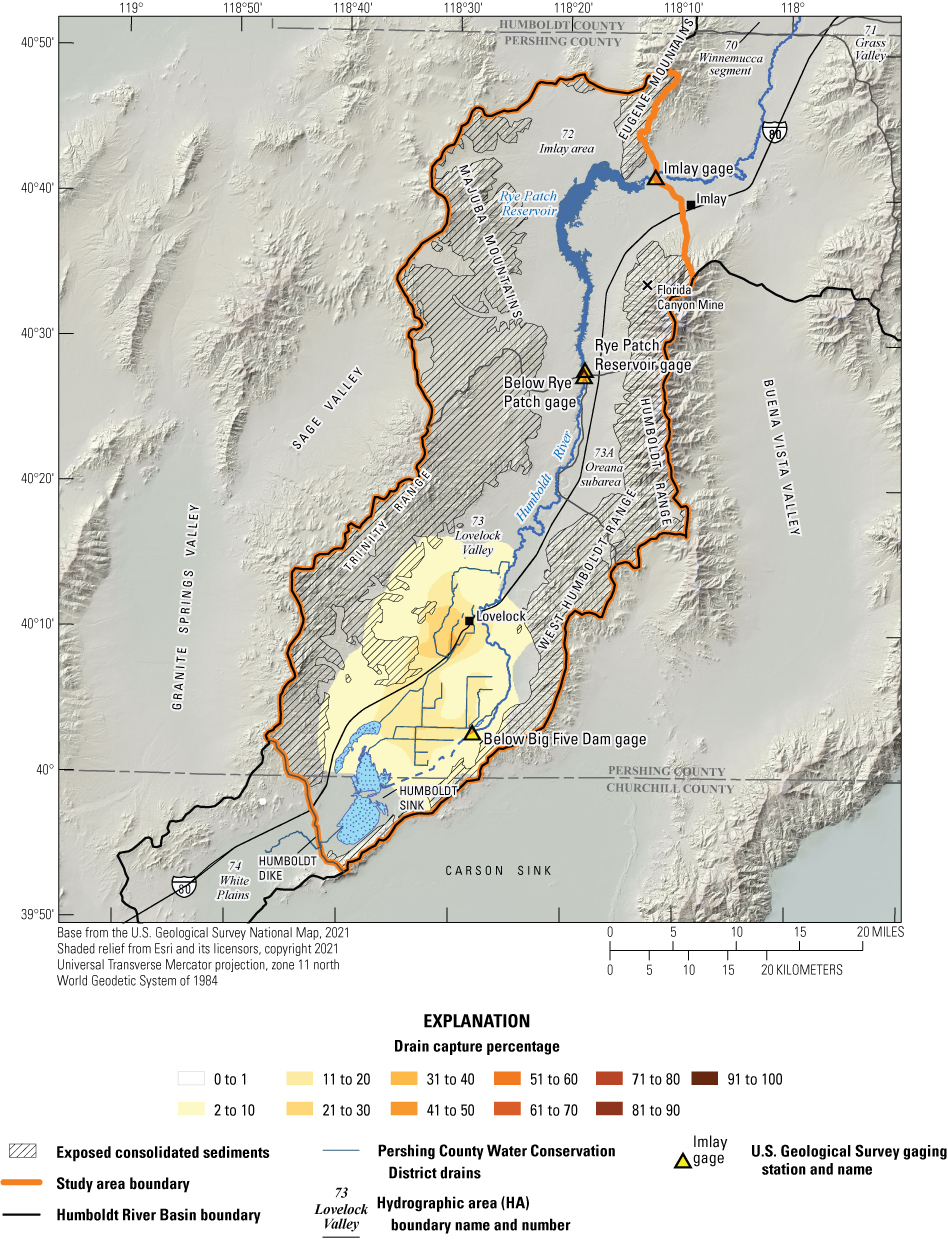
Drain capture map of layer 2 from a pumping rate of 476 acre-feet per year after 10 years of pumping.
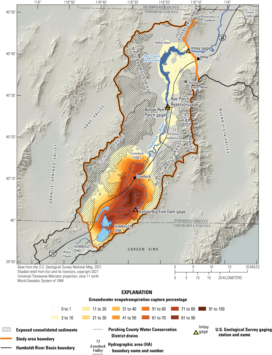
Groundwater evapotranspiration capture map of layer 2 from a pumping rate of 476 acre-feet per year after 10 years of pumping.
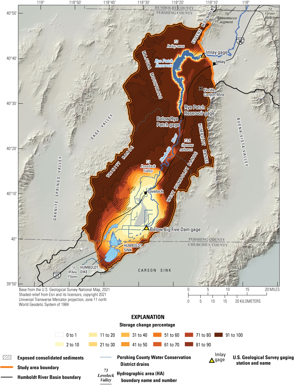
Storage change map of layer 2 from a pumping rate of 476 acre-feet per year after 10 years of pumping.
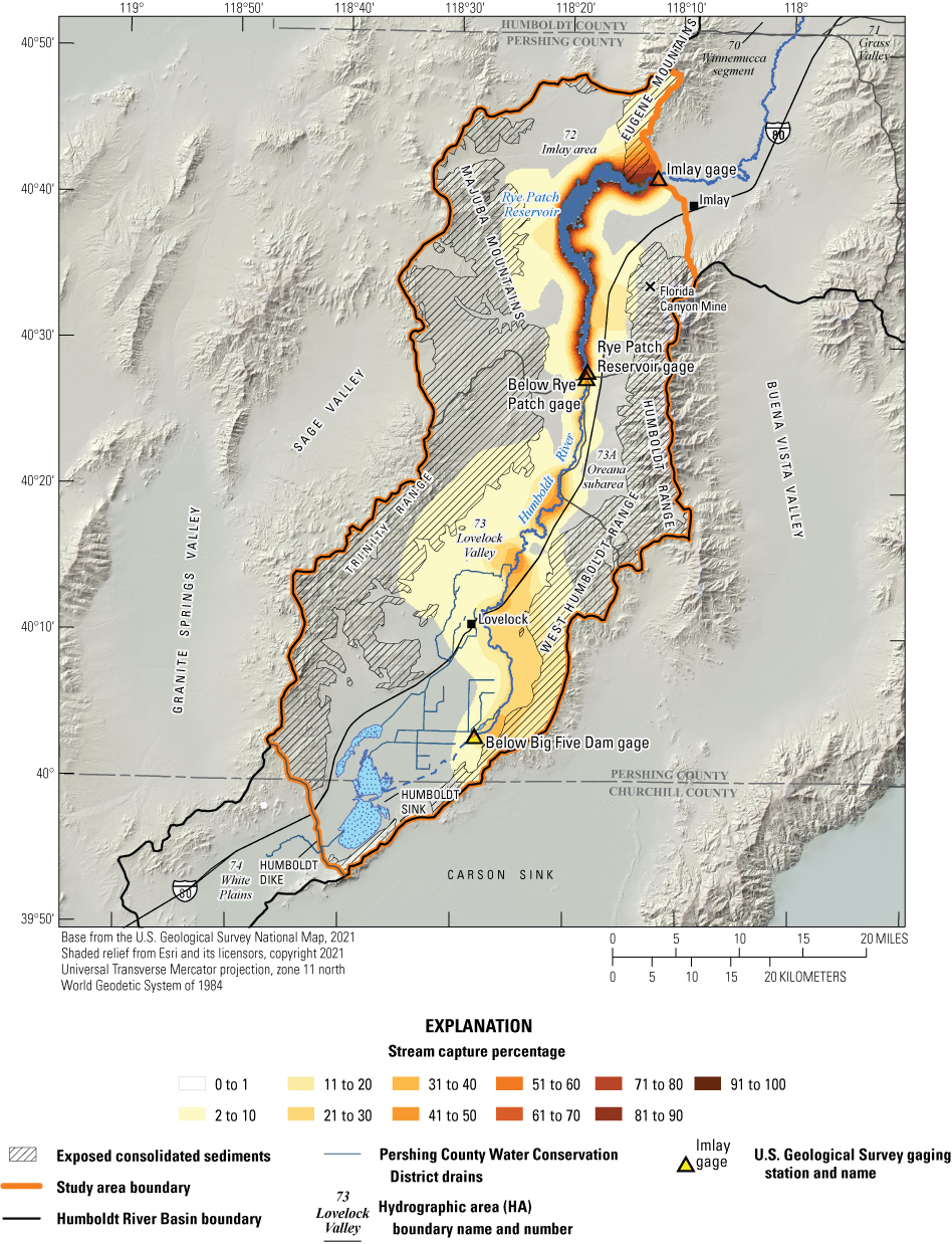
Stream capture map of layer 2 from a pumping rate of 476 acre-feet per year after 50 years of pumping.
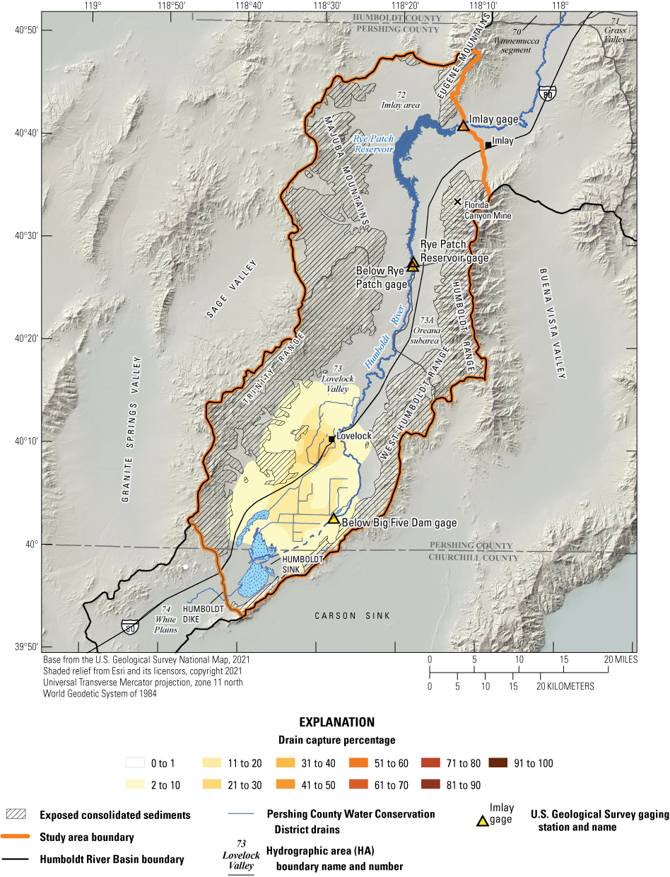
Drain capture map of layer 2 from a pumping rate of 476 acre-feet per year after 50 years of pumping.
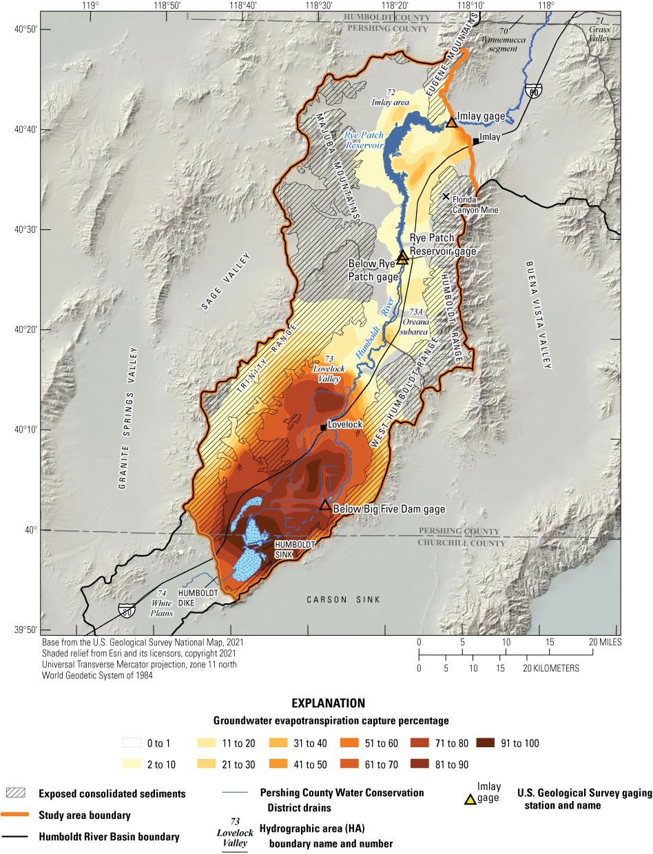
Groundwater evapotranspiration capture map of layer 2 from a pumping rate of 476 acre-feet per year after 50 years of pumping
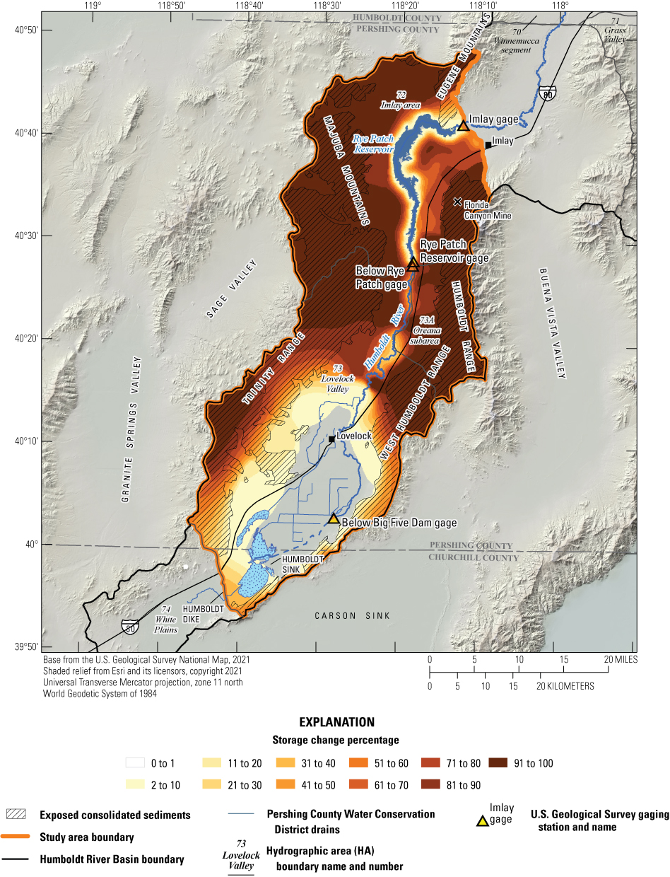
Storage change map of layer 2 from a pumping rate of 476 acre-feet per year after 50 years of pumping.
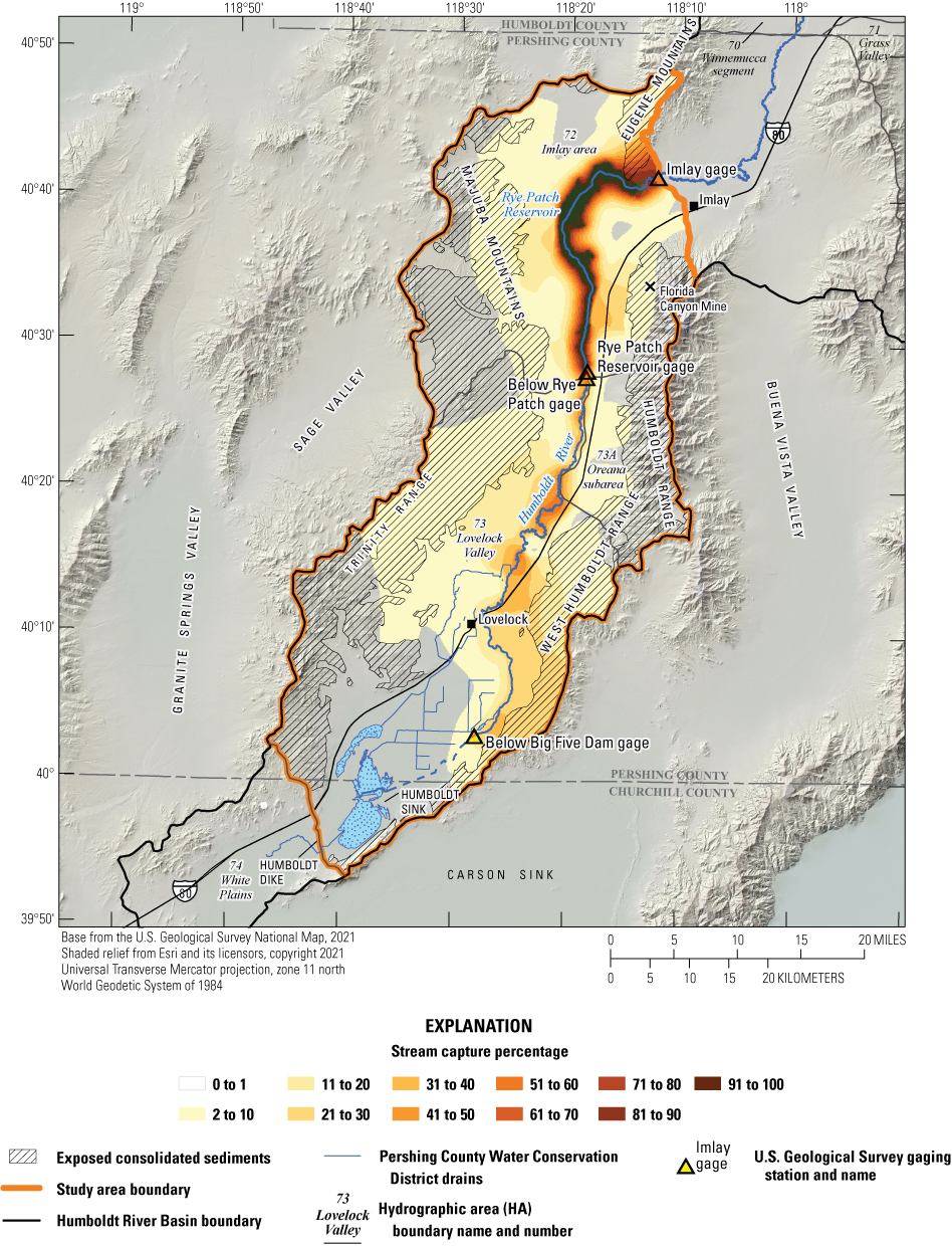
Stream capture map of layer 2 from a pumping rate of 476 acre-feet per year after 75 years of pumping.

Drain capture map of layer 2 from a pumping rate of 476 acre-feet per year after 75 years of pumping.
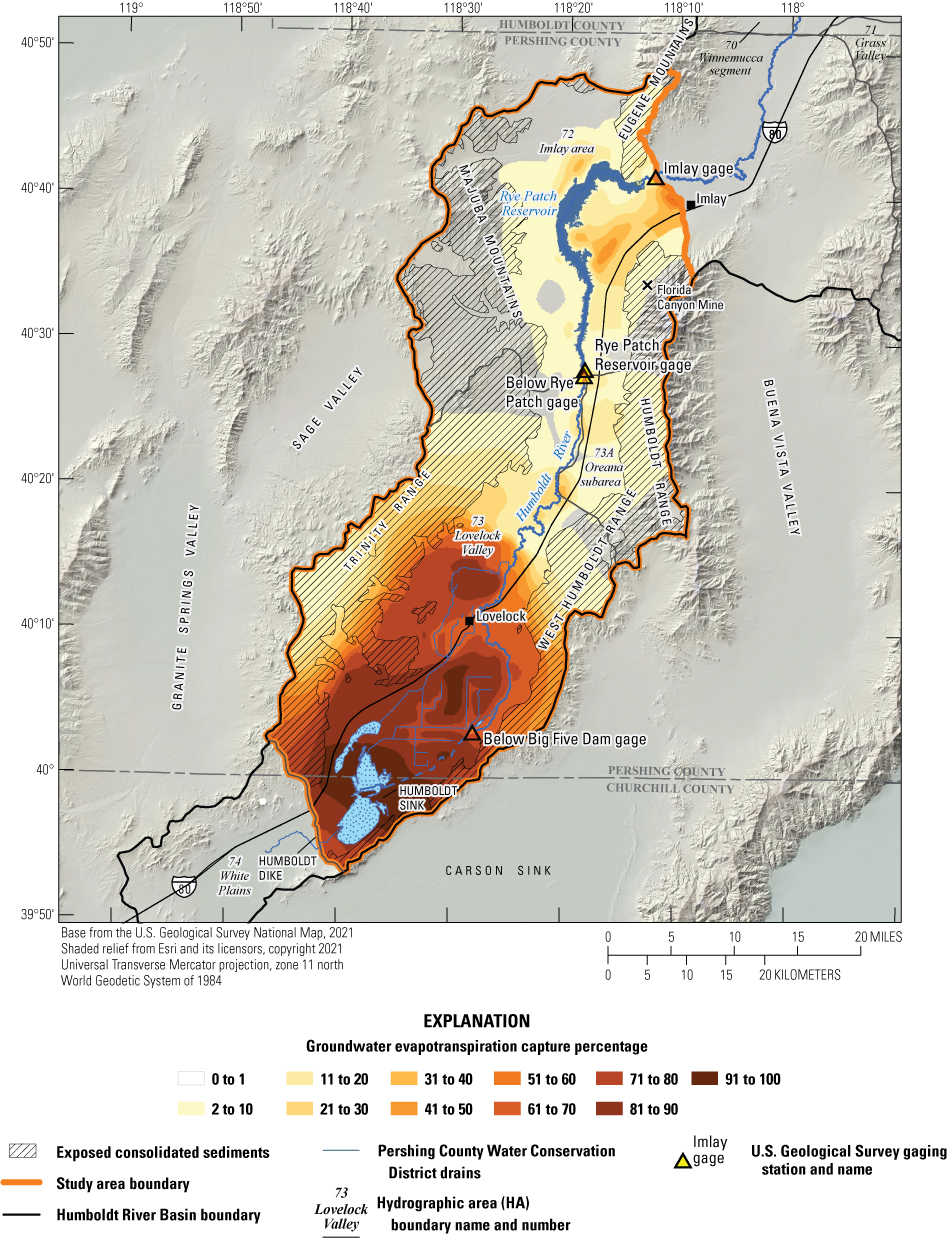
Groundwater evapotranspiration capture map of layer 2 from a pumping rate of 476 acre-feet per year after 75 years of pumping.
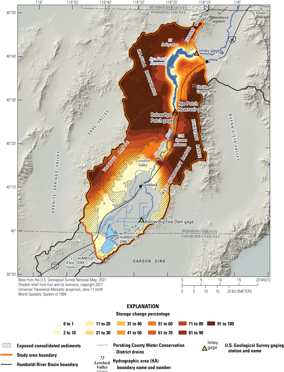
Storage change map of layer 2 from a pumping rate of 476 acre-feet per year after 75 years of pumping.

Stream capture map of layer 2 from a pumping rate of 476 acre-feet per year after 100 years of pumping.
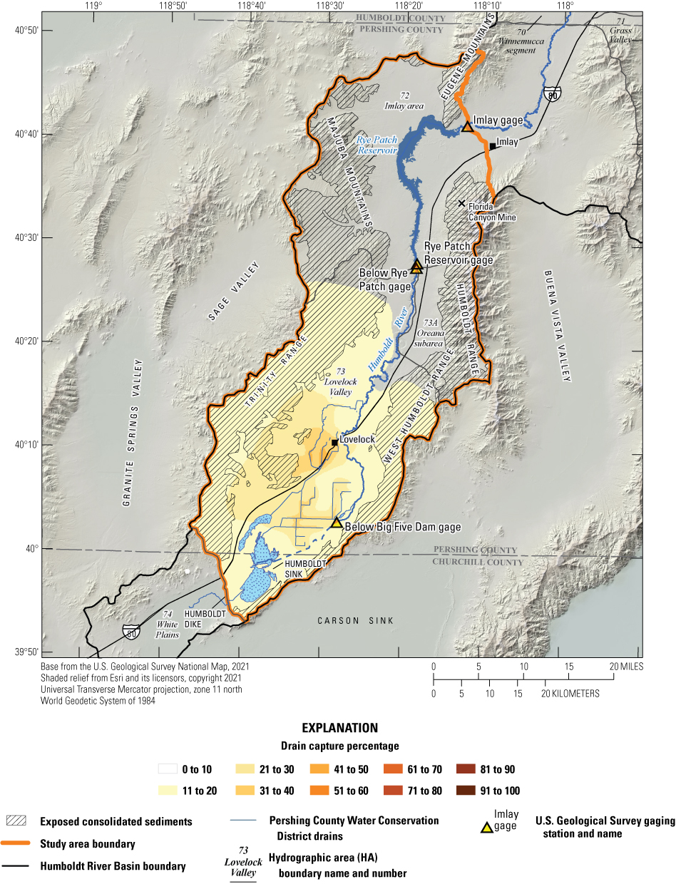
Drain capture map of layer 2 from a pumping rate of 476 acre-feet per year after 100 years of pumping.
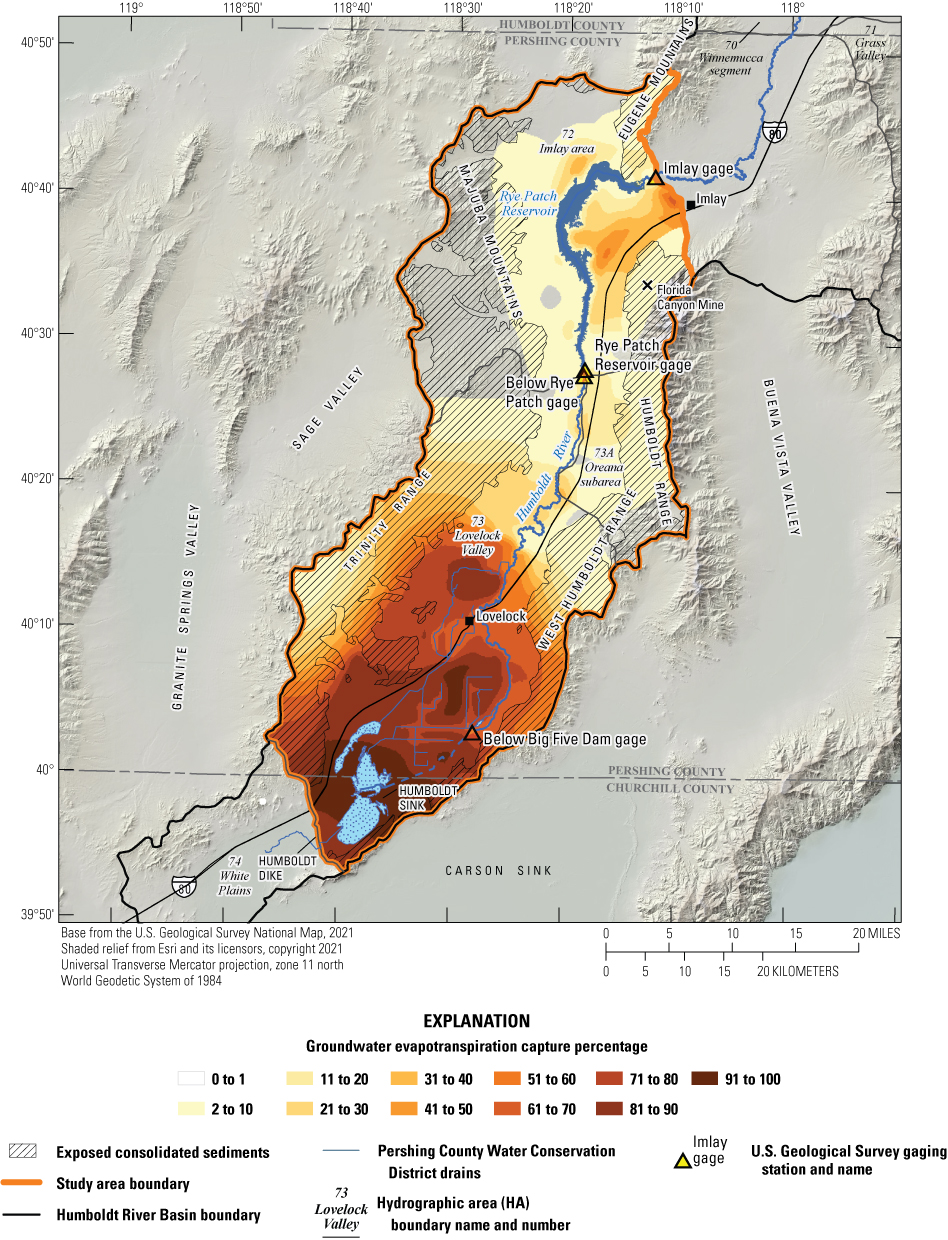
Groundwater evapotranspiration capture map of layer 2 from a pumping rate of 476 acre-feet per year after 100 years of pumping
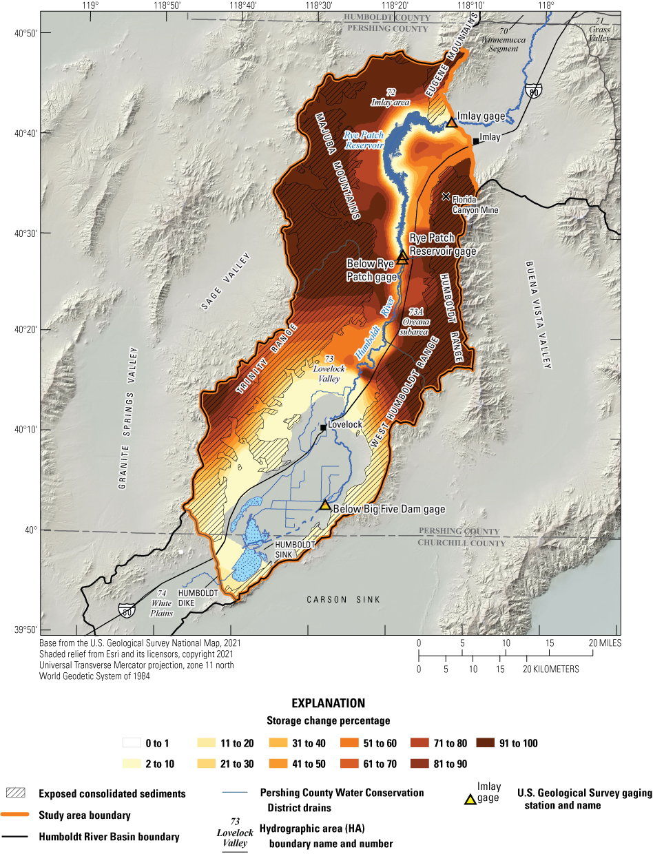
Storage change map of layer 2 from a pumping rate of 476 acre-feet per year after 100 years of pumping.
Capture percentages were calculated in each of the model’s three layers; however, only capture maps from layer 2 will be discussed in this report, except for a few small areas where hydrologic properties vary greatly, because the majority of the maps exhibit the same patterns and the majority of pumping takes place in layer 2. Although some wells are screened across more than one layer, only 6 percent (19 of 325) of the wells in the model domain are screened in the bedrock represented by layer 3. These wells are primarily domestic wells in the Oreana subarea; some are mining wells from the Florida Canyon Mine and some are domestic wells in Lovelock Valley. Layer 1 accounts for 30 percent (98 of 325) of the wells in the model domain, and layer 2 accounts for 64 percent (208 of 325) of the wells in the model domain. Capture maps, difference maps (discussed below), and statistics for each of the three layers can be recreated with the provided models, Python scripts, and explanatory text files provided in the associated model archive data release at https://doi.org/10.5066/P99DN2R1 (Nadler and others, 2023).
As previously described, capture maps are useful for visualizing potential capture effects from a well in any location and at any point in time. They can help to illustrate the effects of well placement on capture and provide a tool to better understand potential consequences of pumping an existing or new well in areas of interest within the simulated area. Regions of higher capture or storage change are represented with dark brown; regions of lower capture or storage change are represented with tan; and the color gradient in between represents values between 1 and 100 percent as shown on figures 31–50. Exposed consolidated sediment units are shown with hatching on the capture and storage change maps on figures 31–50. These units are areas with higher uncertainty, as discussed in the “Model Limitations” section, largely due to the application of recharge on these low permeability units.
Potential stream capture in the lower HRB is relatively minor, except in areas directly adjacent to the Humboldt River and Rye Patch Reservoir, where potential stream capture could be 100 percent after a period of time (figs. 31, 35, 39, 43, 47). After 1 year of pumping, potential stream capture is predicted to be zero or near-zero from pumping at nearly any location within the entire study area (fig. 31). After 10 years of pumping, potential stream capture is predicted to be zero or near-zero for all hypothetical wells except those adjacent to the Humboldt River and Rye Patch Reservoir (fig. 35). The area of potential stream capture expands outward from the Humboldt River and Rye Patch Reservoir during the 100 years of pumping (figs. 39, 43, 47). After 100 years of pumping, most wells adjacent to the Humboldt River would likely derive 50 percent of the pumped water from stream capture, whereas those adjacent to Rye Patch Reservoir have the potential to capture 100 percent of their water from stream capture (fig. 47).
Potential drain capture is a likely source for wells pumping along the drains in the Lovelock agricultural area, though this area is a very small region within the lower HRB through the first 50 years of pumping (figs. 32, 36, 40). Within a small area, potential drain capture reaches 39 percent within 50 years of pumping (fig. 40). After 50 years of pumping, the magnitude of potential drain capture remains under 40 percent. Between 50 and 100 years of pumping, the area of potential drain capture expands across the lower half of the study area (figs. 40, 44, 48). Outside of the drain network of the Lovelock agricultural area, potential drain capture is generally between 11 and 20 percent after 100 years of pumping (fig. 48).
Although potential stream and drain capture are relatively small in the lower HRB, potential ETg capture and potential storage change are much more significant. The lower HRB is dominated in the northern half of the basin by large areas wherein pumping would cause substantial storage change (figs. 34, 38, 42, 46, 50). In the southern half of the basin, there is a large area wherein pumping would source a substantial amount of water from ETg capture (figs. 33, 37, 41, 45, 49). After 1 year of pumping, potential ETg capture would be relatively low in the lower HRB except for pumping locations within the agricultural area (fig. 33). After just 1 year of pumping, nearly all pumping that may occur outside of the agricultural area would source all, or nearly all, water from storage change (fig. 34). The area of potential ETg capture would expand during 100 years (figs. 33, 37, 41, 45, 49) until the primary potential source of water to wells near Lovelock Valley would be ETg capture after 100 years of pumping (fig. 49). Only wells that would potentially be along the riparian corridor and on the east side of the Humboldt River near the City of Lovelock would source the largest percentage of water from stream capture (fig. 47). Wells outside of Lovelock Valley and not directly adjacent to the Humboldt River would potentially source all or most of their water from storage change (figs. 34, 38, 42, 46, 50).
The Florida Canyon Mine, east of Rye Patch Reservoir, was sporadically active between 1986 and 2004 and began production again in April 2017 (fig. 15; https://westernmininghistory.com/mine_detail/10310409/ and https://www.argonautgold.com/English/assets/operations/Florida-Canyon/default.aspx). A nearby fault acts as a horizontal flow barrier between the portions of the aquifer underlying the Humboldt River and surrounding the mine (fig. 14). As such, the capture analysis indicates the mine would source nearly all of its pumped water from groundwater storage for up to 100 years (figs. 34, 38, 42, 46, 50).
Capture and Storage Change Summary
As demonstrated with the capture and storage change maps shown on figures 31–50, the potential for stream capture is relatively low throughout most of the lower HRB, with the exception being from hypothetical wells directly adjacent to the Humboldt River and Rye Patch Reservoir. Another way to examine potential capture is to plot mean potential capture and storage change fractions as presented on figure 51. This graph plots the mean of the 388,362 capture and storage change fractions from all locations within the capture map area through time during 100 years of pumping. It illustrates the relative distribution and dynamics of the capturable components for the entire lower HRB though time. In effect, the plot characterizes the capture potential for the entire region, under the assumption that pumping would be evenly distributed across the entire region. As such, the capture tendency graph illustrates the propensity for the entire region to experience capture-related impacts independent of spatial bias in pumping distribution.
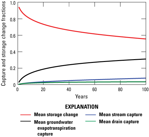
Mean potential capture and storage change fractions derived from all potential capture wells pumping at 476 acre-feet per year in layer 2.
On average, potential storage change would be the dominant source of water to wells at most locations in the lower HRB, with a potential average fraction for the region remaining over 0.55 after 100 years of pumping (fig. 51). Potential ETg capture is the second largest potential source of capture in the model domain, with average values for the region reaching 0.31 after 100 years of pumping (fig. 51). Mean potential stream and drain capture are relatively minor sources of capture in the model domain. The mean potential stream capture remains below 0.08 after 100 years of pumping, and mean potential drain capture remains below 0.04 after 100 years of pumping (fig. 51).
In the lower Humboldt River Basin, hypothetical wells in the Lovelock agricultural area would likely source the majority of pumped water from ETg capture and drain capture. Potential wells placed directly adjacent to the Humboldt River and Rye Patch Reservoir would likely source the majority of pumped water from stream capture. Potential wells placed near the existing Florida Canyon Mine would be separated from the Humboldt River and Rye Patch Reservoir by a fault that acts as a barrier to horizontal flow and would therefore source the majority of hypothetically pumped water from groundwater storage. Wells in the northern region of the lower HRB, which are far from the agricultural activity driving potential ETg and drain capture, would source a majority of water from groundwater storage and not capture.
Capture Uncertainty
The predictive accuracy of a capture map derived from a nonlinear model may be affected in regions where nonlinear flow processes contribute to greater uncertainty. The use of capture analysis methods to predict the combined effect of multiple pumping wells or pumping a single well at different rates on stream capture relies on the principle of superposition. However, the principle of superposition is mostly applicable for linear groundwater flow models (Reilly and others, 1987) and can have some limitations with use of nonlinear flow processes within models, which are needed to simulate head-dependent flow processes (such as ETg or drying streams) and unconfined aquifers (Konikow and Leake, 2014; Nadler and others, 2017). Thus, when using a capture map derived from a nonlinear groundwater flow model to estimate potential capture for multiple wells or a single well at a different rate than simulated, use of the principle of superposition may lead to somewhat greater uncertainty in the predictive capture results. The total potential capture calculated for a capture map versus the total potential capture that is calculated by simulating pumping from a set of wells or pumping a single well at a different rate may be different when determined using a nonlinear model. This difference, called capture map bias (CMB), describes the degree to which potential capture calculated for a capture map may either overestimate or underestimate true capture (Nadler and others, 2017).
Capture map uncertainty may occur when nonlinear flow processes are represented in a groundwater flow model. Nonlinear flow processes, such as ET, can cause different results derived from different pumping rates. For example, the groundwater table may lower below the root zone faster in response to pumping when a higher pumping rate is used to create a capture map.
Additionally, capture uncertainty can arise from uncertainty in parameter estimation. A covariance matrix adaptation-evolution strategy can be used to evaluate and quantify the resulting capture uncertainty due to parameter estimation.
Capture Map Uncertainty—Capture Difference Maps
Regions that are sensitive to nonlinear flow processes and that may have a greater degree of uncertainty in capture results can be assessed by differencing capture maps developed from different levels of pumping (Nadler and others, 2017). Capture difference maps are used to assess and visualize the regions of the lower HRB capture maps where greater uncertainty from nonlinear flow processes may exist. For this study, capture difference maps were developed from the difference between potential capture fractions for each active model cell, as derived from the capture map, and capture fractions derived for pumping rates that are an order of magnitude above and below the 476 acre-ft/yr pumping rate used to create the capture map. An additional 776,724 capture model runs (resulting in a total of 1,165,086 capture models) were used to calculate capture uncertainty. Half of these new model runs (388,362) included potential capture wells pumping at 48 acre-ft/yr (5,684.2 ft3/day). The remaining half of the model runs included potential capture wells pumping at 4,762 acre-ft/yr (568,420 ft3/day). Then, the potential capture and storage terms were divided by the capture pumping rate in each model run to calculate time-varying potential capture fractions across the model domain.
Capture fraction differences were determined for each active model cell by subtracting the potential capture fractions for the higher pumping rate (4,762 acre-ft/yr) from the potential capture fractions for the lower pumping rate (48 acre-ft/yr). A negative value indicates a higher potential capture fraction from a higher pumping rate and a positive value indicates a lower potential capture fraction from a higher pumping rate. Regions where capture fractions are insensitive to the magnitude of pumping rates are characterized by zero values, indicating that the potential capture fraction for that particular area is independent of pumping rate, and capture behaves in a linear manner with respect to the magnitude of pumping. The nearer to zero the capture fraction difference is, the less uncertainty there is when applying the capture map results to different pumping rates. This analysis is conducted for each component of capture and storage change and is evaluated for 1 (fig. 52) and 25 years (fig. 53) of pumping. Capture and storage change fraction differences are contoured to display spatial variability of potential capture and potential storage change fraction sensitivity to pumping rates. Results from these maps reveal regions where there is greater potential for uncertainty due to CMB related to nonlinear processes.
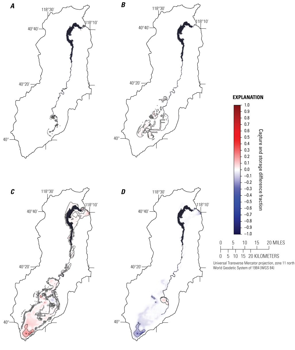
Capture and storage difference maps of layer 2 derived from pumping rates of 48 and 4,762 acre-feet per year after 1 year of pumping for potential A, stream capture; B, drain capture; C, groundwater evapotranspiration capture; and D, storage change. Capture and storage change difference contours depicted use an interval of 0.1.
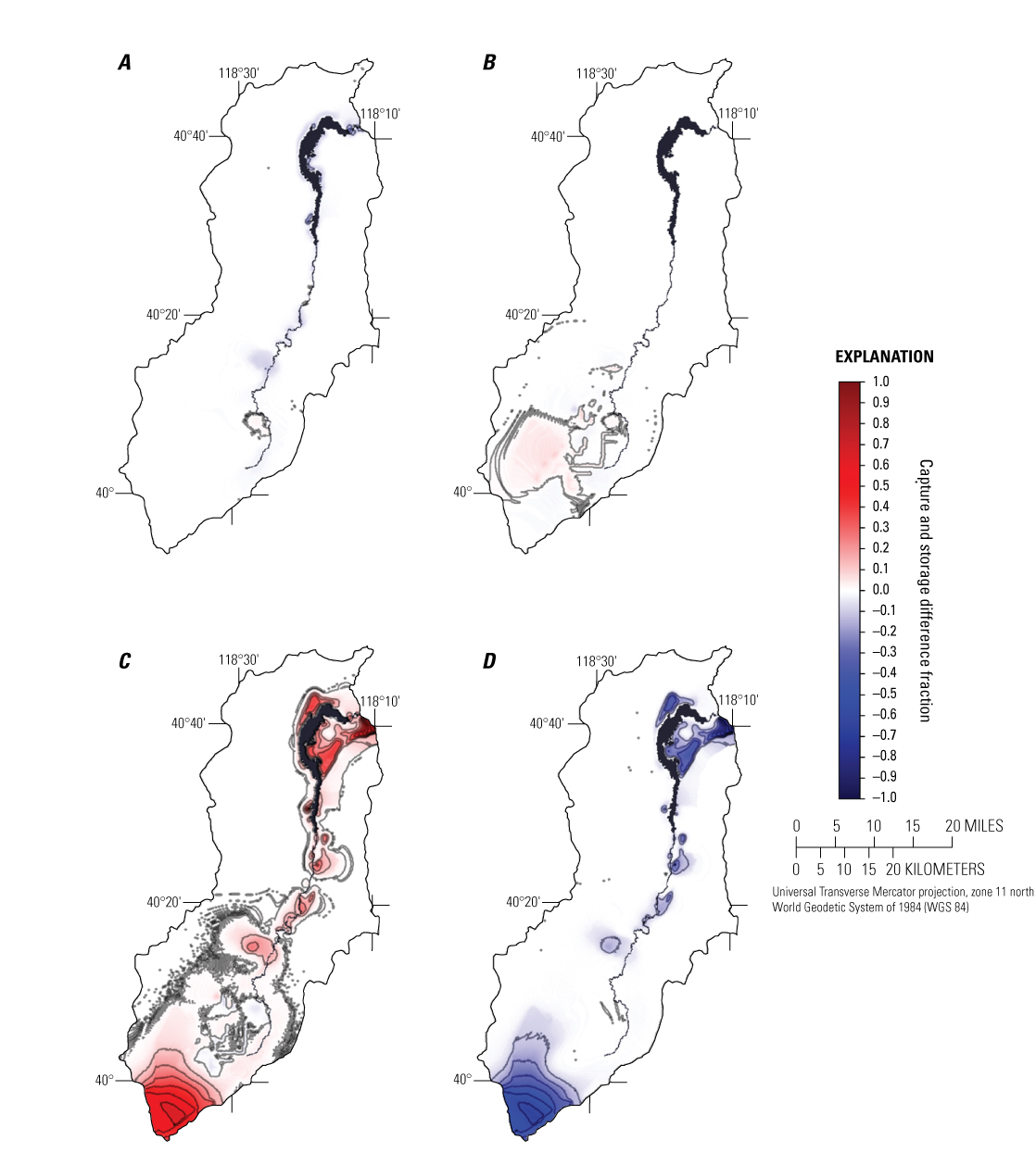
Capture and storage change difference maps of layer 2 derived from pumping rates of 48 and 4,762 acre-feet per year after 25 years of pumping for potential A, stream capture; B, drain capture; C, groundwater evapotranspiration capture; and D, storage change. Capture and storage change difference contours depicted use an interval of 0.1.
Capture Map Regions Affected by Nonlinear Flow Processes
Potential stream capture differences were generally small in the lower HRB, with small negative differences along the Humboldt River and Rye Patch Reservoir (figs. 52A, 53A). The small negative capture differences indicate that wells pumping at higher pumping rates can potentially capture a slightly greater fraction of stream water than wells pumping at lower pumping rates. The Humboldt River is represented with the MODFLOW RIV Package, and Rye Patch Reservoir is represented with the MODFLOW CHD Package. The MODFLOW RIV Package simulates the river as a head-dependent boundary condition. Although there are small areas of negative capture differences along the river, these differences are relatively insignificant. Thus, the MODFLOW RIV Package is not introducing much model nonlinearity. The MODFLOW CHD Package simulates the reservoir as constant head boundaries, meaning that water is added to those model cells when pumping occurs to maintain the same head over time. Constant head boundaries represent a consistent source of water to wells and are less sensitive to nonlinear flow processes; this is made evident by the small and relatively insignificant regions of negative capture differences along Rye Patch Reservoir.
Drain capture differences also were generally small in the lower HRB with small, positive differences in the Lovelock agricultural area (figs. 52B, 53B). Areas with positive capture fraction differences yielded lower potential capture fractions with higher pumping rates; this means wells along the drains have the potential to capture a greater proportion of ETg for a longer amount of time with a lower pumping rate. That is, the water table lowers at a slower rate with the lower pumping rate, meaning that wells in red areas on figures 52B and 53B are able to sustain drain water as a source of potential capture for longer at lower pumping rates than at higher pumping rates. Drains in the Lovelock agricultural area are represented with the MODFLOW DRN Package, which simulates a head-dependent boundary condition. Drains are connected to the water table at a specified elevation (Harbaugh and others, 2000; Harbaugh, 200517). When the water table drops below the specified elevation, the drain is essentially shut off as a source for capture. Although the MODFLOW DRN Package has the potential to introduce model nonlinearity, the degree of nonlinearity is small given the small capture fraction differences. Drains are localized solely to the Lovelock agricultural area, and therefore only contribute to a small uncertainty in that region alone.
Groundwater evapotranspiration capture differences were generally positive and significant in regions in the Lovelock agricultural area and along the Humboldt River (figs. 52C, 53C). Over time, this area of positive ETg capture differences expanded outward after 25 years of pumping and are anticipated to eventually encapsulate much of the model domain after 100 years of pumping. Areas with positive capture fraction differences yielded lower potential capture fractions at higher pumping rates; this means potential wells in Lovelock and along the Humboldt River and Rye Patch Reservoir, and eventually in much of the model domain, captured a greater proportion of ETg for a longer amount of time at a lower pumping rate than at a higher pumping rate. The simulated groundwater ETg rate varies with the position of the water table (Harbaugh, 2005). When the water table is at land surface, the maximum ETg rate is simulated; this rate linearly decreases with a declining water table until it reaches the extinction depth, at which point the ETg rate is simulated as zero, essentially shutting off ETg as a potential source of capture. Higher pumping rates lower the water table faster than the lower pumping rates and can essentially shut off these head-dependent sources of capture earlier; this discrepancy in timing is what causes the capture fraction differences. Simulated ETg, unlike drains, is a source of potential capture across much of the model domain and is therefore a primary process leading to greater uncertainty in estimated ETg.
Conversely, storage change differences were generally negative and significant in regions in the Lovelock agricultural area and along the Humboldt River and Rye Patch Reservoir (figs. 52D, 53D). Storage is readily available in the model and compensates for the capture differences caused by the head-dependent drain and ETg boundaries in the model where stream water is not readily available. The negative values indicate that the higher pumping rate resulted in a higher potential storage change fraction than the lower pumping rate did; this indicates that the capture wells in these and other regions colored blue on figures 52D and 53D depleted head-dependent boundary conditions sooner with higher pumping rates, and thus drew a greater proportion of water from storage over time.
Capture Uncertainty Due to Parameter Estimation
Capture prediction uncertainty due to parameter estimation was evaluated using the covariance matrix adaptation-evolution strategy (CMA-ES; Hansen and others, 2003; Elshall and others, 2015). The CMA-ES belongs to the class of evolutionary algorithms. In each iteration (generation), model parameter sets (new individuals) are stochastically generated by variating the current parameter sets (parental individuals). Some best individuals are then selected to become the parents in the next generation based on their objective function value (root mean square error in this study). In this way, individuals with better and better fitness values are generated over the generation sequence. The important features in the CMA-ES are global-local search capability, parallelization, and uncertainty quantification for estimated parameters, which are especially effective at calibrating computationally demanding groundwater models. The global search capability of the CMA-ES can be enhanced by increasing the population size (the number of new individuals generated in each generation). In addition to the global-local search capabilities and parallelization, another useful feature of CMA-ES is the ability to quantify model parameter uncertainty due to parameter estimation error. The solutions of the CMA-ES, which consist of a maximum likelihood estimate and a full covariance matrix of model parameters, can be used for Monte Carlo sampling.
To implement the CMA-ES for uncertainty quantification, the initial parameter values were taken from the historical transient model. These parameters included hydraulic conductivity, specific storage, river conductance, drain conductance, maximum ETg rates, and the hydraulic characteristic of the horizontal flow barrier near the Florida Canyon Mine (the hydraulic conductivity of the barrier divided by its thickness). The parameter ranges were generated by varying the initial parameter values by plus or minus (±) 80 percent. Using the maximum likelihood estimate and the covariance of model parameters estimated by CMA-ES during model calibration, 100 Monte Carlo realizations of model parameters were generated assuming a multi-Gaussian distribution. Designated as points A–M on figure 54, 13 grid cells in layer 2 were selected from the model domain to assess capture uncertainty in a variety of settings. One hundred groundwater model realizations were run to quantify capture prediction uncertainty at each of these cell locations, for a total of 1,300 model runs. Pumping for all capture wells was set to 476 acre-ft/yr (56,842 ft3/d), the value used in the capture model to develop the capture maps, and rates of recharge and background pumping were held constant at the same rates used for those simulations.
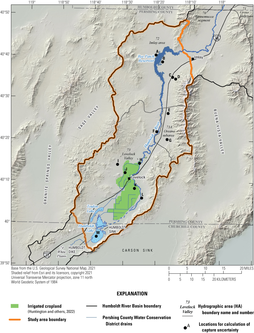
Selected locations for calculation of capture uncertainty.
Capture uncertainty curves are shown for each of the 13 grid cells on figures 55–59. At each tested location, the uncertainty in capture fraction for a given source (stream capture, drain capture, ETg capture, or storage change) at a given pumping duration can be quantified by the range of capture fractions for that source and stress period. For the 13 locations sampled, stream capture uncertainty after the 100-year pumping duration ranged from no uncertainty (±8.52E-5) at point M (fig. 59), in the Humboldt Sink where no stream capture is simulated, to ±0.168 at point B (fig. 55), adjacent to the Rye Patch Reservoir on the southwest side where a high degree of stream capture would potentially occur. Several of the northernmost points show no drain capture, so the minimum drain capture uncertainty is therefore zero. The maximum drain capture uncertainty at the 100-year stress period was fairly small at ±0.0965 at point K (fig. 58) in the Lovelock Valley agricultural area where drain capture is more of an important source of supply to wells. Groundwater evapotranspiration capture uncertainty after the 100-year pumping duration ranged from a very low ±0.030 at point E (fig. 56), at the northern end of the Oreana subarea (fig. 54) where storage would supply greater than 90 percent of a pumping well supply for up to and beyond 100 years, to ±0.195 at point K (fig. 58), in the Lovelock Valley agricultural area (fig. 54) where ETg is predicted to be a major component of a pumping wells’ water supply after just a few years of pumping. Storage change uncertainty after the 100-year pumping duration ranged from very little uncertainty (±1.34E-3) at point K (fig. 58), in the Lovelock Valley agricultural area where capture is dominated by ETg, to the broadest range in values of ±0.223 at point B (fig. 55), adjacent to the Rye Patch Reservoir on the southeast side (fig. 54) where storage would be the dominant component of supply for approximately 60 years of pumping.
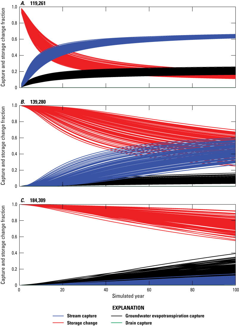
Capture and storage change uncertainty results for points in A, row 199 and column 261; B, row 139 and column 280; and C, row 184 and column 309 (fig. 54) in layer 2. Title for each plot indicates the row and column of the tested grid cell.
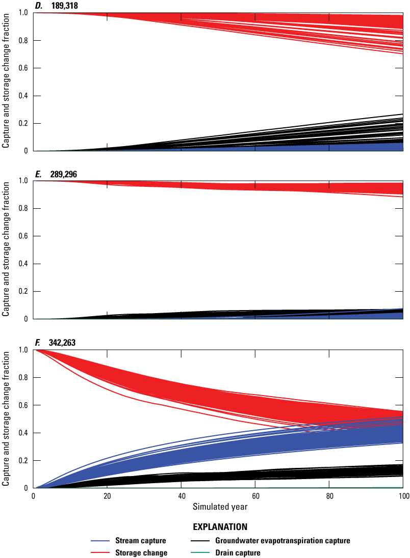
Capture and storage change uncertainty results for points in D, row 189 and column 318; E, row 289 and column 296; and F, row 342 and column 263 (fig. 54) in layer 2. Title for each plot indicates the row and column of the tested grid cell.
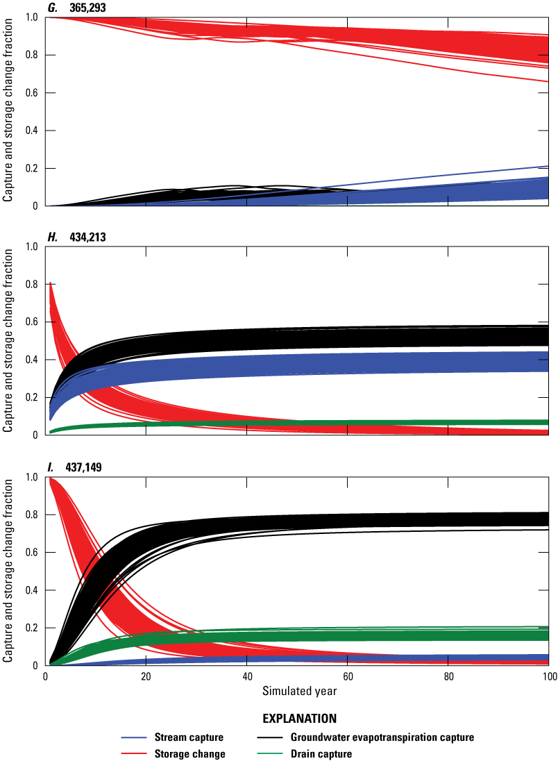
Capture and storage change uncertainty results for points in G, row 365 and column 293; H, row 434 and column 213; and I, row 437 and column 149 (fig. 54) in layer 2. Title for each plot indicates the row and column of the tested grid cell.
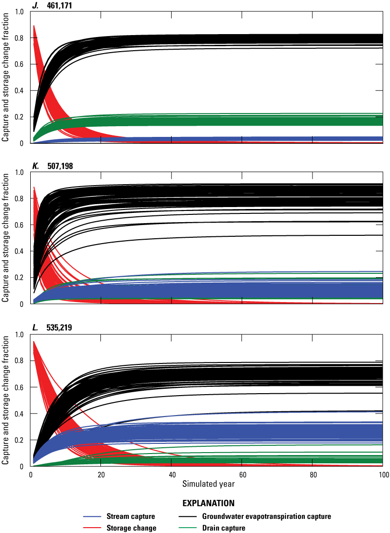
Capture and storage change uncertainty results for points in J, row 461 and column 171; K, row 507 and column 198; and L, row 535 and column 219 (fig. 54) in layer 2. Title for each plot indicates the row and column of the tested grid cell.
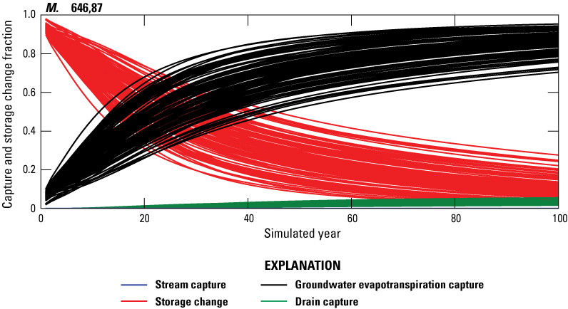
Capture and storage change uncertainty results for point in M, row 646 and column 87 (fig. 54) in layer 2. Title for the plot indicates the row and column of the tested grid cell.
In general, results indicate that poorly estimated hydraulic properties would result in greater capture uncertainty based on proximity to that source—thus capture results from pumping in cells close to the river tend to show greater sensitivity to hydraulic property estimates (as seen at points B, F, H, K, and L; figs. 55–58). Likewise, drain capture uncertainty is greatest (though still small) in the agricultural area of Lovelock Valley where the drains are, as seen at points I, J, K, and L (figs. 57–58). Interestingly, stream capture uncertainty is relatively low at point A (fig. 55), on the northwest side of Rye Patch Reservoir, although the stream capture fraction itself exceeds 0.6 after 100 years.
Capture Sensitivity to Storage Parameters
As discussed in the “Model Limitations” section, the calibrated value for specific storage in layer 2 (0.0003 ft–1) led to the hypothesis that the conceptual model of a confined aquifer may be incorrect, and that the system may actually be unconfined or leaky-confined. To test the sensitivity of stream capture to specific storage, an additional sensitivity model was run using specific storage values of 0.003 ft–1 in layer 1 and 4E-6 ft–1 in layer 2, as opposed to 0.0003 ft–1 in both layers for the calibrated model. The increase in specific storage in layer 1 was designed to represent an aquifer with a storativity of 0.15, appropriate for an unconfined aquifer, without needing to adjust the model configuration that simulated layer 1 as confined. This change was made while simultaneously reducing the specific storage in layer 2 to a value that represents the alternate conceptualization of a leaky-confined or unconfined aquifer.
Aside from the specific storage values assigned to layers 1 and 2, all other model parameters remained unchanged from the calibration model. A comparison of simulated and observed heads for the calibrated model and sensitivity model for three wells (one each from the Imlay area, Oreana subarea, and Lovelock Valley) is shown on figures 60A–C. This analysis was done to ensure that the sensitivity model could serve as a reasonable alternate representation of reality, and that any differences in stream capture between the calibration and sensitivity models were primarily a function of the differences in storage properties rather than a drastic difference in the simulated hydrologic system. Results indicate that simulated heads from both the calibration and sensitivity models reasonably represent the trends of observed heads (figs. 60A–C).
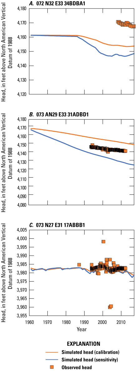
Simulated and observed heads for the calibrated model and the sensitivity model at wells located in A, the Imlay area, B, the Oreana subarea, and C, Lovelock Valley.
Stream capture results for the calibrated model and the sensitivity model are compared on figure 61. Fluctuations in total stream capture occur contemporaneously with increases in pumping in the historical period for each of the two models, though capture is higher in the sensitivity model. During the predictive period, predictive stream capture increases slowly, reaching a fraction of 15.3 percent (443 acre-ft/yr) in 2116 in the sensitivity model, compared to 8.7 percent (253 acre-ft/yr) in the calibrated model.
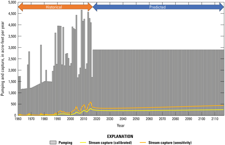
Pumping and stream capture rates for the transient historical period (1960–2016, below the orange arrow) and a 100-year predictive period (2017–2116, below the blue arrow). The yellow and orange lines represent net stream capture from the Humboldt River and Rye Patch Reservoir for the calibration and sensitivity models, respectively.
Summary
Three concurrent studies in the Humboldt River Basin (HRB) have been conducted to estimate the effects of groundwater pumping on Humboldt River flow. The three studies were broken out by location: (1) the upper HRB, (2) the middle HRB, and (3) the lower HRB. This report summarizes the work completed for the lower HRB. The objective of this study was to estimate capture and storage change caused by groundwater withdrawals in the lower HRB and to provide the Nevada State Engineer with tools needed to manage groundwater and surface-water resources.
Numerical groundwater flow models were developed for the purpose of estimating historical stream capture from pre-2016 pumping, predictive stream capture caused by predicted future pumping, and potential stream capture that could be caused by hypothetical pumping at any location within the lower HRB. These models were developed using MODFLOW-NWT to represent components of the lower HRB hydrologic system, including the Humboldt River; Rye Patch Reservoir; evapotranspiration (ET); pumping from municipal, agricultural, mining, and domestic wells; and agricultural drains. Aquifer properties were estimated using results from numerous single- and multi-well aquifer tests (Nadler, 2020) and through the process of model calibration.
Historical capture was estimated for 1960–2016, and predictive capture for the system was projected 100 years into the future (2017–2116) based on historical pumping patterns. Stream capture and drain capture were relatively low for the historical and predictive periods. During the historical period, increased pumping during dry years resulted in decreased storage change because drawdown expanded farther from the wells to capture discharge from other sources. Depleted aquifer storage has historically been replenished during wet years when groundwater levels recover. Overall, storage change has been the main source of water to wells in the lower HRB, followed by groundwater evapotranspiration (ETg) capture. If pumping continues during the predictive period, 9 percent of the water pumped would be sourced from streams after 100 years.
Capture and storage change maps were created for the lower HRB as tools that can be used to visualize spatial variability in potential capture and storage change through time and to provide a database of results that can be used to conjunctively manage groundwater and surface-water resources. These maps show that stream capture is a minor source of water for existing or potential wells located across the majority of the study area, except in areas where a well is adjacent to the Humboldt River or Rye Patch Reservoir. Hypothetical wells directly adjacent to the Humboldt River would likely derive 50 percent of the pumped water from stream capture, and wells directly adjacent to Rye Patch Reservoir would likely capture 100 percent of their water from stream capture within 100 years of pumping. Drains also are likely a minor source of water to hypothetical wells except for those directly adjacent to the drains, where potential drain capture reaches 39 percent within 50 years of pumping. In general, new wells would likely be supplied by groundwater storage in the near term and increasingly supplied by ETg in the long-term, particularly in the agricultural area. In the majority of the study area, hypothetical wells would source nearly 100 percent of pumped water from storage after 1 year of pumping. Hypothetical wells in the agricultural region of Lovelock Valley would source 70 percent or more of pumped water from ETg capture after 50 years of pumping.
Capture difference maps were generated to visualize where capture results might have larger uncertainty associated with nonlinear flow processes. Stream capture differences are highest directly adjacent to the river but are otherwise minimal. Drain capture differences are highest in the region of the drains but are otherwise minimal. The river, reservoir, and drains introduce very little nonlinearity to the model, and their associated capture map biases (CMB) are relatively minimal. Groundwater ET capture introduces nonlinearity to the model that has the potential to result in large, localized ETg CMB over time. Groundwater evapotranspiration capture differences are the result of higher pumping rates lowering the water table below the phreatophyte root extinction depth faster than lower pumping rates and essentially removing ETg as a potential source of capture faster than for lower pumping rates. Wells that can no longer source their supply through the capture of ETg begin to source more of their water from groundwater storage. Thus, potential storage change bias offsets ETg capture bias, increasing over time as well.
Capture prediction uncertainty due to parameter estimation was evaluated using a covariance matrix adaptation-evolution strategy (CMA-ES). One hundred Monte Carlo realizations of model parameters were applied to the model to assess capture uncertainty at 13 locations within the model domain. Results indicated that greater capture uncertainty for a given source (river, drains, or ET) is associated with proximity of a well to that source. After 100 years, the magnitude of maximum capture fraction uncertainties for stream capture, drain capture, ETg capture, and storage change were plus or minus (±) 0.17 ±0.10, ±0.20, and ±0.22, respectively.
References Cited
Barlow, P.M., and Leake, S.A., 2012, Streamflow depletion by wells—Understanding and managing the effects of groundwater pumping on streamflow: U.S. Geological Survey Circular 1376, 84 p. [Available at https://doi.org/10.3133/cir1376.]
Breazeale, D., and Owens, M., 2000, Pershing County agricultural statistics (2000–2001): Lovelock, Nev., Nevada Agricultural Statistics Service. [Available at https://extension.unr.edu/publication.aspx?PubID=2414.]
Bredehoeft, J.D., Papadopulos, S.S., and Cooper, H.H., Jr., 1982, Groundwater—The water-budget myth in Scientific basis of water-resource management—Studies in geophysics: Washington, D.C., National Academy Press, p. 51–57. [Available at http://water.nv.gov/hearings/past/Spring%20-%20Cave%20-%20Dry%20Lake%20and%20Delamar%20Valleys%202011/Exhibits/Utah%20Counties%20Exhibits/MILL_Exh_014 %20Bredehoeft_et_al_%20Groundwater%20-%20The%20Water%20Budget%20Myth%201982.pdf.]
Cosgrove, D.M., and Johnson, G.S., 2005, Aquifer management zones based on simulated surface-water response functions: Journal of Water Resources Planning and Management, v. 131, no. 2, p. 89–100. [Available at https://doi.org/10.1061/(ASCE)0733-9496(2005)131:2(89).]
Davids, J.C., and Mehl, S.W., 2014, Sustainable capture—Concepts for managing stream-aquifer systems: Groundwater, v. 53, no. 6, p. 851–858. [Available at https://doi.org/10.1111/gwat.12297.]
Doherty, J.E., and Hunt, R.J., 2010, Approaches to highly parameterized inversion—A guide to using PEST for groundwater-model calibration: U.S. Geological Survey Scientific Investigations Report 2010–5169, 37 p. [Available at https://doi.org/10.3133/sir20105169.]
Eakin, T.E., 1962, Ground-water appraisal of the Imlay area, Humboldt River Basin, Pershing County, Nevada: Nevada Department of Conservation and Natural Resources, Ground-Water Resources, Reconnaissance Series Report 5, 54 p. [Available at http://images.water.nv.gov/images/publications/recon%20reports/rpt5-imlay.pdf.]
Eakin, T.E., and Lamke, R.D., 1966, Hydrologic reconnaissance of the Humboldt River Basin, Nevada: Nevada Department of Conservation and Natural Resources, Water Resources Bulletin 32, 107 p. [Available at http://images.water.nv.gov/images/publications/water%20resources%20bulletins/Bulletin32.pdf.]
Elshall, A.S., Pham, H.V., Tsai, F.T.-C., Yan, L., and Ye, M., 2015, Parallel inverse modeling and uncertainty quantification for computationally demanding groundwater-flow models using covariance matrix adaptation: Journal of Hydrologic Engineering, v. 20, no. 8, p. 04014087. [Available at https://doi.org/10.1061/(ASCE)HE.1943-5584.0001126.]
Everett, D.E., and Rush, F.E., 1965, Water resources appraisal of Lovelock Valley, Pershing County, Nevada: Nevada Department of Conservation and Natural Resources, Water Resources Reconnaissance Series Report 32, 51 p. [Available at http://images.water.nv.gov/images/publications/recon%20reports/rpt32-lovelock_valley.pdf.]
Fereday, W., and Nash, N., 2017, Rye Patch Reservoir water budget and bank storage, Nevada: Water Resources Association 2017 Annual Conference, Reno, Nev., February 13–17, 2017. [Available at https://www.researchgate.net/publication/313838100_Rye_Patch_Reservoir_Water_Budget_and_Bank_Storage.]
Gesch, D.B., Oimoen, M.J., Greenlee, S.K., Nelson, C.A., Steuck, M.J., and Tyler, D.J., 2002, The national elevation data set—Photogrammetric engineering and remote sensing: American Society for Photogrammetry and Remote Sensing, v. 68, no. 1, p. 5–11. [Available at https://pubs.er.usgs.gov/publication/70156331.]
Hansen, N., Müller, S.D., and Koumoutsakos, P., 2003, Reducing the time complexity of the derandomized evolution strategy with covariance matrix adaptation (CMA-ES): Evolutionary Computation, v. 11, no. 1, p. 1–18. [Available at https://doi.org/10.1162/106365603321828970.]
Harbaugh, A.W., 2005, MODFLOW-2005—The U.S. Geological Survey modular ground-water model—The ground-water flow process: U.S. Geological Survey Techniques and Methods, book 6, chap. A16. [Available at https://doi.org/10.3133/tm6A16.]
Harbaugh, A.W., Banta, E.R., Hill, M.C., and McDonald, M.G., 2000, MODFLOW-2000, The U.S. Geological Survey modular ground-water model—User guide to modularization concepts and the ground-water flow process: U.S. Geological Survey Open-File Report 00–92, 121 p. [Available at https://doi.org/10.3133/ofr200092.]
Huntington, J.L., Bromley, M., Morton, C.G., and Minor, T., 2018, Remote sensing estimates of evapotranspiration from irrigated agriculture, northwestern Nevada and northeastern California: Desert Research Institute, Division of Hydrologic Sciences Publication no. 41275, 38 p. [Available at https://s3-us-west-2.amazonaws.com/webfiles.dri.edu/Huntington/Huntington_et_al_2018_-_DRI_41275.pdf.]
Huntington, J.L., Bromley, M., Minor, B., Morton, C.G., and Smith, G., 2022, Groundwater discharge from phreatophyte vegetation, Humboldt River Basin, Nevada: Desert Research Institute, Division of Hydrologic Sciences, Publication no. 41288, 156 p., accessed December 8, 2022, at https://s3-us-west-2.amazonaws.com/webfiles.dri.edu/Huntington/41288%20-%20Humboldt_ET_Final_Report.pdf.
Konikow, L.F., and Leake, S.A., 2014, Depletion and capture—Revisiting “the source of water derived from wells”: Groundwater, v. 52, no. S1, p. 100–111, accessed March 11, 2017, at https://doi.org/10.1111/gwat.12204.
Leake, S.A., Pool, D.R., and Leenhouts, J.M., 2008, Simulated effects of ground-water withdrawals and artificial recharge on discharge to streams, springs, and riparian vegetation in the Sierra Vista subwatershed of the upper San Pedro Basin, southeastern Arizona: U.S. Geological Survey Scientific Investigations Report 2008–5207, 15 p. [Available at https://doi.org/10.3133/sir20085207.]
Leake, S.A., Reeves, H.W., and Dickinson, J.E., 2010, A new capture fraction method to map how pumpage affects surface water flow: Groundwater, v. 48, no. 5, p. 690–700. [Available at https://doi.org/10.1111/j.1745-6584.2010.00701.x.]
Maurer, D.K., Lopes, T.J., Medina, R.L., and Smith, J.L., 2004, Hydrogeology and hydrologic landscape regions of Nevada: U.S. Geological Survey Scientific Investigations Report 2004–5131, 41 p. [Available at https://doi.org/10.3133/sir20045131.]
Nadler, C.A., 2016, Evaluation of capture analysis bias associated with use of nonlinear groundwater flow models: Reno, Nev., University of Nevada, Reno, M.S. Thesis, 107 p., accessed February 16, 2017, at https://scholarworks.unr.edu//handle/11714/2234.
Nadler, C.A., 2020, Analysis of aquifer framework and hydraulic properties of Lovelock Valley, Lovelock, Nevada: U.S. Geological Survey Open-File Report 2019–1133, 48 p., accessed July 21, 2021, at https://doi.org/10.3133/ofr20191133.
Nadler, C.A., Allander, K., Pohll, G., Morway, E., Naranjo, R., and Huntington, J., 2017, Evaluation of bias associated with capture maps derived from nonlinear groundwater flow models: Groundwater, v. 56, no. 3, p. 458–469. [Available at https://doi.org/10.1111/gwat.12597.]
Nadler, C.A., Rybarski, S.C., and Pham, H., 2023, MODFLOW-NWT model and supplementary data used to characterize effects of pumping in Lovelock Valley, Nevada: U.S. Geological Survey data release. [Available at https://doi.org/10.5066/P99DN2R1.]
Nevada Division of Water Resources, 2018, Water use and availability database: Nevada Division of Water Resources, accessed May 25, 2018, at http://water.nv.gov/WaterLevelData.aspx.
Niswonger, R.G., Panday, S., and Ibaraki, M., 2011, MODFLOW-NWT, A Newton formulation for MODFLOW-2005: U.S. Geological Survey Techniques and Methods, book 6, chap. A37, 44 p. [Available at https://pubs.usgs.gov/tm/tm6a37/pdf/tm6a37.pdf.]
Peterson, S.M., Stanton, J.S., Saunders, A.T., and Bradley, J.R., 2008, Simulation of ground-water flow and effects of ground-water irrigation on base flow in the Elkhorn and Loup River Basins, Nebraska: U.S. Geological Survey Scientific Investigations Report 2008–5143, 66 p. [Available at https://doi.org/10.3133/sir20085143.]
Ponce, D.A., and Damar, N.A., 2017, Depth to pre-Cenozoic bedrock in northern Nevada: U.S. Geological Survey data release, accessed September 11, 2018, at https://doi.org/10.5066/F75B01DD.
Prudic, D.E., Niswonger, R.G., and Plume, R.W., 2006, Trends in streamflow on the Humboldt River between Elko and Imlay, Nevada, 2005–5199: U.S. Geological Survey Scientific Investigations Report 2005-5199, 58 p. [Available at https://pubs.usgs.gov/sir/2005/5199/PDF/SIR2005_5199.pdf.]
Reilly, T.E., Franke, O.L., and Bennett, G.D., 1987, The principle of superposition and its application in ground-water hydraulics: U.S. Geological Survey Techniques of Water-Resources Investigations 03-B6, 28 p., accessed November 25, 2017, at https://doi.org/10.3133/twri03B6.
Robinson, T.W., and Fredericks, J.C., 1946, Ground water in Lovelock Valley, Nevada: U.S. Geological Survey, Water Resources Bulletin no. 2, 25 p. [Available at http://images.water.nv.gov/images/publications/water%20resources%20bulletins/Bulletin2.pdf.]
State of Nevada Division of Water Resources, 2018, Water use and availability—Pumpage inventories website: State of Nevada Division of Water Resources, accessed August 12, 2018, at http://water.nv.gov/PumpageInventoryFiles.aspx.
State of Nevada Division of Water Resources, 2021, Water law overview website: State of Nevada Division of Water Resources, accessed October 4, 2021, at http://water.nv.gov/waterlaw.aspx.
U.S. Geological Survey, 2018, National Water Information System—USGS water data for the nation website: U.S. Geological Survey, accessed May 29, 2018, at https://waterdata.usgs.gov/nwis/.
Glossary of Terminology
Capture Terms
capture
A reduction in discharge from the aquifer, an increase in recharge to the aquifer, or both caused by groundwater pumping. The capture components generally consist of stream capture, groundwater evapotranspiration capture, and occasionally drain capture.
capture analysis
The analysis performed to estimate capture caused by pumping. This is often done by differencing a calibrated groundwater flow model ran with pumping and without pumping to evaluate the difference in boundary fluxes caused by pumping well(s). The resulting difference in boundary fluxes, which is the capture, may be presented in volumetric rate terms or as a percentage or fraction of the simulated pumping rate.
capture curve
A graph presenting components of capture (stream capture, evapotranspiration capture, and drain capture, when applicable) plotted through time. Typically, capture curves are plotted with storage change through time as a complementary curve to represent all sources of water to a well.
capture difference maps
Capture difference maps display capture fraction differences, typically expressed as a percentage or fraction, at any given location for a given duration of pumping for a particular source of capture. Capture difference maps may be presented for various sources of capture and are named for the source. For example, a stream capture difference maps depict the difference between two stream capture fractions resulting from two different pumping rates at a given time.
capture fraction differences
The difference between potential capture fractions generated in the same model cell after the same amount of time from two different pumping rates. This analysis is conducted to evaluate spatiotemporal potential for capture map bias, or uncertainty, related to nonlinear processes such as groundwater evapotranspiration. Capture fraction differences are sometimes illustrated over an entire model domain with capture difference maps.
capture map
Capture maps display the potential capture, typically expressed as a percentage or fraction of pumping, at any given location for a given duration of pumping. Capture maps may be presented for various sources of capture and are named for the source. For example, stream capture maps depict potential stream capture, and groundwater evapotranspiration capture maps depict potential groundwater evapotranspiration capture. Global capture maps show all components of capture combined.
drain capture
A reduction in agricultural drain flow caused by pumping. Drain capture occurs as reduced discharge from the groundwater system. Drain capture also may be called drain depletion.
groundwater evapotranspiration capture (ETg capture)
A reduction in groundwater evapotranspiration as a result of groundwater level declines caused by pumping. Groundwater evapotranspiration capture also may be called captured groundwater evapotranspiration, groundwater evapotranspiration depletion, salvaged ETg, or evapotranspiration (ET) capture.
historical capture
The estimated capture that has occurred through time based on historical pumping and other historical data. This estimate is derived from the capture analysis conducted with the historical model.
potential capture
The capture that would occur through time caused by hypothetical pumping at a given location or locations. This estimate is derived from a capture analysis using a calibrated transient model having steady background stresses to produce either capture curves or capture maps. This kind of analysis is used to describe the hypothetical or potential capture that may be caused by pumping at a given location during a specified period of time. Potential capture also is referred to or discussed as hypothetical capture.
predictive capture
The estimated capture that may occur for a specified period of time into the future that is based on an assumed reasonable forecast of future pumping and distribution. This estimate is derived from capture analysis conducted with the predictive model which extends into the future. Predictive capture is often shown as an extension of the historical capture.
storage change
A reduction in groundwater storage caused by pumping. Groundwater storage is the first source of water to a well. Once a well’s cone of depression has extended far enough to reach an external source of water, the well will begin to capture from that external source and derive less of its water from groundwater storage. This term also is commonly referred to as storage depletion. Storage change is not technically capture; rather, it is complimentary to capture such that total storage change plus total capture are equivalent to the total pumping rate.
stream capture
A reduction in streamflow, either via induced recharge or reduced discharge to a stream, caused by pumping. Stream capture also is frequently referred to as streamflow depletion. Stream capture includes capture from all surface-water resources including springs, lakes, reservoirs, canals, drains, etc. The lower Humboldt River Basin (HRB) report combines Humboldt River and Rye Patch Reservoir capture into a single term (stream capture). The lower HRB report separates out drain capture into its own term to distinguish this capture from stream capture.
Model Terms
calibration model
The model used to estimate hydraulic properties of the aquifer systems based on a process of systematically adjusting model parameters to minimize the difference between simulated and physical observations. The historical, predictive, and capture models are all based on the structure and hydraulic properties from this model.
capture model
A calibrated groundwater flow model used to determine potential capture. Typically, specified fluxes in capture models are held constant for the entire simulation period, as is the case for this study.
historical model
A calibrated groundwater flow model used to estimate or summarize historical conditions and historical capture. The historical model is often the final calibration model, as is the case for this study.
predictive model
The model used to estimate predictive capture for an existing or assumed future pumping distribution. This model is based on the calibration model and projects the existing pumping distribution and stresses for some amount of time into the future.
Evapotranspiration Terms
groundwater evapotranspiration (ETg)
Discharge from the groundwater system through evaporation and transpiration processes, typically through phreatophytic and riparian vegetation and bare soil evaporation.
phreatophytic vegetation
Vegetation that sources its water from groundwater. Also, commonly referred to as Phreatophytes.
riparian vegetation
Vegetation that exists along streams and springs that is dependent on a surface water to supply the groundwater. Riparian vegetation is a special type of phreatophyte in which ETg cannot be captured without also capturing stream or spring flows.
Conversion Factors
U.S. customary units to International System of Units
Datum
Vertical coordinate information is referenced to the North American Vertical Datum of 1988 (NAVD 88). Horizontal coordinate information is referenced to the World Geodetic System of 1984 (WGS 84).
Altitude, as used in this report, refers to distance above the vertical datum.
Abbreviations
±
plus or minus
CHD
Time-Varying Constant Head Package
CMA-ES
covariance matrix adaptation-evolution strategy
CMB
capture map bias
DEM
digital elevation model
DRN
Drain Package
ET
evapotranspiration
ETg
groundwater evapotranspiration
EVT
Evapotranspiration Package
ft–1
per foot
GMS
Groundwater Modeling System
HA
hydrographic area
HFB6
Horizontal Flow Barrier Package
HRB
Humboldt River Basin
LMWD
Lovelock Meadows Water District
METRIC
Mapping EvapoTranspiration at high Resolution with Internalized Calibration
RCH
Recharge Package
RIV
River Package
USGS
U.S. Geological Survey
WEL
Well Package
For more information concerning the research in this report, contact the
Nevada Water Science Center
U.S. Geological Survey
2730 N. Deer Run Road, Suite 3
Carson City, Nevada 89701
https://www.usgs.gov/centers/nv-water
Publishing support provided by the U.S. Geological Survey
Science Publishing Network, Sacramento Publishing Service Center
Disclaimers
Any use of trade, firm, or product names is for descriptive purposes only and does not imply endorsement by the U.S. Government.
Although this information product, for the most part, is in the public domain, it also may contain copyrighted materials as noted in the text. Permission to reproduce copyrighted items must be secured from the copyright owner.
Suggested Citation
Nadler, C.A., Rybarski, S.C., and Pham, H., 2023, Evaluation of stream capture related to groundwater pumping, Lower Humboldt River Basin, Nevada: U.S. Geological Survey Scientific Investigations Report 2023–5110, 77 p., https://doi.org/10.3133/sir20235110.
ISSN: 2328-0328 (online)
Study Area
| Publication type | Report |
|---|---|
| Publication Subtype | USGS Numbered Series |
| Title | Evaluation of stream capture related to groundwater pumping, Lower Humboldt River Basin, Nevada |
| Series title | Scientific Investigations Report |
| Series number | 2023-5110 |
| DOI | 10.3133/sir20235110 |
| Publication Date | December 29, 2023 |
| Year Published | 2023 |
| Language | English |
| Publisher | U.S. Geological Survey |
| Publisher location | Reston, VA |
| Contributing office(s) | Nevada Water Science Center |
| Description | Report: x, 77 p.; Data Release |
| Country | United States |
| State | Nevada |
| Other Geospatial | Lower Humboldt River Basin |
| Online Only (Y/N) | Y |