Magnitude and frequency of floods in the Coastal Plain region of Louisiana, 2016

Paul A. Ensminger; Daniel M. Wagner; Amanda Whaling

doi:10.3133/sir20245031

Magnitude and Frequency of Floods in the Coastal Plain Region of Louisiana, 2016

Scientific Investigations Report 2024-5031

Prepared in cooperation with the Louisiana Department of Transportation and Development

By: Paul A. Ensminger, Daniel M. Wagner, and Amanda Whaling

https://doi.org/10.3133/sir20245031

Links

Document: Report (2.41 MB pdf) , HTML , XML
Data Releases:
- USGS water data for the Nation - U.S. Geological Survey National Water Information System database
- USGS data release - Flood-frequency of rural, non-tidal streams in Louisiana and part of Arkansas, Mississippi, and Texas, 1877–2016
Download citation as: RIS | Dublin Core

Acknowledgments

The authors would like to thank Kyle Green and Brian Breaker, U.S. Army Corps of Engineers, Little Rock District, for generating basin and climatic characteristics for streamgages in Louisiana.

Abstract

To improve flood-frequency estimates for rural streams in the Coastal Plain region of Louisiana, generalized least-squares regression techniques were used to relate corresponding annual exceedance probability streamflows for 211 streamgages in the region to a suite of explanatory variables that include physical, climatic, pedologic, and land-use characteristics of the streamgage drainage area. The resulting generalized least-squares models can be used to estimate selected annual exceedance probability streamflows for rural ungaged locations in the Coastal Plain region of Louisiana. For the 211 streamgages in the Coastal Plain region of Louisiana and surrounding States, annual peak-streamflow data available through the 2016 water year were used in this study. Two unique flood regions, the Mississippi Alluvial Plain and Coastal Plain, were identified as separate hydrologic regions based on statistical evaluation and significance of categorical variables representing the regions regressed against the 1-percent annual exceedance probability streamflow (the 100-year flood). Regional regression equations for estimating annual exceedance probability streamflow for the Mississippi Alluvial Plain region have been previously published; therefore, the purpose of this study was to generate updated regional regression equations for the Coastal Plain region of Louisiana. The final regression models used drainage area and channel slope as explanatory variables based on performance metrics.

Introduction

Information about the magnitude and frequency of floods is important for the effective management of floodplains and the safe and economic design of bridges, culverts, dams, levees, and other structures near streams. The previous flood-frequency study for Louisiana was published by the U.S. Geological Survey (USGS) more than 22 years ago (Ensminger, 1998). Since that time, updated guidelines for flood-frequency analysis by Federal agencies, known as Bulletin 17C, have been published (England and others, 2019). Bulletin 17C recommends incorporating relatively new statistical techniques and recent estimates of regional flood skew to increase the accuracy of flood-frequency estimates. One such statistical technique, the expected moments algorithm (EMA), is a modification of the log-Pearson III (LP3) method that makes possible incorporation of historical and censored data in the at-site flood-frequency analysis by using thresholds of perception and streamflow intervals (Cohn and others, 1997). Another statistical technique is the multiple Grubbs-Beck test, which objectively and systematically detects and removes potentially influential low floods and can be applied within the EMA (Cohn and others, 2013). Regional skew was previously updated for Arkansas, Louisiana, and parts of southern Missouri and eastern Oklahoma by using Bayesian weighted least-squares/Bayesian generalized least-squares (B–WLS/B–GLS) regression (Wagner and others, 2016, appendix 1).

In 2016, the USGS, in cooperation with the Louisiana Department of Transportation and Development, began a study to update generalized least-squares (GLS) regional regression equations that can be used to estimate annual exceedance probability (AEP) streamflow for rural streams in the Coastal Plain region of Louisiana. The Coastal Plain region of Louisiana consists of the East and West Gulf Coastal Plain sections of Louisiana (Fenneman and Johnson, 1946).

Purpose and Scope

The purpose of this report is to (1) verify hydrologically unique flood regions in Louisiana (Coastal and Mississippi Alluvial Plains), (2) update estimated AEP streamflows corresponding with AEPs of 50-, 20-, 10-, 4-, 2-, 1-, 0.5-, and 0.2 percent for 211 selected streamgages in the Coastal Plain region of Louisiana and surrounding States by using available streamflow data through the 2016 water year; and (3) update regional regression equations for estimating AEP streamflow at ungaged stream locations in the Coastal Plain region of Louisiana. The Mississippi Alluvial Plain flood region was not included in this study because a unique suite of GLS regression models was recently developed and published for that area (Anderson, 2021).

Description of Study Area

The study area is contained within the Coastal Plain Physiographic Province in the State of Louisiana and in parts of the neighboring States of Arkansas, Mississippi, and Texas. The Coastal Plain Physiographic Province of Louisiana includes three sections: East Gulf Coastal Plain, Mississippi Alluvial Plain, and West Gulf Coastal Plain sections (Fenneman and Johnson, 1946). The physiographic and hydrologic similarities of the East and West Gulf Coastal Plain sections allow these sections to be grouped and referred to as the Coastal Plain region of Louisiana (fig. 1). The Coastal Plain region (previously referred to as the Pine Hills region of Louisiana, Ensminger, 1998) encompasses the majority of Louisiana. The terrain is characterized by rolling hills heavily forested with pines and some hardwood trees. The Mississippi Alluvial Plain section is the floodplain of the Mississippi River, and the terrain is topographically nearly flat, characterized by meandering streams, channels, swamps, and oxbow lakes (Lee, 1985).

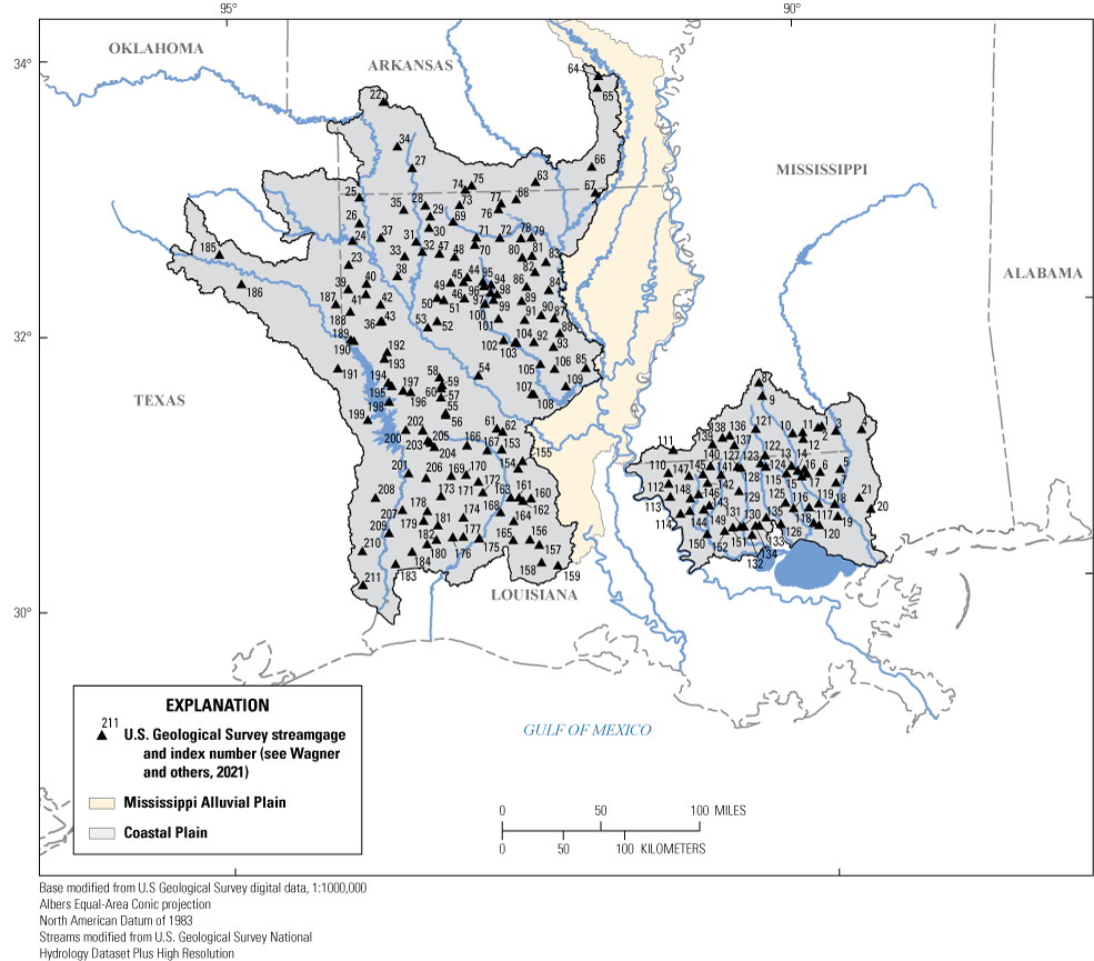
Figure 1. The Coastal Plain region includes most of Louisiana, and hundreds of streamgages
are in the region. — Figure 1.
Louisiana and surrounding States and locations of streamgages used in this study for the Coastal Plain region of Louisiana.

Louisiana has a humid subtropical climate, with an average annual temperature range from 64 degrees Fahrenheit (°F) in the north to 71 °F in the south near the mouth of the Mississippi River. The highest monthly average temperature is 82 °F in July, and the lowest monthly average temperature is 50 °F in January (https://www.britannica.com/place/Louisiana-state/Climate). The average annual rainfall in Louisiana ranges from 48 inches in the north to 75 inches in the south. Rainfall occurs throughout the year, with a predominantly wet season from April to September. Hurricane season runs from June 1 to November 30 (https://www.weather-us.com/en/louisiana-usa-climate#climate_text_1).

Previous Investigations

This is the sixth in a series of flood-frequency reports for Louisiana streams. The first two reports used the index-flood method to estimate flood quantiles at ungaged locations (Cragwall, 1952; Sauer, 1964). The third, fourth, and fifth reports, by Neely (1976), Lee (1985), and Ensminger (1998), respectively, used the LP3 distribution for flood-frequency analysis of annual peak-streamflow data from streamgages, per guidelines for flood-frequency analysis by Federal agencies outlined in Bulletin 17B (Interagency Advisory Committee on Water Data, 1982). In these latest three studies, ordinary least-squares (OLS) regression techniques were used to develop regression equations for estimating AEPs at ungaged locations on streams in Louisiana. Methods for estimating the magnitude and frequency of floods in small watersheds in Louisiana for drainage basins less than 10 square miles (mi²) were also previously developed by using OLS regression (Lowe, 1979).

Annual Peak-Streamflow Data

Streamgage Selection

A total of 211 USGS streamgages with 10 or more years of annual peak-streamflow data through the 2016 water year were used in this analysis: 176 in Louisiana, 18 in Mississippi, 9 in Arkansas, and 8 in Texas (fig. 1). Streamgages were either continuous-record or crest-stage gages and may have been operated as both during the period of record. Continuous-record streamgages are equipped with instrumentation that records the water-surface elevation, or stage, of the stream at fixed time intervals, typically every 15 minutes. The stage data are transmitted by satellite to the local USGS offices, at which time a streamflow is associated with each recorded stage value. Crest-stage gages only record the peak stages of floods. To determine the peak streamflow associated with a given peak-stage value, peak-stage to peak-streamflow relations, or “ratings,” are developed from direct or indirect measurements of peak streamflow made across the range of peak stages measured at the crest-stage gage.

Initially, streamflow data from 296 streamgages that had 10 or more years of annual peak-streamflow data (systematic and historical peaks) through the end of the 2016 water year were considered for analysis. Annual peak-streamflow data for the streamgages were downloaded from the USGS National Water Information System database (USGS, 2017a), and the drainage areas and locations of the basins associated with each streamgage were reviewed for redundancy.

Candidate streamgages were screened for redundancy, which occurs when the drainage basin of one streamgage is contained inside the drainage basin of another (nested) and the two basins are similar in size. When pairs of streamgages in basins are redundant, a statistical analysis assuming both streamgages are independent incorrectly represents the independent AEP streamflow information in the regional dataset (Gruber and Stedinger, 2008). To determine if two streamgages were redundant and thus represented the same hydrologic conditions, two types of information were considered: (1) the standardized distance between nested streamgages, and (2) the ratio of the basin drainage areas. The standardized distance between the centroids of the basins is defined as

S D_{i j} = \frac{D_{i j}}{\sqrt{0.5 (D R N A R E A_{i} + D R N A R E A_{j})}}

(1)

where

SD_{i j}: is the standardized distance between centroids of basin i and basin j (unitless),
D_{i j}: is the distance between centroids of basin i and basin j, in miles,
DRNAREA_i: is the geographic information system (GIS)-derived drainage area at site i, in square miles, and
DRNAREA_j: is the GIS-derived drainage area at site j, in square miles.

The drainage area ratio maximum (DARMAX) was used to determine if two nested basins are sufficiently similar in size to conclude they are essentially the same basin for the purposes of developing a regional hydrologic model (Veilleux, 2009). If the DARMAX is large enough, even if a pair of streamgages is nested, the streamgages will reflect different hydrologic responses because storms of different sizes and durations will affect each streamgage differently. The DARMAX is defined as

D A R M A X = M a x [\frac{D R N A R E A_{i}}{D R N A R E A_{j}}, \frac{D R N A R E A_{j}}{D R N A R E A_{i}}]

(2)

where

DARMAX: is the Max (maximum) of the two values in brackets,
DRNAREA_i: is the GIS-derived drainage area at site i, and
DRNAREA_j: is the GIS-derived drainage area at site j.

For this study, 33 pairs of streamgages having standardized distances less than or equal to 0.50 and DARMAX values less than or equal to 5 (Gruber and Stedinger, 2008) were considered redundant. One streamgage from each pair was removed based on the length and quality of streamflow record (Wagner and others, 2016). Following this review, 33 streamgages were removed for redundancy, and 52 others were removed because they were within the Mississippi Alluvial Plain flood region, for which a unique suite of GLS regression models was recently developed (Anderson, 2021). The final dataset for this study therefore consisted of 211 streamgages (fig. 1).

Trends in Annual Peak-Streamflow Data

When flood-frequency analyses are performed, annual peak-streamflow data are assumed to be stationary and their statistical properties unchanging over time (England and others, 2019). Therefore, trends in annual peak-streamflow data could bias the flood-frequency analyses; however, stationary, and nonstationary annual peak-streamflow data are often indistinguishable due to the paucity of observation records, except where changes in the underlying processes are so dramatic that no statistical assessment is necessary (Lins and Cohn, 2011). Streamflow records can exhibit multidecadal and century-scale variation, where multiyear periods in those records may show upward or downward trends that are not necessarily indicative of a persistent change in the system (Cohn and Lins, 2005). Annual peak-streamflow data can also exhibit serial correlation that can cause the Mann-Kendall test for monotonic trends to indicate a statistically significant trend when there is none (Hodgkins and Martin, 2003). For these reasons, results of the Mann-Kendall test were used to identify and screen stations with potentially significant (p-value < 0.05) anthropogenic effects on trends; upon further review, no streamgages were removed because of trends.

Regional Skew

Skew is a measure of the asymmetry of the probability distribution of a set of annual peak streamflows and is strongly affected by the presence of high or low outliers, among other factors; large positive station skew coefficients typically result from high outliers, and large negative station skew coefficients typically result from low outliers (Southard and Veilleux, 2014). Because it is sensitive to extreme flood events, the skew coefficient for limited annual peak-streamflow records may not provide an accurate estimate of the population, or “true,” skew; therefore, the Interagency Advisory Committee on Water Data recommends that the skew calculated from the annual peak-streamflow record at a streamgage (the station skew) be weighted with a regional skew determined by analysis of skew of annual peak-streamflow data from selected long-term streamgages in the study area, as detailed in Bulletin 17C (England and others, 2019). Weighted skew is determined by using the following equation:

G_{w} = \frac{M S E_{R} (G_{s}) + M S E_{S} (G_{R})}{M S E_{R} + M S E_{S}}

(3)

where

G_w: is the weighted skew,
G_s: is the station skew,
G_R: is the regional skew,
MSE_R: is the mean squared error of the regional skew, and
MSE_S: is the mean squared error of the station skew.

The regional skew map of the Nation published in Bulletin 17B was created by using streamgage data through the 1973 water year (Interagency Advisory Committee on Water Data, 1982, pl. 1). Since then, 47 additional years of annual peak-streamflow data have been collected, and the more rigorous B–WLS/B–GLS method has been developed that yields more accurate estimates of regional skew (Veilleux, 2009, 2011; Veilleux and others, 2011). The B–WLS/B–GLS method attempts to relate observed station skews to explanatory variables (basin characteristics). Since 2010, this GLS method has been successfully used to update regional skew in numerous States, including Arkansas and Louisiana (Wagner and others, 2016, appendix 1). In the Arkansas-Louisiana skew study, station skews from flood-frequency analysis of annual peak-streamflow records through the 2013 water year of 210 streamgages in Arkansas, Louisiana, southern Missouri, and eastern Oklahoma having minimal or no regulation or urbanization in their drainage basins were used. The regional skew is a constant value of −0.17 with a mean squared error of 0.348. The weighted skew coefficient is used within p-percent AEP analysis when estimating the LP3 frequency factor (K_p,Gw) for a given percentage (p) of the selected AEP.

Annual Exceedance Probability Analysis

Flood frequency for a stream having 10 or more years of peak-streamflow record is determined by fitting an LP3 frequency distribution to the base-10 logarithms (log) of annual peak-streamflow data as described in Bulletin 17C (England and others, 2019). This technique is generally accepted by most Federal and State agencies and has been in use by Federal agencies since 1982 (Interagency Advisory Committee on Water Data, 1982). The LP3 distribution is a three-moment distribution that requires estimating the population mean, standard deviation, and skew coefficient from the sample of logarithms of the annual peak streamflows from each streamgage (Parrett and others, 2011). The application of LP3, following Bulletin 17C guidelines, was facilitated by use of USGS PeakFQ software, version 7.3 (England and others, 2019).

In previous USGS reports regarding estimating flood magnitudes in Louisiana, the term “recurrence interval, in years” was used to characterize flood frequency; for example, a “100-year flood.” The USGS and other Federal agencies now refer to the p-percent AEP. For example, the 0.01 AEP has a 1-percent chance of occurring in any given year and corresponds to a recurrence interval of 100 years (reciprocal of 0.01; table 1) (Feaster and others, 2009). Over the duration of N years, the probability of a flood of a given magnitude occurring is expressed by the binomial distribution:

P

= [1− [1−(

AEP

)]

^N

]

(4)

where

AEP: is the annual exceedance probability for each year,
N: is the number of years, and
P: is a flood with probability of the AEP being equaled or exceeded over N years.

For example, by using equation 4, a flood having an AEP of 0.01 (1-percent; the 100-year flood), has a 26-percent {P= [1− [1−(.01)]³⁰]} probability of occurring within a 30-year period. The value of 26 percent is based on the binomial probability distribution that accounts for each of the 30 years having a 1-percent probability of the 100-year flood occurring (England and others, 2019).

Table 1.

Recurrence intervals with corresponding annual exceedance probability and p-percent chance exceedance for flood-frequency streamflow estimates (Feaster and others, 2009).

Table 1. Recurrence intervals with corresponding annual exceedance probability and p-percent chance exceedance for flood-frequency streamflow estimates (Feaster and others, 2009).
Recurrence interval, in years	Annual exceedance probability	p−Percent annual exceedance probability
2	0.5	50
5	0.2	20
10	0.1	10
25	0.04	4
50	0.02	2
100	0.01	1
200	0.005	0.5
500	0.002	0.2

Estimates of AEP streamflows corresponding to AEPs of 50-, 20-, 10-, 4-, 2-, 1, 0.5, and 0.2 percent (hereinafter, AEP streamflows are referred to as the “Q_{50-percent (%)},” “Q_20%,” “Q_10%,” “Q_4%,” “Q_2%,” “Q_1%,” “Q_0.5%,” and “Q_0.2%” streamflows, respectively) were computed for each streamgage by using the following equation:

log

Q_p=

\bar{X}

+K_p,Gw S

(5)

where

Q_p: is the p-percent AEP streamflow, in cubic feet per second;
$\bar{X}$: is the mean of the logarithms of the annual peak streamflow;
K_p,Gw: is an LP3 frequency factor based on the weighed skew coefficient (G_w) and the selected percentage (p) of the AEP, which can be obtained from appendix 3 of Bulletin 17B (Interagency Advisory Committee on Water Data, 1982); and
S: is the standard deviation of the logarithms of the annual peak streamflows.

Basin Characteristics

Nineteen basin characteristics were considered as potential explanatory variables and were selected based on hydrologic judgment of their anticipated relation to peak streamflow (table 2). The basin characteristics used in this study have maintained consistency with those available in StreamStats (USGS, 2017b). Arc Hydro Tools, version 2.0, was used to process the GIS layers to facilitate determination of basin characteristics. Arc Hydro Tools, version 2.0, is a set of utilities developed to operate in the ArcGIS, version 10.3.1, environment (Esri, 2009) and is described in detail by Eash and others (2013). The basin characteristics used in this study can be divided into three categories: morphometric (physical or shape), climatic/hydrologic, and soils and land use/land cover.

Table 2.

Basin and climatic characteristics tested as potential explanatory variables in generalized least-squares (GLS) regression analysis for the Coastal Plain region in Louisiana.

^{[NAD 83, North American Datum of 1983; NAVD 88, North American Vertical Datum of 1988]}

Table 2. Basin and climatic characteristics tested as potential explanatory variables in generalized least-squares (GLS) regression analysis for the Coastal Plain region in Louisiana.
Basin characteristic	Abbreviation	Units	Source of data
Area of drainage basin of a point on a stream	DRNAREA	square miles	Delineated by using Arc Hydro methods within Esri ArcGIS software (version 10.3.1 or later), 10-meter National Elevation Dataset (https://www.usgs.gov/core-science-systems/national-geospatial-program/national-map), and National Hydrography Dataset (https://www.usgs.gov/core-science-systems/ngp/national-hydrography)
Latitude of basin centroid	LAT_CENT	degrees relative to NAD 83	Determined from polygon representing drainage basin of streamgage by using Field Calculator in Esri ArcGIS software, version 10.3.1 or later
Longitude of basin centroid	LNG_CENT	degrees relative to NAD 83	Determined from polygon representing drainage basin of streamgage by using Field Calculator in Esri ArcGIS software, version 10.3.1 or later
Average land-surface elevation in drainage basin	ELEV	feet relative to the NAVD 88	Average elevation in drainage basin of stream point, computed in Esri ArcGIS by using 10-meter National Elevation Dataset, https://www.usgs.gov/core-science-systems/national-geospatial-program/national-map
Change in elevation divided by length between points 10 and 85 percent of distance along the longest flow path to the basin divide	CSL1085LFP	feet per mile	Computed by using Arc Hydro methods within Esri ArcGIS software (version 10.3.1 or later), 10-meter National Elevation Dataset (https://www.usgs.gov/core-science-systems/national-geospatial-program/national-map), and National Hydrography Dataset (https://www.usgs.gov/core-science-systems/ngp/national-hydrography)
Basin shape factor; square of the longest flow path from the stream point to the basin divide, divided by the area of the drainage basin	BSHAPELFP	unitless	Computed by using area of the drainage basin of the streamgage and length of the longest flow path in the basin as determined with Esri ArcGIS version 10.3.1
Soil hydrologic group	SOILINDEX	unitless	Basin-averaged soil hydrologic group computed from state soil geographic (STATSGO) gridded data, https://www.nrcs.usda.gov/wps/portal/nrcs/detail/soils/survey/geo/?cid=nrcs142p2_053629
Basin-averaged, mean annual precipitation for the period 1971−2000	PRECPRIS00	inches	30-Year normal precipitation from PRISM Climate Group, Oregon State University, https://prism.oregonstate.edu/normals/
Basin-averaged, 24-hour precipitation that is expected to occur, on average, once every 10 years	I24H10Y	inches	NOAA Atlas 14 precipitation frequency estimates, Precipitation Frequency Data Server, https://hdsc.nws.noaa.gov/hdsc/pfds/
Percentage of stream basin covered by impervious surface	LC11IMP	percent	2011 National Land Cover Database Urban Imperviousness, https://www.mrlc.gov/data?f%5B0%5D=category%3AUrban%20Imperviousness&f%5B1%5D=year%3A2011
Percentage of stream basin in forested land-use categories	LC11FOREST	percent	Sum of 2011 National Land Cover Database classes 41, 42, 43, https://www.mrlc.gov/data?f%5B0%5D=category%3ALand%20Cover&f%5B1%5D=year%3A2011
Percentage of stream basin covered in developed land use (open, low, medium, high development) in National Land Cover Database	LC11DEV	percent	Sum of 2011 National Land Cover Database classes 21−24, https://www.mrlc.gov/data?f%5B0%5D=category%3ALand%20Cover&f%5B1%5D=year%3A2011
Percentage of stream basin covered in open water, class 11, National Land Cover Database	LC11WATER	percent	Sum of 2011 National Land Cover Database classes 21−24, https://www.mrlc.gov/data?f%5B0%5D=category%3ALand%20Cover&f%5B1%5D=year%3A2011
Percentage of stream basin covered in barren land (rock/sand/clay)	LC11BARE	percent	2011 National Land Cover Database class 31, https://www.mrlc.gov/data?f%5B0%5D=category%3ALand%20Cover&f%5B1%5D=year%3A2011
Percentage of stream basin covered in areas dominated by shrubs	LC11SHRUB	percent	2011 National Land Cover Database class 52, https://www.mrlc.gov/data?f%5B0%5D=category%3ALand%20Cover&f%5B1%5D=year%3A2011
Percentage of stream basin covered in areas dominated by grasslands or herbacious vegetation	LC11GRASS	percent	2011 National Land Cover Database class 71, https://www.mrlc.gov/data?f%5B0%5D=category%3ALand%20Cover&f%5B1%5D=year%3A2011
Percentage of stream basin covered in areas of grasses, legumes, or grass-legume mixtures planted for livestock grazing or the production of seed or hay crops	LC11PAST	percent	2011 National Land Cover Database class 81, https://www.mrlc.gov/data?f%5B0%5D=category%3ALand%20Cover&f%5B1%5D=year%3A2011
Percentage of stream basin covered in areas used for the production of annual crops and perennial woody crops such as orchards or vineyards	LC11CROP	percent	Sum of 2011 National Land Cover Database classes 21−24, https://www.mrlc.gov/data?f%5B0%5D=category%3ALand%20Cover&f%5B1%5D=year%3A2011
Percentage of stream basin covered in wetlands	LC11WETLND	percent	Sum of 2011 National Land Cover Database classes 90 and 95, https://www.mrlc.gov/data?f%5B0%5D=category%3ALand%20Cover&f%5B1%5D=year%3A2011

Morphometric characteristics used to delineate accurate stream networks and basin boundaries were derived from two primary sources: (1) the 1:24,000-scale National Hydrography Dataset (USGS, 1999) and (2) the 10-meter National Elevation Dataset (USGS, 2009). From these sources, the drainage area (DRNAREA), length of the longest streamflow path in the drainage basin, change in elevation between points 10 and 85 percent along the longest streamflow path from the streamgage to the basin divide (CSL1085LFP), and mean elevations (ELEV) were computed for each stream basin. The basin shape factor (BSHAPELFP) computed as the ratio of the square of the length of the longest streamflow path to the drainage area of the basin, correlates to both the magnitude and arrival time of a peak streamflow (Southard and Veilleux, 2014).

Mean annual precipitation for the period 1971–2000 (PRECPRIS00) was averaged by basin using coverages from Parameter-Elevation Regressions on Independent Slopes Model (PRISM) data (PRISM Climate Group, 2013). The 10-year recurrence interval, 24-hour duration precipitation (I24H10Y) was averaged by basin using the annual maximum series of the National Oceanic and Atmospheric Administration (NOAA) Atlas 14 precipitation frequency estimates (NOAA, 2014). A mosaic of volumes 8 (Midwestern States) and 9 (Southeastern States) of Atlas 14 was created by using ArcGIS and was clipped to the study area boundary.

Soils and land use/land cover characteristics were obtained from three sources. The soil hydrologic group (SOILINDEX) was computed by using the Natural Resources Conservation Service State Soil Geographic (STATSGO) database (Schwarz and Alexander, 1995; U.S. Department of Agriculture, 2001). Percentages of urban (developed), forest, open water, and various vegetation land-use/land-cover types were computed for each basin in the study area by using the 2011 National Land Cover Database (Homer and others, 2015). For each basin, the sums of the percentages of low, medium, high, and open development (LC11DEV) and deciduous, evergreen, and mixed forest (LC11FOREST) were computed. Percentage of impervious surface (LC11IMP) was computed for each basin by using the National Land Cover Database 2011 Percent Developed Imperviousness layer (Xian and others, 2011).

Multicollinearity between explanatory parameters was evaluated by using the cor() function in the “smwrStats” package (Lorenz, 2013) for R (R Core Team, 2014). The cor() function compares all possible pairs of explanatory variables and computes Pearson’s correlation coefficient (also known as Pearson’s r). For pairs of explanatory variables with a correlation coefficient 0.50 < r < −0.50, only one explanatory variable was considered for use in the GLS regression analyses.

Ordinary Least-Squares Regression

OLS regression analysis was used to identify statistically significant explanatory variables (basin and climatic characteristics) and the best combinations of those variables to use in the final GLS equations. Criteria for OLS regression include (1) a linear relation between the explanatory (independent) variables and the response (dependent) variable (the p-percent AEP streamflow); (2) homoscedasticity (constant variance in the dependent variable across the range of the independent variables) about the regression line; and (3) normality of residuals (Southard and Veilleux, 2014). To meet these criteria, all variables were transformed to base-10 logarithms (log). The model used in the regression analysis is of the following form:

Q_p = aA^bB^c

(6)

where

Q_p: is the dependent variable, the p-percent AEP streamflow, in cubic feet per second;
A,B: are independent basin and climatic characteristics (explanatory variables); and
a,b,c: are regression coefficients.

If the dependent variable, Q_p, and the independent variables, A and B, are log transformed, the model takes the following form:

log

Q_p

= log(

a

) +

b

(log

A

) +

c

(log

B

)

(7)

where the explanatory variables are as previously defined.

The allReg() function in the “smwrStats” package (Lorenz, 2013) for R (R Core Team, 2014) was used to regress the Q_1% (the 100-year flood) against the suite of explanatory variables (basin and climatic characteristics) and determine the best 1-, 2-, 3-, 4-, and 5-variable combinations for estimating AEP streamflows. The Q_1% was selected for optimizing the selection of explanatory variables (p-value ≤ 0.05) because it is an important flood quantile used often by water managers, engineers, and planners (Eash and others, 2013). The best OLS 2- to 3- variable models determined with the “allReg()” function were subsequently used in the “lm()” function in the “stats” package for R to generate the full suite of performance metrics. OLS regression of the explanatory variables and the Q_1% indicated that a regression model using two explanatory variables, DRNAREA and CSL1085LFP, yielded the best performance metrics. Multicollinearity of explanatory variables was further evaluated by using the variance inflation factor (VIF; Helsel and others, 2020). For this study, it was desirable to keep the VIF at or below a value of approximately 5; OLS regression models indicated VIFs less than 5.09 for both DNRAREA and CSL1085LFP, which were deemed acceptable. For the 211 streamgages, the DRNAREA ranged from 0.01 to 1,899 mi², and the CSL1085LFP ranged from 1.20 to 273.6 feet per mile (Wagner and others, 2021).

Determination of Flood Regions

In developing regression equations for estimating AEP streamflows, dividing Louisiana into regions of relatively homogeneous flood hydrology can reduce model error (Eash and others, 2013). The previous flood-frequency investigation in Louisiana divided the State into two regions, “Pine Hills” and “Alluvial Plains” (Ensminger, 1998), the boundaries of which correspond roughly to those of the Coastal Plain and Mississippi Alluvial Plain regions described in this report (Fenneman and Johnson, 1946). In the 1998 study, OLS regression was used to test groupings of streamgages, using qualitative variables to represent the Pine Hills and Alluvial Plains regions. A similar qualitative analysis was conducted in this study and confirmed statistically significant hydrologic differences between streamgages located in the Coastal Plain and the Mississippi Alluvial Plain regions (fig. 1). Streamgages in the Mississippi Alluvial Plain were not considered in this study because flood-frequency regression equations for the Mississippi Alluvial Plain region were recently developed by Anderson (2021).

Generalized Least-Squares Regression Equations

Following the exploratory OLS regression of explanatory variables against the Q_1%, the at-site AEP streamflows for the 211 streamgages in this study were related to the explanatory variables DRNAREA and CSL1085LFP by using GLS multiple linear regression. Stedinger and Tasker (1985) showed that GLS regression provides more accurate estimates of regression coefficients and model standard error than OLS regression. OLS regression does not account for the sampling errors associated with estimates of AEP streamflows from streamgages with varying record lengths, nor does it account for the cross-correlation of concurrent annual peak streamflow between sites. GLS regression accounts for these errors by using a weighting matrix so that sites are weighted proportionally according to both the sampling errrors and cross-correlation of concurrent annual peak streamflows. The USGS weighted-multiple-linear regression program (WREG, version 1.05; https://water.usgs.gov/software/WREG/) was used to complete the GLS regression analysis (Eng and others, 2009; USGS, 2013). Unique GLS regression models were developed for each AEP streamflow (table 3). WREG uses a correlation smoothing function to relate the correlation between annual peak streamflows to the geographic distance between the centroids of the drainage basins of the streamgages. An alpha value of 0.003 and theta value of 0.983 were used in the WREG program for computing the correlation smoothing function. The final GLS regression models for estimating streamflow at ungaged locations yielded standard errors of prediction ranging from 39 to 53 percent for the Coastal Plain region of Louisiana. These results are like those from the previous study in Louisiana, which reported standard errors of prediction for the Pine Hills region (the equivalent of the Coastal Plain region in this study) of 41 to 57 percent (Ensminger, 1998). The relation between predicted and computed 1-percent AEP streamflow for the Coastal Plain region of Louisiana is shown in figure 2. The uncertainty of the regression is represented graphically as scatter of points along the 1:1 line.

Table 3.

Final generalized least-squares (GLS) regression models for estimating annual exceedance probability streamflows at ungaged locations on rural streams in the Coastal Plain region of Louisiana and associated performance metrics.

^{[AEPS, annual exceedance probability streamflow; MSE, mean squared error of unweighted
residuals; ft³/s, cubic feet per second; RMSE, root mean squared error of unweighted residuals;
AVP, average variance of prediction; SEP, average standard error of prediction; Pseudo-R², pseudo coefficient of determination; MEV, model error variance; SME, average standard
model error variance; Q_X%, annual exceedance probability streamflow of X percent; DRNAREA, area of drainage
basin of streamgage, in square miles; CSL1085LFP, change in elevation divided by length
between points 10 and 85 percent of the distance along the longest flow path to the
basin divide, in feet per mile]}

Table 3. Final generalized least-squares (GLS) regression models for estimating annual exceedance probability streamflows at ungaged locations on rural streams in the Coastal Plain region of Louisiana and associated performance metrics.
AEPS equations	MSE (log₁₀ ft³/s)	RMSE (percent)	Pseudo-R² (percent)	AVP (log₁₀ ft³/s)	SEP (percent)	MEV (log₁₀ ft³/s)	SME (percent)
Q_50% = (DRNAREA^0.701)(CSL1085LFP^0.252)10^2.001	0.0416	49.66	92.10	0.0342	44.60	0.0331	43.80
Q_20% = (DRNAREA^0.749)(CSL1085LFP^0.330)10^2.146	0.0341	44.53	94.06	0.0266	38.91	0.0256	38.10
Q_10% = (DRNAREA^0.774)(CSL1085LFP^0.372)10^2.216	0.0353	45.36	94.26	0.0263	38.66	0.0252	37.78
Q_4% = (DRNAREA^0.801)(CSL1085LFP^0.416)10^2.287	0.0398	48.49	93.70	0.0296	41.24	0.0283	40.26
Q_2% = (DRNAREA^0.817)(CSL1085LFP^0.442)10^2.332	0.0445	51.57	93.16	0.0329	43.63	0.0314	42.56
Q_1% = (DRNAREA^0.832)(CSL1085LFP^0.467)10^2.371	0.0498	55.00	92.60	0.0362	46.01	0.0346	44.87
Q_0.5% = (DRNAREA^0.845)(CSL1085LFP^0.488)10^2.405	0.0557	58.60	92.03	0.0397	48.40	0.0379	47.17
Q_0.2% = (DRNAREA^0.861)(CSL1085LFP^0.514)10^2.446	0.0640	63.57	90.93	0.0462	52.69	0.0442	51.36

Figure 2. Relation between predicted and computed 1-percent annual exceedance probability
streamflow for the Coastal Plain region; the uncertainty of the regression is represented
graphically as a scatter of points along the 1:1 line. — Figure 2.
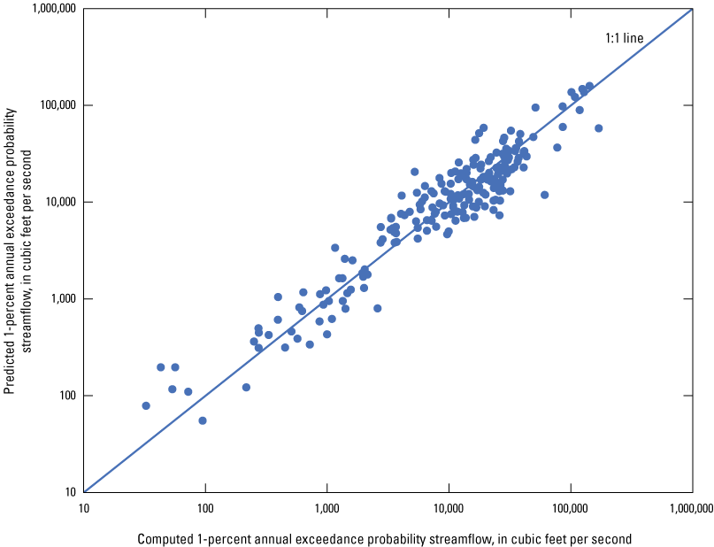
Relation between predicted and computed 1-percent annual exceedance probability streamflow for the Coastal Plain region in Louisiana.

The estimates of the Q_50%, Q_20%, Q_10%, Q_4%, Q_2%, Q_1%, Q_0.5% and Q_0.2% AEP streamflows for the 211 streamgages in this study are available in the associated data release (Wagner and others, 2021). These streamgages are in the Coastal Plain region of Louisiana and in the bordering States of Texas, Mississippi, and Arkansas. Basin and climatic characteristics, AEP streamflows, and PeakFQ input and output files for each station are also published in the associated data release (Wagner and others, 2021).

Application of Methods

When applying the GLS regression equations, users should be aware that the results may not be exact. Regression equations are statistical models that must be interpreted and applied within the limits of the data and with the understanding that the results are best-fit estimates with an associated variance. The regional regression equations are not valid where dams, flood-control structures, channelization, or diversion have a significant effect on annual peak streamflows or where drainage basins are considered urbanized. Computations of AEP at stations with a percent of impervious surfaces (LC11IMP) used the NLCD 2011 Percent Developed Imperviousness layer (Xian and others, 2011). Stations exceeding 10 percent impervious drainage area were considered urbanized and excluded from the study. Methods for estimating AEP streamflow differ for gaged locations on streams, ungaged locations on gaged streams, and locations on ungaged streams.

Gaged Locations

Accuracy of at-site AEP streamflow computed for a streamgage can be improved by weighting the at-site estimates of AEP streamflow with the GLS estimates. If the at-site and GLS estimates of a given AEP streamflow are weighted in an inverse proportion to the associated variances, the variance of the weighted estimate will be less than the variance of either the at-site or GLS estimates (Interagency Advisory Committee on Water Data, 1982). The weighted estimate is computed by using the following equation (England and others, 2019):

l o g Q_{p (g) w} = \frac{V P_{p (g) r} * l o g Q_{p (g) s} + V P_{p (g) s} * l o g Q_{p (g) r}}{V P_{p (g) r} + V P_{p (g) s}}

(8)

where

Q_p₍_g₎_w: is the weighted estimate for the selected p-percent AEP streamflow at streamgage (g), in cubic feet per second;
VP_p₍_g₎_r: is the variance of prediction for the p-percent AEP at streamgage (g) from the GLS regression model for the selected AEP, in log units.
Q_p₍_g₎_s: is the estimate for the selected p-percent AEP streamflow at streamgage (g) from the EMA analysis, in cubic feet per second;
VP _p₍_g)s: is the variance of prediction for the p-percent AEP at streamgage (g) from the EMA analysis, in log units; and
Q_p₍_g₎_r: is the estimate for the p-percent AEP streamflow at streamgage (g) from the GLS regression model, in cubic feet per second.

The variance of prediction of the weighted estimate for streamgage (g) (in log units) can be calculated as

V P_{p (g) w} = \frac{V P_{p (g) s} * V P_{p (g) r}}{V P_{p (g) s} + V P_{p (g) r}}

(9)

where

VP_p₍_g₎_w: is the variance of prediction for the weighted estimate of the p-percent AEP at streamgage (g), in log units.

A 95-percent confidence interval for the weighted estimate (in cubic feet per second) can be calculated as

95 %_{C I}_{u p p e r, i} = 10^{(l o g Q_{p (g) w} + 1.96 \sqrt{V P_{p (g) w}})}

(10)

95 %_{C I}_{l o w e r, i} = 10^{(l o g Q_{p (g) w} - 1.96 \sqrt{V P_{p (g) w}})}

where

$95 %_{C I}_{u p p e r, i}$: is the upper 95-percent confidence interval for the weighted estimate of the selected AEP streamflow at streamgage (g), in cubic feet per second; and
$95 %_{C I}_{l o w e r, i}$: is the lower 95-percent confidence interval for the weighted estimate of the selected AEP streamflow at streamgage (g), in cubic feet per second.

Ungaged Locations on Gaged Streams

The following method is recommended to improve AEP streamflow estimates for ungaged locations near a gaged station (Veilleux, 2009). To obtain a weighted AEP streamflow at the ungaged location (Q_p₍_u₎_w), the weighted AEP streamflow at the gaged site (Q_p₍_g₎_w) needs to be determined (Wagner and others, 2021). The following procedure is recommended if the drainage area at the ungaged location is within 50 percent of the drainage area at the gaged location. In other words, if the drainage area ratio $(\frac{D R N A R E A_{(u)}}{D R N A R E A_{(g)}})$ is more than 0.5 or less than 1.5, where DRNAREA₍_u₎ is the drainage area at the ungaged location, in square miles, and DRNAREA₍_g₎ is the drainage area at the streamgage location, in square miles, then the weighted flood estimate at the ungaged site can be computed by using the following equation:

Q_{p (u) w} = [(\frac{2 |Δ A|}{D R N A R E A_{(g)}}) + (1 - \frac{2 |Δ A|}{D R N A R E A_{(g)}}) (\frac{Q_{p (g) w}}{Q_{p (g) r}})] Q_{p (u) r}

(11)

where

Q_p₍_u₎_w: is the weighted AEP streamflow estimate at the ungaged location for the selected p-percent, in cubic feet per second;
Q_p₍_u₎_r: is the GLS streamflow estimate at the ungaged location for the selected p-percent, in cubic feet per second;
Q_p₍_g₎_w and Q_p₍_g₎_r: are as previously defined for equation 8; and
│ΔA│: is the absolute difference in drainage area between the ungaged location (DRNAREA₍_u₎) and the streamgage (DRNAREA₍_g₎) location, in square miles.

If the drainage area of an ungaged location differs by more than 50 percent from that of the streamgage location, the GLS equations in table 3 should be used. If an ungaged location is between two streamgages on the same stream, the site with the closest drainage area ratio and longest period of record should be used in equation 11 (Sauer, 1974).

Locations on Ungaged Streams

For locations on ungaged streams, the drainage area and slope should be determined using the same GIS datasets used in this study. The standard error of prediction is a measure of the accuracy of AEP streamflow estimates computed by using the regression equations (table 3). These equations apply to ungaged locations on gaged streams outside the range of 0.5 to 1.5 times the drainage area of the streamgage.

Accuracy and Limitations of Regional Regression Equations

Accuracy and limitations of the regression equations are affected by several factors. The equations are applicable at locations on streams in the Coastal Plain region of Louisiana where annual peak streamflows are not substantially affected by regulation, diversion, channelization, urbanization, backwater, storm surge, or tides. The accuracy of the GLS equations can only be assessed when the explanatory variables used are within the ranges of those used in their development (table 2; Wagner and others, 2021). AEP streamflow estimates for ungaged locations on streams in Louisiana will be available in StreamStats (https://water.usgs.gov/osw/streamstats/). StreamStats will use the same GIS datasets used in this study to calculate DRNAREA and CSL1085LFP to compute AEP streamflows at ungaged locations. Prior to the implementation of StreamStats, basin characteristics for ungaged locations should be measured using the same GIS datasets used in this study (table 2).

A measure of the uncertainty in the GLS equations is the prediction interval of the AEP streamflow and is the minimum and maximum value between a stated probability for which the true value of the AEP flow exists (Helsel and others, 2020). The prediction interval determines the range of streamflow values for a selected estimate given a confidence level and the standard error of prediction. For a 90-percent prediction interval, the true AEP streamflow has a 90-percent probability of being within the interval. The following equation can be used to compute the 90-percent prediction interval for an AEP streamflow estimate (modified from Tasker and Driver, 1988):

\frac{Q}{T}

<

Q

<

QT

(12)

where

Q: is the GLS estimate of the selected AEP streamflow at the ungaged location, in cubic feet per second, and the following equation can be used to compute T:

T = 10^{[t_{(α / 2, n - p)} S E P_{i}]}

(13)

where

t₍_α/2,n−p₎: is the critical value, t, from the student’s t-distribution at alpha level α (α=0.10 for the 90-percent prediction interval, critical values may be obtained in many statistical textbooks, or from the world wide web);
n−p: is the degree of freedom with n streamgages (211) included in the regression analysis and p explanatory parameters in the equation (the number of explanatory variables [2] plus one for the intercept, 3); and
SEP_i: is the standard error of prediction for site i (table 3).

The following equation can be used to compute SEP_i:

SEP_i

= [

MEV

+

X_iU X_i'

]

^0.5

(14)

where

MEV: is the model error variance from the GLS regression model for the selected AEP (table 4);
X_i: is the row vector for the streamgage i, starting with the number 1, followed by the log values of the two (2) explanatory variables used in the regression;
U: is the covariance matrix for the regression coefficients (table 4); and
X_i': is the matrix algebra transpose of X_i.

SEP_i represents the standard error of prediction, which is the sum of the model error and the sampling error for site i. The X_iUX_i' term in equation 14 is also referred to as the sampling error for site i. The value of t₍_α/2,n−p₎ is the critical value of the student’s t-distribution for α=0.10, n is the number of streamgages (n=211), and p number of explanatory parameters including the intercept (p=3). From the standard statistical t-tables, t₍_α/2,n−p₎ is 1.652. The values of U needed to determine the 90-percent prediction intervals for AEP streamflows estimated by using the GLS regression equations are provided (table 4).

Table 4.

Values used to determine prediction intervals of the regression equations presented in table 3.

^{[The covariance matrix, U, is used in equation 14; AEP is the annual exceedance probability; MEV is the regression equation model error
variance (table 3) used in equation 14]}

Table 4. Values used to determine prediction intervals of the regression equations presented in table 3.
AEP streamflow	MEV	U
Q_50%	0.0331	0.0101	−0.0028	−0.0062
		−0.0028	0.0009	0.0017
		−0.0062	0.0017	0.0043
Q_20%	0.0256	0.0084	−0.0023	−0.0052
		−0.0023	0.0007	0.0015
		−0.0052	0.0015	0.0036
Q_10%	0.0252	0.0088	−0.0024	−0.0054
		−0.0024	0.0008	0.0015
		−0.0054	0.0015	0.0038
Q_4%	0.0283	0.0104	−0.0029	−0.0063
		−0.0029	0.0009	0.0018
		−0.0063	0.0018	0.0044
Q_2%	0.0314	0.0118	−0.0032	−0.0072
		−0.0032	0.0010	0.0020
		−0.0072	0.0020	0.0050
Q_1%	0.0346	0.0132	−0.0036	−0.0081
		−0.0036	0.0012	0.0023
		−0.0081	0.0023	0.0056
Q_0.5%	0.0379	0.0147	−0.0040	−0.0090
		−0.0040	0.0013	0.0025
		−0.0090	0.0025	0.0063
Q_0.2%	0.0442	0.0171	−0.0047	−0.0105
		−0.0047	0.0015	0.0030
		−0.0105	0.0030	0.0073

Summary

Methods for estimating the magnitude and frequency of floods at ungaged locations on rural streams in Louisiana were last updated in 1998. Since then, many years of additional annual peak-streamflow data have been collected at streamgages, and new statistical methods have been developed for flood-frequency analysis. Additionally, new and updated climatic and land-use/land-cover data have become available for use as explanatory variables (basin characteristics). Thus, the U.S. Geological Survey (USGS), in cooperation with the Louisiana Department of Transportation and Development, began a study to update regression equations that can be used to estimate streamflows corresponding to selected annual exceedance probabilities (AEPs) at ungaged locations on streams in the Coastal Plain region of Louisiana. The USGS software PeakFQ, version 7.3, was used to conduct flood-frequency analysis of annual peak-streamflow records from 211 streamgages operated by the USGS in Louisiana and surrounding States that were not substantially affected by regulation, diversion, channelization, backwater, tides, or urbanization. The expected moments algorithm (EMA), multiple Grubbs-Beck test for potentially influential low floods, and the most recent regional skew applicable to the study area were used in the flood-frequency analysis in PeakFQ. EMA estimates of streamflows corresponding to the 50-, 20-, 10-, 4-, 2-, 1-, 0.5-, and 0.2-percent AEPs (AEP streamflows of the 2-, 5-, 10-, 25-, 50-, 100-, 200-, and 500-year floods, respectively) were then used to develop regression models for estimating AEP streamflows at ungaged locations.

Ordinary least-squares regression and categorical variables were used to confirm the statistical significance of two flood regions in the study area, the Coastal Plain and Mississippi Alluvial Plain regions, which was consistent with the previous study completed in 1998. Regression models were developed using 211 streamgages in the Coastal Plain region of Louisiana and neighboring States; regression models for the Mississippi Alluvial Plain region were developed in 2021. The allReg() function in the USGS “smwrStats” package for R used ordinary least-squares regression to test 19 potential explanatory variables (basin characteristics) for statistical significance and determine the best 1-, 2-, 3-, 4-, and 5-variable combinations for estimating AEP streamflows. A 2-variable model incorporating drainage area and channel slope as explanatory variables yielded superior performance metrics. Drainage area of the 211 streamgages used in the study ranged from 0.011 to 1,899 square miles, and channel slopes ranged from 1.16 to 273.6 feet per mile.

The generalized least-squares (GLS) regression models were generated by using the USGS weighted-multiple-linear regression (WREG) software in the R environment. Standard errors of prediction ranged from 39 to 53 percent and are similar to the standard errors of prediction for the Pine Hills region from the 1998 study (the equivalent of the Coastal Plain region in this study) of 41 to 57 percent.

The GLS regression models presented in this study apply to locations on streams in Louisiana where annual peak streamflows are not substantially affected by regulation, diversion, channelization, backwater, tides, storm surge, or urbanization. The applicability and accuracy of the GLS regression models depend on the basin characteristics measured for an ungaged location on a stream being within the range of those used to develop the equations. Methods are presented for using the GLS regression equations to weight at-site estimates of AEP streamflows at streamgage locations and compute AEP streamflows for ungaged locations on gaged and ungaged streams.

References Cited

Anderson, B.T., 2021, Magnitude and frequency of floods in the alluvial plain of the lower Mississippi River, 2017: U.S. Geological Survey Scientific Investigations Report 2021–5046, 15 p., accessed May 2024 at https://doi.org/10.3133/sir20215046.

Cohn, T.A., England, J.F., Berenbrock, C.E., Mason, R.R., Stedinger, J.R., and Lamontagne, J.R., 2013, A generalized Grubbs-Beck test statistic for detecting multiple potentially influential low outliers in flood series: Water Resources Research, v. 49, no. 8, p. 5047–5058, accessed October 22, 2015, at https://onlinelibrary.wiley.com/doi/10.1002/wrcr.20392/abstract.

Cohn, T.A., Lane, W.L., and Baier, W.G., 1997, An algorithm for computing moments-based flood quantile estimates when historical flood information is available: Water Resources Research, v. 33, no. 9, p. 2089–2096.

Cohn, T.A., and Lins, H.F., 2005, Nature’s style—Naturally trendy: Geophysical Research Letters, v. 32, article L23402, p. 1–5, accessed June 6, 2018, at https://agupubs.onlinelibrary.wiley.com/doi/epdf/10.1029/2005GL024476.

Cragwall, J.S., 1952, Floods in Louisiana, magnitude and frequency: Louisiana Department of Highways, 281 p.

Eash, D.A., Barnes, K.K., and Veilleux, A.G., 2013, Methods for estimating annual exceedance-probability streamflows for streams in Iowa, based on data through water year 2010: U.S. Geological Survey Scientific Investigations Report 2013–5086, 63 p., 1 app.

Eng, K., Chen, Y.-Y., and Kiang, J.E., 2009, User’s guide to the weighted-multiple-linear regression program (WREG version 1.0): U.S. Geological Survey Techniques and Methods, book 4, chap. A8, 21 p., accessed October 26, 2018, at https://pubs.usgs.gov/tm/tm4a8/.

England, J.F., Jr., Cohn, T.A., Faber, B.A., Stedinger, J.R., Thomas, W.O., Jr., Veilleux, A.G., Kiang, J.E., and Mason, R.R., Jr., 2019, Guidelines for determining flood flow frequency—Bulletin 17C (ver. 1.1, May 2019): U.S. Geological Survey Techniques and Methods, book 4, chap. B5, 148 p., accessed April 9, 2019, at https://pubs.usgs.gov/tm/04/b05/tm4b5.pdf.

Ensminger, P.A., 1998, Floods in Louisiana, magnitude and frequency (5th ed.): Louisiana Department of Transportation and Development Water Resources Technical Report no. 60, 333 p.

Esri, 2009, ArcGIS desktop help: Esri web page, accessed November 23, 2015, at https://desktop.arcgis.com/en/arcmap/.

Feaster, T.D., Gotvald, A.J., and Weaver, J.C., 2009, Magnitude and frequency of rural floods in the Southeastern United States, 2006—Volume 3, South Carolina: U.S. Geological Survey Scientific Investigations Report 2009–5156, 226 p., accessed June 16, 2021, at https://pubs.usgs.gov/sir/2009/5156/pdf/sir2009-5156.pdf.

Fenneman, N.M., and Johnson, D.W., 1946, Physical division of the United States: U.S. Geological Survey map, scale 1:7,000,000.

Gruber, A.M., and Stedinger, J.R., 2008, Models of LP3 regionalized skew, data selection and Bayesian GLS regression, in Babcock, R.W., and Watson, R., eds., World Environmental and Water Resources Congress, Honolulu, Hawai’i, May 12–16, 2008: Paper 596, 10 p.

Helsel, D.R., Hirsch, R.M., Ryberg, K.R., and Archfield, S.A., 2020, Statistical methods in water resources: U.S. Geological Survey Techniques of Water-Resources Investigations, book 4, chap. A3, 458 p., accessed April 13, 2021, at https://pubs.usgs.gov/tm/04/a03/tm4a3.pdf.

Hodgkins, G.A., and Martin, G.R., 2003, Estimating the magnitude of peak flows for streams in Kentucky for selected recurrence intervals: U.S. Geological Survey Water-Resources Investigations Report 2003–4180, 73 p.

Homer, C.G., Dewitz, J.A., Yang, L., Jin, S., Danielson, P., Xian, G., Coulston, J., Herold, N.D., Wickham, J.D., and Megown, K., 2015, Completion of the 2011 National Land Cover Database for the conterminous United States—Representing a decade of land cover change information: Photogrammetric Engineering and Remote Sensing, v. 81, no. 5, p. 345–354, accessed July 21, 2020, at https://www.researchgate.net/profile/Limin_Yang5/publication/282254893_Completion_of_the_2011_National_Land_Cover_Database_for_the_Conterminous_United _States_-_Representing_a_Decade_of_Land_Cover_Change_Information/links/5693bbc808aeab58a9a2a661/Completion-of-the-2011-National-Land-Cover-Database-fo r-the-Conterminous-United-States-Representing-a-Decade-of-Land-Cover-Change-Information.pdf.

Interagency Advisory Committee on Water Data, 1982, Guidelines for determining flood flow frequency—Bulletin 17B of the Hydrology Subcommittee: U.S. Geological Survey, Office of Water Data Coordination, 183 p., accessed April 9, 2019, at https://water.usgs.gov/osw/bulletin17b/dl_flow.pdf.

Lee, F.N., 1985, Floods in Louisiana, magnitude and frequency (4th ed.): Louisiana Department of Transportation and Development Water Resources Technical Report no. 36, 30 p.

Lins, H.F., and Cohn, T.A., 2011, Stationarity—Wanted dead or alive?: Journal of the American Water Resources Association (JAWRA), v. 47, no. 3, p. 475–480, accessed October 26, 2018, at https://onlinelibrary.wiley.com/doi/abs/10.1111/j.1752-1688.2011.00542.x.

Lorenz, D.L., 2013, smwrStats—An R package for the analysis of hydrologic data, version 0.6: U.S. Geological Survey software release, accessed October 26, 2015, at https://github.com/USGS-R/smwsStats.

Lowe, A.S., 1979, Magnitude and frequency of floods for small watersheds in Louisiana: Louisiana Department of Transportation and Development, Office of Highways Research Study no. 65–2H, 52 p.

National Oceanic and Atmospheric Administration [NOAA], 2014, Precipitation Frequency Data Server—NOAA Atlas 14 precipitation frequency estimates in GIS compatible format: National Oceanic and Atmospheric Administration, National Weather Service Hydrometeorological Design Studies Center online database, accessed December 2, 2014, at http://hdsc.nws.noaa.gov/hdsc/pfds/pfds_gis.html.

Neely, B.L., Jr., 1976, Floods in Louisiana, magnitude and frequency (3d ed.): Louisiana Department of Highways, 340 p.

Parrett, C., Veilleux, A., Stedinger, J.R., Barth, N.A., Knifong, D.L., and Ferris, J.C., 2011, Regionalized skew for California, and flood-frequency for selected sites in the Sacramento–San Joaquin River Basin, based on data through water year 2006: U.S. Geological Survey Scientific Investigations Report 2010–5260, 94 p.

PRISM Climate Group, 2013, PRISM climate data: Corvallis, Oregon, Oregon State University, accessed January 26, 2013, at http://prism.oregonstate.edu.

R Core Team, 2014, The R project for statistical computing: Vienna, Austria, The R Foundation for Statistical Computing web page, accessed April 8, 2021, at http://www.R-project.org/.

Sauer, V.B., 1964, Floods in Louisiana—Magnitude and frequency (2d ed.): Louisiana Department of Highways, 402 p.

Sauer, V.B., 1974, Flood characteristics of Oklahoma streams, techniques for calculating magnitude and frequency of floods in Oklahoma, with compilations of flood data through 1971: U.S. Geological Survey Water-Resources Investigations Report 73–52, 307 p.

Schwarz, G.E., and Alexander, R.B., 1995, State soil geographic (STATSGO) data base for the conterminous United States: U.S. Geological Survey Open-File Report 95–449, 95 p.

Southard, R.E., and Veilleux, A.G., 2014, Methods for estimating annual exceedance-probability flows and largest recorded floods for unregulated streams in rural Missouri: U.S. Geological Survey Scientific Investigations Report 2014–5165, 39 p., accessed October 25, 2021, at https://doi.org/10.3133/sir20145165.

Stedinger, J.R., and Tasker, G.D., 1985, Regional hydrologic analysis—1. Ordinary, weighted, and generalized least squares compared: Water Resources Research, v. 21, no. 9, p. 1421–1432, accessed October 26, 2015, at https://doi.org/10.1029/WR021i009p01421.

Tasker, G.D., and Driver, N.E., 1988, Nationwide regression models for predicting urban runoff water quality at unmonitored sites: Journal of the American Water Resources Association, v. 24, no. 5, p. 1091–1101.

U.S. Department of Agriculture, 2001, State Soil Geographic (STATSGO) data base—Data use information: Natural Resources Conservation Service, National Soil Survey Center, Miscellaneous Publication no. 1492, 110 p.

U.S. Geological Survey [USGS], 1999, The National Hydrography Dataset: U.S. Geological Survey Fact Sheet 106–99, 2 p., accessed November 12, 2020, at http://pubs.er.usgs.gov/publication/fs10699.

U.S. Geological Survey [USGS], 2009, The National Map Download, v. 2.0: U.S. Geological Survey online database, accessed October 21, 2015, at https://viewer.nationalmap.gov/basic/.

U.S. Geological Survey [USGS], 2013, WREG, weighted-multiple-linear regression program: U.S. Geological Survey software release, accessed June 1, 2014, at https://water.usgs.gov/software/WREG/.

U.S. Geological Survey [USGS], 2017a, USGS water data for the Nation: U.S. Geological Survey National Water Information System database, accessed November 8, 2017, at https://doi.org/10.5066/F7P55KJN.

U.S. Geological Survey [USGS], 2017b, Welcome to StreamStats: U.S. Geological Survey online database, accessed November 11, 2020, at https://water.usgs.gov/osw/streamstats/.

Veilleux, A.G., 2009, Bayesian GLS regression for regionalization of hydrologic statistics, floods, and Bulletin 17B skew: Ithaca, New York, Cornell University, master’s thesis, 155 p.

Veilleux, A.G., 2011, Bayesian GLS regression, leverage, and influence for regionalization of hydrologic statistics: Ithaca, New York, Cornell University, Ph.D. dissertation, 184 p.

Veilleux, A.G., Stedinger, J.R., and Lamontagne, J.R., 2011, Bayesian WLS/GLS regression for regional skewness analysis for regions with large cross-correlations among flood flows, in World Environmental and Water Resources Congress, Palm Springs, California, May 22–26, 2011: Paper 3103, p. 3103–3112.

Wagner, D.M., Ensminger, P.A., and Whaling, A.R., 2021, Flood-frequency of rural, non-tidal streams in Louisiana and part of Arkansas, Mississippi, and Texas, 1877–2016: U.S. Geological Survey data release, https://doi.org/10.5066/P9B48P2W.

Wagner, D.M., Krieger, J.D., and Veilleau, A.G., 2016, Methods for estimating annual exceedance probability discharges for streams in Arkansas, based on data though water year 2013: U.S. Geological Survey Scientific Investigations Report 2016–5081, 136 p. [Also available at https://pubs.usgs.gov/sir/2016/5081/sir20165081.pdf.]

Xian, G., Homer, C., Dewitz, J., Fry, J., Hossain, N., and Wickham, J., 2011, The change of impervious surface area between 2001 and 2006 in the conterminous United States: Photogrammetric Engineering and Remote Sensing, v. 77, no. 8, p. 758–762.

Conversion Factors

Inch/Pound to International System of Units


Multiply	By	To obtain
Length
inch (in.)	2.54	centimeter (cm)
foot (ft)	0.3048	meter (m)
mile (mi)	1.609	kilometer (km)
Area
square mile (mi²)	259.0	hectare (ha)
square mile (mi²)	2.590	square kilometer (km²)
Flow rate
cubic foot per second (ft³/s)	0.02832	cubic meter per second (m³/s)
Hydraulic gradient
foot per mile (ft/mi)	0.1894	meter per kilometer (m/km)

Temperature in degrees Fahrenheit (°F) may be converted to degrees Celsius (°C) as follows:

°C = (°F – 32) / 1.8.

Datum

Vertical coordinate information is referenced to the North American Vertical Datum of 1988 (NAVD 88).

Horizontal coordinate information is referenced to the North American Datum of 1983 (NAD 83).

Elevation, as used in this report, refers to the distance above a vertical datum.

Supplemental Information

Water year: A 1-year period from October 1 to September 30, defined by the year in which it ends; for example, the 2016 water year is the period October 1, 2015–September 30, 2016.

Abbreviations

<: less than
≤: less than or equal to
%: percent
AEP: annual exceedance probability
B–WLS/B–GLS: Bayesian weighted least squares/Bayesian generalized least squares
CSL1085LFP: Change in elevation between points 10 and 85 percent of the distance along the main channel from the streamgage to the basin divide, divided by the length between the points, in miles
DARMAX: drainage area ratio maximum
DRNAREA: drainage area
EMA: expected moments algorithm
GIS: geographic information system
GLS: generalized least squares
log: base-10 logarithms
LP3: log-Pearson III
MEV: model error variance
OLS: ordinary least squares
p: given percentage
r: Pearson’s correlation coefficient
USGS: U.S. Geological Survey
VIF: variance inflation factor
WREG: weighted-multiple-linear regression program

For more information about this publication, contact

Director, Lower Mississippi-Gulf Water Science Center

U.S. Geological Survey

640 Grassmere Park, Suite 100

Nashville, TN 37211

For additional information, visit

https://www.usgs.gov/centers/lmg-water/

Publishing support provided by

Lafayette Publishing Service Center

Disclaimers

Any use of trade, firm, or product names is for descriptive purposes only and does not imply endorsement by the U.S. Government.

Although this information product, for the most part, is in the public domain, it also may contain copyrighted materials as noted in the text. Permission to reproduce copyrighted items must be secured from the copyright owner.

Suggested Citation

Ensminger, P.A., Wagner, D.M., and Whaling, A., 2024, Magnitude and frequency of floods in the Coastal Plain region of Louisiana, 2016: U.S. Geological Survey Scientific Investigations Report 2024–5031, 18 p., https://doi.org/10.3133/sir20245031.

ISSN: 2328-0328 (online)

Study Area

Additional publication details
Publication type	Report
Publication Subtype	USGS Numbered Series
Title	Magnitude and frequency of floods in the Coastal Plain region of Louisiana, 2016
Series title	Scientific Investigations Report
Series number	2024-5031
DOI	10.3133/sir20245031
Year Published	2024
Language	English
Publisher	U.S. Geological Survey
Publisher location	Reston, VA
Contributing office(s)	Lower Mississippi-Gulf Water Science Center
Description	Report: viii, 18 p.; 2 Data Releases
Country	United States
State	Arkansas, Louisiana, Mississippi, Texas
Online Only (Y/N)	Y
Google Analytic Metrics	Metrics page

Magnitude and Frequency of Floods in the Coastal Plain Region of Louisiana, 2016

Table of Contents

Links

Acknowledgments

Abstract

Introduction

Purpose and Scope

Description of Study Area

Previous Investigations

Annual Peak-Streamflow Data

Streamgage Selection

(1)

(2)

Trends in Annual Peak-Streamflow Data

Regional Skew

(3)

Annual Exceedance Probability Analysis

(4)

Table 1.

(5)

Basin Characteristics

Table 2.

Ordinary Least-Squares Regression

(6)

(7)

Determination of Flood Regions

Generalized Least-Squares Regression Equations

Table 3.

Application of Methods

Gaged Locations

(8)

(9)

(10)

Ungaged Locations on Gaged Streams

(11)

Locations on Ungaged Streams

Accuracy and Limitations of Regional Regression Equations

(12)

(13)

(14)

Table 4.

Summary

References Cited

Conversion Factors

Datum

Supplemental Information

Abbreviations

Disclaimers

Suggested Citation

Study Area