

A Model Uncertainty Quantification Protocol for Evaluating the Value of Observation Data
Links
- Document: Report (7.93 MB pdf) , HTML , XML
- NGMDB Index Page: National Geologic Map Database Index Page (html)
- Download citation as: RIS | Dublin Core
Acknowledgments
The authors appreciate support and funding from the Mississippi Alluvial Plain project and the HyTEST Project as part of the Integrated Water Prediction Water Resources Mission Area program. Wade Kress and J.R. Rigby of the U.S. Geological Survey provided valuable management support. Technical reviews by Kalle Jahn and Moussa Guira of the U.S. Geological Survey were helpful.
Abstract
The history-matching approach to parameter estimation with models enables a powerful offshoot analysis of data worth—using the uncertainty of a model forecast as a metric for the worth of data. Adding observation data will either have no impact on forecast uncertainty or will reduce it. Removing existing data will either have no impact on forecast uncertainty or will increase it. The history-matching framework makes it possible to perform this quantitative analysis leveraging the connections among observations, model parameters, and model forecasts. We show this behavior on a specific groundwater flow model of the Mississippi Alluvial Plain and show where the analysis can be informative for considering the potential design of an observation network based on existing or potential observations.
Introduction
The Mississippi Alluvial Plain (MAP) project is a large, multi-disciplinary project with the goal of supporting stakeholder-driven decision support for water-resource management. This project includes endpoints of streamflow depletion and drawdown as forecasts that can be managed through land-use and water-management changes, guided by economic tradeoffs. In this report, we examine the theory and practice of using mathematical techniques with a groundwater-flow model to evaluate the relative worth of existing and potential observation data that can be used for parameter estimation through history matching. The metric of reducing forecast uncertainty is used to evaluate data worth.
Purpose and Scope
This document is intended to provide the theoretical background for evaluating forecast uncertainty with models. In particular, this project is motivated by a desire for models to be dynamic and “living” such that over the course of a project, the models not only serve the needs of making forecasts, but the quality of those forecasts can guide data collection throughout the project.
The examples in this work are based on a regional groundwater-surface water project with a groundwater-flow model (Hunt and others, 2021) and a soil-water balance model (Nielsen and Westenbroek, 2023). However, the techniques presented here can be used with a range of models and the tools are generally model-independent.
A Note on Software Packages Used
The workflows in this document use the open-source scripting environment of the Python and the PEST/PEST++ suite of programs (Doherty, 2010a; Doherty and others, 2011; Welter and others, 2012; White and others, 2020; https://github.com/usgs/pestpp) which interface with the utility software PyEMU (White and others, 2016; https://github.com/pypest/pyemu). These tools were chosen because they are model-independent, free, and open-source. Model independence has been a feature of the PEST suite of tools from its inception, and the techniques documented here can be applied to any models.
Background Mathematics
The mathematics behind linear and nonlinear uncertainty methods are rooted in considering quantities related to models (for example, input parameters, model outputs collocated with observations, and outputs making forecasts) as random variables. This means we not only consider the base values of these quantities, but also their uncertainty (expressed as variance or covariance).
Distributions
In this work, Gaussian (Normal) and Uniform Probability Density Functions (Distributions) are used to describe random variables.
For a single (scalar) value, the Gaussian distribution is
whereis a Normal Distribution of conditional on and ,
θ
is the random variable,
µ
is the mean, and
σ2
is the variance.
For a vector of multiple values, the multivariate Gaussian distribution is
whereis a Normal Distribution of θ conditional on µ and Σ,
𝛉
is the vector of k random variables,
µ
is the vector of k mean values,
𝚺
is the k×k covariance matrix, and
T
is a matrix transpose.
For a single (scalar) value, the Uniform Distribution is
whereLocal Sensitivity and the Jacobian Matrix
PEST is based on the Gauss-Levenberg-Marquardt technique for damped least-squares regression. Fienen and others (2024) provide a derivation and interpretation of the algorithm. This is a gradient-based algorithm that depends on parameter sensitivity to supply the gradients. The parameter sensitivity of the modeled output m(θ) (collocated in space and time with observation z) to model input parameter θ is defined as
This sensitivity is commonly approximated using finite differences by perturbing a parameter by a small increment Δθ as
whereThe Jacobian matrix (J) is constructed of the local sensitivity of all pairs of observations with parameters forming a matrix:
wherei
ranges from 1 to the number of observations (NOBS), and
j
ranges from 1 to the number of adjustable parameters (NPAR).
At its root, the Jacobian matrix can be interpreted as the basis for an approximation for a mapping from used in the change of variables for integration in calculus (the determinant of the Jacobian matrix provides the actual mapping if the Jacobian is a square matrix; Simmons, 1985, p. 673). In the context of parameter estimation, this matrix not only provides the gradients needed to find a solution to the inverse problem, but also serves as an approximate mapping from observation space to parameter space (for example, ), thus projecting information from a set of observation data to a set of parameter data. If the system were totally linear, then this mapping would be complete and a unique mapping would result in a calibrated model in one step. However, this is not the case, as discussed briefly below in the Parameter Estimation—Gauss-Levenberg-Marquardt Algorithm section (and in more detail in Fienen and others, 2024), so the mapping of observation information to parameters is approximate. That approximation, when adjusted based on assumed uncertainty of observation data, is a powerful one and can inform the likely quality of a parameter-estimation effort. This approximation can map the uncertainty of observation data onto parameter data and, similarly, project that out to model forecasts.
Forecast Sensitivity
A similar calculation can also be made to determine the sensitivity of a model forecast (s) to the model and parameters (θ) also using the finite-difference approximation
where, in this case,Similar to local sensitivity of model observations, this calculation is made entirely from adjusting parameters and calculating model outputs. As a result, there is no need for an independent estimate of the forecast value to calculate this sensitivity.
Parameter Estimation—The Objective Function
The parameter-estimation process entails the finding of the set of parameter values that minimizes an objective function. The objective function (Φ) is a metric of weighted, squared differences between observations (z) and modeled equivalents to them :
whereΣϵ
is the covariance matrix of observation errors (ϵ), which are, in practice, typically assumed independent and normally distributed.
The diagonal variance values σ2 constituting Σϵ are informed to the PEST and PyEmu programs as weights, defined as , where σ is an estimate of the standard deviation of the observed value. The matrix Σϵ has σ2 for each observation on the diagonal. This value of σ corresponds with the epistemic error that encapsulates measurement error and assumed errors in the model (for example, Doherty and Welter, 2010; White and others, 2014). As a result, the covariance matrices are metrics of error or uncertainty.
Parameter Estimation—Gauss-Levenberg-Marquardt Algorithm
To find the parameters that minimize Φ (eq. 8) for a linear case, the best estimate of parameters is available using the Gauss-Newton method as
For nonlinear cases, a Taylor expansion is repeatedly iterated about an initial estimate of parameters (x0). For an incremental step to new parameters
whereRearranging this to iteratively solve for parameters θ, each subsequent iteration takes the form of
whereis recalculated at each iteration using the most recent estimate of parameters available , and
λ
is the Marquardt adjustment that adjusts the solution trajectory between the Newton direction and the steepest descent direction.
This iterative procedure accounts for the nonlinearity of the problem. For a linear problem, would not change with changing parameter values. The inverse problem is solved making use of just these few pieces of information: , Σϵ, and z. As a result, much information regarding potential parameter estimation results can be gleaned from these values.
Bayes’ Theorem
At the heart of the propagation of variance we wish to explore uncertainty cascading from observations to parameters and ultimately to forecasts. We can accomplish this propagation of variance in a Bayesian context. Bayes’ theorem states that
whereis probability,
|
is conditionality,
h
is a hypothesis,
d
is data or evidence, and
p(h)
is the prior distribution of the hypothesis, independent of the data ,
p(d|h)
is the likelihood that the data would be observed if the hypothesis was true (in modeling, this is characterized by the difference between model output and observations collocated in time and space),
p(d)
is the marginal distribution of the data being observed independent from the hypothesis, and
p(h|d)
is the posterior distribution of the hypothesis conditional on the data that were observed.
In plain language, the posterior distribution of the hypothesis given the data p(h|d) is proportional to the product of the a priori knowledge about the hypothesis independent from the data and the information that the data provides . This is a form of updating information through new observations or experiments. In the parameter-estimation context, one can think of h as a set of parameters to be estimated, and d as a set of observations used in the parameter-estimation process.
First-Order Second-Moment (FOSM) Propagation of Variance
From a Bayesian context, we can formally estimate the change in variance when updating the prior variance with new information (in this case, through parameter estimation with new evidence). A full derivation of these calculations is presented in Fienen and others (2010). The cascade of information from observations to parameters is “Notional Calibration” (Doherty, 2010b) as it reflects the reduction of uncertainty to parameters that would result from calibration to the dataset for which indicates the sensitivity, and assuming the weights in Σϵ and the prior parameter covariance in Σθ, if the relationships were all linear.
Schur Complement for Notional Calibration
Given a prior covariance for the parameters (Σθ), the posterior covariance after updating with new observations can be calculated using the Schur Complement (White and others, 2016) as
This equation shows that the prior covariance (Σθ) is either unchanged or reduced by the parameter-estimation process represented as the second term on the right-hand side. The actual observation values do not feature in this equation—only the sensitivity to observations as expressed in the Jacobian matrix This allows the value of potential observations to be evaluated as long as the sensitivity of a model output collocated in time and space with a potential observation location can be evaluated through perturbations, as shown in the “Local Sensitivity and the Jacobian Matrix” section.
Extending to a Forecast
The prior variance of a forecast based on prior parameter covariance or uncertainty (Σθ) can be calculated using the forecast sensitivity outlined in equation 7:
Similarly, the posterior variance of a forecast, based on an estimate of reduced parameter uncertainty through notional calibration, can be calculated as
Nonlinear Methods
The Monte Carlo technique is a rejection sampling technique in which an ensemble of parameter values is generated and the underlying process model is run using each member of the ensemble as a parameter set. For nonlinear Monte Carlo techniques, a Gaussian Distribution (eqs. 1 and 2) or a Uniform Distribution (eq. 3) is used to generate parameter or observation realizations by drawing random samples from the distributions. These realizations can use information from the PEST control file to construct variance and covariance values or use geostatistical information about the parameter values in the Gaussian case or to construct the bounds for the Uniform case. For each member, the objective function (Φ, eq. 8) is calculated, and for values of Φ lower than an acceptable threshold, all model outputs are aggregated, resulting in distributions of outputs and accompanying metrics of their covariance or uncertainty.
Linear Uncertainty Methods—Three Main Approaches
Propagation of uncertainty using linear methods is efficient once several quantities are calculated: (1) the prior covariance of parameters (Σθ); (2) the covariance of the observations (Σϵ); (3) the Jacobian matrix (including sensitivity to potential new observations, if considering potential observations) ; and (4) the sensitivity of forecasts to the model and parameters (y).
Linear uncertainty methods using these four components provide three main approaches to examine the worth of potential and future data. These are summarized in figure 1 and discussed briefly in this section. More details on the implementation of the workflow are provided in the “Results of Analysis in the Mississippi Alluvial Plain Using Linear Uncertainty Methods” section.
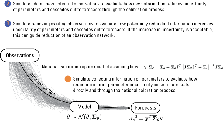
Diagram showing the three main ways the Schur Complement is used to propagate uncertainty from observations to model parameters and through to model forecasts.
Approach 1.—The first strategy is to evaluate the potential value of gaining better information directly on model parameters. If we consider that the parameters follow a multivariate Gaussian distribution , we can evaluate the contribution of each parameter by repeating the calculations of equation 14 with parameter covariance altered to simulate perfect knowledge of a parameter. This is accomplished by setting the variance of a parameter to zero (setting the diagonal of Σθ corresponding to that parameter to zero) and conditioning the off-diagonal elements to simulate perfect knowledge by reducing the variance of all parameters correlated with the parameter being evaluated proportional to their correlation. The Schur Complement then is used to calculate (for example, the posterior variance with parameter known perfectly). If the parameter is important for the forecast, then will be less than . A metric of parameter importance can be calculated as
Approach 2.—The second strategy is to evaluate the value of potential new observations. This is accomplished by supplementing the Jacobian matrix with a row corresponding to the sensitivity of a potential observation to the parameters. An entry must also be added to the epistemic error covariance matrix (Σϵ) indicating the expected uncertainty of the new observation. Assigning weights to observations—potential or existing—is always somewhat subjective. A common approach for potential new observations is to use the same weight as the best-quality existing observations of a similar type, if they exist, with the logic that new data will be collected using the best techniques available resulting in quality commensurate with the best existing data. The Schur Complement (eq. 15) is used again with the augmented and Σϵ matrices to calculate (the posterior variance with the ith potential observation added), and the importance of the added observation can be calculated by evaluating the decrease in forecast variance with the added observation as
Approach 3.—The third strategy is to evaluate the value of existing observations based on their contribution to forecast uncertainty. This is accomplished by setting the weight of an observation to evaluate to zero on the diagonal of the epistemic error covariance matrix (Σϵ) and then calculating (the posterior variance with the ith observation omitted) using the Schur Complement (eq. 15). The importance of the existing observation can be calculated by evaluating the increase in forecast variance with a removed observation as
Results of Analysis in the Mississippi Alluvial Plain Using Linear Uncertainty Methods
We show the use of linear uncertainty methods in the three approaches described in section “Linear Uncertainty Methods—Three Main Approaches” using the forecast of drawdown at multiple future times in the Sunflower region as the forecast of interest. Haugh and others (2020a) documented a specific region of significant drawdown (referred to in Haugh and others, 2020a, 2020b, and in this work as the “composite hydrograph area”) and various potential remedies to stop or reverse the drawdown. The forecasts of how these remedies might be effective was simulated using the improved Mississippi Embayment Regional Aquifer Study (MERAS) MODFLOW (Hunt and others, 2021) model, which updated the original MODFLOW–2005 (Harbaugh, 2005) version of the model (Clark and others, 2013). In this work, a further update of the MODFLOW model (Hunt and others, 2021), implemented in MODFLOW–NWT (Niswonger and others, 2011), was used to make the same forecasts. The composite hydrograph area, delineating the area over which the forecast is defined, is shown in figure 2.
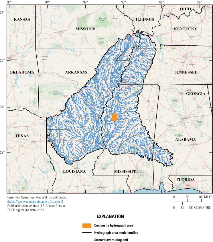
Map showing location of the composite hydrograph area within the Mississippi Embayment Regional Aquifer Study model footprint, Arkansas, Missouri, Illinois, Kentucky, Louisiana, Mississippi, and Alabama.
The updated MODFLOW–NWT model uses 16 stress periods for parameter estimation. An initial 9-year dynamic-equilibrium stress period, representing average stresses from 1998 to 2007, is followed by 15 additional 6-month stress periods. These 15 additional stress periods each represent 6 months and alternate between growing and non-growing seasons. A 50-year forecast period then follows this parameter estimation period with 100 repeated alternating growing and non-growing season 6-month stress periods selected from the parameter estimation time (stress periods 7 and 12 for growing and nongrowing, respectively) resulting in a 50-year forecast period consistent with (Haugh and others, 2020a).
To evaluate data worth, the forecast of interest was identified as the mean drawdown in the composite hydrograph area (refer to fig. 2) at stress periods 17, 37, 57, and 107, representing 0, 10, 20, and 45 years into the simulated forecast period.
To evaluate potential observations, a network of potential head observation locations was simulated at the first stress period of the forecast period (stress period 17). The data worth of these potential observations is discussed in the “Worth of Potential New Observations on Reducing Forecast Uncertainty” section.
The most basic calculation to be made using linear uncertainty methods is the reduction in uncertainty of the forecast prior to parameter estimation with the available dataset and after parameter estimation (the prior and posterior standard deviation, respectively). The prior standard deviation (σ) was 3,367.59 feet and the posterior σ was 0.10 foot. The remainder of this section examines how information on parameters and observations play important roles in contributing to the posterior σ.
Contribution of Parameters to Forecast Uncertainty—Parameter Importance
The first analysis result shows the contribution of various model parameters to uncertainty. This result can be summarized by group to help indicate which broad categories of parameter information contribute most significantly to the posterior uncertainty. As shown in figure 3, recharge pilot points in aggregate (rpp) are the most important, followed by specific yield (sy), anisotropy (aniso), and horizontal hydraulic conductivity pilot points in aggregate (hkpp). The remaining parameter groups include zones of hydraulic conductivity (horizontal and vertical), streamflow routing (sfr), and specific storage (ss).
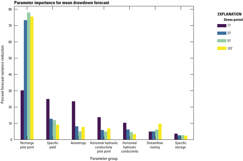
Bar graph showing parameter importance (eq. 16) aggregated to each parameter group. Individual bars correspond with specific stress periods in the model.
Worth of Existing Observations on Reducing Forecast Uncertainty
The worth of existing observations can be calculated using equation 18. This has the dual purpose of potentially helping indicate which observations may be redundant in a monitoring network and helping users to understand the importance of specific observations in the calibration dataset as they impact forecast uncertainty. Figure 4 shows the locations of the observations scaled by their removed observation importance, aggregated across all stress periods. The “x” marks on figure 4 indicate all locations of head observations that were available for at least part of the history-matching time period. Two forecasts were evaluated for this analysis—the mean and median drawdown in the composite hydrograph area. In figure 4A and 4B showing aggregated data worth for both forecasts, the colored circle symbols indicate aggregated normalized data worth for all existing observation locations with a value greater than 0.001. The aggregated normalized data worth was calculated by summing the calculated data worth across all forecast and history-matching stress periods for which an observation was simulated at each specific location. This quantity was then normalized by dividing by the maximum aggregated value at each point. Therefore, the actual magnitude of the quantity does not have an interpretable value, but the relative rank of the values can help inform which locations have relatively more or less value. As figure 4A and 4B indicates, the patterns are not well connected with hydrologic features such as the streamflow routing (sfr) cells. Indeed, although the highest value in each case is near the composite hydrograph area, it is not within the area, which is suspicious. The density of existing data confounds the ability of this analysis to identify a single most important or valuable data point. The level of redundancy of existing data indicates that, in this case, the analysis does not deeply inform decisions to remove data from future consideration.
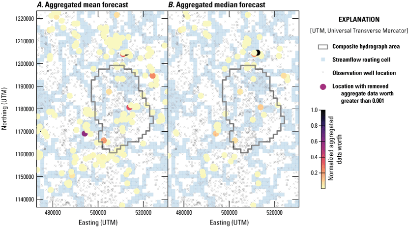
Images showing aggregated data worth for removed, existing observation locations across all stress periods. A, Aggregated mean drawdown forecast. B, Aggregated median drawdown forecasts.
Worth of Potential New Observations on Reducing Forecast Uncertainty
The final analysis using linear uncertainty methods evaluated the contributions to uncertainty reduction made by data obtained from new observations. For this evaluation, a network of potential head observations was simulated in every model cell within a buffer of about 10 miles around the composite hydrograph area. Despite good spatial coverage of head observations used for the calibration of the model, this exercise was performed to evaluate the potential to fill in gaps of unobserved areas and to focus on data collected at the onset of the forecast period. Forecast uncertainty was evaluated at each stress period (for example, 6-month intervals) for the entire 50-year forecast period. As discussed in the “First-Order Second-Moment (FOSM) Propagation of Variance” section, data worth must be evaluated with respect to a specific forecast of interest. As a result, potential data worth values exist for every simulated potential observation location for all 100 forecast-period stress periods. An aggregated representation of data worth, normalized to the maximum aggregated data worth over all forecast time, is shown in figure 5A. In other words, the scale from 0.0 to 1.0 is intended to convey the spatial location of maximum forecast uncertainty reduction achieved if a new head observation is made at the beginning of the forecast period (stress period 17). A heatmap of the typical location of the maximum drawdown within the composite hydrograph area, to provide some context regarding where most additional information is likely to be found if adding a new observation, is shown in figure 5B. The actual decrease of forecast variance for the mean drawdown is shown in figure 5C and generally decreases throughout the forecast time. This trend highlights that, as time continues in the forecast period, the value of monitoring new data decreases because more of the actual forecast time has elapsed and monitoring data at the beginning of the forecast period is eclipsed by actual observations throughout that time period. These results show that potential new data are most valuable close to the center of mass of where the maximum drawdown forecast is located. This conclusion is logical, as pumping greater than recharge is the key driver of drawdown, so collecting more data in the region where the forecast is occurring should be informative about the forecast. Observations at the beginning of the forecast period are also more informative than subsequent observations as the forecast period elapses (fig. 5C). The evolution of the actual forecast over time and that, once the trajectory is underway, the value of observations at the beginning of the forecast period diminishes, are shown in figure 5D.
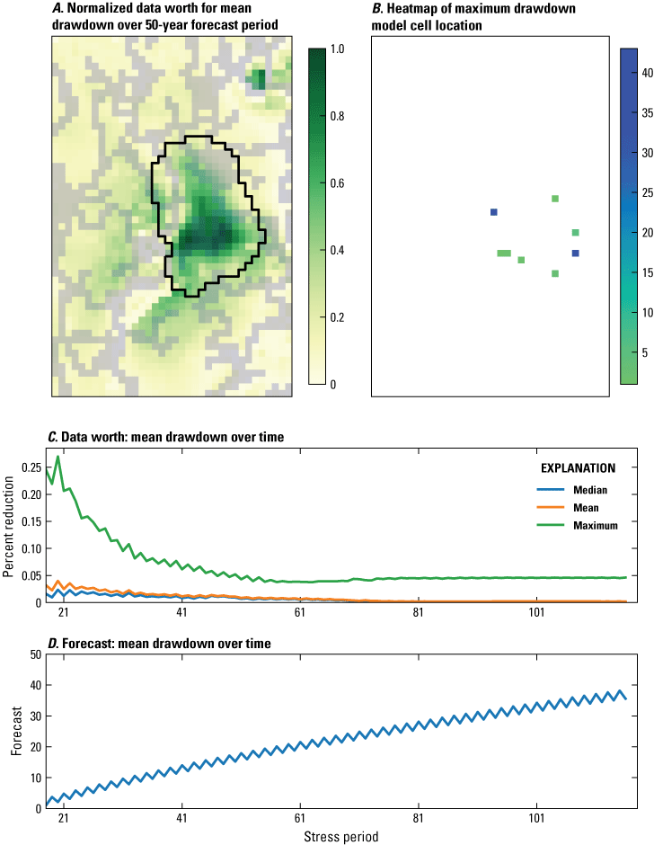
Image, heatmap, and graphs showing value of potential new observations, collected at the end of the history-matching period with importance aggregated over all future time. A, Aggregated representation of data worth, normalized to the maximum aggregated data worth over 50-year forecast period. B, Maximum drawdown model cell location. C, Data worth—mean drawdown over time. D. Actual forecast—mean drawdown over time.
Limitations and Lessons Learned
We have described the theoretical background and provided an example of use of a groundwater-flow model for evaluating data worth using a parameter-estimation mathematical and statistical framework. The metric of uncertainty of a forecast of interest is the key metric with which to judge data worth.
Limitations
The mathematical framework depends on the Jacobian matrix, a prior covariance structure for the parameters, and a meaningful observation weighting scheme. All of these elements depend on a model that is stable, predictable in its behavior, and a reasonable simulator of the system. Instabilities and large misrepresentations of the system dynamics can negatively impact the value of data-worth calculations.
Summary, Conclusions, and Lessons Learned
In the example we evaluated, the existence of a large spatially and temporally distributed observation network masks the value of the analysis. For example, the identification of a single observation among hundreds of existing observations as less valuable implies that the information such an observation provides is redundant or disconnected from the forecast of interest. However, with such uniform coverage, one could argue that almost all the observations are redundant and picking one or more to drop is difficult either qualitatively or using the quantitative methods examined here. Similarly, when there are few spatial gaps where observations do not exist, it is difficult for the method to evaluate where additional information could be added. Finally, the temporal aspect of this modeling effort required summarizing observation acquisition and forecast times in ways that make the base units of the data worth quantities difficult to interpret, but instead focus on the rank of data worth from one location to another. The data worth methods presented are perhaps most valuable when fewer observations already exist. Nonetheless, the insights gained are valuable and the low incremental computational cost when a parameter estimation framework is in place make this a valuable analysis tool to use.
References Cited
Clark, B., Westerman, D., and Fugitt, D., 2013, Enhancements to the Mississippi Embayment Regional Aquifer Study (MERAS) groundwater-flow model and simulations of sustainable water-level scenarios: U.S. Geological Survey Scientific Investigations Report 2013–5161, 29 p., accessed February 1, 2025, at https://doi.org/10.3133/sir20135161.
Doherty, J.E., Hunt, R.J., and Tonkin, M.J., 2011, Approaches to highly parameterized inversion—A guide to using PEST for model-parameter and predictive-uncertainty analysis: U.S. Geological Survey Scientific Investigations Report 2010–5211, 71 p. [Also available at https://doi.org/10.3133/sir20105211.]
Doherty, J., and Welter, D., 2010, A short exploration of structural noise: Water Resources Research 46, no. 5, 14 p., accessed February 1, 2025, at https://doi.org/10.1029/2009wr008377.
Fienen, M.N., Doherty, J.E., Hunt, R.J., and Reeves, H.W., 2010, Using prediction uncertainty analysis to design hydrologic monitoring networks—Example applications from the Great Lakes water availability pilot project: U.S. Geological Survey Scientific Investigations Report 2010–5159, 44 p. [Also available at https://doi.org/10.3133/sir20105159.]
Fienen, M.N., White, J.T., and Hayek, M., 2024, Parameter ESTimation with the Gauss–Levenberg–Marquardt Algorithm—An intuitive guide: Groundwater, v. 63, no. 1, p. 1–12, accessed February 1, 2025, at https://doi.org/10.1111/gwat.13433.
Harbaugh, A.W., 2005, MODFLOW-2005—The U.S. Geological Survey modular ground-water model—The ground-water flow process: U.S. Geological Survey Techniques and Methods, book 6, chap. A16, [variously paged]. [Also available at https://doi.org/10.3133/tm6A16.]
Haugh, C.J., Killian, C.D., and Barlow, J.R.B., 2020b, MODFLOW-2005 model used to evaluate water-management scenarios for the Mississippi Delta: U.S. Geological Survey data release, accessed February 1, 2025, at https://doi.org/10.5066/P9906VM5.
Haugh, C.J., Killian, C.D., and Barlow, J.R.B., 2020a, Simulation of water-management scenarios for the Mississippi Delta: U.S. Geological Survey Scientific Investigations Report 2019–5116, 15 p., accessed February 1, 2025, at https://doi.org/10.3133/sir20195116.
Hunt, R.J., White, J.T., Duncan, L.L., Haugh, C.J., and Doherty, J., 2021, Evaluating lower computational burden approaches for calibration of large environmental models: Groundwater, v. 59, no. 6, p. 788–798, accessed February 1, 2025, at 10.1111/gwat.13106.
Nielsen, M.G., and Westenbroek, S.M., 2023, Updated estimates of water budget components for the Mississippi embayment region using a Soil-Water-Balance model, 2000–2020: U.S. Geological Survey Scientific Investigations Report 2023–5080, 58 p., accessed February 1, 2025, at https://doi.org/10.3133/sir20235080.
Niswonger, R.G., Panday, S., and Ibaraki, M., 2011, MODFLOW-NWT, a newton formulation for MODFLOW-2005: U.S. Geological Survey Techniques and Methods, book 6, chap. A37, 44 p., accessed February 1, 2025, at https://doi.org/10.3133/tm6A37.
Welter, D.E., Doherty, J.E., Hunt, R.J., Muffels, C.T., Tonkin, M.J., and Schreüder, W.A., 2012, Approaches in highly parameterized inversion–PEST++, a parameter ESTimation code optimized for large environmental models: U.S. Geological Survey Techniques and Methods, book 7, chap. C5, 47 p. [Also available at https://doi.org/10.3133/tm7C5.]
White, J.T., Doherty, J.E., and Hughes, J.D., 2014, Quantifying the predictive consequences of model error with linear subspace analysis: Water Resources Research, v. 50, no. 2, p. 1152–1173, accessed February 1, 2025, at https://doi.org/10.1002/2013WR014767.
White, J.T., Fienen, M.N., and Doherty, J.E., 2016, A python framework for environmental model uncertainty analysis: Environmental Modelling & Software, v. 85, p. 217–228, accessed February 1, 2025, at https://doi.org/10.1016/j.envsoft.2016.08.017.
White, J. T., Hunt, R.J., Fienen, M.N., and Doherty, J.E., 2020, Approaches to highly parameterized inversion—PEST++ Version 5, a software suite for parameter estimation, uncertainty analysis, management optimization and sensitivity analysis: U.S. Geological Survey Techniques and Methods, book 7, chap. C26, 52 p., accessed February 1, 2025, at https://doi.org/10.3133/tm7C26.
For more information about this publication, contact:
Director, USGS Upper Midwest Water Science Center
8505 Research Way
Middleton, WI 53562
608–828–9901
For additional information, visit: https://www.usgs.gov/centers/umid-water
Publishing support provided by the
Rolla and Tacoma Publishing Service Centers
Disclaimers
Any use of trade, firm, or product names is for descriptive purposes only and does not imply endorsement by the U.S. Government.
Although this information product, for the most part, is in the public domain, it also may contain copyrighted materials as noted in the text. Permission to reproduce copyrighted items must be secured from the copyright owner.
Suggested Citation
Fienen, M.N., Schachter, L.A., and Hunt, R.J., 2025, A model uncertainty quantification protocol for evaluating the value of observation data: U.S. Geological Survey Scientific Investigations Report 2025–5007, 12 p., https://doi.org/10.3133/sir20255007.
ISSN: 2328-0328 (online)
| Publication type | Report |
|---|---|
| Publication Subtype | USGS Numbered Series |
| Title | A model uncertainty quantification protocol for evaluating the value of observation data |
| Series title | Scientific Investigations Report |
| Series number | 2025-5007 |
| DOI | 10.3133/sir20255007 |
| Publication Date | March 17, 2025 |
| Year Published | 2025 |
| Language | English |
| Publisher | U.S. Geological Survey |
| Publisher location | Reston, VA |
| Contributing office(s) | Upper Midwest Water Science Center |
| Description | vi; 12 p. |
| Online Only (Y/N) | Y |
| Additional Online Files (Y/N) | N |