

Hydrogeologic Investigation, Framework, and Conceptual Flow Model of the Antlers Aquifer, Southeastern Oklahoma, 1980–2022
Links
- Document: Report (41 MB pdf) , HTML , XML
- Dataset: USGS National Water Information System database - USGS water data for the Nation
- Data Release: USGS Data Release - Soil-water-balance model and data used in the hydrogeologic investigation, framework, and conceptual flow model of the Antlers aquifer, southeastern Oklahoma, 1967–2022
- NGMDB Index Page: National Geologic Map Database Index Page (html)
- Download citation as: RIS | Dublin Core
Acknowledgments
The authors value the contributions of the Oklahoma Water Resources Board staff that led to the successful completion of this report, especially Christopher Neel (Division Chief, Water Rights Administration Division) and Derrick Wagner (Technical Studies Manager, Water Rights Administration Division), who provided hydrogeologic data and helped with defining study objectives and deliverables. The authors also thank Oklahoma Water Resources Board employees Harold Robertson, Zach McKinney, Anthony Huey, Jason Shiever, Tucker McCoy, Jeremy Colburn, Byron Waltman, and Jon Sanford, who assisted in collecting synoptic water table-altitude measurements.
The authors express gratitude to U.S. Geological Survey employees who performed data-collection activities in the field, especially Steve Smith, Nick Pierson, Kevin Smith, Kyle Cothren, and Levi Close who measured synoptic base flows during 2023. The authors also thank U.S. Geological Survey employees David S. Wallace, Andrew P. Teeple, and Scott J. Ikard, who performed detailed technical reviews on this report and the accompanying data release. The authors acknowledge and appreciate the professionalism, experience, and dedication of these helpful and resourceful colleagues.
Abstract
The 1973 Oklahoma Groundwater Law (Oklahoma Statute §82–1020.5) requires that the Oklahoma Water Resources Board conduct hydrologic investigations of the State’s groundwater basins to support a determination of the maximum annual yield for each groundwater basin. Every 20 years, the Oklahoma Water Resources Board is required to update the hydrologic investigation on which the maximum annual yield determinations were based. The maximum annual yield allocated per acre of land is used to set the equal-proportionate share pumping rate. The maximum annual yield of 5,913,600 acre-feet per year and equal-proportionate-share of 2.1 acre-feet per acre per year currently (2025) in place for the Antlers aquifer were issued by the Oklahoma Water Resources Board on February 14, 1995. Because more than 20 years have elapsed since the 1995 final order for the Antlers aquifer was issued, the U.S. Geological Survey, in cooperation with the Oklahoma Water Resources Board, completed an in-depth hydrologic study that included a hydrogeologic framework and conceptual groundwater-flow model for the 1980–2022 study period.
The results of an analysis of land use, long-term climate patterns, streamflow and base-flow patterns, historical groundwater use, as well as groundwater-level fluctuations across the Antlers aquifer are described. In addition, groundwater quality was analyzed for total dissolved solids concentrations and major ions for the Antlers aquifer. An updated hydrogeologic framework was developed that included refining the aquifer boundary in Oklahoma, the creation of new potentiometric surface and saturated thickness of fresh groundwater maps, one multiple-well aquifer test, slug tests, and an analysis of lithologic logs across the aquifer. A conceptual groundwater flow model and water budget were developed by incorporating estimates of recharge from precipitation, saturated-zone evapotranspiration, streambed seepage, lateral groundwater flows, vertical leakage, and withdrawals from groundwater wells.
Introduction
The 1973 Oklahoma Groundwater Law (Oklahoma Statute §82–1020.5 [Oklahoma State Legislature, 2021a]) requires that the Oklahoma Water Resources Board (OWRB) conduct periodic hydrologic investigations of the State’s aquifers (called groundwater basins in the statutes) to support a determination of the maximum annual yield (MAY) for each aquifer. In Oklahoma, the MAY is defined as the amount of fresh groundwater (groundwater with a total dissolved solids [TDS] concentration of less than 5,000 milligrams per liter [mg/L]) that can be withdrawn annually while ensuring a minimum 20-year life of the aquifer (OWRB, 2012, 2023a, c). TDS is commonly used by many agencies to refer to the concentration of dissolved solids in water and is referred to as such by the OWRB. For bedrock aquifers, the groundwater-basin-life requirement is satisfied if, after 20 years of MAY withdrawals, 50 percent of the groundwater basin (hereinafter referred to as an “aquifer”) retains a saturated thickness of at least 15 feet (ft). Although 20 years is the minimum required by law, the OWRB can and often does consider multiple management scenarios. The annual volume of water allocated to a given groundwater permit applicant is determined once a MAY has been established and is dependent on the amount of land owned or leased by a permit applicant. The MAY is divided by the total land area overlying the aquifer to determine the annual volume of groundwater allocated per acre of land, or the equal-proportionate-share (EPS) pumping rate.
Every 20 years, the OWRB is statutorily required to update the hydrologic investigation on which the maximum annual yield determinations were based. Because more than 20 years have elapsed since the February 14, 1995, final order for the Antlers aquifer was issued, the 1973 Oklahoma Water Law requires the OWRB to reevaluate and update the MAY and EPS pumping rates for the aquifer (Oklahoma State Legislature, 2021b).
The Antlers aquifer in Oklahoma is equivalent to the Trinity aquifer in Texas and Arkansas. The Trinity aquifer (including the part in Oklahoma referred to as the “Antlers aquifer”) is a large aquifer that underlies an area of about 26,240,000 acres, extending from south-central Texas through southeastern Oklahoma before terminating in western Arkansas (fig. 1) (Ryder, 1996; OWRB, 2024).
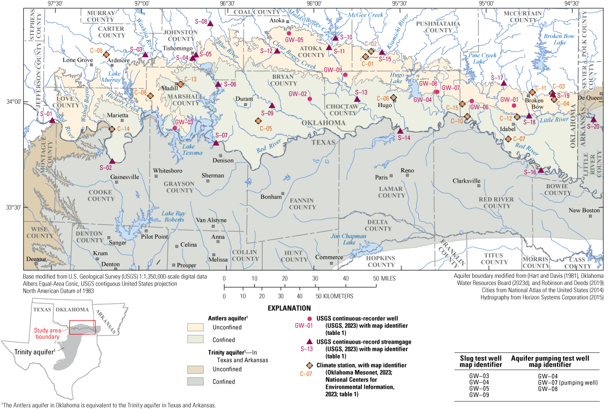
Selected data-collection stations in the Antlers aquifer study area, southeastern Oklahoma, northeastern Texas, and southwestern Arkansas.
The MAY and EPS for the Antlers aquifer were last updated in 1995. The MAY allocated per acre of land is used to set the equal-proportionate share pumping rate. As part of a February 14, 1995, final order, a MAY of 5,913,600 acre-feet per year (acre-ft/yr) and an EPS of 2.1 acre-feet per acre per year (acre-ft/acre/yr) were issued by the OWRB. Because more than 20 years have elapsed since the 1995 final order was issued, the U.S. Geological Survey, in cooperation with the OWRB, developed a hydrogeologic framework and conceptual model to reevaluate the hydrogeologic properties of the Antlers aquifer. The effects of potential groundwater withdrawals on groundwater flow and availability were also evaluated during the 1980–2022 study period to help provide OWRB with the information needed for updating the MAY and EPS pumping rates for the aquifer. The MAY and EPS pumping rates currently in place were determined from the hydrologic investigations of the Antlers aquifer done by Hart and Davis (1981) and Morton (1992). Morton (1992) used a numerical groundwater-flow model to evaluate the effects of potential groundwater withdrawals on the availability of groundwater in the Antlers aquifer in southeastern Oklahoma.
Purpose and Scope
The purpose of this report is to (1) provide an updated summary of the hydrogeology and hydrogeologic framework of the Antlers aquifer in southeastern Oklahoma (including an updated geographic extent), and (2) describe the development of a conceptual groundwater-flow model representing the period 1980–2022 as part of the hydrologic investigation. Parts of the equivalent Trinity aquifer in northeastern Texas and southwestern Arkansas were included in the analyses of aquifer properties that could influence groundwater availability in the Antlers aquifer; however, the focus of the hydrologic investigation described in this report was the Antlers aquifer in southeastern Oklahoma.
Description of Antlers Aquifer Study Area
The rocks that contain the Antlers aquifer cover all or part of Atoka, Bryan, Carter, Choctaw, Johnston, Love, Marshall, McCurtain, and Pushmataha Counties in southeastern Oklahoma (fig. 1). As explained in the first part of the “Introduction” section of this report, the Antlers aquifer is equivalent to the Trinity aquifer in Texas and Arkansas. The rocks that contain the Trinity aquifer in the northeastern part of Texas and the southeastern part of Arkansas are part of the study area (fig. 1).
The Antlers aquifer is contained in Cretaceous bedrock (Hart and Davis, 1981; OWRB, 2012) and is unconfined in an approximately 3- to 15-mile (mi)-wide band that extends westward from the Oklahoma-Arkansas border to Marietta, Oklahoma, where the generally east-west surficial exposure of the rocks that contain the aquifer in Oklahoma and Arkansas extends southward into Texas (fig. 1; Hart and Davis, 1981). The Antlers aquifer is confined to the south and east of the outcrop area. The larger, confined part of Antlers aquifer is downgradient from the smaller, unconfined part of the aquifer, including the large, confined part of the aquifer that extends into Texas. Several streams overlie the Antlers aquifer, including the Red River and major tributaries including the Blue River, Kiamichi River, Little River, Clear Boggy Creek, Muddy Boggy Creek, and the Washita River (fig. 1). Where these streams overlie the unconfined part of the Antlers aquifer, alluvium and terrace deposits are hydrologically connected to the Antlers aquifer.
Land Use
Land-use data at a resolution of 30 meters (m) overlying the Antlers aquifer were obtained from the CropScape database for 2022 (figs. 2–3; National Agricultural Statistics Service, 2023; U.S. Department of Agriculture [USDA], 2024). Land cover overlying the unconfined part of the Antlers aquifer was primarily forest/shrubland (48.4 percent) and grass/pastures (37.1 percent) (figs. 2, 3B). The remaining land was developed (4.2 percent), cropland (2.2 percent), and other types (8.1 percent) (fig. 3B) which included open water, wetlands, and barren land. Cropland accounted for most of the land cover near the Red River at the Oklahoma-Texas border (fig. 2). The most prominent crops grown on top of the unconfined part of the Antlers aquifer included hay and alfalfa, winter wheat, soybeans, corn, and cotton (44.4, 34.2, 4.2, 1.8, and 0.2 percent, respectively, of the total cropland in the unconfined part of the aquifer); fallow and idle land also accounted for 0.7 percent of total cropland in the unconfined part of the Antlers aquifer (fig. 3B; National Agricultural Statistics Service, 2023; USDA, 2024). Various other crops (14.5 percent) were also present over the unconfined part of the Antlers aquifer, but in much smaller quantities comparatively. It should be noted that crop types may change throughout the year and from year to year with seasonal, economic, and hydrologic factors.

Land and cropland cover types in the Antlers aquifer study area, southeastern Oklahoma, 2022.

A, Distribution of land and crop cover types in the Antlers aquifer study area, 2022, and B, distribution of land and crop cover types for the unconfined part of the Antlers aquifer, 2022 (National Agricultural Statistics Service, 2023; U.S. Department of Agriculture [USDA], 2024).
Long-Term Climate Patterns
The Antlers aquifer is in a humid subtropical climate area (Kottek and others, 2006). Daily climate data for 1907–2022 (mean daily precipitation, and minimum, maximum, and mean daily temperatures) were compiled from 15 climate stations in or near the Antlers aquifer study area (fig. 1; table 1; National Centers for Environmental Information [NCEI], 2023; Oklahoma Mesonet, 2023).
Table 1.
Selected data-collection sites in the Antlers aquifer study area, southeastern Oklahoma.[U.S. Geological Survey (USGS, 2023) data can be accessed in the National Water Information System database by using the 8- or 15-digit station number or other identifier. Dates shown as month, day, year. NAD 83, North American Datum of 1983; NAVD 88, North American Vertical Datum of 1988; Ave, avenue; Okla., Oklahoma; Tex., Texas; Ark., Arkansas; SW, southwest; --, unknown or not applicable]
| Station number or identifier (fig. 1) |
Map identifier (fig. 1) |
Station name | Latitude (decimal degrees NAD 83) | Longitude (decimal degrees NAD 83) | Period of record used in the analysis (may contain gaps) | Land-surface altitude (feet above NAVD 88) | Well or hole depth (feet below land surface) | |
|---|---|---|---|---|---|---|---|---|
| Begin | End | |||||||
| 07315650 | S-01 | Red River near Courtney, Okla. | 33.918 | −97.508 | 10/7/2009 | 12/31/2022 | -- | -- |
| 07316000 | S-02 | Red River near Gainesville, Tex. | 33.728 | −97.160 | 10/1/1936 | 12/31/2022 | -- | -- |
| 07331000 | S-03 | Washita River near Dickson, Okla. | 34.233 | −96.976 | 10/1/1928 | 12/31/2022 | -- | -- |
| 07331290 | S-04 | Washita River near Tishomingo, Okla. | 34.219 | −96.702 | 7/21/1953 | 12/31/2022 | -- | -- |
| 07331383 | S-05 | Pennington Creek at Capitol Ave at Tishomingo, Okla. | 34.235 | −96.683 | 12/6/2012 | 12/31/2022 | -- | -- |
| 07331455 | S-06 | Lake Texoma at Cumberland Cut near Cumberland, Okla. | 34.097 | −96.553 | 12/14/2015 | 12/31/2022 | -- | -- |
| 07331600 | S-07 | Red River at Denison Dam near Denison, Tex. | 33.819 | −96.563 | 1/1/1924 | 12/31/2022 | -- | -- |
| 07332390 | S-08 | Blue River near Connerville, Okla. | 34.383 | −96.601 | 9/24/1956 | 12/31/2022 | -- | -- |
| 07332500 | S-09 | Blue River near Blue, Okla. | 33.997 | −96.241 | 6/10/1936 | 12/31/2022 | -- | -- |
| 07333900 | S-10 | McGee Creek Reservoir near Farris, Okla. | 34.316 | −95.875 | 10/1/2003 | 12/31/2022 | -- | -- |
| 07334000 | S-11 | Muddy Boggy Creek near Farris, Okla. | 34.271 | −95.912 | 10/1/1937 | 12/31/2022 | -- | -- |
| 07334800 | S-12 | Clear Boggy Creek above Caney Creek near Caney, Okla. | 34.255 | −96.213 | 10/6/1976 | 12/31/2022 | -- | -- |
| 07335300 | S-13 | Muddy Boggy Creek near Unger, Okla. | 34.027 | −95.750 | 10/18/1961 | 12/31/2022 | -- | -- |
| 07335500 | S-14 | Red River at Arthur City, Tex. | 33.875 | −95.502 | 10/1/1905 | 12/31/2022 | -- | -- |
| 07336200 | S-15 | Kiamichi River near Antlers, Okla. | 34.249 | −95.605 | 9/11/1962 | 12/31/2022 | -- | -- |
| 07336820 | S-16 | Red River near De Kalb, Tex. | 33.684 | −94.694 | 1/3/1968 | 12/31/2022 | -- | -- |
| 07337900 | S-17 | Glover River near Glover, Okla. | 34.098 | −94.902 | 5/13/1968 | 12/31/2022 | -- | -- |
| 07338500 | S-18 | Little River below Lukfata Creek, near Idabel, Okla. | 33.941 | −94.759 | 1/1/1930 | 12/31/2022 | -- | -- |
| 07339000 | S-19 | Mountain Fork near Eagletown, Okla. | 34.042 | −94.620 | 8/18/1915 | 12/31/2022 | -- | -- |
| 07340000 | S-20 | Little River near Horatio, Ark. | 33.919 | −94.387 | 8/1/1915 | 12/31/2022 | -- | -- |
| 335915094504101 | GW-01 | Antlers01 | 33.988 | −94.845 | 11/17/2021 | 12/31/2022 | 419.12 | 56 |
| 340130096012501 | GW-02 | Antlers02 | 34.025 | −96.024 | 11/18/2021 | 12/31/2022 | 620.11 | 400 |
| 335301096480601 | GW-03 | Antlers03 | 33.884 | −96.802 | 11/18/2021 | 3/28/2023 | 654 | 160 |
| 340324095174501 | GW-04 | Antlers04 | 34.057 | −95.296 | 12/13/2021 | 12/31/2022 | 539.26 | 320 |
| 342006096083901 | GW-05 | Antlers06 | 34.335 | −96.144 | 6/14/2022 | 12/31/2022 | 670.30 | 51 |
| 340042095051801 | GW-06 | McCurtain 27 | 34.012 | −95.089 | 1/1/1956 | 12/31/2022 | 552.72 | 120 |
| 340322095173201 | GW-07 | Aquifer test pumping well | 34.057 | −95.293 | 11/16/2022 | 11/21/2022 | 557 | 318 |
| 340322095171501 | GW-08 | Aquifer test observation well | 34.056 | −95.288 | 10/27/2022 | 11/21/2022 | 545 | 323 |
| 340821095490401 | GW-09 | AntlersSlug02 | 34.139 | −95.818 | 3/29/2023 | 3/29/2023 | 465 | 78 |
| ANT2 | C-01 | Antlers | 34.250 | −95.668 | 4/15/2011 | 12/31/2022 | -- | -- |
| ANTL | C-02 | Antlers | 34.224 | −95.701 | 1/1/1994 | 4/14/2011 | -- | -- |
| BBOW | C-03 | Broken Bow | 34.014 | −94.613 | 1/1/1994 | 11/19/2002 | -- | -- |
| BROK | C-04 | Broken Bow | 34.043 | −94.624 | 4/4/2003 | 12/31/2022 | -- | -- |
| DURA | C-05 | Durant | 33.921 | −96.320 | 1/1/1994 | 12/31/2022 | -- | -- |
| HUGO | C-06 | Hugo | 34.031 | −95.540 | 1/1/1994 | 12/31/2022 | -- | -- |
| IDAB | C-07 | Idabel | 33.830 | −94.880 | 1/1/1994 | 12/31/2022 | -- | -- |
| MADI | C-08 | Madill | 34.036 | −96.944 | 1/1/1994 | 12/31/2022 | -- | -- |
| NEWP | C-09 | Newport | 34.228 | −97.201 | 10/3/2002 | 12/31/2022 | -- | -- |
| VALL | C-10 | Valliant | 33.939 | −95.115 | 10/14/2015 | 12/31/2022 | -- | -- |
| Broken Bow | C-11 | Broken Bow, Okla. | 34.050 | −94.738 | 11/1/1917 | 10/11/2021 | -- | -- |
| Idabel | C-12 | Idabel, Okla. | 33.934 | −94.828 | 9/1/1941 | 1/31/2015 | -- | -- |
| Madill | C-13 | Madill, Okla. | 34.092 | −96.771 | 12/1/1936 | 12/31/2022 | -- | -- |
| Marietta | C-14 | Marietta 5 SW, Okla. | 33.876 | −97.164 | 9/1/1937 | 4/16/2021 | -- | -- |
| Valliant | C-15 | Valliant, Okla. | 33.998 | −95.143 | 2/22/1907 | 12/31/2022 | -- | -- |
The mean annual precipitation for the 1980–2022 study period was 45.2 inches per year (in/yr), whereas the mean annual temperature was 62.9 degrees Fahrenheit (°F; NCEI, 2023; Oklahoma Mesonet, 2023). The mean annual precipitation and temperature for the study period differed slightly from the period of record (1907–2022). The mean annual precipitation for the period of record was 43.9 in/yr, whereas the mean annual temperature was 63.4 °F (fig. 4). Precipitation amounts vary from year to year; the lowest annual precipitation for the 1980–2022 study period was 27.7 inches (in.) for 2005, and the highest annual precipitation for the 1980–2022 study period was 72.2 in. for 2015 (fig. 4A; NCEI, 2023; Oklahoma Mesonet, 2023). In general, May is the wettest month, whereas January is the driest; and June, July, and August are the hottest months, whereas December and January are the coldest (fig. 5). There was a substantial increase in precipitation from west to east across the Antlers aquifer. The Marietta climate station (C-14; table 1; fig. 1; NCEI, 2023) in the western extent of the Antlers aquifer received a mean annual precipitation of 36.2 in/yr for the period of record (1938–2020), whereas the Broken Bow climate stations in the eastern extent of the Antlers aquifer (C-03, C-04, and C-11; table 1; fig. 1; NCEI, 2023; Oklahoma Mesonet, 2023) received a mean annual precipitation of 50.2 in/yr for the period of record (1918–2022) (NCEI, 2023; Oklahoma Mesonet, 2023).

A, Annual mean precipitation, and B, annual mean temperature computed from available climate stations in and near the Antlers aquifer study area shown with locally weighted scatterplot smoothing (LOWESS) curves and estimated cool or warm and wet or dry periods for the 1907–2022 period of record, southeastern Oklahoma.
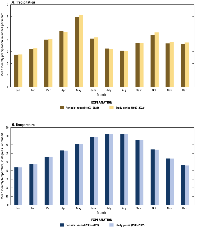
A, Mean monthly precipitation, and B, mean monthly temperature in the Antlers aquifer study area for the period of record (1907–2022) and study period (1980–2022), southeastern Oklahoma (National Centers for Environmental Information [NCEI], 2023; Oklahoma Mesonet, 2023).
Streamflow and Base-Flow Patterns
Streamflow data at selected USGS streamgages in the Antlers aquifer study area (fig. 1) were summarized for the 1980–2022 study period (table 2). Streamflow measured at a point on a stream (or calculated at a streamgage) is the sum of runoff and net base flow originating upstream in the watershed. Base flow is the component of streamflow that is supplied by the discharge of groundwater to streams (Barlow and Leake, 2012). For this report, streamflow-hydrograph data (USGS, 2023) were separated into runoff and base-flow components by using the standard Base-Flow Index (BFI) code (Wahl and Wahl, 1995) included in the USGS Groundwater Toolbox (Barlow and others, 2015). In the BFI code, the minimum streamflow in a moving n-day window serves as the basis for hydrograph separation, where n is the user-defined number of days. Turning points for defining the base-flow hydrograph are then determined by selecting the minimum n-day value that is less than adjacent n-day minimum values on the base flow hydrograph when multiplying by 0.9 (called the user-defined f-statistic). Moix and Galloway (2005, p. 2) explain “minimums [minimum n-day values] are compared to adjacent minimums to determine turning points on the base-flow hydrograph. If 90 percent of a given minimum is less than both adjacent minimums, then that minimum is a turning point. Straight lines are drawn between the turning points to define the base-flow hydrograph.” Base flows were linearly interpolated between the selected turning points and aggregated to the desired monthly temporal resolution. Multiple n-day bins were tested by plotting mean BFI (percentage of streamflow that is classified as base flow) against the n-day value and looking for a reduction in slope. For consistency, a 5-day window and an f-statistic of 0.9 were used for all streamgages in this report.
Table 2.
Mean annual streamflow and base flow for the period of record at selected U.S. Geological Survey (USGS) streamgages (various years during 1925–2020) and for the study period (1980–2022) in southeastern Oklahoma.[USGS values computed by using the Base-Flow Index code (Wahl and Wahl, 1995) in the USGS Groundwater Toolbox (Barlow and others, 2015); acre-ft/yr, acre-foot per year; POR, period of record]
| USGS streamgage number (table 1) | Map identifier (fig. 1) | Mean annual streamflow,1 1980–2022 study period (thousands of acre-ft/yr) | Mean annual base flow,1 1980–2022 study period (thousands of acre-ft/yr) | Mean annual streamflow,1 POR (thousands of acre-ft/yr) | Mean annual base flow,1 POR (thousands of acre-ft/yr) | POR1 |
|---|---|---|---|---|---|---|
| 07316000 | S-02 | 2,545.9 | 905.9 | 2,250.3 | 713.1 | 1937–2022 |
| 07332390 | S-08 | 93.0 | 54.0 | 88.8 | 52.2 | 1977–78; 2004–22 |
| 07332500 | S-09 | 254.3 | 74.8 | 234.4 | 66.8 | 1937–2022 |
| 07334000 | S-11 | 647.1 | 105.9 | 647.2 | 76.1 | 1938–2022 |
| 07334800 | S-12 | 434.6 | 94.5 | 434.6 | 94.5 | 2013–22 |
| 07335300 | S-13 | 1,385.5 | 302.5 | 1,385.5 | 302.5 | 1983–2022 |
| 07337900 | S-17 | 382.8 | 67.1 | 366.3 | 63.8 | 1962–2022 |
| 07338500 | S-18 | 1,354.5 | 450.8 | 1,285.8 | 380.7 | 1947–2022 |
| 07339000 | S-19 | 1,063.8 | 236.7 | 996.2 | 221.7 | 1925; 1930–2022 |
| 07340000 | S-20 | 3,061.0 | 1,238.9 | 2,900.7 | 968.8 | 1932–2022 |
Data from USGS National Water Information System (USGS, 2023).
Although many USGS streamgages were located in the study area, only USGS streamgage 07334800 Clear Boggy Creek above Caney Creek near Caney, Okla. (map identifier S-12) (hereinafter referred to as the “Caney Creek streamgage”) and USGS streamgage 07338500 Little River below Lukfata Creek, near Idabel, Okla. (map identifier S-18) (hereinafter referred to as the “Lukfata Creek streamgage”) overlie the unconfined part of the Antlers aquifer (fig. 1; tables 1–2). The long periods of record for the Caney Creek and Lukfata Creek streamgages are ideal for analyzing the relation between streamflow and base flow. Base flows at the Caney Creek streamgage were computed by applying the BFI method (Wahl and Wahl, 1995) to streamflow data collected during 2013–22; the computed base flows were relatively stable over this period (fig. 6A). Base flows at the Lukfata Creek streamgage were also computed from 1947 to 2022 by using the BFI method, and the base flows at this gage were relatively stable over this period (fig. 6B; USGS, 2023). For their periods of record within the 1980–2022 study period, the mean BFI values for the Caney Creek (map identifier S-12) and Lukfata Creek (map identifier S-18) streamgages were 21.7 percent and 33.3 percent of the mean streamflow, respectively, and 21.7 percent and 29.6 percent of the streamflow, respectively, for their complete periods of record (table 2). Compared to infrequent, intense storms that generate large amounts of surface runoff, more frequent storms with slower precipitation rates typically result in more precipitation infiltrating the ground and reaching the water table as recharge (Sophocleous and Buchanan, 2003).

Annual mean streamflow, base flow, Base-Flow Index, and runoff component of streamflow for A, U.S. Geological Survey (USGS) streamgage 07334800, Clear Boggy Creek above Caney Creek near Caney, Oklahoma (map identifier S-12; table 1), and B, USGS streamgage 07338500 Little River below Lukfata Creek, near Idabel, Okla. (map identifier S-18; table 1), southeastern Oklahoma.
Groundwater Levels in the Antlers Aquifer
Continuous water-level recorders were installed in six preexisting wells completed in the Antlers aquifer. Equipment was installed in one well (GW-06) in 2013, in four wells (GW-01, GW-02, GW-03, and GW-04) in 2021, and in one well (GW-05) in 2022 (fig. 1; table 1) as part of the investigation described in this report. The continuous water-level recorder installed in well GW-03 was removed in 2023 after recording data indicative of lake-level fluctuations instead of groundwater fluctuations because of its proximity to Lake Texoma (fig. 1). The continuous water-level recorder in well GW-05 was not installed until June 2022 and had periods of missing data; thus, the data were not adequate to be included in the analyses for this report. Patterns observed in the remaining four wells indicate that groundwater levels fluctuate throughout the year in the Antlers aquifer and typically increase during spring and fall and decrease during summer and winter (fig. 7). Wells GW-01 and GW-06 are completed in the unconfined part of the Antlers aquifer (fig. 1) and show groundwater-level changes in response to precipitation (fig. 7A–B). Although well GW-02 is completed in the confined part of the aquifer (fig. 1), it also shows groundwater-level changes in response to precipitation (fig. 7C). No continuous water-level recorders were installed in existing wells in the western part of the Antlers aquifer owing to the small number of suitable wells where well access and landowner permission could be obtained. The continuous water-level recorder wells were used to aid in estimating recharge and leakage, which is discussed further in the “Conceptual Groundwater Flow Model and Water Budget” section of this report.
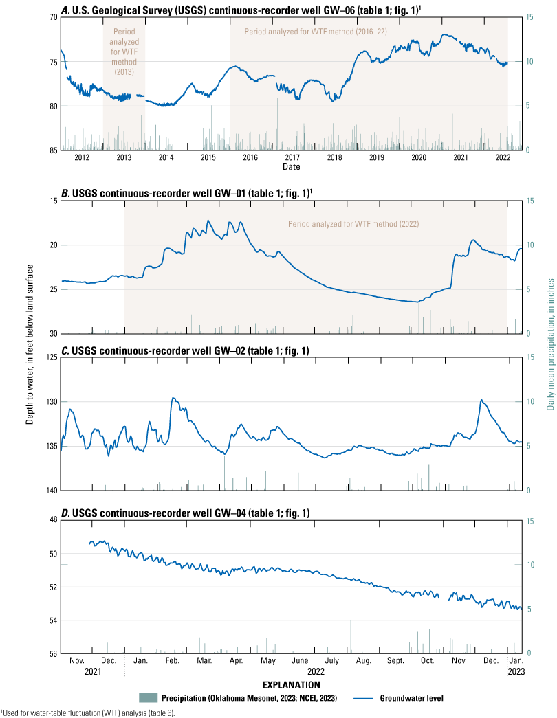
Groundwater-level data for the Antlers aquifer obtained from U.S. Geological Survey (USGS) continuous water-level recorder wells A, GW-06; B, GW-01; C, GW-02; and D, GW-04, along with daily mean precipitation for the study area, southeastern Oklahoma, 2013–22. The periods of record used for water-table fluctuation method from USGS continuous-recorder wells GW-06 and GW-01 are identified. NCEI, National Centers for Environmental Information.
Groundwater Use
The OWRB permits and regulates groundwater use of more than 5 acre-ft/yr for domestic use and requires the annual self-reporting of domestic uses that exceed this threshold. OWRB explains domestic use as follows:
Domestic use includes the use of water for household purposes, farm and domestic animals up to the normal grazing capacity of the land, and the irrigation of land not exceeding a total of three acres in area for the growing of gardens, orchards, and lawns. Domestic use also includes water used for agricultural purposes by natural individuals, use for fire protection, and use by non-household entities for drinking water, restrooms, and watering of lawns, provided such uses do not exceed five acre-feet per year (OWRB, 2025, p. 1).
Other groundwater uses are self-reported annually to the OWRB under the categories of irrigation, public supply, industrial, power, mining, commercial, agricultural, recreation, and fish and wildlife (Oklahoma Statute §82–1020.1[2] [Oklahoma State Legislature, 2021b, c; Oklahoma Statute §82–1020.3 [Oklahoma State Legislature, 2021c]). The Antlers aquifer is used primarily for municipal, irrigation, and industrial supply in Oklahoma (figs. 8–10; tables 3–4; OWRB, 2012). In Texas, withdrawals from the equivalent Trinity aquifer are used primarily for irrigation (Ashworth and Hopkins, 1995; George and others, 2011). In Oklahoma, large capacity wells completed in the Antlers aquifer are capable of yielding 100–500 gallons per minute; however, groundwater withdrawals from large capacity wells are generally minimal because of a reliance on surface-water supply (OWRB, 2012). Groundwater permit holders in Oklahoma have been required to submit annual groundwater-use reports since 1967, and irrigation groundwater-use amounts were based on crop type, acreage, and frequency of application. In 1980, the method was updated to include inches of groundwater applied to increase accuracy of the estimated irrigation groundwater use (OWRB, 2023b). Most of the reported groundwater withdrawn from the Antlers aquifer was used for public supply and irrigation (table 3), which together accounted for 77 percent of the total reported groundwater use for the study period. Reported withdrawals for industrial groundwater use (which were mostly concentrated in McCurtain County) were much higher than the mean in recent years (fig. 8; tables 3–4), accounting for 45 percent of all reported groundwater use between 2011 and 2022. Reported groundwater withdrawals for irrigation during 1967–2022 were concentrated in Love County, accounting for approximately 71 percent of all irrigation groundwater use (fig. 10; table 4). Compared to reported irrigation withdrawals, reported groundwater withdrawals for public supply were somewhat more evenly distributed across the study area but were still concentrated in just two counties (Choctaw and Love Counties) (table 4). Reported groundwater-use data are summarized in the companion USGS data release to this report (Fetkovich and others, 2025).

A, Mean annual groundwater use per year depicted by category, and B, annual reported groundwater use, Antlers aquifer, southeastern Oklahoma, 1967–2022.
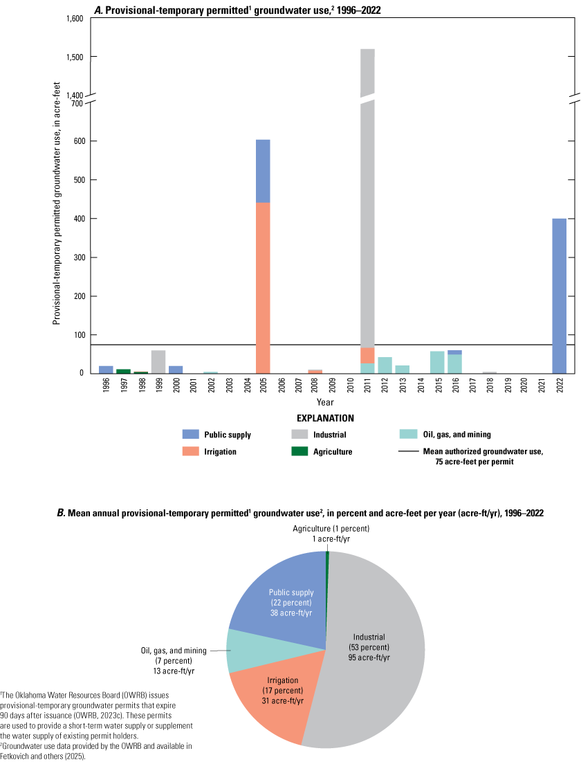
Annual groundwater use authorized for provisional-temporary groundwater-use permits depicted A, as the provisional temporary groundwater use authorized during each year, and B, as the mean annual amount for the entire 1996–2022 period, Antlers aquifer, southeastern Oklahoma, 1967–2022.
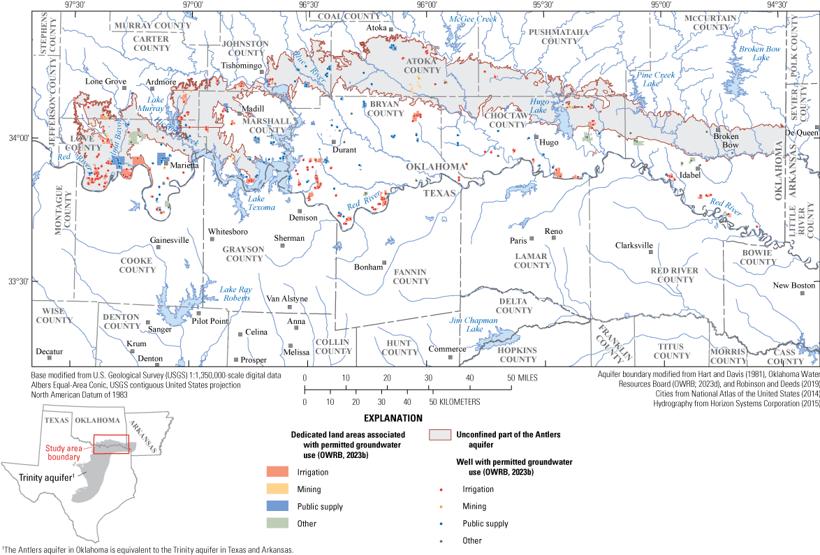
Dedicated land areas and wells permitted for groundwater use from the Antlers aquifer in southeastern Oklahoma, 2023.
Table 3.
Mean annual reported groundwater use by type for the Antlers aquifer, southeastern Oklahoma, 1967–2022.Groundwater use data were provided by the Oklahoma Water Resources Board and are available in an accompanying U.S. Geological Survey data release (Fetkovich and others, 2025).
Table 4.
Mean annual reported groundwater use by type and county for the Antlers aquifer, southeastern Oklahoma, 1967–2022.[<, less than]
Groundwater use data were provided by the Oklahoma Water Resources Board and are available in an accompanying U.S. Geological Survey data release (Fetkovich and others, 2025).
Long-Term Permitted Groundwater Use
A total of 28 of the 125 long-term groundwater permits active in 2022 for the Antlers aquifer were prior-right permits. The OWRB defines a prior-right groundwater permit as the right to use groundwater established by compliance with laws in effect prior to July 1, 1973 (OWRB, 2023c). An additional 29 long-term groundwater permits, 5 of which were prior rights, became inactive in or before 2022 and are also included in a statistical analysis. Mean annual reported groundwater use associated with long-term groundwater permits for the Antlers aquifer was 3,483 acre-ft/yr during the study period (table 5); median annual groundwater use was 2,927 acre-ft/yr during this same period. Public supply accounted for 44 percent of the mean annual reported groundwater use during 1967–2022, followed by irrigation (37 percent), industrial (17 percent), mining (1 percent), with the rest of the use categories together accounting for the remaining 1 percent (fig. 8A).
Table 5.
Summary statistics of annual reported groundwater use for the Antlers aquifer, southeastern Oklahoma, 1967–2022.Groundwater use data were provided by the Oklahoma Water Resources Board and are available in an accompanying U.S. Geological Survey data release (Fetkovich and others, 2025).
Groundwater-use data were also analyzed for four time periods: 1967–80, 1981–2010, 1980–2022, and 2011–22. The reported irrigation groundwater use was generally higher during 1967–80 than during the other time periods, whereas overall groundwater use, especially industrial groundwater use, was generally higher in 1980–2022 and 2011–22 than it was in 1967–80 and 1981–2010 (fig. 8B). The higher reported amounts of irrigation groundwater use pre-1980 may stem from a change in estimation methodology for irrigation amounts by the OWRB; the large increase in industrial groundwater use in 2012 is from a single permit in McCurtain County (table 4), which first reported groundwater use for that year. Mean annual groundwater use was 2,982 acre-ft/yr during 1967–80, 2,706 acre-ft/yr during 1981–2010, 5,429 acre-ft/yr during 2011–22, 3,358 acre-ft/yr during 1967–2022, and 3,483 acre-ft/yr during 1980–2022 (table 3). The median annual groundwater use during 1967–80 was 2,807 acre-ft/yr, which was similar to the median groundwater use during 1981–2010 (2,643 acre-ft/yr), 1967–2022 (2,840 acre-ft/yr), and 1980–2022 (2,927 acre-ft/yr), but differed appreciably from the median groundwater use during 2011–22 (5,202 acre-ft/yr) (table 5). The minimum and maximum annual reported groundwater use totals for 1967–2022 were 945 acre-feet (acre/ft) in 1968 and 8,884 acre-ft in 2016 (table 5; OWRB, 2023b).
For the 125 active long-term groundwater permits issued for the Antlers aquifer, 48,222 acre-ft of groundwater withdrawals were allocated, and 6,675 acre-ft of groundwater use were reported for 2022. The large discrepancy between allocated groundwater withdrawals and reported groundwater withdrawals resulted from permit holders that did not submit a groundwater use report for 2022 and permit holders that reported a groundwater use that was appreciably less than their allocation. There were 14 active permit holders with a right to use more than 1,000 acre-ft/yr of groundwater in 2022, and 6 of these permit holders did not submit groundwater use reports for that year. The remaining eight permit holders reported groundwater use totals that were less than their allocated amount; only one of those permit holders used more than 15 percent of their total allocation. Of all active permit holders with rights to withdraw water from the Antlers aquifer, 59 percent did not report groundwater use in 2022 and 65 percent of those who submitted reports used less than half of their allocation.
Provisional-Temporary Groundwater Use Permits
The OWRB issues provisional-temporary groundwater permits that expire 90 days after issuance (OWRB, 2023c). These permits are used to provide a short-term water supply or supplement the water supply of existing permit holders. Unlike for long-term permits, groundwater-use reports are not currently (2024) required for provisional-temporary permits with volumes assumed not to exceed the authorized amount.
Although OWRB permit records extend back to 1992, the first recorded provisional-temporary permit for the Antlers aquifer was issued in 1996. A total of 38 provisional-temporary permits were issued between 1996 and 2022, with a mean authorized amount of 75 acre-ft per permit (fig. 9A); the median authorized amount was only 4 acre-ft per permit. A single temporary permit for 1,452 acre-ft in 2011 skews the distribution of the provision-temporary amounts; excluding the 2011 provisional-temporary permit for industrial groundwater use reduces the mean authorized provisional-temporary amount to 38 acre-ft per permit. By volume, industrial groundwater use accounts for the majority of provisional-temporary groundwater use at 53 percent, or 95 acre-ft/yr, followed by public supply at 22 percent; irrigation at 17 percent; oil, gas and mining at 7 percent; and agriculture at 1 percent for the 1996–2022 period (fig. 9B). There were 20 unique provisional-temporary permits issued for oil, gas, and mining groundwater use—5 of which were issued for agriculture and public-supply groundwater use, and 4 of which were issued for both irrigation and industrial groundwater use.
Hydrogeology of the Antlers Aquifer and Surrounding Units
The Antlers aquifer is a bedrock aquifer contained in the Lower Cretaceous Paluxy Formation of the Trinity Group, which is referred to locally (in Oklahoma) and hereinafter in this report as the “Antlers Sandstone” of the Trinity Group (figs. 11–13; Huffman and others, 1975; Morton, 1992). The Antlers Sandstone is the basal Cretaceous formation in southeastern Oklahoma except in far eastern Oklahoma in McCurtain County where the Antlers Sandstone is underlain by the De Queen Limestone of the Trinity Group and Holly Creek Formation of the Trinity Group (figs. 12–13; Huffman and others, 1975; Hart and Davis, 1981). The Lower Cretaceous Goodland Limestone of Fredericksburg Group and Walnut Clay of Fredericksburg Group (hereinafter referred to as the “Goodland-Walnut confining unit”) overlie the Antlers Sandstone and act as the upper confining unit of the Antlers aquifer in southeastern Oklahoma (Morton, 1992). The Goodland-Walnut confining unit thickens to the south and east (Morton, 1992).
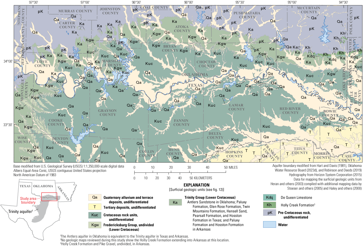
Surficial extent of the geologic units in the Antlers aquifer study area, southeastern Oklahoma, northeastern Texas, and southwestern Arkansas.
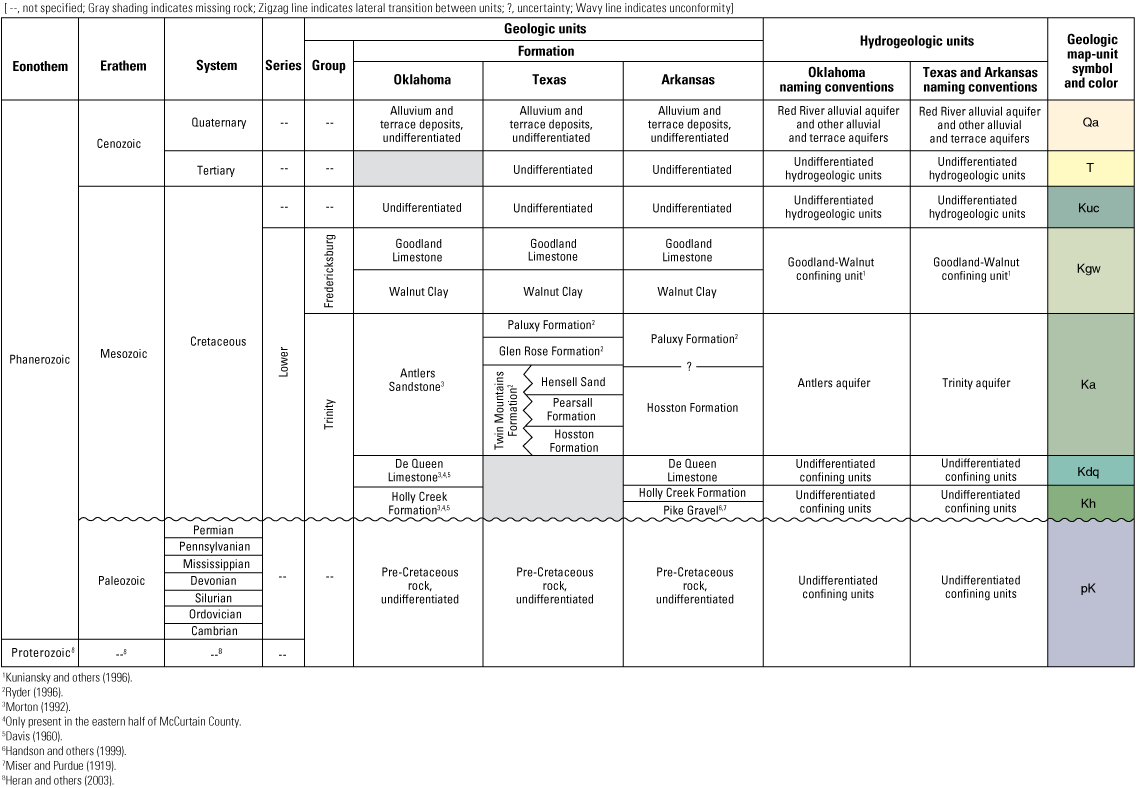
Surficial geologic and hydrogeologic units pertaining to the Antlers aquifer in southeastern Oklahoma.

Schematic hydrogeologic cross-section of the eastern part of the Antlers aquifer in McCurtain County, southeastern Oklahoma. Modified from Hartronft and others (1966).
The Antlers Sandstone was formed as a transgressive sheet of sand deposited along the shoreline of a slowly advancing sea (Davis, 1960; Frederickson and others, 1965; Huffman and others, 1975; Hart and Davis, 1981). The confined area of the Antlers aquifer is overlain by younger Cretaceous rocks (figs. 11–13; Hart and Davis, 1981; Morton, 1992). The upper part of the Antlers Sandstone is composed of sand, clay, weakly-cemented sandstone, sandy shale, and silt, with cross-bedded sandstone and lens-like bodies of conglomerate or calcium-carbonate-cemented sandstone also present throughout. The basal part of the Antlers Sandstone consists of conglomerate or calcareous-cemented sandstone with clay and silt (Hart and Davis, 1981; Morton, 1992). The Antlers Sandstone becomes progressively younger and thinner northward until it eventually pinches out from erosion at land surface.
The Trinity Group consists of multiple hydrogeologic units in Texas that include the Twin Mountains Formation, and, from oldest to youngest, its stratigraphic equivalents consisting of the Hosston Formation, Pearsall Formation, and Hensell Sand; at the top of the Trinity Group, the Twin Mountains Formation and Hensell Sand are overlain by the Glen Rose and Paluxy Formations (fig. 12; Robinson and Deeds, 2019). The Glen Rose Formation pinches out in northern Texas; according to Ashworth and Hopkins (1995, p. 20) “* * * where the Glen Rose thins or is missing, the Paluxy and Twin Mountains coalesce to form the Antlers Formation.” The Trinity Group extends to the east into Arkansas where it gradually thins and pinches out to the north and east (Ryder, 1996). In Arkansas, the Trinity Group consists of the Paluxy Formation of the Trinity Group, DeQueen Limestone of the Trinity Group, Holly Creek Formation of the Trinity Group, and Pike Gravel of the Trinity Group (Handson and others, 1999; Miser and Purdue, 1919).
Groundwater Quality
Data compiled from wells completed in the Antlers aquifer indicate groundwater quality varies throughout the study area. Groundwater-quality data were compiled from wells sampled by the OWRB and USGS (fig. 14). The OWRB sampled 30 wells completed in the unconfined part of the Antlers aquifer and 8 wells completed in the confined part in August of 2015 as part of their Groundwater Monitoring and Assessment Program (Groundwater Protection Council, 2015; OWRB, 2018). In addition, groundwater-quality data from nine wells sampled by the USGS between August 15, 1985, and September 11, 2020, were obtained from the USGS National Water Information System database (USGS, 2023); for the purposes of this analysis, data obtained from different wells collected by the OWRB and USGS were grouped into one dataset (fig. 14). The wells used for groundwater-quality analysis ranged in total depth from 20 to 651 ft below land surface with a mean total depth of 237 ft. This mean well depth is relatively shallow considering that the depth to the base of the Antlers aquifer exceeds 2,000 ft along the Red River, and as such, the groundwater-quality analysis is more representative of the shallow part of the aquifer than the deeper part of the aquifer.
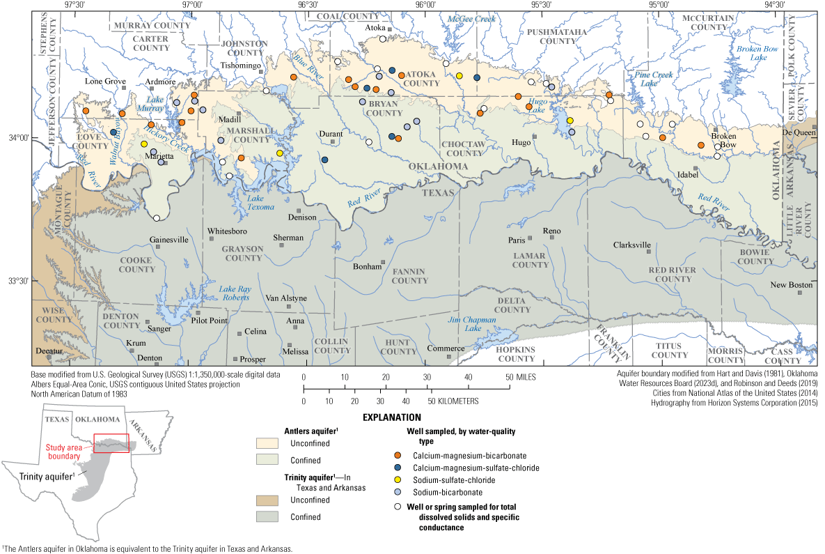
Groundwater wells from which groundwater-quality data were compiled for the Antlers aquifer, southeastern Oklahoma, 1985–2020.
TDS and specific conductance concentrations in the unconfined and confined parts of the Antlers aquifer were different. TDS concentrations measured in the groundwater samples compiled from the unconfined part of the Antlers aquifer ranged from 15 to 1,290 milligrams per liter (mg/L) with a mean concentration of 309 mg/L. TDS concentrations measured in groundwater samples compiled from the confined part of the Antlers aquifer ranged from 169 to 943 mg/L with a mean concentration of 557 mg/L. The mean TDS concentration for all groundwater samples compiled from wells completed in the Antlers aquifer was 383 mg/L. The U.S. Environmental Protection Agency (2017) established a secondary drinking-water standard of 500 mg/L for TDS concentrations. The State of Oklahoma, however, acknowledges a beneficial domestic use for general use (class II) groundwater with TDS concentrations of less than 3,000 mg/L and limited use (class III) groundwater with TDS concentrations of 3,000–5,000 mg/L (Groundwater Protection Council, 2015). All TDS concentrations were less than 3,000 mg/L in the groundwater samples compiled for the study. Specific conductance of groundwater samples from the unconfined part of the Antlers aquifer ranged from 27 to 2,010 microsiemens per centimeter at 25 degrees Celsius (µS/cm at 25 °C) with a mean value of 527 µS/cm. Specific conductance of groundwater samples from the confined part of the Antlers aquifer ranged from 252 to 1,690 µS/cm with a mean value of 914 µS/cm. The mean specific conductance for all groundwater samples collected from wells completed in the Antlers aquifer was 642 µS/cm.
Major cations and anions were examined using the Piper (1944) method (fig. 15). For the use of the Piper (1944) method, samples were required to include concentrations of selected major ions (calcium, magnesium, sodium, potassium, bicarbonate, carbonate, chloride, sulfate, and fluoride) in the groundwater-quality data. Major-ion concentrations were converted from milligrams per liter to milliequivalents per liter, and a cation-anion balance was done for each sample. Samples that did not contain all of the required major ions or had a difference in the cation-anion balance greater than 10 percent were excluded from further analysis. Only 43 of the 47 groundwater-quality samples met these criteria (figs. 14–15). Of those 43 groundwater-quality samples, 31 were collected from sites in the unconfined part of the Antlers aquifer, and 12 were collected from sites in the confined part of the Antlers aquifer (fig. 14). Data from the 43 samples were plotted on a Piper (1944) diagram for assessment of groundwater types and patterns for the unconfined and confined parts of the Antlers aquifer (fig. 15). The groundwater samples show a transition from the unconfined part of the Antlers aquifer, where groundwater generally has larger milliequivalent concentrations of calcium, magnesium, and bicarbonate (Ca, Mg, and HCO3, respectively) compared to the confined part of the aquifer in Oklahoma, which generally shows larger concentrations of sodium, potassium, and bicarbonate (Na, K, and HCO3, respectively). This correlates with analysis and conclusions made in the Hart and Davis (1981) report stating that TDS concentrations increase downdip, likely from dissolution of minerals over time. The calcium bicarbonate in the unconfined part of the Antlers aquifer indicates potential interaction between calcium carbonate cement and rainwater during recharge. The increase in concentrations of sodium, potassium, and bicarbonate in the confined part of the Antlers aquifer may be indicative of vertical leakage through the upper confining Goodland-Walnut confining unit into the Antlers aquifer (Morton, 1992).
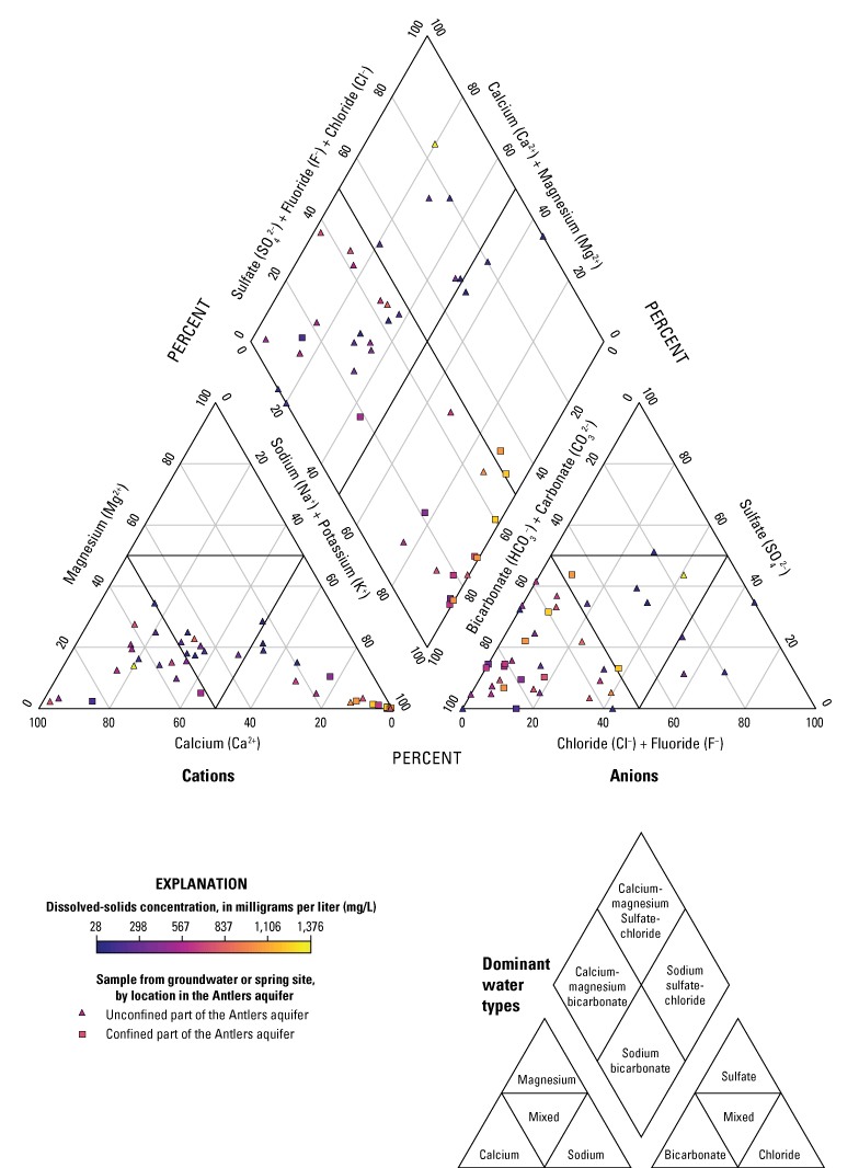
Relations between major cations and anions measured in groundwater-quality samples from wells completed in the Antlers aquifer, southeastern Oklahoma, 1985–2020.
Hydrogeologic Framework of the Antlers Aquifer
As part of this study, the hydrogeologic framework was updated for the Antlers aquifer. A hydrogeologic framework is a three-dimensional representation of an aquifer that describes the lithologic variability of the aquifer materials and how that aquifer interacts with surrounding geologic units at a scale that captures regional controls on groundwater flow (Smith and others, 2021). The hydrogeologic framework for the Antlers aquifer includes updated (from previous publications such as Morton [1992]) definitions of the aquifer extent and potentiometric surface that were provided by OWRB (2023e), as well as a description of the hydraulic and textural properties of aquifer materials.
Aquifer Extent and Thickness
The geographic extent of the Antlers aquifer (fig. 1) was updated by the OWRB. The previous Antlers aquifer extent (OWRB, 2023e) was delineated when the initial MAY was established in 1995. In updating the Antlers aquifer extent, the OWRB used a combination of mapped geologic contacts, professional interpretation of covered geologic contacts, and consideration of existing dedicated land areas for some Antlers aquifer groundwater permit holders at or near the aquifer boundary.
The Oklahoma Geological Survey has updated many of the geologic maps for Oklahoma by incorporating information from multiple geologic quadrangles published since the first determination of MAY in 1995. Most of the western half of the Antlers aquifer extent is covered by two Oklahoma Geological Survey geologic quadrangles (Stanley and Chang, 2012; Chang and Stanley, 2013), which mapped geologic units in more detail than was available in 1995. The eastern half of the Antlers aquifer extent has no new geologic mapping beyond what was available in 1995. The OWRB identified areas where the OWRB (2023e) mapped extent of the Antlers aquifer did not align with the mapped extent of the Antlers Sandstone in Stanley and Chang (2012) and Chang and Stanley (2013), as well as areas where the Antlers Sandstone was not depicted but where other lines of evidence indicated that the Antlers aquifer was likely present.
At the western edge of the Antlers aquifer extent in Love and Carter Counties, the aquifer extent was updated to match the mapped surficial contact between the Antlers Sandstone and older pre-Cretaceous rocks (Chang and Stanley, 2013; Stanley and Chang, 2012). A small area in the southern part of the outcrop area was covered by alluvium of the Red River, and the Antlers aquifer extent was estimated to continue in subcrop to the Oklahoma-Texas border (fig. 11). The southern edge of the Antlers aquifer follows the Oklahoma-Texas border, where the hydrogeologic units of the aquifer are presumed to be buried by younger hydrogeologic units. The northern extent of the Antlers aquifer followed the mapped contact between the Antlers Sandstone and older pre-Cretaceous rocks, except where the Antlers Sandstone crossed the mapped alluvium of Walnut Bayou and the Washita River where the contact was interpolated. Several previously mapped isolated outcrops of Antlers Sandstone were not included in the OWRB’s updated extent. A previously mapped outcrop of the Antlers Sandstone north of the Washita River was excluded from the updated aquifer extent after examination based on the location and altitude of geologic units that crop out to the south of the Washita River. The Washita River was determined to have completely eroded through the Antlers Sandstone, hydrologically separating the Antlers Sandstone to the north from the main body of the formation south of the Washita River. Parts of the previously mapped Antlers aquifer extent in Pushmataha and Choctaw Counties also were removed because older units were found to crop out that are not considered part of the Antlers aquifer. Because detailed geologic quadrangles were not available for the eastern part of the Antlers aquifer extent, coarse-scale geologic maps (Marcher and Bergman, 1983) were used to define the aquifer extent in this area. The aquifer extent was interpolated and estimated as necessary where data were lacking, such as below surficial alluvial features. Some areas with existing Antlers aquifer groundwater-use permits and dedicated lands were left in the aquifer extent to avoid splitting the existing dedicated lands.
The updated extent of the Antlers aquifer encompasses approximately 2,746,648 acres (fig. 1; table 6) in Oklahoma and extends from near Marietta, Okla., in the west to Arkansas to the east and from near Atoka, Okla., in the north, to Texas in the south. The unconfined part of the aquifer covers approximately 1,117,835 acres in Oklahoma (fig. 1; table 6).
Table 6.
Conceptual-model water budget of estimated mean annual inflows and outflows for hydrologic boundaries for the Antlers aquifer, southeastern Oklahoma, 1980–2022.[All units in acre-feet per year unless otherwise stated. in/yr, inch per year; SWB, Soil-Water Balance; USGS, U.S. Geological Survey; OWRB, Oklahoma Water Resources Board; NWI, National Wetlands Inventory; --, not quantified; %, percent]
| Hydrologic boundary | Unconfined part of the Antlers aquifer1 | Confined part of the Antlers aquifer2 | Antlers aquifer total in the study area3 | Percentage of water budget | Confidence of accuracy of component estimates | Notes |
|---|---|---|---|---|---|---|
| Recharge4 | 799,252 | 0 | 799,252 | 100% | High | 8.58 in/yr or 19% of mean annual precipitation estimated using SWB code. |
| Vertical leakage | -- | -- | -- | -- | Low | Assumed to be a negligible part of water budget. |
| Net change in groundwater storage | -- | -- | -- | -- | Low | Assumed to be a negligible part of water budget. |
| Total inflow | -- | -- | 799,252 | 100% | -- | |
| Net streambed seepage4 | 660,253 | 0 | 660,253 | 82.6% | Medium | Estimated from base-flow data at selected USGS streamgages. |
| Net lateral groundwater flow | -- | 128,355 | 128,355 | 16.1% | Low | Unknown; calculated as balance of water budget. |
| Saturated-zone evapotranspiration4 | 7,161 | 0 | 7,161 | 0.9% | Low | 2.00 in/yr multiplied by estimating the total NWI wetland area of 42,965 acres (U.S. Fish and Wildlife Service, 2014) overlying the unconfined part of the Antlers aquifer. Evapotranspiration rate adjusted from White (1932) based on the difference in climate, and longer growing season from that study. |
| Well withdrawals | -- | -- | 3,483 | 0.4% | Medium | From OWRB reported water-use data (table 3). Mean reported groundwater use for the period 1980–2022 (OWRB; 2023b). |
| Total outflow | -- | -- | 799,252 | 100% | -- |
Aquifer Depths
In the unconfined part of the Antlers aquifer, the top of the aquifer was defined as the land-surface altitude obtained from a 10-m (horizontal resolution) digital elevation model (DEM; USGS, 2015). The altitudes of the top of the aquifer in the confined part and the base of the aquifer in the unconfined and confined parts of the Antlers aquifer were digitized and interpolated from contour maps by Morton (1992) and Hart and Davis (1981), which were derived from interpretation and correlation of 230 geophysical logs from oil and gas wells.
The top of the Antlers aquifer dips south-southwest at a rate of 35–90 feet per mile (ft/mi), with a mean dip of approximately 60 ft/mi (Morton, 1992). The depth of the top of the Antlers aquifer exceeds 1,500 ft in the far southeastern corner of McCurtain County, Okla. The base of the Antlers aquifer also dips south-southeast at a steeper rate of 35–105 ft/mi with a mean dip of approximately 75 ft/mi (Morton, 1992). The base of the aquifer dips greater to the southeast than does the top, resulting in a thickening of the aquifer to the south-southeast. The deepest depth to the base of the Antlers aquifer from land surface is greater than 2,500 ft. The thickness of the Antlers aquifer varies greatly from north to south (Hart and Davis, 1981). The Antlers aquifer saturated thickness ranges from 0 ft in the northernmost unconfined part—increasing to the southeast to almost 1,200 ft in southeastern Oklahoma—to more than 2,000 ft south of the Red River (Morton, 1992).
Aquifer Base
For the purposes of this report, the base of the Antlers aquifer is considered to be the base of fresh groundwater (OWRB, 2023c). Data from Robinson and Deeds (2019) that were collected as part of the Texas Water Development Board’s (TWDB) Brackish Resources Aquifer Characterization System, were used to determine the base of fresh groundwater for the Antlers aquifer.
Robinson and Deeds (2019) spatially estimated the depths of TDS concentrations in the five geologic units (Hosston Formation, Pearsall Formation, Hensell Sand, Glen Rose Formation, and Paluxy Formation; fig. 12) in the northern part of the Trinity aquifer at 1,000, 3,000, and 10,000 mg/L for each of the geologic units using a combination of groundwater samples and interpretation of geophysical logs from wells completed in the Trinity aquifer. The altitude of the top surface of each geologic unit was correlated to the 1,000-, 3,000-, and 10,000-mg/L TDS contours for the respective surface. For the purposes of this report and to align with water-quality limits set by the State of Oklahoma, a 5,000-mg/L TDS contour (fig. 16A) was interpolated as the boundary between fresh and saline groundwater for each of the geologic units by using the 3,000- and 10,000-mg/L TDS extents determined by Robinson and Deeds (2019). Altitude values were assigned to points along the 5,000-mg/L contour lines that corresponded to the altitude of the top of each geologic unit (Robinson and Deeds, 2019). An altitude surface was interpolated between the 5,000-mg/L line of the lowermost geologic unit (Hosston Formation) and the uppermost geologic unit (Paluxy Formation). The altitude surface created from this interpolation was merged with altitude surfaces for the top and base of the Antlers aquifer from Morton (1992) as well as the land surface altitude (for the unconfined part). This resulted in a three-dimensional boundary of altitudes for the base of usable groundwater (freshwater zone) for the Antlers aquifer (fig. 16). Beyond where the 5,000-mg/L TDS altitude surface intersected the altitude of the top of the Antlers aquifer, groundwater was considered to have TDS concentrations that exceeded 5,000 mg/L (saline zone) and was therefore considered to be unusable as freshwater for the purposes of the State of Oklahoma (OWRB, 2023c).


A, Map showing estimated altitude of the base of fresh groundwater and areas with saline water that exceed 5,000 milligrams per liter (mg/L) total dissolved solids (TDS) concentration in the Antlers aquifer, southeastern Oklahoma, northeastern Texas, and southwestern Arkansas, with B, inset map and associated schematic cross-section showing the fresh-saline water boundary at 5,000-mg/L TDS concentration along line of section A–A′ in the Antlers aquifer, southeastern Oklahoma and northeastern Texas
Potentiometric Surface and Saturated Thickness
Potentiometric-surface maps illustrate the altitude at which the water would have risen to in tightly cased wells at a specified time (Fetter, 2001); the potentiometric surface is usually contoured or spatially interpolated from synoptic water-table altitude measurements in many wells across the extent of an aquifer. Potentiometric-surface maps are used to indicate the general directions of groundwater flow in an aquifer. Groundwater generally flows perpendicular to potentiometric contours in the direction of decreasing contour altitude (Freeze and Cherry, 1979). An aquifer with substantial vertical flow can have multiple potentiometric surfaces because potentiometric heads in the aquifer change with depth because of the presence of clay or other local confining units within the aquifer. The wells used for synoptic water-level measurements in the Antlers aquifer were completed at depths that ranged from 25 to 730 ft below land surface with a mean depth of 233 ft below land surface, which is relatively shallow for the aquifer. The potentiometric surface described in this report approximates the uppermost part of the Antlers aquifer, commonly referred to as the water table (Alley and others, 1999).
Hart and Davis (1981) and Morton (1992) published some of the earliest potentiometric-surface maps for the Antlers aquifer. Hart and Davis (1981) measured groundwater levels in 1975 and 1976 to observe how they varied over time and found that they generally changed by less than 1 ft over the observation period. Morton (1992) used data from synoptic measurements collected in 1970 to construct a potentiometric-surface map, simulate aquifer conditions, and create predictive potentiometric surface-maps for 1990, 2000, 2010, 2020, 2030, and 2040.
The potentiometric surface for the Antlers aquifer in winter 2022 was mapped primarily by using 68 groundwater-level measurements (depth to water, in feet below land surface) collected in Oklahoma by the OWRB between February 28, 2022, and March 9, 2022. Wells used for synoptic measurements were mostly domestic and irrigation wells that were unused (not pumping or recently pumped) at the time of measurement. Two of the groundwater-level measurements were not included in the map and analyses because either the well was being pumped at the time of measurement or the well was determined to be completed in a different aquifer. For northeastern Texas, where no measurements were collected by the OWRB, 13 groundwater-level measurements made between November 16, 2021, and December 1, 2022, that were contemporaneous with the OWRB measurements were obtained from the TWDB Groundwater Database (TWDB, 2023). The TWDB groundwater-level measurements were used to provide data for the part of the study area in Texas because OWRB only measured groundwater levels in wells in Oklahoma. Where applicable, TWDB data from wells with multiple or historical measurements were checked to ensure that there were not large fluctuations in groundwater levels and the measurements used were representative of groundwater levels during the synoptic measurement completed in Oklahoma.
At each well location, every groundwater-level measurement was subtracted from the land-surface altitude, derived from a 10-m DEM (USGS, 2015), to determine the groundwater-level altitude in feet above the North American Vertical Datum of 1988 (NAVD 88). Groundwater-level altitude data were then used to create a potentiometric-surface map for 2022 (fig. 17). For areas with little or no groundwater-level altitude data (mostly the aquifer extent in Texas), contours from the observed potentiometric-surface map for 1970 published by Morton (1992) were used to add control points to help shape contour lines in those areas. The 2022 potentiometric surface was shallow along the western and northwestern parts of the Antlers aquifer and deeper in the southeastern parts of the aquifer. Local flow in the Antlers aquifer is generally from north to south, following the dip of the aquifer (fig. 17). The general patterns and directions of groundwater flow were similar between all three of the potentiometric maps: 1970 (Morton, 1992), 1975 (Hart and Davis, 1981), and 2022 (fig. 17). The general shapes of the potentiometric-surfaces, along with the resulting flow directions, were also similar between the 2022 potentiometric-surface map and the simulated potentiometric surface created by Morton (1992) for the year 2020. The similarities between previously created potentiometric-surface maps and the 2022 potentiometric-surface map indicate that groundwater levels and storage volumes in the Antlers aquifer have remained relatively stable over the past 50 years.

Potentiometric-surface contours and general direction of groundwater flow in the Antlers aquifer, southeastern Oklahoma, northeastern Texas, and southwestern Arkansas, November 2021–December 2022.
The saturated thickness of fresh groundwater in the Antlers aquifer was determined by subtracting the altitude of the base of the aquifer from the altitude of the top of the aquifer (for the confined part) or the altitude of the potentiometric surface (for the unconfined part). The potentiometric saturated thickness of fresh groundwater in the Antlers aquifer was determined by subtracting the altitude of the base of the aquifer from the altitude of the 2022 potentiometric surface. The potentiometric saturated thickness of the Antlers aquifer increases from 0 ft in the northern part of the Antlers aquifer to more than 1,000 ft in the southeastern parts of the Antlers aquifer and over 1,500 ft in northeastern Texas (fig. 18). The mean aquifer saturated thickness for the Antlers aquifer is about 434 ft.

Estimated potentiometric saturated thickness of fresh groundwater in the Antlers aquifer, southeastern Oklahoma, northeastern Texas, and southwestern Arkansas, November 2021–December 2022.
Hydraulic and Textural Properties
The distribution and variability of hydraulic and textural properties of aquifer materials, especially the horizontal hydraulic conductivity, were assumed to be the primary controls on groundwater flow in the Antlers aquifer. Multiple methods were used to estimate the range and central tendency of horizontal hydraulic conductivity values in the aquifer. These methods included a multiple-well aquifer test, slug tests, and analysis of lithologic descriptions from wells completed in the Antlers aquifer. The unconfined part the Antlers aquifer is approximately 80 percent sand; the percentage of sand decreases to less than 40 percent as the aquifer thickens to the south (Hart and Davis, 1981).
Hydraulic Properties Estimated From a Multiple-Well Aquifer Test
A multiple-well aquifer test involving preexisting wells GW-04, GW-07, and GW-08 (fig. 1) was completed as part of this investigation in November 2022 in the eastern part of the Antlers aquifer to determine transmissivity, hydraulic conductivity, and storage coefficient values for the aquifer. Aquifer transmissivity is a measure of the amount of water that can be transmitted horizontally through a unit width by the full saturated thickness of the aquifer (Fetter, 2001). Hydraulic conductivity is a measure of the capacity of a porous medium to transmit water (Driscoll, 1986). The storage coefficient of an aquifer is the volume of water that a permeable unit will absorb or expel from storage per unit surface area per change in head (Fetter, 2001). Data from this aquifer test are included in the accompanying data release (Fetkovich and others, 2025).
The multiple-well aquifer test involved withdrawing groundwater from well GW-07 (hereinafter referred to as the “pumping well”) at a constant rate of approximately 160 gallons per minute for approximately 48 hours until groundwater levels in nearby observation wells GW-04 and GW-08 stabilized (figs. 1, 19). The withdrawal of groundwater induced a maximum drawdown of 32.87 ft in the pumping well, 2.38 ft in well GW-04 (approximately 978 ft from the pumping well), and 1.20 ft in well GW-08 (approximately 1,530 ft from the pumping well) after approximately 45 hours. After the pump was turned off, groundwater levels continued to be monitored to observe the recovery in each well until groundwater levels returned to their pretest static levels observed prior to the approximately 48-hour period of groundwater withdrawals. Groundwater levels in wells GW-04 and GW-07 recovered to 100 percent and 98 percent, respectively, of their pretest levels. Data collection from well GW-08 was stopped prematurely, which resulted in a recovery of only 46 percent of the original groundwater level in that well. Maximum recovery of groundwater levels was achieved after about 7.5 days post-pumping, as observed in wells GW-04 and GW-07. Water-level observations varied between the three wells used for this aquifer test, so each well was analyzed independently using both the drawdown and recovery data, where data were sufficient. Owing to the recorder being removed prematurely in GW-08 resulting in insufficient recovery, recovery data at this well were not viable for analysis. The pumping well (GW-07) was not constructed in a way that allowed for installation of a recorder, and although water-level data were collected intermittently from this well during the test by using a manual water-level tape, these data were not sufficient for analysis. Data that were analyzed included the drawdown and recovery data from well GW-04 and the drawdown data from well GW-08. The aquifer test data were analyzed using the AQTESOLV software package (fig. 19A–C; Hydrosolve, Inc., 2011). The depths of the test and observation wells with casing information were input to the AQTESOLV program to correct for partial penetration of the aquifer. Groundwater levels from the pumping and recovery periods were matched to the Hantush (1960) method, which accounts for partially penetrating wells and estimates anisotropy in a leaky confined aquifer (fig. 19A–C). The test-well location and analytical-model solution indicated a leaky-confined aquifer (Lohman, 1972). One analysis was performed for each well by using the drawdown and recovery observations and the Hantush (1960) method in either standard time or Agarwal equivalent time (Duffield, 2025). Agarwal equivalent time is an adjustment of the time to an equivalent time that only includes time of recovery (Duffield, 2025). The values from each of the analyzed datasets were compiled into ranges for transmissivity, hydraulic conductivity, and the storage coefficient.

A, Pumping drawdown data curve for well GW-04, B, pumping recovery curve for well GW-04, and C, pumping drawdown curve for well GW-08, with best-fit Hantush (1960) method for leaky confined aquifer analysis results (Fetkovich and others, 2025).
Transmissivities determined by using the Hantush (1960) method ranged from 3,598 to 5,647 square feet per day (ft2/d). Using the screened interval of 61 ft for the test well, the hydraulic conductivities ranged from 6.79 to 10.65 feet per day (ft/d). The storage coefficient from the Hantush (1960) method ranged from 0.00056 to 0.00080. The transmissivity, hydraulic conductivity, and storage coefficient derived from the multiple-well aquifer test are likely to be more accurate than hydraulic values derived using other methods, such as from grain size or laboratory tests of aquifer material, because flow is induced across a larger volume of the aquifer during the aquifer test than during other tests (Lohman, 1972). However, these hydraulic property values represent local conditions and are not necessarily indicative of the mean or range of regional hydraulic property values.
Hydraulic Properties Estimated From Slug Tests
Multiple slug tests were performed at four wells (GW-03, GW-04, GW-05, and GW-09; fig. 1) to assess repeatability and well integrity. One selected well that was not included in this report did not appear to be hydraulically connected with the aquifer and was not included in the analyses. Both mechanical and poured slugs were utilized depending on the construction of each well.
For each poured slug test, a volume of water, either 5, 10, or 15 gallons was rapidly poured into the well casing. Water-level changes were recorded with an electronic recording pressure transducer set at a 0.25-second measurement frequency. The near instantaneous rise and subsequent fall of the water level in response to the poured slugs were recorded and analyzed as a falling head test using the Bouwer and Rice method, as described by Halford and Kuniansky (2002).
In a mechanical slug test, the existing groundwater in the well is displaced instead of adding a “slug” of actual water to the well. The groundwater is displaced by rapidly lowering a 4-ft-long section of polyvinyl chloride (PVC) pipe filled with sand and capped on each end below the groundwater level in the well; the section of PVC pipe is then rapidly raised above the groundwater level in the well. The change in groundwater level and time for the well to return to the original pretest groundwater level is recorded. The test is performed multiple times. Each time, the change in water level and time for the well to return to the original groundwater level are recorded. The slug test responses (changes in groundwater levels) were analyzed by using the AQTESOLV software package (Hydrosolve, Inc, 2011) and were matched to an analytical solution dependent on the construction of the well and the observed response of each test.
Methods explained in Butler (1998) were used in combination with well construction information, where available, to aid in determining the most appropriate analytical solution for each well used in the slug tests. Selected wells were completed in either the unconfined or confined part of the Antlers aquifer (fig. 1). Analytical solutions used in the analysis of the slug tests included the Hvorslev (1951) solution for wells completed in the confined part of the aquifer and the Bouwer and Rice (1976) and Kansas Geological Survey (Hyder and others, 1994) solutions for wells completed in the unconfined part of the aquifer. One analytical solution was selected for each well, depending on available well construction information and following guidelines from Butler (1998). Further details for the analyses of the slug tests are included in the accompanying data release (Fetkovich and others, 2025).
Transmissivities determined from the analytical solutions ranged from 399 to 6,416 ft2/d. Hydraulic conductivity values determined from the analytical solutions ranged from 0.84 to 12.15 ft/d. The storage coefficient of an aquifer is equal to the specific storage multiplied by the saturated thickness (Fetter, 2001). The storage coefficient determined from the analytical solutions for the confined part of the aquifer was 0.004. The storage coefficient of the confined part of the aquifer was determined from analysis of GW-09, which was the only slug test performed in a confined well. Because specific storage is generally very small, the storage coefficient in unconfined aquifers is generally considered to be equivalent to specific yield (Driscoll, 1986). Specific storage was estimated to range from 1.1 × 10⁻⁶ to 5.0 × 10⁻⁵ foot−1 using a combination of values estimated from slug test analyses and values taken from Batu (1998). Because the storage coefficient is dependent upon specific yield, a specific yield value of 0.10 was used, estimated for the Trinity aquifer by Jigmond and others (2014). Using this specific yield value in slug test analyses from unconfined wells resulted in storage coefficient values that ranged from 0.10 to 0.11. These hydraulic values represent local conditions and are not necessarily indicative of the hydraulic property values of larger areas (regions).
Horizontal Hydraulic Conductivity Estimated From Lithologic Logs
Horizontal hydraulic conductivity distribution across the Antlers aquifer was estimated by using information obtained from lithologic logs (OWRB, 2023d) that were reported to the OWRB by drillers. Reported lithologic logs were filtered to include only sections of logs that were located between the top and base of the Antlers aquifer. Textural descriptions and terms provided in the lithologic logs were categorized and converted to percent-coarse-material values by using methods described in Mashburn and others (2014). Textural descriptions and terms varied between drillers. To simplify and standardize the lithologic logs, lithologic descriptions from wells completed within the Antlers aquifer and the lithologic descriptions for the surrounding geologic units were reclassified into 12 categories that were each assumed to include a specific percentage of coarse material based on known grain sizes of materials listed in the lithologic logs. This reclassification is similar to a modified version of the methods described in Mashburn and others (2014) in which granite (lower confining unit of the Antlers aquifer), shale, clay, silt, very fine sand, dolomite, limestone, fine sand, coal, medium sand, coarse sand, and gravel each contain 0, 10, 10, 10, 20, 30, 30, 30, 40, 50, 70, and 90 percent-coarse material, respectively. The respective percent-coarse-material value was then assigned to each lithologic depth interval. Lithologic depth intervals assigned as granite were removed, as granite is not considered part of the Antlers aquifer. The percent-coarse-material value for each lithologic log was computed as the thickness-weighted mean of percent-coarse-material values assigned to the lithologic categories found within the log. The theoretical maximum percent-coarse-material value for any lithologic log was 90 percent (all gravel), and the theoretical minimum percent-coarse-material value for any lithologic log was 10 percent (all clay, shale, or silt). A total of 1,520 usable lithologic logs (OWRB, 2023d) were included in the percent-coarse-material analysis. Logs with obvious errors were corrected to extract as much useful information as possible, whereas logs with inscrutable errors were discarded.
The horizontal hydraulic conductivity estimated from lithologic logs ranged from 0.87 to 10.65 ft/d, using the maximum and minimum estimated horizontal hydraulic conductivity between the aquifer test, slug tests, and previously published values (Hart and Davis, 1981). Hart and Davis (1981) reported a horizontal hydraulic conductivity range of 0.87–3.75 ft/d. Although the slug test analyses determined a maximum horizontal hydraulic conductivity of 12.15 ft/d, this value was determined from a slug test on the same well that was used for the multiple-well aquifer test, which resulted in a value of 10.65 ft/d. Multiple-well aquifer tests are considered to be more accurate than slug tests because the former are affected by a wider area extending beyond the influence of a slug test; therefore, the horizontal hydraulic conductivity range of 0.87–10.65 ft/d was used. Using this range and methods from Ellis and others (2017), the following equation was developed by correlating the minimum and maximum horizontal hydraulic conductivity values to 10 and 90 percent-coarse material, respectively, and performing a linear regression to characterize the relation between horizontal hydraulic conductivity and the percentage-coarse material value for the Antlers aquifer:
whereKh
is the horizontal hydraulic conductivity, in feet per day; and
Ps
is the percent-coarse-material value.
Equation 1 is used in this report to estimate horizontal hydraulic conductivity values for lithologic logs from wells completed in the Antlers aquifer. The lithologic-log estimated horizontal hydraulic conductivity values ranged from 0.87 to 9.02 ft/d with a mean of 3.31 ft/d (fig. 20).
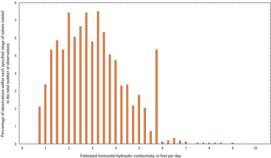
Distribution of estimated horizontal hydraulic conductivity values estimated from lithologic logs (Oklahoma Water Resources Board [OWRB], 2023d) obtained for wells completed in the Antlers aquifer, southeastern Oklahoma.
Aquifer Storage Properties and Estimated Groundwater Storage
Total groundwater storage, in acre-feet, for the Antlers aquifer was estimated by the following formula, modified from Fetter (2001):
whereSy
is specific yield, dimensionless;
Ss
is specific storage, in feet-1;
STp
is the mean potentiometric saturated thickness, measured from the base of the aquifer to the potentiometric surface, in feet;
STa
is the mean saturated thickness, measured from the base of the aquifer to the top of the aquifer, in feet; and
A
is the aquifer area, in acres.
For this report, the value for specific yield (Sy) was set to 0.1 in accordance with Jigmond and others (2014). The value for specific storage (Ss) was estimated to be in the range of 1.1 × 10⁻⁶ to 5 × 10⁻⁵ foot−1 based on values from slug tests and ranges in Batu (1998). The base of the Antlers aquifer and the 2022 potentiometric surface were used to create surface rasters for each set of data. The value for the mean potentiometric saturated thickness (STp) was determined by subtracting the altitude surface raster of the base of the Antlers aquifer from the 2022 potentiometric altitude surface raster and calculating the mean value for the aquifer in Oklahoma. The value for the mean saturated thickness (STa) was determined by subtracting the altitude of the base of the Antlers aquifer from either the altitude of the 2022 potentiometric surface or the altitude of the top of the aquifer (Morton, 1992) and calculating the mean for the aquifer in Oklahoma. Using the values for Sy and Ss along with the values of 434 ft for the mean saturated thickness (STa) and 621 ft for the mean potentiometric saturated thickness (STp) in equation 1 with the aquifer area (2,746,648 acres), the total groundwater storage for the Antlers aquifer is estimated to range from about 120,000,000 to 156,000,000 acre-ft.
Conceptual Groundwater Flow Model and Water Budget
Two key components for simulating a groundwater-flow system are the conceptual groundwater flow model (hereinafter referred to as the “conceptual model”) and the resulting water budget. A conceptual groundwater-flow model is a simplified representation of the groundwater-flow system that accounts for the major inflows and outflows across hydrologic boundaries within a water budget. This conceptual model is thus the means for approximating the water budget for an aquifer. Hydrologic boundaries are boundaries based on the hydrogeologic framework, hydrologic controls, and climatic conditions where water flows into or out of the aquifer, thus potentially changing the total storage of the aquifer. The conceptual model for the Antlers aquifer provided a water budget (fig. 21; table 6) that was used to quantify net groundwater flows across each identified hydrologic boundary for the Antlers aquifer for the 1980–2022 study period.
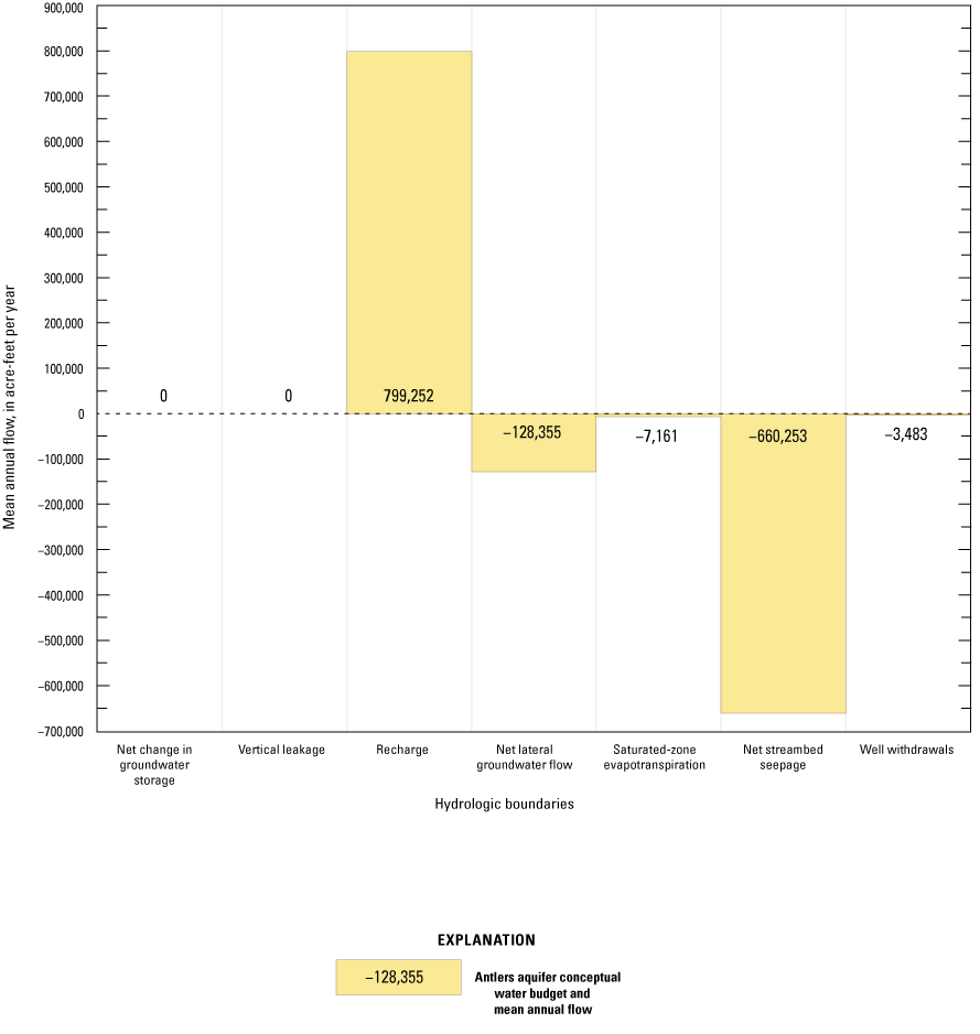
Estimated mean annual inflows and outflows by hydrologic boundary for the conceptual groundwater-flow model and water budget of the Antlers aquifer, southeastern Oklahoma, 1980–2022.
Hydrologic Boundaries
Hydrologic boundaries in a conceptual model represent actual sources (inflows) and sinks (outflows) of water to and from an aquifer. In this report, water crossing a hydrologic boundary is referred to as “net inflow” or “net outflow,” depending on which flow component dominates.
Recharge
For this report, recharge is defined as the amount of precipitation that infiltrates at the land surface and reaches the saturated zone of the aquifer. Areal recharge from precipitation is the predominant inflow to the Antlers aquifer. Factors such as precipitation rates, evapotranspiration rates, soil and sediment permeability, vegetation cover types, and the gradient of the land surface affect rates of recharge (Rogers and others, 2023). Recharge rates are difficult to quantify because of spatial and temporal variability; however, recharge rates can be estimated from other measurements and climatological data. Two methods were used to estimate recharge rates for this report: (1) the Soil-Water-Balance (SWB) code (Westenbroek and others, 2010) was used to estimate spatially distributed recharge rates for the 1980–2022 study period; and (2) the water-table-fluctuation (WTF) method (Healy and Cook, 2002) was used to estimate localized recharge rates during 2013–22.
Soil-Water-Balance Code
For the 1980–2022 study period, the amount and spatial distribution of daily groundwater recharge was used to estimate the mean annual recharge to the Antlers aquifer for the study period. Recharge was estimated by using the SWB code (SWB version 1; Westenbroek and others, 2010). The SWB code uses a modified Thornthwaite-Mather (Thornthwaite and Mather, 1957) SWB method on a gridded data structure to compute the daily amount of infiltration, accounting for losses, that exceeds the storage capacity of the plant root zone. Input data required to estimate recharge using the SWB code include precipitation, air temperature, soil-water storage capacity, hydrologic soil group, surface-water flow direction, and land-cover type (Westenbroek and others, 2010). The input data files and output recharge data files were included in the data release (Fetkovich and others, 2025) that accompanies this report. The Soil-Water-Balance code uses the following equation (modified from Westenbroek and others, 2010):
whereR
is recharge, in inches per day;
P
is precipitation, in inches per day;
S
is snowmelt, in inches per day;
Ri
is surface runoff, in inches per day;
Int
is plant interception, in inches per day;
R0
is surface runoff outflow, in inches per day;
Pet
is potential evapotranspiration, in inches per day; and
ΔSm
is the change in soil moisture, in inches per day.
Input data needed for the SWB code were assigned to a user-specified grid that consisted of 917 columns by 372 rows of cells that were each 1,000 ft by 1,000 ft. Climate data inputs (daily precipitation, minimum temperature, and maximum temperature grids for 1980–2022) were obtained from the Daymet database (version 4; Thornton and others, 2020). Soil properties (soil-water storage capacity and hydrologic soil group) were obtained from the Gridded Soil Survey Geographic database (USDA, 2021). Land-cover types were obtained from the National Land Cover Database (fig. 2; Multi-Resolution Land Characteristics Consortium, 2023) and resampled to the SWB grid resolution by using the most common land-cover type as a percentage of the total coverage within each cell. Flow direction was derived by calculating the land-surface gradient by using the D8 method (Greenlee, 1987) from a 10-m DEM (USGS, 2015); any depressions were filled by using the ArcGIS Fill tool (Esri, 2023) after the DEM was resampled to the SWB grid. Filling depressions in the DEM ensures correct routing of surface runoff and eliminates isolated areas that could result in unrealistically high amounts of recharge.
Potential evapotranspiration was calculated by using the Hargreaves and Samani (1985) method for a reference latitude range of 34.5–35.4 degrees. Land-cover types (fig. 2; Multi-Resolution Land Characteristics Consortium, 2023) were used in conjunction with hydrologic soil groups to partition daily precipitation into plant interception (Int) and surface runoff (Ri and R0) components and assign plant root-zone depths. The root-zone depths for grass/pasture and forest/shrubland (the dominant land-cover types for land overlying the aquifer; fig. 2) varied with soil texture but ranged from about 0.7 to 1.5 ft after being scaled to 40 percent of the values used by Westenbroek and others (2010), which were in permeable glacial deposits in Wisconsin. The root-zone depths were scaled by 40 percent to account for the difference in root zones between the study area and Wisconsin, where Westenbroek and others (2010) estimated the initial root zone depths. The maximum volume of water available in the root zone is calculated by multiplying the soil-water storage capacity by the root-zone depth. Changes in soil moisture (ΔSm) exceeding the soil-water storage capacity were assumed to be recharge (R) to the saturated zone. Smaller root-zone depths resulted in increased recharge and decreased evapotranspiration of water from the root zone, and larger root-zone depths resulted in decreased recharge and increased evapotranspiration of water from the root zone. Recharge from irrigation was not simulated by SWB but was assumed to be negligible given the relatively small amount of irrigation groundwater use in the study area.
Recharge was assumed to only occur in the unconfined part of the Antlers aquifer; therefore, the output data from the SWB model were summarized within the unconfined part of the Antlers aquifer. Recharge over large lakes was considered to be zero because open bodies of water do not contribute to recharge in the SWB calculation. The spatially distributed mean annual SWB-estimated recharge rate (SWBR) for the 1980–2022 study period was 8.58 in/yr, or about 19 percent of the mean annual precipitation of 45.2 in/yr. The annual SWBR ranged from 3.3 in. for 2005 to 18.8 in. for 2015, which respectively were years of much lower and higher precipitation compared to the mean annual precipitation (figs. 4, 22A). The ratio of mean monthly recharge to mean monthly precipitation is the recharge efficiency. During the study period, recharge efficiency was greatest during November–March when evapotranspiration is generally at a minimum; recharge during these months exceeded 20 percent of precipitation (fig. 22B). Recharge efficiency was lowest in July and August when evapotranspiration is generally at a maximum; recharge during these months was less than 9 percent of precipitation (fig. 22B). Spatially, SWBR increases from west to east across the unconfined part of the aquifer (fig. 23), which follows the general increase in precipitation from west to east (Thornton and others, 2020; Oklahoma Mesonet, 2023), with the highest SWBR rates generally being in the eastern half of the aquifer (fig. 23).
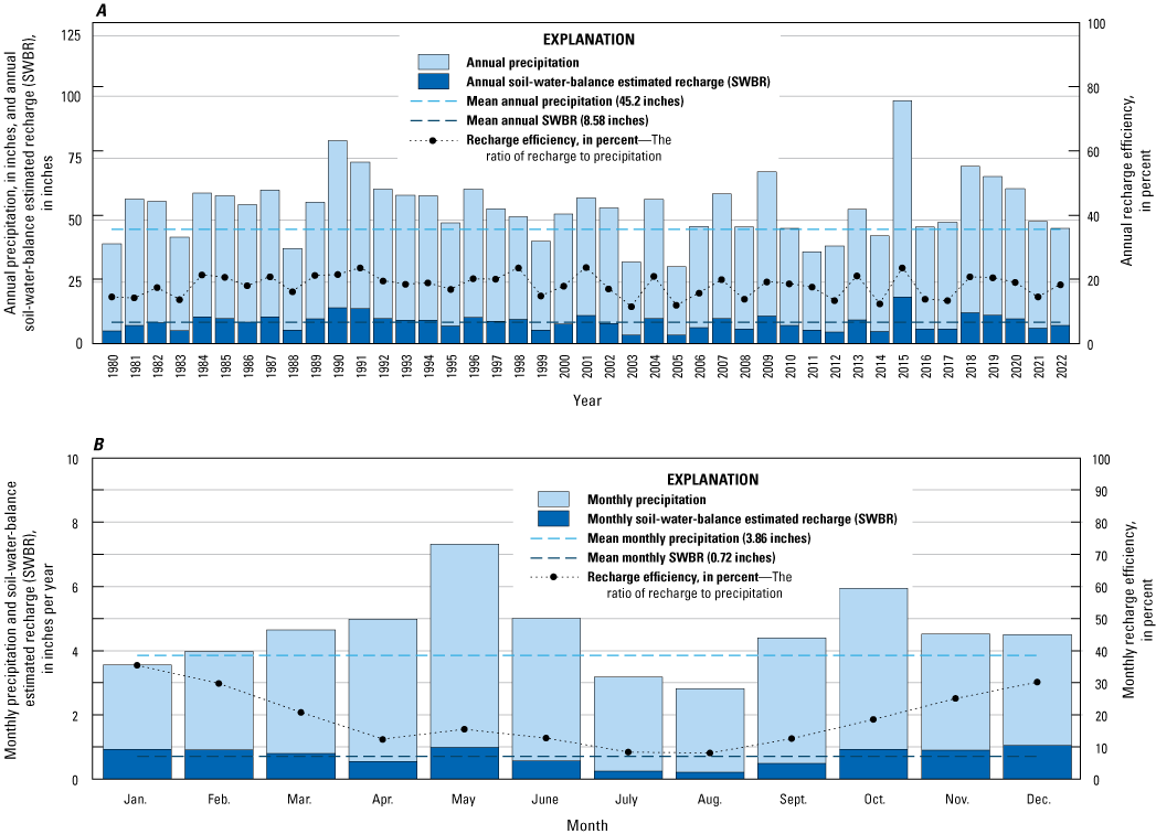
A, Annual precipitation and Soil-Water-Balance-estimated recharge (SWBR), and B, monthly precipitation and SWBR for the unconfined part of the Antlers aquifer, southeastern Oklahoma, 1980–2022.

Spatially distributed mean annual recharge computed using the Soil-Water-Balance code (Westenbroek and others, 2010) for the Antlers aquifer study area, southeastern Oklahoma, northeastern Texas, and southwestern Arkansas, 1980–2022.
The modeled SWBR rates were compared to published estimates of mean annual recharge rates for the Antlers aquifer. Morton (1992) estimated that recharge was between 0.32 and 0.96 in/yr. However, Morton (1992) estimated recharge as the net groundwater gain to the aquifer from stream seepage, which was calculated as gains or losses between streamflow measurement locations along streams. Morton (1992) did not account for the wider spatial distribution of recharge that occurs away from streams. This study used stream gain or loss measurements to calculate stream seepage similar to Morton (1992), but recharge was also estimated for spatial distribution of recharge across the Antlers aquifer by using the SWB method.
SWBR was used as the primary recharge estimate for the conceptual model because it is a model that accounts for multiple inputs over the entire aquifer, as opposed to local estimates. SWBR for the Antlers aquifer is estimated as an inflow of 799,252 acre-ft/yr and is the only net inflow to the aquifer (table 6).
Water-Table Fluctuation Method
The WTF method assumes that rises in groundwater levels that occur over a relatively short period of time (hours to days) in unconfined aquifers are attributable to recharge reaching the saturated zone following a period of precipitation. The WTF method is best suited for groundwater wells in areas with relatively shallow water tables and hydrographs from groundwater level observations from those wells that display sharp, rapid rises in groundwater levels in response to precipitation events. The WTF method requires knowledge or estimation of specific yield, which is often variable across the aquifer. A specific yield value is required in order to use the WTF method. Furthermore, the WTF method is used to estimate recharge for the area immediately surrounding the groundwater well in which water-level measurements are recorded. However, the properties of the aquifer at or near the well are not necessarily representative of the properties of the aquifer region-wide (Healy and Cook, 2002). The following equation is used in the WTF method to estimate annual recharge as the sum (∑) of individual water-level changes over time:
whereRa
is annual recharge, in inches per year;
Sy
is the specific yield of the aquifer, dimensionless;
Δh
is the change in water-level altitude, in inches; and
Δt
is the change in time, in years.
Water-level hydrographs from two USGS continuous water-level recorder wells (GW-01 and GW-06; fig. 7; table 1; USGS, 2023) were selected for the WTF method because these two wells were completed in the unconfined part of the Antlers aquifer and their hydrographs showed rapid responses to precipitation. Both wells were installed in the eastern part of the Antlers aquifer, where the mean annual precipitation is higher than in the western part. Because mean annual precipitation at the selected wells in the eastern part of the study area is relatively high, a greater annual recharge rate compared to the aquifer as a whole was likely. Nonetheless, the estimated percentage of precipitation that contributes to recharge can be applied to the rest of the Antlers aquifer. The water-level hydrographs from other continuous water-level recorder wells in the study area were excluded because they were either completed in the confined part of the aquifer (wells GW-02 and GW-04; fig. 1) or the hydrographs did not display adequate response to precipitation or were influenced by sources of recharge other than precipitation (wells GW-03 and GW-05; table 1).
Hart and Davis (1981) published a specific yield value of 0.17 for the Antlers aquifer, which was estimated from several aquifer tests; however, these aquifer tests typically lasted only a few hours. Short-duration aquifer tests tend to overestimate specific yield (Ferris and others, 1962), so the specific yield for the Antlers aquifer is likely lower. Jigmond and others (2014), who developed a groundwater availability model for the northern part of the Trinity aquifer in Texas (equivalent to the Antlers aquifer), used a specific yield value of 0.1; that Sy value was used to estimate recharge using the WTF method described in this report.
Annual precipitation data used for WTF for the 2013–22 period of analysis were calculated from daily precipitation values recorded at the nearest climate station to the selected well (fig. 1; table 7; NCEI, 2023; Oklahoma Mesonet, 2023). Using daily precipitation data from the nearest climate station and a specific yield of 0.1 (Jigmond and others, 2014), the mean annual recharge estimate for the period 2013–22 between GW-01 and GW-06 was 11.9 in/yr or 22.8 percent of mean annual precipitation normalized at each climate station for the period 1991–2020 (NCEI, 2023; Oklahoma Climatological Survey, 2021; table 7). The data were normalized by the mean annual recharge estimate (11.9 in/yr) and divided by the mean annual precipitation during 1991–2022. The WTF estimated recharge rate of 11.9 in/yr was used for comparison with the SWBR of 8.58 in/yr. The higher recharge rate estimated from the WTF method compared to the SWB method can be explained by the location of the wells used for the WTF method. All of the wells used in the WTF method were in the eastern part of the aquifer, where precipitation is higher than in the western part and higher than the overall mean precipitation rate for the Antlers aquifer (fig. 4; Thornton and others, 2020; Oklahoma Mesonet, 2023).
Table 7.
Summary of recharge estimates using the water-table fluctuation method for the Antlers aquifer, southeastern Oklahoma, 2013–22.[Dates shown as month, day, year. Data from continuous water-level recorder wells GW-02, GW-03, GW-04 and GW-05 were not suitable for analysis with the water-table-fluctuation method. All values are mean annualized values. --, not quantified]
| Descriptor | U.S. Geological Survey continuous water-level recorder well (fig. 1; table 1) | |
|---|---|---|
| GW-06 | GW-01 | |
| Mean annual precipitation 1991–2020, in inches, from nearby climate station(s) | 52.0 | 54.0 |
| Climate stations used | C-10, C-15 | C-07, C-12 |
| Estimated specific yield (Jigmond and others, 2014) | 0.10 | 0.10 |
| Annual precipitation, in inches | 49.5 | -- |
| Sum of water-level rises, in feet | 12.2 | -- |
| Recharge, in inches per year | 14.6 | -- |
| Recharge, percent of annual precipitation | 29.4 | -- |
| Recharge, in inches per year, normalized to mean annual precipitation, 1991–2020 | 15.3 | -- |
| Annual precipitation, in inches | 45.6 | -- |
| Sum of water-level rises, in feet | 5.3 | -- |
| Recharge, in inches per year | 6.3 | -- |
| Recharge, percent of annual precipitation | 13.9 | -- |
| Recharge, in inches per year, normalized to mean annual precipitation, 1991–2020 | 7.2 | -- |
| Annual precipitation, in inches | 47.5 | -- |
| Sum of water-level rises, in feet | 5.9 | -- |
| Recharge, in inches per year | 7.1 | -- |
| Recharge, percent of annual precipitation | 14.9 | -- |
| Recharge, in inches per year, normalized to mean annual precipitation, 1991–2020 | 7.7 | -- |
| Annual precipitation, in inches | 59.6 | -- |
| Sum of water-level rises, in feet | 6.8 | -- |
| Recharge, in inches per year | 8.1 | -- |
| Recharge, percent of annual precipitation | 13.6 | -- |
| Recharge, in inches per year, normalized to mean annual precipitation, 1991–2020 | 7.1 | -- |
| Annual precipitation, in inches | 55.2 | -- |
| Sum of water-level rises, in feet | 7.5 | -- |
| Recharge, in inches per year | 9.0 | -- |
| Recharge, percent of annual precipitation | 16.3 | -- |
| Recharge, in inches per year, normalized to mean annual precipitation, 1991–2020 | 8.5 | -- |
| Annual precipitation, in inches | 69.1 | -- |
| Sum of water-level rises, in feet | 9.9 | -- |
| Recharge, in inches per year | 11.9 | -- |
| Recharge, percent of annual precipitation | 17.1 | -- |
| Recharge, in inches per year, normalized to mean annual precipitation, 1991–2020 | 8.9 | -- |
| Annual precipitation, in inches | 49.5 | -- |
| Sum of water-level rises, in feet | 7.2 | -- |
| Recharge, in inches per year | 8.6 | -- |
| Recharge, percent of annual precipitation | 17.3 | -- |
| Recharge, in inches per year, normalized to mean annual precipitation, 1991–2020 | 9.0 | -- |
| Annual precipitation, in inches | 45.7 | 49.4 |
| Sum of water-level rises, in feet | 9.9 | 22.8 |
| Recharge, in inches per year | 11.9 | 27.3 |
| Recharge, percent of annual precipitation | 26.0 | 55.3 |
| Recharge, in inches per year, normalized to mean annual precipitation, 1991–2020 | 13.5 | 29.8 |
| Mean annual recharge during 2013–22, in inches per year, normalized to mean annual precipitation, 1991–2020 | -- | 11.9 |
Streambed Seepage
Streambed seepage is commonly estimated by making streamflow measurements during periods without precipitation runoff. Total streamflow is the sum of base flow and runoff into the stream from precipitation that falls on the drainage area. Base flow is the component of streamflow that is supplied by the discharge of groundwater to streams, whereas runoff is attributed to other factors such as precipitation and overland flow. Base flow can be measured directly in streams during periods when there is essentially no runoff component to streamflow (Garner and Bills, 2012). To directly measure base flow, a series of streamflow measurements were made for this study using the methods of Rantz (1982) during a period when the runoff component of streamflow was at or near 0 cubic feet per second, referred to hereinafter as “seepage run measurements.” The seepage-run measurements were collected at 23 sites within the spatial extent of the Antlers aquifer during January 17–18, 2023 (fig. 24). In addition to quantifying base flow at individual measurement sites, comparing measurements along a stream reach made it possible to delineate tributary inflow and outflow and to estimate streamflow gains and losses across the aquifer in January 2023.
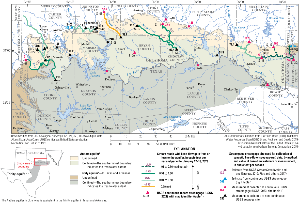
Seepage-run measurements and estimated base-flow gain and loss for selected streams that overlie the unconfined part of the Antlers aquifer, southeastern Oklahoma, January 17–18, 2023.
Seepage calculations along streams are done by subtracting inflow, including tributary inflow where applicable, from outflow and dividing this value by the total stream distance between measurement points. Seepage runs and estimates can help determine which stream reaches over the aquifer are gaining (that is, show a downstream increase in flow across the aquifer) or losing (that is, show a downstream decrease in flow across the aquifer). The stream lengths used in these calculations were obtained from the National Hydrography Dataset (Gary and others, 2009; Horizon Systems Corporation, 2015).
Tributaries with unmeasured base flows that were visually observed as having minimal or no flows were considered to contribute no base flow. Streamflow could not be measured in several tributaries that might have provided meaningful inflow data. Daily mean streamflow values measured during the same time period as the seepage run measurements from gaged locations on tributaries were used to supplement streamflow measurements obtained during seepage runs for the purpose of computed seepage gains and losses. Where gaged streamflow data or seepage-run measurements were not available, a seepage estimate was made by using a “zero-flow headwaters method.” The zero-flow headwaters method was done by estimating the length of the stream section from the furthest upstream measurement point up to the uppermost extent of the headwaters and assuming a gradient of increasing flow over the stream section assuming there was no flow at the uppermost extent of the headwaters. Thus, the seepage estimate was equal to the streamflow at the measurement point divided by the total upstream length of the stream from that point. This method was used to estimate streamflow for Walnut Bayou (figs. 1, 24; table 8). Another alternative method involved the use of USGS StreamStats (Smith and Esralew, 2010; Ries and others, 2017), which provided a watershed streamflow estimate to a selected point on the designated stream. This method was used to estimate streamflow for tributary inflow to the Little River in Arkansas (figs. 1, 24; table 8), as the zero-flow headwaters method was not viable owing to the large number of tributaries to this stream.
Table 8.
Summary streambed seepage estimations from base flow for the Antlers aquifer.[U.S. Geological Survey (USGS) values computed by using the Base-Flow Index code (Wahl and Wahl, 1995) in the USGS Groundwater Toolbox (Barlow and others, 2015). acre-ft/yr, acre-foot per year; n.d., not determined; --, not applicable]
| Stream section | Estimated streambed seepage calculations | |||||||||
|---|---|---|---|---|---|---|---|---|---|---|
| Upstream streamgage map identifier (fig. 1) | Mean base flow, 1980–2022 (acre-ft/yr) |
Upstream streamgage map identifier (fig. 1) |
Mean base flow, 1980–2022 (acre-ft/yr) |
Upstream streamgage map identifier (fig. 1) |
Mean base flow, 1980–2022 (acre-ft/yr) |
Downstream streamgage map identifier (fig. 1) |
Mean base flow, 1980–2022 (acre-ft/yr) |
Multi-plier1 | Net streambed seepage, 1980–2022 (acre-ft/yr) |
|
| 1 | S-12 | 94,479 | S-11 | 105,923 | -- | -- | S-13 | 302,503 | 0.9 | 91,890 |
| 2 | S-18 | 450,809 | S-19 | 236,693 | -- | 2146,191 | S-20 | 1,238,909 | 0.75 | 303,912 |
| 3 | S-08 | 53,957 | -- | -- | -- | -- | -- | 348,383 | 0.5 | −2,787 |
| 4 | -- | 4697,578 | -- | 512,683 | -- | 629,896 | S-02 | 905,945 | 0.7 | 116,052 |
| 5 | S-17 | 67,076 | -- | 7194,749 | -- | -- | S-18 | 450,809 | 0.8 | 151,186 |
| Total | -- | n.d. | -- | n.d. | -- | -- | -- | n.d. | -- | 660,253 |
Determined by estimating percentage of measured stream section that overlies the unconfined part of the Antlers aquifer.
Value estimated as percentage of flow determined from seepage run measurements, estimated to be 11.8 percent of measured flow at S-20.
Value estimated as percentage of flow determined from seepage run measurements, estimated to be 89.7 percent of measured flow at S-08.
Value estimated as percentage of flow determined from seepage run measurements, estimated to be 77 percent of measured flow at S-02.
Value estimated as percentage of flow determined from seepage run measurements, estimated to be 1.4 percent of measured flow at S-02.
Streamflow measurements across the unconfined part of the Antlers aquifer indicated that streams are net gaining across the study area (except for Blue River [fig. 24; tables 6, 8]), including the following: Red River, Walnut Bayou, Hickory Creek, part of the Washita River, Muddy Boggy Creek, and Little River. The longest measured base-flow net gaining stream reach was a 50.3-mi reach along the Red River overlying the far western part of the Antlers aquifer (fig. 24). The greatest base-flow gain (+2.27 cubic feet per second per mile) occurred over a 32.17-mi reach of the Little River (fig. 24).
Net streambed seepage for the conceptual model was estimated from mean annual base flows computed by using the BFI code (Wahl and Wahl, 1995) in the USGS Groundwater Toolbox (Barlow and others, 2015) on data from selected streamgages in the study area (figs. 1, 24; tables 2, 8). Base-flow values for streamgages immediately upstream from the measurement site and any other tributary inflows were subtracted from the base-flow of the downstream streamgage to calculate the total base flow fed to that stream reach and lost by the aquifer. The total gain or loss between the stream measurements was then multiplied by an approximate percentage of the stream that flowed over the unconfined part of the aquifer to account for net streambed seepage to the underlying aquifer (fig. 24; tables 6, 8). This estimation specifies the net base-flow gain from or loss to the aquifer. These estimates and calculations are summarized in tables 2 and 8. Net streambed seepage in the unconfined part of the Antlers aquifer for the period 1980–2022 is a net outflow from the Antlers aquifer of 660,253 acre-ft/yr or 82.6 percent of total outflow from the Antlers aquifer (tables 6, 8). Streambed seepage is estimated to be the largest contributor to outflow from the Antlers aquifer.
Lateral Groundwater Flows
No data were available to estimate lateral groundwater flows across the defined boundaries of the Antlers aquifer in Oklahoma. Lateral groundwater flows are assumed to be from flow across the aquifer from northwest to southeast as groundwater flows downgradient from Oklahoma into Texas and is pushed by the incoming recharge against the stagnant saline zone and out of the study area. Net lateral groundwater flow was calculated as the difference between the aquifer inflows (recharge) and the aquifer outflows (saturated-zone evapotranspiration, streambed seepage, and well withdrawals) and was used to balance the water budget. Net lateral groundwater flows for the Antlers aquifer in Oklahoma were estimated to be a net outflow of 128,355 acre-ft/yr or 16.1 percent of the overall water budget (table 6).
Saturated-Zone Evapotranspiration
Evapotranspiration is the process by which water is transferred to the atmosphere directly through evaporation and indirectly through plant transpiration. Most evapotranspiration occurs at or near the land surface where precipitation pools as surface water or where it infiltrates the soil unsaturated zone and becomes available to plant root zones; most precipitation does not reach the saturated zone of the aquifer (Lubczynski, 2009). The land-surface and unsaturated-zone components of evapotranspiration were not a part of the conceptual model for the Antlers aquifer because they occur before infiltrating precipitation has reached the saturated zone to become groundwater recharge. Saturated-zone evapotranspiration occurs in areas of the aquifer where the saturated zone intersects the plant-root zone, most commonly in lower lying or wetland areas along streams (Lubczynski, 2009). Saturated-zone evapotranspiration was an important part of the conceptual-model water budget.
Saturated-zone evapotranspiration is difficult to estimate over a large area such as the study area. However, saturated-zone evapotranspiration rates were assumed to be proportional to (1) the area where the saturated zone intersects the plant root zone, (2) the mean depth to groundwater in that area during the growing season, and (3) the mean rate of transpiration associated with the assemblage of plants in that area (Smith and others, 2021). Because saturated-zone evapotranspiration generally occurs in wetland areas, wetland data from the National Wetlands Inventory (U.S. Fish and Wildlife Service, 2014) were used to determine the total area of wetlands overlying the unconfined part of the Antlers aquifer. Land areas with frequently saturated or flooded soils are classified as wetlands (Cowardin and others, 1979). An estimated 42,965 acres of wetland area (about 4 percent of the total unconfined area) overlie the unconfined part of the Antlers aquifer. The saturated-zone component of evapotranspiration was assumed to be active during the growing season (April–October [National Agricultural Statistics Service, 2023; Oklahoma Climatological Survey, 2023]). On an annual and monthly basis, the saturated-zone component of evapotranspiration is greatest in wet and hot years, and greatest in early summer months when precipitation and temperature are above their mean annual values (figs. 4, 5, 22; Scholl and others, 2005). In an earlier groundwater flow model for the Antlers aquifer, Morton (1992) concluded that evapotranspiration from the saturated zone was a trivial component of the overall water budget because the depth of the water table (about 50 ft below land surface) was deep enough to eliminate any concerns about saturated-zone evapotranspiration contributing to groundwater losses from the Antlers aquifer. Modeling tools have improved since 1992, and for this assessment, evapotranspiration from the shallower parts of the water table along streams and wetlands overlying the unconfined part of the aquifer was considered in the computation of the water budget.
White (1932) estimated annual saturated-zone evapotranspiration rates of 0.75–1.9 ft/yr for undisturbed Distichlis spicata (saltgrass) cover in southwestern Utah with a mean depth to water of 1–2 ft. Relative humidity and dewpoint temperature are comparatively low in southwestern Utah compared to southeastern Oklahoma (National Climatic Data Center, 2023); however, precipitation is much higher in southeastern Oklahoma compared to southwestern Utah, which likely results in an overall higher annual rate of evapotranspiration for the study area compared to what White (1932) reported for his study area. Smith and others (2021) and Rogers and others (2023) estimated saturated-zone evapotranspiration for the Salt Fork of the Red River alluvial aquifer and reaches 3 and 4 of the Washita River alluvial aquifer to be 1 ft/yr and 1.33 ft/yr, respectively. These two aquifers are in southwestern Oklahoma, where mean precipitation rates are lower than they are in southeastern Oklahoma. Although the methods described in White (1932) account for the WTF method assumptions described in this section of the report, annual data that covered the entire study period (1980–2022) were not available from any of the shallow wells. Thus, the White (1932) methods were not used in this report to estimate groundwater outflows attributable to saturated-zone evapotranspiration from daily WTF data at wells with shallow depths to water. Wells GW-01, GW-04, and GW-06 (fig. 1; table 1) each show some level of daily fluctuation during the daylight hours in the summer months (fig. 7). These daily fluctuations are indicative of daily declines in groundwater level during daylight hours in summer conditions. The observation of these daily fluctuations in groundwater levels indicated that saturated-zone evapotranspiration was an active process in the Antlers aquifer. Because the unconfined part of the Antlers aquifer receives greater amounts of precipitation (Oklahoma Mesonet, 2023) and is generally warmer than the areas overlying the Salt Fork of the Red River alluvial aquifer and reaches 3 and 4 of the Washita River alluvial aquifer, a saturated-zone evapotranspiration rate of 2.0 ft/yr was assumed for the study area. If the estimated 42,965 acres of wetland area that overlie the unconfined part of the Antlers aquifer are assumed to have a constant depth to water and saturated-zone evapotranspiration rate, the saturated-zone evapotranspiration rate would correspond to an annual saturated-zone evapotranspiration outflow of 7,161 acre-ft/yr or 0.9 percent of outflow from the Antlers aquifer (fig. 21; table 6).
Well Withdrawals
Well withdrawals were assumed to be equivalent to the mean annual reported groundwater use during 1980–2022, or 3,483 acre-ft/yr (fig. 21; tables 3, 5, 6). These withdrawals were generally greatest during dry and hot years because more groundwater was required in those years for crops to make up for the lack of precipitation and increased evapotranspiration. The altitude of the water table generally declines during dry and hot years (especially during extended droughts) and rises during wet and cool years (figs. 4, 7). The degree to which the water table fluctuates annually at a given location is related in part to the volume of nearby well withdrawals and the distribution (or concentration) of recharge near that location. The well withdrawal amount of 3,483 acre-ft/yr for the study period accounts for 0.4 percent of the conceptual water budget (fig. 21; table 6).
Vertical Leakage
Groundwater exchange is probably substantial between the Antlers aquifer and the Goodland-Walnut confining unit (Hart and Davis, 1981) but probably not substantial between the Antlers aquifer and the lower confining units. Groundwater exchange likely involves groundwater inflow to the Antlers aquifer from the overlying Goodland-Walnut confining unit in the shallow parts of the confined Antlers aquifer; the direction of groundwater flow eventually reverses from inflow to outflow as the altitude of the top of the Antlers aquifer decreases. The hydrograph from continuous water-level recorder well GW-02 (fig. 7C; USGS, 2023), which is completed in the confined part of the Antlers aquifer, shows rapid responses to precipitation, indicating that the Antlers aquifer is vertically hydraulically connected to the overlying units and that vertical leakage is occurring. The observed response to precipitation could also be an effect of site-specific issues with the given well, such as compromised well casings or surface seals designed to keep surface runoff from entering the well. Because of the change from groundwater inflow to outflow with depth, net vertical leakage is considered to be net zero and a negligible part of the water budget (fig. 21; table 6).
Groundwater Storage
Annual water-level measurements for the 1980–2022 study period were not available from wells completed in the Antlers aquifer, so estimating net storage change in the aquifer was not possible. The net storage change of the Antlers aquifer was assumed to be a negligible component of the conceptual-model water budget (fig. 21; table 6), which corresponds with the minimal change between the potentiometric maps in Hart and Davis (1981) and Morton (1992) and in this report.
Conceptual Water Budget
The conceptual-model water budget (table 6) summarized mean water inflows and outflows exchanged between each hydrologic boundary of the Antlers aquifer for the 1980–2022 study period. Hydrologic boundaries of the water budget were estimated by analyzing the available data; however, where data were not available, assumptions were made by using published analogs. Recharge accounts for 82.6 percent of the conceptual-model inflows to the Antlers aquifer, and net streambed seepage accounts for 100 percent of the outflows from the Antlers aquifer. Net lateral groundwater flow (16.1 percent of outflows), saturated-zone evapotranspiration (0.9 percent of outflows), and well withdrawals (0.4 percent of outflows) were the only other components estimated to contribute to the water budget (table 6). Vertical leakage and changes in storage were considered to be negligible components of the conceptual water budget. The balanced total inflows and outflows for the Antlers aquifer were estimated as 799,252 acre-ft/yr for the 1980–2022 study period (table 6). Morton (1992) developed a water-budget for a transient model simulation from 1911 to 1970 with an estimated annual inflow of 98,034 acre-ft/yr, an outflow of 98,230 acre-ft/yr, and a net annual loss in water storage of 196 acre-ft/yr. The values estimated in Morton (1992) were estimated by using different methods compared to the methods used in this report.
Summary
The 1973 Oklahoma Water Law (Oklahoma Statute §82–1020.5) requires that the Oklahoma Water Resources Board (OWRB) conduct hydrologic investigations of the State’s aquifers (called “groundwater basins” in the statutes) to support a determination of the maximum annual yield (MAY) for each aquifer. The MAY is defined as the amount of fresh groundwater that can be withdrawn annually while ensuring a minimum 20-year life of the aquifer. Groundwater with a total dissolved solids concentration of less than 5,000 milligrams per liter or less is considered fresh in Oklahoma. For bedrock aquifers, the groundwater-basin-life requirement is satisfied if, after 20 years of MAY withdrawals, 50 percent of the groundwater basin (hereinafter referred to as an “aquifer”) retains a saturated thickness of at least 15 feet. Although 20 years is the minimum required by law, the OWRB can and often does consider multiple management scenarios. The annual volume of water allocated to that groundwater permit applicant is determined once a MAY has been established and is dependent on the amount of land owned or leased by a permit applicant. The MAY is divided by the total land area overlying the aquifer to determine the annual volume of groundwater allocated per acre of land, or the equal-proportionate-share (EPS) pumping rate. The OWRB issued a final order on February 14, 1995, that established a MAY of 5,913,600 acre-feet per year (acre-ft/yr) and an EPS pumping rate of 2.1 acre-feet per acre per year for the Antlers aquifer. Because more than 20 years have elapsed since the final order was issued, the U.S. Geological Survey (USGS), in cooperation with the OWRB, updated the hydrogeologic framework and developed a conceptual groundwater-flow model as part of the hydrologic investigation of the Antlers aquifer for updating the MAY and EPS pumping rates for a 1980–2022 study period.
An updated hydrogeologic framework for the Antlers aquifer was developed that included refining the aquifer boundary in Oklahoma, the creation of new potentiometric surface and saturated thickness of fresh groundwater maps, one multiple-well aquifer test, slug tests, and an analysis of lithologic logs across the aquifer. The hydrogeologic framework for the Antlers aquifer included updated definitions of the aquifer extent and potentiometric surface, as well as a description of the hydraulic and textural properties of aquifer materials. A conceptual groundwater flow model and water budget were developed by incorporating estimates of recharge from precipitation, saturated-zone evapotranspiration, streambed seepage, lateral groundwater flows, vertical leakage, and withdrawals from groundwater wells.
The distribution and variability of hydraulic and textural properties of the Antlers aquifer, especially the horizontal hydraulic conductivity, were assumed to be the primary controls on groundwater flow. Multiple methods were used to estimate the range and central tendency of horizontal hydraulic conductivity values in the aquifer. These methods included a multiple-well aquifer test, slug tests, and analysis of lithologic descriptions from wells completed in the Antlers aquifer. Horizontal hydraulic conductivity was estimated to range from 0.87 to 10.65 feet per day with a mean value of 3.31 feet per day. Transmissivity was estimated to range from 399 to 6,416 square feet per day. The storage coefficient ranged from 0.0006 to 0.004 for the confined part of the Antlers aquifer, whereas the unconfined part ranged from 0.10 to 0.11, which was determined by applying the specific yield obtained from the literature (0.1) for the Trinity aquifer to the slug test results. Specific storage was estimated to range from 1.1 × 10⁻⁶ to 5.0 × 10⁻⁵. The estimated total groundwater storage for the Antlers aquifer ranged from about 120,000,000 to 156,000,000 acre-feet.
Two key components for simulating a groundwater-flow system are the conceptual groundwater flow model (hereinafter referred to as the “conceptual model”) and the resulting water budget. A conceptual model is a simplified representation of the groundwater-flow system that accounts for the major inflows and outflows across hydrologic boundaries into a water budget. A conceptual model is thus the means for approximating the water budget for an aquifer. Hydrologic boundaries are boundaries based on the hydrogeologic framework, hydrologic controls, and climatic conditions where water flows into or out of the aquifer, thus potentially changing the total storage of the aquifer.
The conceptual model for the Antlers aquifer provided a water budget that was used to quantify net groundwater flows across each identified hydrologic boundary for the Antlers aquifer for the 1980–2022 study period. Estimated recharge to the Antlers aquifer, determined by means of the Soil-Water Balance code, was 8.58 inches per year or 19 percent of the mean annual precipitation for the 1980–2022 study period. The mean annual recharge rate for the unconfined part of the Antlers aquifer was 799,252 acre-ft/yr to the aquifer. Streambed seepage was estimated by using data from USGS streamgages to calculate base flow over the unconfined part of the Antlers aquifer using a combination of seepage-run measurements, USGS StreamStats, and base-flow-index estimates. Seepage estimates indicate that streams were gaining over the unconfined part of the aquifer, meaning that there is a net loss from the aquifer. Streamflow seepage was the largest outflow from the Antlers aquifer, with a net outflow of 660,253 acre-ft/yr for the 1980–2022 period. Net lateral groundwater flow is unknown, and no methods were employed in this study to measure this value. Net lateral groundwater flow was used to balance the conceptual water budget and was considered to be a net outflow from the Antlers aquifer of 128,355 acre-ft/yr. An estimated 42,965 acres of wetlands overlie the unconfined part of the Antlers aquifer in Oklahoma, where saturated-zone evapotranspiration was assumed to occur. These wetlands are generally located along streams where the water table is close to the land surface. The saturated-zone evapotranspiration rate estimated for the study area was 2.0 feet per year. Saturated-zone evapotranspiration for the wetland areas that overlie the unconfined part of the Antlers aquifer in Oklahoma was estimated to account for an outflow from the aquifer of 7,161 acre-ft/yr. Well withdrawals from the Antlers aquifer were estimated from the mean annual reported groundwater use during 1980–2022, which accounted for an outflow from the aquifer of 3,483 acre-ft/yr. Vertical leakage is unknown and no methods were employed for this study to measure this value. Vertical leakage and change in storage were considered to be negligible parts of the Antlers aquifer conceptual water budget. The balanced total inflows and outflows for the Antlers aquifer were estimated to be 799,252 acre-ft/yr for the 1980–2022 study period.
References Cited
Alley, W.M., Reilly, T.E., and Franke, O.L., 1999, Sustainability of ground-water resources: U.S. Geological Survey Circular 1186, 79 p., accessed April 1, 2024, at https://doi.org/10.3133/cir1186.
Ashworth, J.B., and Hopkins, J., 1995, Aquifers of Texas: Texas Water Development Board Report 345, p. 18–19, accessed December 15, 2024, at https://www.twdb.texas.gov/publications/reports/numbered_reports/doc/R345/R345Complete.pdf.
Barlow, P.M., Cunningham, W.L., Zhai, T., and Gray, M., 2015, U.S. Geological Survey groundwater toolbox, a graphical and mapping interface for analysis of hydrologic data (version 1.0)—User guide for estimation of base flow, runoff, and groundwater recharge from streamflow data: U.S. Geological Survey Techniques and Methods, book 3, chap. B10, 27 p., accessed November 2, 2023, at https://doi.org/10.3133/tm3B10.
Barlow, P.M., and Leake, S.A., 2012, Streamflow depletion by wells—Understanding and managing the effects of groundwater pumping on streamflow: U.S. Geological Survey Circular 1376, 84 p., accessed December 12, 2023, at https://doi.org/10.3133/cir1376.
Bouwer, H., and Rice, R.C., 1976, A slug test for determining hydraulic conductivity of unconfined aquifers with completely or partially penetrating wells: Water Resources Research, v. 12, no. 3, p. 423–428, accessed December 16, 2023, at https://doi.org/10.1029/WR012i003p00423.
Chang, J.M., and Stanley, T.M., 2013, Preliminary geologic map of the Tishomingo 30′ × 60′ quadrangle and the Oklahoma part of the Sherman 30′ × 60′ quadrangle, Atoka, Bryan, Carter, Choctaw, Coal, Johnston, Love, Marshall, Murray, and Pontotoc Counties, Oklahoma: Oklahoma Geological Survey Oklahoma Geologic Quadrangle OGQ-88, scale 1:100,000, accessed August 3, 2022, at http://ogs.ou.edu/docs/OGQ/OGQ-88-color.pdf.
Cowardin, L.M., Carter, V., Golet, F.C., and LaRoe, E.T., 1979, Classification of wetlands and deepwater habitats of the United States: Washington, D.C., U.S. Department of the Interior, U.S. Fish and Wildlife Service, 131 p., accessed December 6, 2023, at https://www.epa.gov/sites/default/files/2017-05/documents/cowardin_1979.pdf.
Davis, L.V., 1960, Geology and ground-water resources of southern McCurtain County, Oklahoma: Oklahoma Geological Survey Bulletin 86, 108 p., accessed June 11, 2024, at http://ogs.ou.edu/docs/bulletins/B86.pdf.
Duffield, G.M., 2025, Representative values of hydraulic properties: AQTESOLV web page, accessed February 4, 2025, at http://www.aqtesolv.com/pumping-tests/recovery-tests.htm.
Ellis, J.H., Mashburn, S.L., Graves, G.M., Peterson, S.M., Smith, S.J., Fuhrig, L.T., Wagner, D.L., and Sanford, J.E., 2017, Hydrogeology and simulation of groundwater flow and analysis of projected water use for the Canadian River alluvial aquifer, western and central Oklahoma (ver. 1.1, March 2017): U.S. Geological Survey Scientific Investigations Report 2016–5180, 64 p., 7 pls., accessed June 11, 2024, at https://doi.org/10.3133/sir20165180.
Esri, 2023, ArcGIS for desktop help—Fill tool: Esri web page, accessed December 12, 2023, at https://desktop.arcgis.com/en/arcmap/10.7/tools/spatial-analyst-toolbox/fill.htm.
Ferris, J.G., Knowles, D.B., Browne, R.H., and Stallman, R.W., 1962, Theory of aquifer tests: U.S. Geological Survey Water-Supply Paper 1536-E, 167 p., accessed June 11, 2024, at https://doi.org/10.3133/wsp1536E.
Fetkovich, E.J., Baciocco, A.B., Dale, I.A., Rogers, I.M.J., Wagner, D.L., Tomlinson, Z., and Fiorentino, E.G., 2025, Soil water balance model and data used in the hydrogeologic investigation, framework, and conceptual flow model of the Antlers aquifer, southeastern Oklahoma, 1967–2022: U.S. Geological Survey data release, https://doi.org/10.5066/P14C6QFS.
Frederickson, E.A., Redman, R.H., and Westheimer, J.M., 1965, Geology and petroleum of Love County, Oklahoma: Oklahoma Geological Survey Circular 63, 91 p., accessed December 15, 2023, at http://www.ogs.ou.edu/pubsscanned/Circulars/Circular63mm.pdf.
Garner, B.D., and Bills, D.J., 2012, Spatial and seasonal variability of base flow in the Verde Valley, central Arizona, 2007 and 2011: U.S. Geological Survey Scientific Investigations Report 2012–5192, 33 p., accessed December 12, 2023, at https://doi.org/10.3133/sir20125192.
Gary, R.H., Wilson, Z.D., Archuleta, C.M., Thompson, F.E., and Vrabel, J., 2009, Production of a national 1:1,000,000-scale hydrography dataset for the United States—Feature selection, simplification, and refinement (revised May 2010): U.S. Geological Survey Scientific Investigations Report 2009–5202, 22 p., accessed April 18, 2024, at https://doi.org/10.3133/sir20095202.
George, P.G., Mace, R.E., and Petrossian, R., 2011, Aquifers of Texas: Texas Water Development Board Report 380, p. 67–72, accessed February 11, 2025, at https://www.twdb.texas.gov/publications/reports/numbered_reports/index.asp.
Greenlee, D.D., 1987, Raster and vector processing for scanned linework: Photogrammetric Engineering and Remote Sensing, v. 53, no. 10, p. 1383–1387, accessed December 16, 2023, at https://www.asprs.org/wp-content/uploads/pers/1987journal/oct/1987_oct_1383-1387.pdf.
Groundwater Protection Council, 2015, Produced water reuse in Oklahoma—Regulatory considerations and references: Groundwater Protection Council, 51 p., accessed December 16, 2023, at https://www.gwpc.org/wp-content/uploads/2022/12/Oklahoma_Produced_Water_Project_Summary_Report.pdf.
Haley, B.R., Glick, E.E., Bush, W.V., Clardy, B.F., Stone, C.G., Woodward, M.J., and Zachry, D.L., 1993, Geologic map of Arkansas: Arkansas Geologic Commission and U.S. Geological Survey [unnumbered report], 1 plate, accessed April 18, 2024, at https://doi.org/10.3133/70210562.
Halford, K.J., and Kuniansky, E.L., 2002, Documentation of spreadsheets for the analysis of aquifer-test and slug-test data: U.S. Geological Survey Open File Report 2002–197, 54 p., accessed January 17, 2025, at https://pubs.usgs.gov/of/2002/ofr02197/documentation.pdf.
Handson, W.D., Clardy, B.F., Haley, B.R., Stone, C.G., and Perkins, J.R., 1999, Geologic map of the Chapel Hill quadrangle, Sevier County, Arkansas: Arkansas Geological Commission Digital Geologic Quadrangle Map DGM-AR-00149, scale 1:24,000, accessed February 11, 2025, at https://www.geology.arkansas.gov/docs/pdf/maps-and-data/geologic_maps/24k/Chapel%20Hill.pdf.
Hantush, M.S., 1960, Modification of the theory of leaky aquifers: Journal of Geophysical Research, v. 65, no. 11, p. 3713–3725, accessed April 28, 2024, at https://agupubs.onlinelibrary.wiley.com/doi/epdf/10.1029/JZ065i011p03713.
Hargreaves, G.H., and Samani, Z.A., and the George H. Hargreaves, and the Zohrab A. Samani, 1985, Reference crop evapotranspiration from temperature: Applied Engineering in Agriculture, v. 1, no. 2, p. 96–99, accessed December 12, 2023, at https://doi.org/10.13031/2013.26773.
Hart, D.L., Jr., and Davis, R.E., 1981, Geohydrology of the Antlers aquifer (Cretaceous), southeastern Oklahoma: Oklahoma Geological Survey Circular 81, 33 p., accessed December 16, 2024, at http://www.ogs.ou.edu/pubsscanned/Circulars/circular81mm.pdf.
Healy, R.W., and Cook, P.G., 2002, Using groundwater levels to estimate recharge: Hydrogeology Journal, v. 10, no. 1, p. 91–109, accessed December 12, 2023, at https://doi.org/10.1007/s10040-001-0178-0.
Heran, W.D., Green, G.N., and Stoeser, D.B., 2003, A digital geologic map database for the State of Oklahoma: U.S. Geological Survey Open-File Report 03–247, 10 p., accessed December 12, 2023, at https://doi.org/10.3133/ofr03247.
Horizon Systems Corporation, 2015, National Hydrography Dataset Plus (NHDPlus) version 1: Horizon Systems Corporation database, accessed June 6, 2023, at https://nhdplus.com/NHDPlus/.
Huffman, G.G., Alfonsi, P.P., and Dalton, R.C., Duarte-Vivas, A., and Jeffries, E.L., 1975, Geology and mineral resources of Choctaw County, Oklahoma: Oklahoma Geological Survey Bulletin 120, 39 p., accessed May 10, 2024, at http://www.ogs.ou.edu/pubsscanned/BULLETINS/Bulletin120mm.pdf.
Hvorslev, M.J., 1951, Time lag and soil permeability in ground-water observations: Vicksburg, Miss., U.S. Army Corps of Engineers Waterways Experiment Station Bulletin no. 36, 50 p., accessed March 29, 2024, at https://apps.dtic.mil/sti/trecms/pdf/ADA950075.pdf.
Hyder, Z., Butler, J.J., Jr., McElwee, C.D., and Liu, W., 1994, Slug tests in partially penetrating wells: Water Resources Research, v. 30, no. 11, p. 2945–2957, accessed May 28, 2024, at https://doi.org/10.1029/94WR01670.
Hydrosolve, Inc., 2011, Aqtesolv for windows: Hydrosolve, Inc. website, accessed June 1, 2023, at http://www.aqtesolv.com/.
Jigmond, M., Harding, J., Pinkard, J., Yan, T.T., Scanlon, B., Reedy, B., Beach, J., Davidson, T., and Laughlin, K., 2014, Updated groundwater availability model of the northern Trinity and Woodbine aquifers: Texas Water Development Board report, v. 1, p. 6.4–4, accessed December 15, 2024, at https://www.twdb.texas.gov/groundwater/models/gam/trnt_n/Final_NTGAM_Vol%20I%20Aug%202014_Report.pdf?d=4535.3850000028615.
Kottek, M., Grieser, J., Beck, C., Rudolf, B., and Rubel, F., 2006, World map of the Kӧppen-Geiger climate classification updated: Meteorologische Zeitschrift (Berlin), v. 15, no. 3, p. 259–263, accessed February 2, 2024, at https://doi.org/10.1127/0941-2948/2006/0130.
Kuniansky, E.L., Jones, S.A., Brock, R.D., and Williams, M.D., 1996, Hydrogeology at Air Force Plant 4 and vicinity and water quality of the Paluxy aquifer, Fort Worth, Texas: U.S. Geological Survey Water-Resources Investigations Report 96–4091, 1 p., accessed December 15, 2023, at https://doi.org/10.3133/wri964091.
Lohman, S.W., 1972, Groundwater hydraulics: U.S. Geological Survey Professional Paper 708, 70 p., accessed April 2, 2024, at https://doi.org/10.3133/pp708.
Lubczynski, M.W., 2009, The hydrogeological role of trees in water-limited environments: Hydrogeology Journal, v. 17, no. 1, p. 247–259, accessed December 12, 2023, at https://doi.org/10.1007/s10040-008-0357-3.
Marcher, M.V., and Bergman, D.L., 1983, Reconnaissance of the water resources of the McAlester and Texarkana quadrangles, southeastern Oklahoma: Oklahoma Geological Survey Hydrologic Atlas HA-9, 4 sheets, scale 1:250,000, accessed May 29, 2024, at https://ngmdb.usgs.gov/Prodesc/proddesc_16317.htm.
Mashburn, S.L., Ryter, D.W., Neel, C.R., Smith, S.J., and Correll, J.S., 2014, Hydrogeology and simulation of groundwater flow in the Central Oklahoma (Garber-Wellington) aquifer, Oklahoma, 1987 to 2009, and simulation of available water in storage, 2010–2059 (ver. 2.0, October 2019): U.S. Geological Survey Scientific Investigations Report 2013–5219, 92 p., accessed December 12, 2023, at https://doi.org/10.3133/sir20135219.
Miser, H.D., and Purdue, A.H., 1919, Gravel deposits of the Caddo Gap and De Queen Quadrangles, Arkansas: U.S. Geological Survey Bulletin 690-B, p. 15–29, accessed February 12, 2025, at https://pubs.usgs.gov/bul/0690b/report.pdf.
Moix, M.W., and Galloway, J.M., 2005, Base flow, water quality, and streamflow gain and loss of the Buffalo River, Arkansas, and selected tributaries, July and August 2003: U.S. Geological Survey Scientific Investigations Report 2004–5274, 36. p., accessed April 1, 2023, at https://doi.org/10.3133/sir20045274.
Morton, R.B., 1992, Simulation of ground-water flow in the Antlers aquifer in southeastern Oklahoma and northeastern Texas: U.S. Geological Survey Water-Resources Investigations Report 88–4208, 22 p., accessed December 12, 2023, at https://doi.org/10.3133/wri884208.
Multi-Resolution Land Characteristics Consortium, 2023, National Land Cover Database (NLCD) 2016: Multi-Resolution Land Characteristics Consortium database, accessed May 28, 2024, at https://www.mrlc.gov/data/nlcd-2016-land-cover-conus.
National Agricultural Statistics Service, 2023, Oklahoma agricultural statistics 2022: National Agricultural Statistics Service, Oklahoma Department of Agriculture, Food, and Forestry, Oklahoma Annual Statistical Bulletin 2020 edition, 84 p., accessed December 16, 2023, at https://www.nass.usda.gov/Statistics_by_State/Oklahoma/Publications/Annual_Statistical_Bulletin/ok-bulletin-2020-web-versionupdatedlinks.pdf.
National Atlas of the United States, 2014, Global map—Cities and towns of the United States, 2014: National Atlas of the United States, accessed December 18, 2023, at https://earthworks.stanford.edu/catalog/stanford-nh933kw1202.
National Centers for Environmental Information [NCEI], 2023, Daily observational data—GHCN daily: National Oceanic and Atmospheric Administration database, accessed August 10, 2023, at https://www.ncei.noaa.gov/maps/daily/.
National Climatic Data Center, 2023, National Weather Service online weather data: National Weather Service database accessed June 8, 2023, at https://www.weather.gov/wrh/Climate?wfo=tsa.
Oklahoma Climatological Survey, 2021, Climate of Oklahoma normal annual precipitation map: Oklahoma Climatological Survey webpage, accessed January 15, 2025, at https://www.ou.edu/ocs/oklahoma-climate.
Oklahoma Climatological Survey, 2023, Climate of Oklahoma average length of growing season map: Oklahoma Climatological Survey webpage, accessed January 15, 2025, at https://www.ou.edu/ocs/oklahoma-climate.
Oklahoma Mesonet, 2023, Daily data retrieval: Oklahoma Mesonet web page, accessed July 2023, at https://www.mesonet.org/index.php/past_data/daily_data_retrieval.
Oklahoma State Legislature, 2021a, Determination of maximum annual yield, chap. 1020, section 5 of Waters and water rights: Oklahoma Statutes, title 82, accessed October 19, 2021, at https://oksenate.gov/sites/default/files/2019-12/os82.pdf.
Oklahoma State Legislature, 2021b, Definitions, chap. 1020, section 1 of Waters and water rights: Oklahoma Statutes, title 82, accessed October 19, 2021, at https://oksenate.gov/sites/default/files/2019-12/os82.pdf.
Oklahoma State Legislature, 2021c, Domestic use—Spacing of wells and waste, chap. 1020, section 3 of Waters and water rights: Oklahoma Statutes, title 82, accessed October 19, 2021, at https://oksenate.gov/sites/default/files/2019-12/os82.pdf.
Oklahoma Water Resources Board [OWRB], 2012, Oklahoma comprehensive water plan—Executive report (updated 2012): Oklahoma Water Resources Board, 151 p., accessed January 15, 2025, at https://oklahoma.gov/content/dam/ok/en/owrb/documents/water-planning/ocwp/OCWPExecutiveRpt.pdf.
Oklahoma Water Resources Board [OWRB], 2018, 2018 Oklahoma groundwater report—Beneficial use monitoring program: Oklahoma Water Resources Board, 84 p., accessed February 5, 2025, at https://oklahoma.gov/content/dam/ok/en/owrb/documents/maps-and-data/water-monitoring/oklahoma-groundwater-monitoring-report.pdf.
Oklahoma Water Resources Board [OWRB], 2023a, Maximum annual yield: Oklahoma Water Resources Board Fact Sheet, 2 p., accessed December 2023, at https://oklahoma.gov/content/dam/ok/en/owrb/documents/science-and-research/hydrologic-investigations/maximum-annual-yield-determinations-fact-sheet.pd f.
Oklahoma Water Resources Board [OWRB], 2023b, OWRB water use permits in Oklahoma: Oklahoma Water Resources Board database, accessed December 16, 2023, at https://www.owrb.ok.gov/maps/PMG/owrbdata_WR.html.
Oklahoma Water Resources Board [OWRB], 2023c, Taking and use of groundwater: Oklahoma Water Resources Board Title 785, chap. 30, 449 p., accessed December 16, 2023, at https://oklahomarules.blob.core.windows.net/titlepdf/Title_785.pdf.
Oklahoma Water Resources Board [OWRB], 2023d, Interactive maps and GIS data: Oklahoma Water Resources Board database, accessed December 16, 2023, at https://oklahoma.gov/owrb/data-and-maps/interactive-maps.html.
Oklahoma Water Resources Board [OWRB], 2023e, OWRB open data—Groundwater: Oklahoma Water Resources Board database, accessed November 10, 2023, at https://home.owrb.opendata.arcgis.com/search?tags=groundwater.
Oklahoma Water Resources Board [OWRB], 2024, Oklahoma groundwater resources—Major and minor aquifers of Oklahoma: Oklahoma Water Resources Board web map, accessed January 20, 2024, at https://www.owrb.ok.gov/maps/pdf_map/GW%20Aquifers.pdf.
Oklahoma Water Resources Board [OWRB], 2025, Water permitting: Oklahoma Water Resources Board Fact Sheet, 1 p., accessed January 14, 2025, at https://oklahoma.gov/content/dam/ok/en/owrb/documents/water-permitting/water-permitting-fact-sheet.pdf.
Piper, A.M., 1944, A graphic procedure in the geochemical interpretation of water analyses: Transactions - American Geophysical Union, v. 25, no. 6, p. 914–928, accessed July 8, 2023, at https://doi.org/10.1029/TR025i006p00914.
Rantz, S.E., 1982, Measurement and computation of streamflow—Volume 1. Measurement of stage and discharge: U.S. Geological Survey Water-Supply Paper 2175, 284 p., accessed June 8, 2023, at https://doi.org/10.3133/wsp2175.
Ries, K.G., III, Newson, J.K., Smith, M.J., Guthrie, J.D., Steeves, P.A., Haluska, T.L., Kolb, K.R., Thompson, R.F., Santoro, R.D., and Vraga, H.W., 2017, StreamStats, version 4: U.S. Geological Survey Fact Sheet 2017–3046, 4 p., accessed June 5, 2020, at https://doi.org/10.3133/fs20173046.
Robinson, M.C., and Deeds, N.E., 2019, Identification of potential brackish groundwater production areas—Northern Trinity aquifer: Texas Water Development Board Technical Note 19-1, 132 p., accessed June 7, 2023, at https://www.twdb.texas.gov/groundwater/bracs/studies/Northern_Trinity/index.asp#finalreport.
Rogers, I.M.J., Smith, S.J., Gammill, N.C., Gillard, N.J., Lockmiller, K.A., Fetkovich, E.J., Correll, J.S., and Hussey, S.P., 2023, Hydrogeology and simulated groundwater availability in reaches 3 and 4 of the Washita River aquifer, 1980–2017: U.S. Geological Survey Scientific Investigations Report 2023–5072, 83 p., accessed December 16, 2023, at https://doi.org/10.3133/sir20235072.
Ryder, P.D., 1996, Ground water Atlas of the United States—Segment 4, Oklahoma, Texas: U.S. Geological Survey Hydrologic Atlas 730-E, p. 19–25, accessed November 1, 2023, at https://doi.org/10.3133/ha730E.
Scholl, M., Christenson, S., Cozzarelli, I., Ferree, D., and Jaeshke, J., 2005, Recharge processes in an alluvial aquifer riparian zone, Norman Landfill, Norman, Oklahoma, 1998–2000: U.S. Geological Survey Scientific Investigations Report 2004–5238, 54 p., accessed July 8, 2023, at https://doi.org/10.3133/sir20045238.
Smith, S.J., Ellis, J.H., Paizis, N.C., Becker, C.J., Wagner, D.L., Correll, J.S., and Hernandez, R.J., 2021, Hydrogeology and model-simulated groundwater availability in the Salt Fork Red River aquifer, southwestern Oklahoma, 1980–2015: U.S. Geological Survey Scientific Investigations Report 2021–5003, 85 p., accessed December 16, 2023, at https://doi.org/10.3133/sir20215003.
Smith, S.J., and Esralew, R.A., 2010, StreamStats in Oklahoma—Drainage-basin characteristics and peak-flow frequency statistics for ungaged streams: U.S. Geological Survey Scientific Investigations Report 2009–5255, 59 p., accessed July 8, 2023, at https://doi.org/10.3133/sir20095255.
Sophocleous, M., and Buchanan, R.C., 2003, Ground-water recharge in Kansas: Kansas Geological Survey Public Information Circular 22, accessed January 16, 2024, at https://www.kgs.ku.edu/Publications/pic22/pic22_1.html.
Stanley, T.M., and Chang, J.M., 2012, Preliminary geologic map of the Ardmore 30′ × 60′ quadrangle and the Oklahoma part of the Gainesville 30′ × 60′ quadrangle, Carter, Jefferson, Love, Murray, and Stephens Counties, Oklahoma: Oklahoma Geological Survey Oklahoma Geologic Quadrangle OGQ-86, scale 1:100,000, accessed August 3, 2022, at http://ogs.ou.edu/docs/OGQ/OGQ-86-color.pdf.
Stoeser, D.B., Shock, N., Green, G.N., Dumonceaux, G.M., and Heran, W.D., 2005, Geologic map database of Texas: U.S. Geological Survey Data Series, accessed December 19, 2023, at https://doi.org/10.3133/ds170.
Texas Water Development Board [TWDB], 2023, Groundwater database reports and downloads: Texas Water Development Board Groundwater database, accessed November 2, 2023, at https://www.twdb.texas.gov/groundwater/data/gwdbrpt.asp.
Thornthwaite, C.W., and Mather, J.R., 1957, Instructions and tables for computing potential evapotranspiration and the water balance: Publications in Climatology, v. 10, no. 3, p. 185–311, accessed July 8, 2023, at https://www.wrc.udel.edu/wp-content/publications/ThornthwaiteandMather1957Instructions_Tables_ComputingPotentialEvapotranspiration_Water%20Balance.pdf.
Thornton, M.M., Shrestha, R., Wei, Y., Thornton, P.E., Kao, S., and Wilson, B.E., 2020, Daymet—Daily surface weather data on a 1-km grid for North America, version 4: Oak Ridge, Tenn., Oak Ridge National Laboratory Distributed Active Archive Center database, accessed December 15, 2023, at https://doi.org/10.3334/ORNLDAAC/1840.
U.S. Department of Agriculture [USDA], 2021, Gridded Soil Survey Geographic (GSSURGO) database for the conterminous United States: Natural Resources Conservation Service database, accessed December 15, 2023, at https://www.nrcs.usda.gov/resources/data-and-reports/gridded-soil-survey-geographic-gssurgo-database.
U.S. Department of Agriculture [USDA], 2024, National Agricultural Statistics Service (NASS), 20240131, Cropland data layer: Washington, D.C., USDA NASS Marketing and Information Services Office, accessed May 29, 2024, at https://croplandcros.scinet.usda.gov/.
U.S. Environmental Protection Agency, 2017, Drinking water regulations and contaminants: U.S. Environmental Protection Agency web page, accessed June 6, 2023, at https://www.epa.gov/sdwa/drinking-water-regulations-and-contaminants.
U.S. Fish and Wildlife Service, 2014, National Wetlands Inventory—Download seamless wetlands data by State: U.S. Fish and Wildlife Service database, accessed March 28, 2014, at https://www.fws.gov/program/national-wetlands-inventory/data-download.
U.S. Geological Survey [USGS], 2015, National Elevation Dataset (NED) 1/3 arc-second DEM: U.S. Geological Survey database, accessed September 21, 2015, at https://apps.nationalmap.gov/downloader/#/10/34.77438352431586/-97.66967773437258/usgs_topo/elevation-products-three-dep/.
U.S. Geological Survey [USGS], 2023, USGS water data for Oklahoma in USGS water data for the Nation: U.S. Geological Survey National Water Information System database, accessed December 15, 2023, at https://waterdata.usgs.gov/nwis. [State water data directly accessible at https://waterdata.usgs.gov/ok/nwis.]
Wahl, K.L., and Wahl, T.L., 1995, Determining the flow of Comal Springs at New Braunfels, Texas, in Texas Water ‘95, a component conference of the First International Conference on Water Resources Engineering, San Antonio, Tex., August 16–17, 1995, [Proceedings]: American Society of Civil Engineers, p. 77–86.
Westenbroek, S.M., Kelson, V.A., Dripps, W.R., Hunt, R.J., and Bradbury, K.R., 2010, SWB—A modified Thornthwaite-Mather Soil-Water-Balance code for estimating groundwater recharge: U.S. Geological Survey Techniques and Methods, book 6, chap. A31, 60 p., accessed June 6, 2023, at https://doi.org/10.3133/tm6A31.
White, W.N., 1932, A method of estimating ground-water supplies based on discharge by plants and evaporation from soil—Results of investigations in Escalante Valley, Utah: U.S. Geological Survey Water-Supply Paper 659–A, 105 p., accessed June 6, 2023, at https://doi.org/10.3133/wsp659A.
Conversion Factors
U.S. customary units to International System of Units
Temperature in degrees Celsius (°C) may be converted to degrees Fahrenheit (°F) as follows:
°F = (1.8 × °C) + 32.
Temperature in degrees Fahrenheit (°F) may be converted to degrees Celsius (°C) as follows:
°C = (°F – 32) / 1.8.
Datums
Vertical coordinate information is referenced to North American Vertical Datum of 1988 (NAVD 88).
Horizontal coordinate information is referenced to North American Datum of 1983 (NAD 83).
Altitude, as used in this report, refers to distance above the vertical datum.
Supplemental Information
Specific conductance is given in microsiemens per centimeter at 25 degrees Celsius (µS/cm at 25 °C).
Concentrations of chemical constituents in water are given in milligrams per liter (mg/L).
Abbreviations
BFI
Base-Flow Index
DEM
digital elevation model
EPS
equal-proportionate-share
MAY
maximum annual yield
NCEI
National Centers for Environmental Information
OWRB
Oklahoma Water Resources Board
PVC
polyvinyl chloride
SWB
Soil-Water-Balance (code)
SWBR
Soil-Water-Balance-estimated recharge
TDS
total dissolved solids
TWDB
Texas Water Development Board
USGS
U.S. Geological Survey
WTF
water-table fluctuation
For more information about this publication, contact
Director, Oklahoma-Texas Water Science Center
U.S. Geological Survey
1505 Ferguson Lane
Austin, TX 78754–4501
For additional information, visit
https://www.usgs.gov/centers/ot-water
Publishing support provided by
Lafayette Publishing Service Center
Disclaimers
Any use of trade, firm, or product names is for descriptive purposes only and does not imply endorsement by the U.S. Government.
Although this information product, for the most part, is in the public domain, it also may contain copyrighted materials as noted in the text. Permission to reproduce copyrighted items must be secured from the copyright owner.
Suggested Citation
Fetkovich, E.J., Morris, A.S., Dale, I.A., Codner, C., Kirby, E.A., Baciocco, C.A., Rogers, I.M.J., Wagner, D.L., Tomlinson, Z.D., and Fiorentino, E.G., 2025, Hydrogeologic investigation, framework, and conceptual flow model of the Antlers aquifer, southeastern Oklahoma, 1980–2022: U.S. Geological Survey Scientific Investigations Report 2025–5013, 55 p., https://doi.org/10.3133/sir20255013.
ISSN: 2328-0328 (online)
Study Area
| Publication type | Report |
|---|---|
| Publication Subtype | USGS Numbered Series |
| Title | Hydrogeologic investigation, framework, and conceptual flow model of the Antlers aquifer, southeastern Oklahoma, 1980–2022 |
| Series title | Scientific Investigations Report |
| Series number | 2025-5013 |
| DOI | 10.3133/sir20255013 |
| Publication Date | March 19, 2025 |
| Year Published | 2025 |
| Language | English |
| Publisher | U.S. Geological Survey |
| Publisher location | Reston, VA |
| Contributing office(s) | Oklahoma-Texas Water Science Center |
| Description | Report: x, 55 p.; Data Release; Dataset |
| Country | United States |
| State | Oklahoma, Texas |
| Other Geospatial | Antlers aquifer study |
| Online Only (Y/N) | Y |