

Nonstationary Flood Frequency Analysis Using Regression in the North-Central United States
Links
- Document: Report (7.2 MB pdf) , HTML , XML
- Dataset: USGS National Water Information System database - USGS water data for the Nation
- NGMDB Index Page: National Geologic Map Database Index Page (html)
- Download citation as: RIS | Dublin Core
Acknowledgments
Funding for this project was provided by the Transportation Pooled Fund–5(460) project, in cooperation with the following State agencies: the Illinois Department of Transportation, Iowa Department of Transportation, Michigan Department of Transportation, Minnesota Department of Transportation, Missouri Department of Transportation, Montana Department of Natural Resources and Conservation, North Dakota Department of Water Resources, South Dakota Department of Transportation, and Wisconsin Department of Transportation.
Abstract
Traditional flood frequency methods assume that the statistical properties of peak streamflow do not change with time and may not be appropriate for many areas in the north-central United States. This study examines a nonstationary flood frequency analysis method that uses ordinary least squares linear regression to estimate flood magnitudes at U.S. Geological Survey streamgages that exhibit trends and change points in a nine-State region including Montana, North Dakota, South Dakota, Minnesota, Illinois, Iowa, Wisconsin, Missouri, and Michigan. Additionally, an extension of this method is introduced, which enables nonstationary flood frequency based on a statistical relation with a stochastic climate predictor.
Estimates of the 1-percent annual exceedance probability flood using regression equations to adjust for conditions in 2020 were computed at U.S. Geological Survey streamgages across the study area. Regression equations used either a time index or a climate variable as the explanatory variable for changes in peak streamflow. Of 153 candidate streamgages, the assumptions of time-adjusted analyses were met at 137 streamgages. Climate-adjusted flood frequency analyses were applicable at 98 streamgages based on annual precipitation, annual temperature, or annual snowfall. Time- and climate-adjusted methods produced similar estimates of the 1-percent annual exceedance probability flood magnitude at streamgages where both methods were applicable. Nonstationary estimates of the 1-percent annual exceedance probability flood were primarily greater than stationary estimates in eastern North and South Dakota, Minnesota, Iowa, Illinois, and parts of Missouri and less than stationary estimates in Montana, western North and South Dakota, and Wisconsin. The largest differences between stationary and nonstationary flood estimates were in North and South Dakota and Minnesota.
Introduction
Flood frequency analysis (FFA) is a statistical method that estimates the magnitude of a flood for a given annual exceedance probability (AEP) and is used extensively in infrastructure design such as bridges and culverts, floodplain mapping, and water-resources management. FFA involves fitting a time series of annual peak streamflow to a probability distribution from which the magnitude of a quantile of interest can be calculated. Standardized recommended guidelines for FFA in the United States are presented in “Guidelines for determining flood flow frequency—Bulletin 17C (hereafter referred to as “Bulletin 17C”; England and others, 2018).
A primary assumption with FFA is that the statistical properties of the peak streamflow time series (such as mean, variance and skew) do not change over time. This assumption, called stationarity, has been questioned in recent decades because of concerns over changing climate and land-use patterns as well as observed changes in peak streamflows (Milly and others, 2008). A time series is nonstationary if the statistical properties of the underlying probability distribution change over time. Nonstationarity can be gradual over time, such as a trend in the mean or variance, or can happen abruptly, such as a change point (Ryberg and others, 2024). Bulletin 17C (England and others, 2018) does not provide guidance on how to incorporate nonstationarity into FFA. However, failure to account for nonstationarity in FFA can lead to poor estimates of design-flood magnitudes and flood risk. Because these flood estimates are routinely used in riverine infrastructure design and floodplain management, poorly estimated flood magnitudes or frequencies can lead to excessive costs when flood magnitudes are overestimated, or public safety issues when flood magnitudes are underestimated.
Monotonic trends and change points in peak streamflows have been identified in streamgages across the Midwest United States (Villarini and others, 2011; Hodgkins and others, 2019; Ryberg and others, 2020; Marti and others, 2024). These changes include upward and downward changes in peak streamflow magnitude, as well as changes in the timing of peak streamflows (Dhakal and Palmer, 2020; Neri and others, 2020). Anthropogenic causes of nonstationarity include urbanization or other land use changes, and dam construction (Hodgkins and others, 2017; Hodgkins and others, 2019; Levin and Holtschlag, 2022). Large regional patterns of hydroclimatic changes, such as distinct areas of upward or downward changes in precipitation or temperature, have been identified in the region (Ryberg and others, 2014; Mallakpour and Villarini, 2015; Ivancic and Shaw, 2017; Norton and others, 2022). Regional hydroclimatic changes have been identified as primary drivers of peak streamflow nonstationarity in the study area (Levin and Holtschlag, 2022; Sando and others, 2022).
During the past decade, there has been a surge in research associated with detection and attribution of streamflow nonstationarity (Hodgkins and others, 2019; Neri and others, 2019) and development of methods of estimating flood frequency under nonstationary conditions. A wide variety of potential methods of nonstationary flood frequency analysis (NFFA) have been proposed in the literature, including but not limited to, modeling time-varying peak streamflow distribution parameters (Serago and Vogel, 2018; Ouarda and Charron, 2019), peaks-over-thresholds (Lang and others, 1999; Slater and Villarini, 2016), Bayesian frameworks (Ouarda and El-Adlouni, 2011; Bracken and others, 2018), quantile regression (Over and others, 2016), and methods that combine statistical techniques with deterministic hydrologic and climate models (Hirabayashi and others, 2008; Gilroy and McCuen, 2012). Khaliq and others (2006), Salas and others (2018), and Barbhuiya and others (2023) provide comprehensive reviews of this topic.
Despite the large research effort and number of publications on this topic, there is little consensus on the most appropriate method of NFFA, or even if such methods should be used (Koutsoyiannis and Montanari, 2015). There are large uncertainties associated with the detection and characterization of nonstationarity in peak streamflows. Even when nonstationarity can be detected and characterized with an acceptable level of certainty, nonstationary flood frequency methods introduce additional uncertainty that may be difficult to quantify (Cohn and Lins, 2005; Lins and Cohn, 2011). Despite these uncertainties, if there are changes, particularly increases, in the historical peak streamflow record that can be reasonably explained by a causal mechanism and are expected to continue during the design life of a project, it is important to account for these changes in a flood frequency estimate, because biased or underestimated design-flood magnitudes may pose a public safety risk (Salas and others, 2018; Serago and Vogel, 2018).
One NFFA approach is to model one or more parameters of the annual peak streamflow distribution (mean, variance, and skew) using one or more explanatory variables. This approach develops a statistical model that predicts the annual peak streamflow distribution moments using either a time or an independent covariate, such as precipitation or land use change, that is assumed to have a causal relation to the observed peak streamflow nonstationarity. After these conditional moments are computed, the flood frequency distribution can be determined using the method of moments or other standard distribution-fitting methods (Stedinger and others, 1993). This method is beneficial because it is a natural extension of stationary FFA methods, which are currently used in the United States and are familiar to users (England and others, 2018). This similarity with FFA also facilitates a more straightforward comparison with stationary estimates and integration with existing design flood criteria as compared to methods that use daily streamflows or physically based rainfall-runoff models.
A wide range of statistical frameworks have been proposed to estimate peak streamflow distribution moments ranging from ordinary least squares (OLS) regression (Serago and Vogel, 2018; Hecht and Vogel, 2020) and generalized linear models (Hecht and others, 2022) to more complex statistical models such as generalized additive model of location, scale, and shape (Rigby and Stasinopoulos 2005; Villarini and others, 2009). There are several advantages to using regression for estimation of distribution moments rather than a more complex statistical model, such as ease of application and communication, the ability to compute analytical prediction intervals, and well-documented methods for model selection and evaluation (Serago and Vogel, 2018). Additionally, linear regression can accommodate a variety of nonstationary patterns including trends, change points, and some nonlinear relations through a variety of data transformations (Serago and Vogel, 2018). Limitations of OLS regression methods include that the residuals of the fitted must be homoscedastic and normally distributed and regression may not be able to adequately model some more complex or nonlinear relations.
This study extends the OLS method described by Serago and Vogel (2018) by introducing a procedure for estimating the flood probability for a given year based on a stochastic climate variable. A stochastic variable, such as annual precipitation, displays random variability and will fluctuate in time according to a probability distribution. Conversely, a deterministic explanatory variable, such as time, is known with certainty. When using time as an explanatory variable, the conditional flood distribution for a given year can be computed directly from the fitted regression equation (Serago and Vogel, 2018). If a climate variable, such as precipitation, is used as the explanatory variable, the resulting regression equation can be used to derive the conditional flood frequency distribution for a specific value of the climate variable. Climate variables, unlike time, have annual variability and may themselves be nonstationary. Therefore, if the goal is to use a climate-based regression to estimate the flood frequency for current climate conditions, the probability distribution of the climate variable for the year of interest must be known and accounted for in the NFFA. This study describes a procedure to estimate a flood magnitude that is weighted by the probability distribution of a stochastic climate variable.
To assess whether NFFA using OLS regression is a viable method on a regional scale in the north-central United States, time- and climate-adjusted NFFA methods were applied at candidate U.S. Geological Survey (USGS) streamgages in a nine-State region including Illinois, Iowa, Michigan, Minnesota, Missouri, Montana, North Dakota, South Dakota, and Wisconsin. Climate-adjusted analyses used a limited set of three candidate climate variables including annual precipitation, annual mean temperature, and annual snowfall to facilitate the application of the method at a large spatial extent.
Purpose and Scope
The purpose of this report is to evaluate the applicability of an NFFA method that uses linear regression to model trends and change points in peak streamflow across a nine-State region including Illinois, Iowa, Michigan, Minnesota, Missouri, Montana, North Dakota, South Dakota, and Wisconsin. A procedure for applying the method using climate covariates was developed and applied at streamgages across the study area. This report is intended as a screening-level analysis to assess whether OLS regression equations relating peak streamflow to commonly available climate data in this region can satisfy the assumptions of the method, and to identify any potential barriers to the application of the method through this region. Results within this report do not supersede current published flood frequency estimates in these States.
Data and Site Selection
The study area consists of a nine-State region consisting of Illinois, Iowa, Michigan, Minnesota, Missouri, Montana, North Dakota, South Dakota, and Wisconsin. This region has a wide range of topography and climate conditions that result in a variety of patterns in the seasonality and magnitude of floods. In some areas, floods are generated primarily by spring snowmelt, whereas in other areas, floods are primarily caused by large rainstorms outside of the snowmelt period or have a mix of flood generating mechanisms (Ryberg and others, 2016; Collins and others, 2022). Changes in streamflow in minimally altered or regulated streams in the study area during the past 100 years have been previously identified across the region (Ryberg and others, 2016; Hodgkins and others, 2019). In general, trends in peak streamflow have been downward in the western part of the study area including Montana and the western halves of North and South Dakota, and trends have been primarily upward in minimally regulated streams in Minnesota, Iowa, Illinois, Missouri, and Michigan (Ryberg and others, 2016; Levin and Holtschlag, 2022; Sando and others, 2022). Downward trends have also been identified in Wisconsin and the Upper Peninsula of Michigan (Levin, 2024a, 2024b).
Unregulated streamgages in the study area that had at least 50 years of peak streamflow data between water years 1921 and 2020 were selected as candidate streamgages for analysis. A water year is the 12-month period from October 1 through September 30 of the following year and is designated by the calendar year in which it ends. Streamgages with substantial regulation, as identified by Marti and Ryberg (2023), were excluded from the study. Over and others (2025) computed the percent impervious cover for streamgages in the study area from the National Land Cover Database (Dewitz and U.S. Geological Survey, 2021). Streamgages with greater than 5 percent impervious cover in their drainage areas were also removed from the study. Annual peak streamflow was obtained from the USGS National Water Information System (NWIS) (USGS, 2024) for water years 1921–2020. Peak streamflows in NWIS have associated qualification codes that indicate special conditions that may affect the uncertainty or interpretation of the reported values. Peak streamflows were removed from the data if they were not an instantaneous peak (code 1), were affected by dam failure (code 3), were less than or greater than the indicated value (code 4 or 8), were affected by regulation or diversion (code 6), or were historical peaks outside the systematic record (code 7).
Peak streamflow time series at candidate streamgages were tested for trends and change points. The Mann-Kendall test is a nonparametric test for a monotonic trend in a time series (Kendall, 1938). The Mann-Kendall test was applied at all sites using the kendallTrendTest function in the R package “EnvStats” (Millard, 2013). Unlike trends that are gradual changes during the period of record, change points are abrupt changes in mean, median, or variability of a time series. Change points in the median peak streamflow were determined using the Pettitt test (Pettitt, 1979), which finds a single change point in a time series (Pettitt, 1979; Ryberg and others, 2020). The Pettit test was applied using the pettitt.test function in the R package “trend” (Pohlert, 2020b). Streamgages with statistically significant trends or change points in peak streamflow at the 95-percent significance level were retained in the dataset for nonstationary flood frequency analysis. Tests for monotonic trends can be affected by the presence of a change point (Villarini and others, 2009). For streamgages with a statistically significant change point, trends were assessed separately before and after the change point as recommended by Villarini and others (2009).
There were 153 streamgages in the study area with statistically significant trends or change points (fig. 1). Periods of record for peak annual streamflow ranged from 50 to 100 years with a median of 81 years of annual peak streamflow observations. Drainage areas of candidate streamgages ranged from 0.13 to 69,099 square miles with a median of 686 square miles. Streamgages with downward trends and change points were primarily in the western part of the study area and in and near Wisconsin, whereas upward trends and change points were throughout the central and southern areas of the study area as well as southern Michigan.

Locations of selected U.S. Geological Survey streamgages with statistically significant trends or change points in the Midwest during various periods of record from water years 1921 through 2020.
Climate data used in this study are from the output of a monthly water balance model, available for the years 1900–2020 (McCabe and Wolock, 2011; Wieczorek and others, 2022). These data were compiled for each streamgage in the study area as described in Ryberg and others (2024) and published in Marti and others (2024). Available monthly time series from the water balance model include temperature, precipitation, potential evapotranspiration, snowfall, soil moisture storage, and runoff on a 3.1-mile by 3.1-mile grid for the conterminous United States. Precipitation and temperature data within the water balance model were from National Oceanic and Atmospheric Administration (NOAA) Monthly U.S. Climate Gridded Dataset (Vose and others, 2015), which corrects and interpolates station data to a 5-mile grid. The remaining monthly time series were computed using the water balance model. For this study, annual precipitation in inches, annual snowfall in inches of water equivalent, and mean annual temperature in degrees Fahrenheit were computed from the monthly time series and used as potential explanatory variables in climate-adjusted NFFA analyses. Monotonic trends and change points were determined with a 95-percent confidence level using the Mann-Kendall test and Pettitt test, respectively. Annual precipitation had statistically significant upward trends or change points throughout much of the eastern part of the study area (fig. 2A). Statistically significant upward trends or change points in annual temperature were present primarily in the northern part of the study area, as well as parts of Illinois (fig. 2B). Downward snowfall trends were less primarily in Montana, with several isolated cases in North and South Dakota and Minnesota.


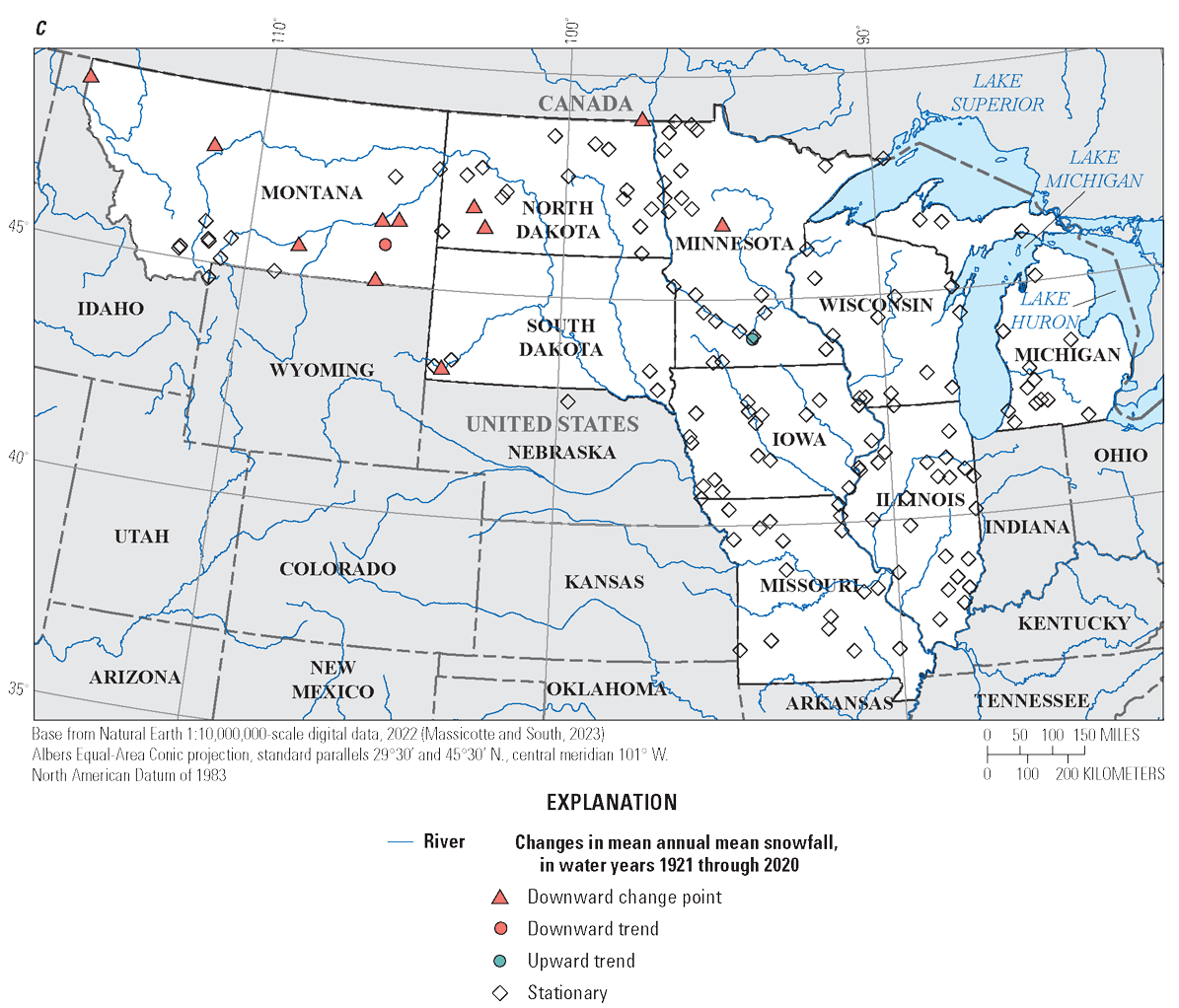
Statistically significant trends and change points for water years 1921 through 2020 at selected U.S. Geological Survey streamgages. A, Annual precipitation. B, Temperature. C, Snow.
Flood Frequency Methods
This section describes the methods used to compute stationary and nonstationary flood frequency estimates in this study. Stationary flood frequency methods used in this report may differ from those outlined in Bulletin 17C (England and others, 2018) and are used here only as a general comparison with nonstationary methods. Nonstationary flood frequency methods can be used to estimate a flood magnitude based on a temporal trend or change point in the peak streamflow (time-adjusted NFFA) or based on an independent variable such as precipitation that is a plausible causal mechanism for the observed peak streamflow nonstationarity (climate-adjusted NFFA). The first part of this section describes methods for estimating nonstationary flood frequency using a regression equation with time as the explanatory variable to model the trend or change point in peak streamflows (Serago and Vogel, 2018). The second part of this section describes methods to compute nonstationary flood probability when the conditional flood distribution is based on a climate variable.
Stationary Flood Frequency
Flood frequency analysis uses statistical techniques to estimate flood magnitudes associated with specific AEPs. An AEP is the probability that a flood of a specific magnitude or higher will occur in a given year. Flood frequency estimates at a streamgage are computed by fitting a probability distribution to the time series of the logarithm of annual peak streamflows. Flood magnitudes for AEPs of interest are computed from the quantiles of the fitted probability distribution. Bulletin 17C recommends fitting a Log-Pearson type III (LP3) distribution for peak streamflow (England and others, 2018). For this study, the method of moments was used to estimate the parameters of the LP3 distribution and corresponding quantiles. This method uses the sample mean (my), standard deviation (sy), and skew (gy) of the logarithms of the peak streamflows (y) to estimate distribution moments, which is shown in equations 1–3. The lmomco package in R (Asquith, 2023) was used to fit the LP3 distributions and compute quantiles from the sample moments.
wheremy
is the sample mean of the log-transformed peak streamflows;
sy
is the sample standard deviation of the log-transformed peak streamflows;
gy
is the sample skew of the log-transformed peak streamflows; and
n
is the number of peak streamflow observations; and
yi
is the natural logarithm of a peak streamflow, in cubic feet per second, for water year i.
The quantity (1+6/n) is a bias correction factor for the skew of an LP3 distribution recommended by Tasker and Stedinger (1986). The stationary FFA method used in this study differs from that recommended by Bulletin 17C, which uses the expected moments algorithm to fit the distribution and also recommends using a weighted or regional skew (England and others, 2018). The method of moments using the sample skew is used here so that comparisons between stationary and nonstationary estimates of flood magnitudes can be made with more consistent methodologies. Bulletin 17C recommends using the multiple Grubbs-Beck test (Cohn and others, 2013) to identify and potentially remove low outlier values to improve the fit of the distribution for the highest streamflows. This method, which assumes stationarity, may not be suitable in NFFA because the thresholds for identifying an outlier may change as the peak streamflow distribution changes through time. Because there is currently no recommended method for identifying or handling outliers in NFFA, and to keep stationary and nonstationary FFA methodologies consistent, all outliers were retained in the dataset.
Conditional Peak Streamflow Moments
When peak streamflows exhibit nonstationarity, the peak streamflow probability distribution changes over time. To estimate a flood AEP for current conditions, the conditional peak streamflow distribution for that year of interest must be determined. Serago and Vogel (2018) introduce expressions for estimating conditional distribution moments derived from a linear regression equation relating nonstationary peak streamflows to an explanatory variable such as a time index, urbanization, or climate variable (eq. 4).
wherey
is the natural logarithm of annual peak streamflows,
ω
is an explanatory variable,
β0, β1
are fitted regression coefficients, and
ε
is a normally distributed error with a mean of zero.
If the regression residuals are homoscedastic and normally distributed, the conditional mean of the peak streamflow distribution can be obtained by solving the regression equation for a specific value of ω (eq. 5).
whereis the conditional mean of y given ω0,
ω0
is the value of the explanatory variable for which the conditional peak distribution is derived, and
β0, β1
are fitted regression coefficients.
The conditional standard deviation can be derived by substituting equation 5 into formulas for standard deviation and skew (eqs. 2 and 3).
whereis the conditional standard deviation of y given ω,
n
is the number of peak streamflow observations,
p
is the number of independent explanatory variables in the regression equation,
yi
is the natural logarithm of peak streamflows, and
is the conditional mean of y given ωi.
The difference is equivalent to the residuals of the fitted regression model and p adjusts for the degrees of freedom in the regression if more than one explanatory variable is used.
There are several derivations for conditional skew based on an OLS regression. Serago and Vogel (2018) and Hecht and others (2022) derive conditional skews based on an OLS regression using time as an explanatory variable. The simplifications made in these derivations apply only to uniformly distributed variables and are not applicable to a stochastic climate variable. This report uses an alternative method of computing the skew introduced in Glas and others (2023), which is applicable for time and climate explanatory variables. This method computes the skew using a standardized time series of peak streamflows:
whereZi
is the standardized peak streamflow,
yi
is the natural logarithm of peak streamflows,
is the conditional mean of y given ωi, and
is the conditional standard deviation of y given ω.
The conditional skew (γZ) can then be computed using Zi instead of yi in equation 3:
wheren
is the number of peak streamflow observations,
Zi
is the standardized peak streamflow,
μZ
is the sample mean of the standardized peak streamflows,
σZ
is the sample standard deviation of the standardized peak streamflows, and
γZ
is the sample skew of the standardized peak streamflows.
Equations 6 and 8 produce a conditional standard deviation and skew that are constants and therefore are most appropriate when the nonstationarity arises from a change in the mean only.
Regression equations used for computing conditional peak streamflow moments should have homoscedastic and normally distributed residuals to avoid biased estimates of conditional moments. Regression residual assumptions were tested using a Breusch-Pagan test of homoscedasticity (Breusch and Pagan, 1979) and a probability plot correlation coefficient (ppcc) test for residual normality (Vogel, 1986). The Breusch-Pagan test was computed using the bptest function in the lmtest package in R (Zeileis and Hothorn, 2002). The null hypothesis for this test is that residuals are homoscedastic. Probability values (p-values) greater than 0.05 indicate an acceptable level of homoscedasticity for regression models. The ppcc test was computed in R using the ppccTest function in the ppcc package (Pohlert, 2020a). This test compares the correlation between the ordered residuals and the theoretical quantiles of a normal distribution. P-values greater than 0.05 and correlations close to 1 indicate that the residuals are likely to be normally distributed.
If the mean and variability of peak streamflows are nonstationary, the regression equation used to model the conditional distribution moments may have heteroscedastic residuals. Hecht and Vogel (2020) developed an approach to estimate the conditional standard deviation (for a regression equation with heteroscedastic residuals. This approach uses a second regression to statistically model the variance of the fitted regression equation (eq. 9), which is then used to determine the conditional variance of the peak streamflow distribution (eq. 10). The residuals, ε, from equation 4 are used as the dependent variable in the variance regression. Equation 9 relates an independent variable to the residuals that have been raised to the 2/3 power. This transformation, called an Anscombe transformation (Anscombe, 1961), produces normally distributed, nonnegative values.
whereεω
are the residuals from a regression equation for peak streamflow (eq. 4),
b0,b1
are fitted regression coefficients,
ω
is an independent variable, and
φ
are normally distributed errors with a mean of zero.
If the residuals of equation 9 are normally distributed and homoscedastic, the conditional variance of peak streamflows (y) given ω0 can be computed according to equation 10 (refer to Hecht and Vogel [2020] for a complete derivation).
whereω0
is the value of the explanatory variable for which the conditional peak distribution is derived,
is the conditional variance of peak streamflows given ω0,
b0,b1
are fitted regression coefficients, and
is the variance of the error terms from the variance regression (eq. 9).
The conditional standard deviation, , in the heteroscedastic case is the square root of equation 10. For this study, the explanatory variable used in equation 10 was assumed to the same as that used in equation 4, although this is not a requirement of the method. If there is evidence that there are different causal mechanisms for the change in mean and the change in variance of peak streamflows, they could be modeled using different explanatory variables (Hecht and Vogel, 2020).
The conditional moments (eqs. 5, 6, 8, 10) can be used to fit a conditional peak flow distribution using the method of moments in the same way as for stationary FFA. Conditional moments can be used to fit any of the common distributions used in FFA. In this study the LP3 distribution is used to maintain consistency with the stationary estimates.
Flood Probability Conditioned on a Stochastic Variable
When the explanatory variable used to model peak streamflows is time, the flood magnitude for a given AEP can be computed directly from the conditional distribution. In this case, the conditional AEP represents the probability that a flood of a given value will occur in year ω0. For example, to update the 1-percent AEP flood estimate to conditions in the year 2020 using a regression equation with water year as the explanatory variable (ω), the conditional mean, standard deviation, and skew could be computed for ω0=2020. Then, the 1-percent AEP could be determined from the quantile of the fitted distribution.
If a climate variable is used as the explanatory variable, ω, in the regression equation (eq. 4), the conditional peak streamflow moments can be computed for a specific value of ω0 using equations 5–10. To estimate the flood frequency for conditions in a specific year of interest, an appropriate value of ω0 is needed for the year of interest. However, because climate variables have random variability from year to year, there is a range of plausible values that ω0 could take in any given year.
For example, annual precipitation and peak streamflow at USGS streamgage 05481000 (Boone River near Webster City, Iowa) have upward trends in peak streamflow and an upward trend in precipitation (fig. 3A, peak streamflow not shown). A conditional flood frequency curve can be generated for peak streamflow for any single value of precipitation using the relation between peak streamflow and precipitation (fig. 3B). When estimating the flood frequency for the year 2020 using equations 5–10, a representative value of precipitation (ω0) is needed. In 2020, the observed annual precipitation was 27.8 inches, the mean annual precipitation estimated by a linear regression is 34.0 inches, and the median annual precipitation estimated by a quantile regression is 35.8 inches. Any of these values may be a plausible value to use for ω0 in equation 5; however, the conditional mean streamflow and the resulting AEP flood magnitude estimate will vary considerably depending on the choice of ω0 (fig. 3A, B).
The conditional probability of a flood for a specific value of annual precipitation is of limited use in most applications because there is a range of possible annual precipitation values that could occur in any given year. Instead, the conditional peak streamflow distribution can be weighted by the probability distribution of annual precipitation for the year of interest to produce a probability-weighted estimate of the flood frequency for the year 2020 (fig. 3C).

Conditional nonstationary flood frequency estimates adjusting for the trend in precipitation obtained from three discrete representative precipitation values for the year 2020 are compared to a distribution-weighted flood frequency estimate for U.S. Geological Survey streamgage 05481000 (Boone River near Webster City, Iowa). A, Mean, median, and observed precipitation for the year 2020 are obtained from annual precipitation data. B, The relation between peak streamflow and precipitation is used to determine the conditional mean peak streamflow for each precipitation estimate. C, Conditional flood frequency curves adjusted for the three precipitation values are compared with a distribution-weighted curve which accounts for the total probability distribution of precipitation for 2020.
The total probability, P(y), of a flood across all probable values of a climate variable can be computed using the law of total probability (Harchol-Balter, 2024).
wherey
is the natural logarithm of a peak streamflow
P(y)
is the probability of y,
P(y|X=)
is the conditional probability of y given a climate variable of magnitude , and
fx()
is the probability density function of the climate variable for a year of interest.
In terms of the NFFA, this law can be generally interpreted as a weighted average of the conditional probability of a flood magnitude (y) given some value of precipitation, weighted by the relative probability of that annual precipitation value, and evaluated across the whole distribution of annual precipitation values.
When obtaining the total probability of a flood of a given magnitude using equation 11, it is necessary to know the probability density of the explanatory variable used to estimate the conditional moments of y. If that distribution is known, the integral can be solved using numerical estimation methods such as quadrature. Quadrature is a method of estimating the area under a curve by dividing into many small rectangular intervals and summing the areas of all the intervals (Chapra and Canale, 2006).
whereP(y)
is the probability of a streamflow of magnitude y;
n
is the number of intervals used;
ωi
is the value of the climate variable for interval i;
is the conditional probability of a flood of magnitude y
fx(ωi)
is the probability density value for a climate variable equal to ωi; and
is the interval width.
Equation 12 computes the probability of a flood with a given magnitude (that is, the probability of a flood of 10,000 cubic feet per second [ft3/s]). Typically, with FFA, the inverse of this function is of interest and the flood magnitude of a given probability is sought (that is, the magnitude of a flood with a 1-percent probability). To estimate the flood magnitude of a specific AEP, optimization can be used to iteratively solve equation 12 across a range of values of y until the AEP of interest is obtained.
When computing the total probability, the conditional probability distribution of the selected climate variable for the year of interest is required. However, assuming the climate variable is the cause of the peak streamflow, nonstationarity means that the climate variable itself is also likely nonstationary, so traditional stationary distribution fitting methods are not applicable to the climate variable of interest. For this study, annual precipitation, temperature, and snow were used as potential explanatory variables for peak streamflow nonstationarity. The conditional distributions for the water year 2020 for climate variables were computed using equations 4–10 with time as the explanatory variable in the regression equation. Lognormal density functions were used for climate variables in equation 12. If future scenarios are of interest, information from large scale climate models could also be used to estimate these climate distributions.
The process used for estimating a flood magnitude for an AEP of interest using a climate-based regression and the law of total probability is outlined below and illustrated in figure 4 using annual precipitation as the climate variable.
-
1. First, a regression equation is developed for log-transformed annual precipitation, ω, using water year as the explanatory variable. The conditional mean and standard deviation of annual precipitation for water year 2020 are computed using equations 5 and 6 (fig. 4A).
-
2. A lognormal conditional probability density function, f(ω), for annual precipitation is fit using the conditional mean and standard deviation from step 1 (fig 4B).
-
3. The probability density curve is divided into n intervals of width . Minimum and maximum values of ω were computed from the 0.0001 and 0.9999 quantiles of the fitted density curve. For each interval, the density function value, fx(ωi), is computed for ωi using the dnorm function in R (fig. 4B).
-
4. A regression equation is developed for log-transformed peak streamflow, y, using log-transformed annual precipitation, ω, as an explanatory variable (fig. 4C). For each value of ωi in step 3, the conditional moments of peak streamflow are determined using equations 5–10 and a conditional LP3 distribution is fit using the method of moments.
-
5. The conditional probability of a flood of magnitude y, , is determined from the fitted conditional distribution in step 4 for each value of ωi (fig. 4D).
-
6. The total probability of a flood of magnitude y is computed from equation 12 using the interval width and probability density of annual precipitation from step 3, and the conditional flood probability from step 5.
-
7. Steps 5 and 6 are repeated across a range of flood magnitudes (y) until step 6 produces the AEP of interest.

Illustration of the steps for estimating the components of equation 13 used for implementing nonstationary flood frequency conditioned on annual precipitation. A, A regression equation relating annual precipitation to water year is used to determine conditional distribution moments for the year 2020. B, The conditional probability density function is evaluated at discrete intervals across the range of the distribution. C, A regression equation relating the logarithm of peak streamflow to the logarithm of annual precipitation is used to determine the conditional moments of the peak streamflow distribution for each interval in part B. D, Conditional flood probability for each precipitation interval is determined by fitting an LP3 distribution to the conditional moments. E, The total probability of a flood of magnitude y is computed by computing the law of probability from the quantities determined in parts B and D.
Confidence Intervals for Flood Frequency Estimates
Bootstrapped 95-percent confidence intervals were computed to assess the uncertainty in stationary FFA and NFFA estimates for the 1-percent AEP flood. For stationary FFA, the peak streamflow data at each streamgage were sampled with replacement for the same length as the period of record. FFA was then performed on the resampled dataset to obtain a bootstrapped estimate. Several different methods of confidence intervals for nonstationary FFA have been developed (Obeysekera and Salas, 2014). In this study, residual bootstrapping of linear regression equations was used to obtain bootstrapped estimates of the conditional mean, standard deviation, and skews for peak streamflow and climate variable distributions (Davison and Hinkley, 1997; Obeysekera and Salas, 2014). The residuals of the fitted linear regression were sampled with replacement and added to the fitted model estimates to create a new bootstrapped dataset. NFFA was then performed on the bootstrapped dataset. For climate-adjusted NFFA, bootstrapping was performed on the linear regression estimating the conditional climate distribution and the linear regression estimating the conditional peak streamflow. For stationary and nonstationary bootstrap methods, confidence intervals were based on 3,000 bootstrapped estimates and computed as the 2.5-percent and 99.5-percent quantiles of the bootstrapped estimates.
Estimation of Flood Frequency at Candidate Streamgages
Prior to using NFFA at a streamgage, peak streamflow nonstationarity should be characterized and if possible, a causal mechanism should be attributed. This is an important step because there are large uncertainties associated with the detection and characterization of nonstationarity in peak streamflows. For example, an apparent trend over a short period of record may actually be a temporary departure from stationary conditions when viewed over a longer period of record, or a change point may be mistakenly characterized as a trend (Lins and Cohn, 2011; Salas and others, 2018). Because of the difficulty in characterizing nonstationarity, exploratory data analysis can help to identify a deterministic, causal mechanism leading to the observed nonstationarity prior to performing NFFA (Koutsoyiannis and Montanari, 2015; Serinaldi and Kilsby, 2015; Slater and others, 2021). Previously published studies have identified changes in precipitation and temperature as likely drivers of changes in peak streamflows in this study area (Levin and Holtschlag, 2022; Sando and others, 2022; Levin, 2024a, 2024b; Marti and Heimann, 2024; Marti and Over, 2024). Additionally, forecasts based on deterministic climate models suggest these trends may continue during the next century (Kunkel and others, 2022). This section describes the process that was used to screen data and apply time- and climate-adjusted NFFA at selected USGS streamgages and provides examples of how regional trend analyses can be used to support NFFA modeling decisions.
Time-Adjusted Nonstationary Flood Frequency
Time-adjusted NFFA uses time as the only explanatory variable to model peak streamflow nonstationarity. This method is computationally simpler than using a stochastic climate variable and does not require additional data; however, it can be difficult to determine the most appropriate model form.
A time series with a change point can display a variety of statistical characteristics. In some cases, a change point may indicate a step change in the mean or variance of the data. In other cases, there may be a change point within a larger gradual trend, or it may indicate a change in direction of a trend slope. Within a linear regression framework there are several approaches that could be used to model a time series with a change point. Using simple linear regression, a step change in the mean can be modeled using an indicator variable that takes the value of 0 for years equal and prior to the change point and 1 after the change point year. The data before and after the change point can be modeled as a constant or changing in time using an additional explanatory variable for time. A change in slope at a change point can be modeled using an interaction term between a change point indicator and a time variable. Other regression methods such as piecewise regression or local linear regression could also be used in situations where there is a nonlinear pattern of nonstationarity (Chen and others, 2010, Bates and others, 2012), but these methods were not tested in this study.
In cases when statistical tests indicate a trend and a change point, it can be difficult to determine the most appropriate regression model form. For example, figure 5 shows peak streamflow for USGS streamgage 05094000 (South Branch Two Rivers at Lake Bronson, Minnesota), which has a statistically significant change point in water year 1961 (p-value<0.001) and trend (p-value=0.001). Using OLS regression, this peak streamflow time series could be modeled using either a trend or a change point. However, predicted flood magnitudes from these two model specifications were very different in a time-adjusted NFFA. In this case, the change point model estimates a conditional mean of 1,949 ft3/s and a 1-percent AEP streamflow magnitude of 5,287 ft3/s for the year 2020, whereas a trend model estimates a conditional mean of 2,885 ft3/s and a 1-percent AEP streamflow magnitude of 9,462.

Annual peak streamflow for U.S. Geological Survey streamgage 05094000 (South Branch Two Rivers at Lake Bronson, Minnesota) for water years 1929 through 2020 modeled with a trend and a change point.
Because trend tests can be affected by the presence of change points, it is generally recommended that change points be identified first and that trend tests are performed separately on subsets of the data before and after the change point (Villarini and others, 2009). Site specific exploratory data analysis of hydroclimatic, land use change, and regulation information, as well as regional nonstationarity analyses such as those found in Marti and others (2024), can be used to support the choice of the regression equation form in cases where nonstationarity test results are ambiguous. Examples 1 and 2, discussed in the upcoming sections, demonstrate time-adjusted NFFA at USGS streamgages with a trend and change point in peak streamflows, respectively. For both examples, climate and streamflow data and analyses in Marti and others (2024) were used to characterize the hydroclimate regime and identify probable causal mechanisms for the peak streamflow nonstationarity. Additionally, climate summaries including historical and future scenarios provided by NOAA for each State are used to provide an additional line of evidence to support the use of NFFA (Kunkel and others, 2022).
Example 1
This example estimates the time-adjusted 1-percent AEP flood at USGS streamgage 04108600 (Rabbit River near Hopkins, Michigan) on the western side of the Lower Peninsula of Michigan. This streamgage has 55 peak streamflow observations from water year 1966 through 2020. Mean annual precipitation during the period of record was 37.3 inches and was typically spread throughout the year without a strong seasonal pattern (Marti and others, 2024). Soil is typically near or at saturated conditions during winter and spring (December through May). Peak streamflows during the period of record occur primarily from December through July, with the highest density of peak streamflows in March and April (Marti and others, 2024).
Upward trends in peak streamflow (p-value=0.02, fig. 6A), annual precipitation (p-value<0.01, fig. 6B), and annual temperature (p-value<0.01, not shown) were identified during the period of record. Seasonal trend analyses in Marti and others (2024) showed upward temperature trends in all seasons, with the largest increases in winter (December through February). Upward trends in precipitation were only in winter (December through February) and spring (March through May). Regional analyses using multiple lines of evidence indicate that increases in spring precipitation and changes in winter temperature may be altering snowmelt dynamics and are plausible drivers of changing peak streamflow (Levin, 2024a).
Climate data at this streamgage, as well as regional trend analyses (Levin, 2024a) that show similar precipitation-driven trends in Michigan, provide strong evidence that increases in peak streamflow at this streamgage may be driven by changes in regional climate. Additionally, statewide climate assessments from NOAA predict that increases in precipitation are likely to continue in southern Michigan during the next century, which supports the use of NFFA for this streamgage (Frankson and others, 2022).

Upward trends for U.S. Geological Survey streamgage 04108600 (Rabbit River near Hopkins, Michigan) for water years 1966 through 2020. A, Peak streamflow. B, Annual precipitation.
Conditional moments of the peak streamflow distribution were computed using a regression equation relating the natural log of peak streamflow (y) and a water year index (wyi), equal to the water year minus 1920. The fitted regression model was y=6.33+0.026×wyi. Fitted regression coefficients for intercept and slope had p-values of less than 0.001 and 0.01, respectively. The residuals do not show evidence of being heteroscedastic (p-value=0.79) or non-normal (p-value=0.94). The conditional mean for the year 2020 was computed from the regression equation using ωyi=100. Conditional standard deviation and skew were fit using equations 5 and 6, respectively. The 1-percent AEP quantile was estimated with the method of moments using the quape3 function in the lmomco R package (Asquith, 2023). The conditional and stationary moments and fitted 1-percent AEP quantile are shown in table 1, and figure 7 shows a comparison of stationary and nonstationary estimates across the range of AEPs. The nonstationary estimate of the 1-percent AEP flood for 2020 was 18 percent higher than the stationary estimate.

Stationary and nonstationary flood frequency curves for U.S. Geological Survey streamgage 04108600 (Rabbit River near Hopkins, Michigan).
Example 2
USGS streamgage 05051600 (Wild Rice River near Rutland, North Dakota) has 58 peak streamflow observations from water years 1960 through 2020. Precipitation has a seasonal pattern with lower precipitation between November and February and higher precipitation in May through July. Median monthly temperatures are typically below freezing from November through March during when streamflow is very low. Streamflow generally increases in the spring as the snowpack melts and precipitation volumes increase. Peak streamflows occur most frequently in the spring primarily owing to snowmelt but can also occur in the summer from large rainstorms (Marti and others, 2024).
Peak streamflows at this location have a statistically significant change point at water year 1992 (p-value<0.001) and a statistically significant upward trend (p-value=0.002, fig. 8A). Mean peak streamflow increased from 82 ft3/s prior to the change point to 468 ft3/s after the change point, which is a 5.7-fold increase. Annual precipitation at this location also has an upward change point in 1990 (p-value=0.016, fig. 8B) and an upward trend (p-value=0.017). An analysis of the timing of peak streamflows and daily streamflows is shown in figure 9A (Marti and others, 2024). In the mid-1990s, there was an abrupt change in the seasonality of peak streamflows. Although peaks prior to the mid-1990s occurred primarily in the spring, after the mid-1990s there was an increase in peaks in May through August (fig. 9A). Additionally, daily streamflows and lower flows increased abruptly in the mid-1990s (fig. 9B). Modelled annual soil storage data indicate that annual soil storage increased concurrent with the change point in precipitation (fig. 9C). The abrupt increase in precipitation and antecedent soil storage during the summer is a likely driver of the change in seasonality and magnitude of peak streamflows.

Upward trends at U.S. Geological Survey streamgage 05051600 (Wild Rice River near Rutland, North Dakota) for A, peak streamflow and B, annual precipitation.


Abrupt changes in streamflow and soil water storage support the use of a change point model for estimating nonstationary peak flows for U.S. Geological Survey streamgage 05051600 (Wild Rice River, near Rutland North Dakota). A, Peak streamflow timing and magnitude. B, Daily streamflow magnitude for each day of the period of record. C, Annual soil water storage. Data are from Marti and others (2024).
Climate data for this streamgage, as well as regional trend analyses (Ryberg and others, 2024), provide strong evidence that increases in peak streamflow at this streamgage may be caused by changes in regional climate. Additionally, the concurrent change point in precipitation and soil moisture, as well as the apparent abrupt change in peak streamflow seasonality and daily streamflow at the time of the change point, provide strong evidence that peak streamflows in this location have undergone an abrupt shift rather than a gradual trend and that time-adjusted NFFA analyses may be more accurately represented with a change point model.
Peak streamflows were transformed using the natural log (y) and a change point indicator variable (cpind) was computed that was equal to 0 for years 1960 through 1992 and equal to 1 from 1993 to 2020. The period after the change point does not have a statistically significant trend (p-value=0.80) and the regression equation used only the change point indicator as an independent variable. The fitted regression equation was y=4.40+1.74×cpind. Fitted regression coefficients for intercept and change point indicator had p-values of less than 0.001. Residuals from this regression did not show significant heteroscedasticity (p-value=0.062) or non-normality (p-value=0.104). The conditional mean after the change point is estimated by the regression equation as =4.4+1.74×1=6.14. Conditional standard deviation and skew were derived from the fitted regression residuals and standardized time series using equations 6 and 9, respectively. The 1-percent AEP quantile was estimated with the method of moments using the quape3 function in the lmomco R package (Asquith, 2023). The conditional and stationary moments and fitted 1-percent AEP quantile are shown in table 2, and figure 10 shows a comparison of stationary and time-adjusted nonstationary estimates across the range of AEPs.

Stationary and time-adjusted nonstationary flood frequency curves for U.S. Geological Survey streamgage 05051600 (Wild Rice River near Rutland, North Dakota).
Climate-Adjusted Nonstationary Flood Frequency Analysis
Climate-adjusted NFFA uses a climate variable to model the nonstationarity in peak streamflow. This method requires a regression equation relating peak streamflow to the climate variable and the probability distribution of the climate variable for the year of interest. Climate-adjusted NFFA is more computationally complex than time-adjusted NFFA and there may be additional uncertainty from the inclusion of the estimated climate probability distribution.
Regional trend attribution studies have identified large-scale changes in climate as a driver of peak streamflow nonstationarity in the study area (Levin and Holtschlag, 2022; Sando and others, 2022). Changes in precipitation magnitude and timing have been identified as likely causes of increasing peak flows in the upper Midwest (Levin and Holtschlag, 2022; Sando and others, 2022). Decreasing peak flows have been attributed to land use change, groundwater withdrawals, decreases in soil moisture, increased temperature, and decreases in snowpack (Neri and others, 2019; Sando and others, 2022). For this study, only annual precipitation, temperature, and snowfall were considered as explanatory variables for regressions estimating peak streamflow. These variables were chosen because of their wide-scale data availability across the region and because they have been used in previous related publications characterizing nonstationarity in this region (Ryberg, 2024).
Because the conditional variance and skew for NFFA analyses are computed from regression residuals, it is important that fitted regressions have residuals that are homoscedastic and normally distributed. Failure to meet these assumptions may result in biased estimates of these distribution parameters. The assumptions of homoscedasticity and normality were tested with the Breusch-Pagan test for homoscedasticity (Breusch and Pagan, 1979) and the probability plot correlation test (Vogel, 1986), respectively. Time-adjusted conditional distribution moments for climate variables were computed for the year 2020 using equations 5–11. Annual climate variables were fit to lognormal probability distributions. The conditional flood and the conditional climate variable distribution were used in the total probability equation (eq. 12) and optimization was used to determine the streamflow magnitude for the 1-percent AEP flood magnitude.
At some streamgages with change points in peak streamflows, there was a change in the relation between peak streamflow and the explanatory climate variable before and after the change point. This change can happen when a change in temperature or soil moisture modifies the relation between precipitation and streamflow (Woodhouse and others, 2016). For example, a step increase in precipitation can increase soil moisture throughout the year. The change in antecedent soil moisture can cause greater streamflow for a given precipitation event after the change point year. In these cases, a change point indicator variable equal to 0 for observations prior to and including the year of the change point and 1 after the change point can be included in the regression equation between peak streamflow and the climate variable to improve the fitted regression equation (refer to ”Example 4” section).
The following examples demonstrate the process of climate-adjusted NFFA at two streamgages. The examples estimate the 1-percent AEP flood using climate conditions for the year 2020.
Example 3
USGS streamgage 05107500 (Roseau River at Ross, Minn.) has 80 peak streamflow observations from water year 1929 through 2020. This streamgage is located along the northern border of Minnesota and streamflow is strongly influenced by snowmelt. Precipitation has a seasonal pattern with lowest precipitation from November through March and highest precipitation in May through July. Median monthly temperatures are typically below freezing from November through March during which time streamflow is very low. Streamflows increase in the spring as the snowpack melts and precipitation volumes increase (Marti and others, 2024).
Peak streamflows at this location have a marginally significant upward change point at water year 1961 (p-value=0.08) and a statistically significant upward trend (p-value=0.02, fig. 11A). Annual precipitation at this location has an upward change point (p-value=0.007) and an upward trend (p-value=0.002, fig. 11B) driven largely by upward trends in winter and spring (Marti and others, 2024). Temperature at this location also increased and had a statistically significant change point (p-value<0.001) in 1979. Increased precipitation accompanied by warmer temperatures, particularly during the winter, which can cause rain-on-snow events and changes in snowmelt dynamics, are consistent as a causal mechanism for the increase in peak streamflows at this location. Climate data for this streamgage, as well as regional trend analyses (Marti and others, 2024), provide strong evidence that increases in peak streamflow at this streamgage may be caused by changes in regional climate. Statewide climate assessments by NOAA predict that high precipitation rates will continue in this region through this century, supporting the use of NFFA at this streamgage (Runkle and others, 2022).

Upward trends and change points at U.S. Geological Survey streamgage 05107500 (Roseau River at Ross, Minnesota) for A, Peak streamflow and B, Annual precipitation.
Conditional moments for peak streamflows were based on the relation between peak streamflows and annual precipitation (fig. 12). The fitted regression equation between the natural log of peak streamflows (y) and natural log of annual precipitation (w) was y=1.78+1.84×w. Residuals for this regression equation do not show evidence of heteroscedasticity (p-value=0.41) or non-normality (p-value=0.21). Conditional moments for peak streamflow were computed using equations 5–8.

Relation between peak streamflow and annual precipitation at U.S. Geological Survey streamgage 05107500 (Roseau River at Ross, Minnesota).
Conditional moments of annual precipitation for the year 2020 were computed from the regression equation relating the natural logarithm of annual precipitation (w) and a change point indicator (cpind) equal to zero prior to and including water year 1961 and equal to 1 after that: w=2.98+0.14×cpind. Residuals from this equation do not show evidence of heteroscedasticity (p-value=0.41) or non-normality (p-value=0.21). The conditional mean of log-transformed annual precipitation for the year 2020 was 3.12, and the standard deviation was 0.179. The conditional probability density function for the log-transformed annual precipitation for the year 2020 was estimated with the dnorm function in R.
Equation 12 was computed across the range of precipitation values from the 0.0001 to 0.9999 quantiles of the computed conditional precipitation distribution. Optimization of equation 12 was performed in R with the optim() function, starting with an initial flood estimate equal to the minimum observed peak streamflow and iterating until the estimated annual exceedance probability was within 0.0002 of the target AEP value (in this case, 1 percent). Estimates of the 1-percent AEP flood using stationary, time-adjusted NFFA, and climate-adjusted NFFA methods are shown in table 3. The conditional mean is not reported in table 3 for climate-adjusted NFFA because there are a range of conditional means used in equation 12. Plots of the annual exceedance probability across a range of values using stationary, time-adjusted NFFA, and climate-adjusted NFFA methods are shown in figure 13.

Stationary and nonstationary flood frequency curves for U.S. Geological Survey streamgage 05107500 (Roseau River at Ross, Minnesota).
Table 3.
Log-Pearson type III distribution moments and 1-percent annual exceedance probability using stationary, time-adjusted nonstationary, and climate-adjusted nonstationary flood frequency methods for water year 2020 for U.S. Geological Survey streamgage 05107500 (Roseau River at Ross, Minnesota).[--, no data]
Example 4
USGS streamgage 06326500 (Powder River near Locate, Montana) has 78 peak streamflow observations from water year 1938 through 2020. Precipitation has a seasonal pattern with lowest precipitation from November and March and highest precipitation in May and June. Median monthly temperatures are typically below freezing from November through March during which time streamflow is very low. Similar to other northern locations in the study area, peak streamflow at this location is influenced by snowfall and snowmelt, which can persist until May or June (Marti and others, 2024).
Peak streamflow at this location has a downward change point in 1972 (p-value=0.001, fig. 14A). There was no trend or change point in precipitation at this location, but nonstationarity was detected in annual snow and annual mean temperature (fig. 14). Annual mean temperature had an upward change point in 1986 (p-value<0.001) and annual snowfall had downward change point in 1979 (p-value=0.02). Previous studies have attributed downward trends in peak streamflow in Montana to combination of precipitation and temperature effects that are difficult to separate (Sando and others, 2022). Nonstationarity in temperature can modify the relation between streamflow and precipitation or snowfall by changing evapotranspiration, soil moisture, and snowmelt processes (Woodhouse and others, 2016). A decrease in snowfall is a likely driver of downward changes in peak streamflow; however, an apparent change in the relation between peak streamflow and snowfall before and after the change point is likely due to the change in temperature (fig. 15).


Change points in streamflow and climate time series at U.S. Geological Survey streamgage 06326500 (Powder River near Locate, Montana). A, Annual peak streamflow. B, Annual snowfall. C, Annual mean temperature.

The relation between the natural log of peak streamflow and the natural log of annual snowfall before and after a change point in 1972.
Conditional moments for peak streamflow were based on the relation among log transformed peak streamflow (y), annual snowfall (w), and a change point indicator variable (cpind) equal to 0 prior to and including the change point year and equal to 1 after (fig. 15). The fitted regression equation was y=7.35+1.74×w–0.56×cpind. All fitted coefficients were statistically significant with p-values<0.01. Residuals for this equation did not show significant heteroscedasticity (p-value=0.54) or non-normality (p-value=0.18). Conditional moments were computed using equations 5–8 (table 4).
Conditional moments for annual snowfall were computed for the year 2020 using the relation between the natural logarithm of annual snowfall (w) and time, using a change point indicator (cpind) equal to zero prior to or equal to 1979 and 1 afterwards, with the equation w=1.11–0.16×cpind. The conditional mean of log-transformed annual snowfall for the year 2020 of 0.95, and the standard deviation was 0.228. The conditional probability density function for the log-transformed annual snowfall for the year 2020 was estimated with the dnorm function in R. Equation 12 was computed across the range of snowfall distribution. Optimization of equation 12 was performed in R with the optim() function, starting with an initial flood estimate equal to the minimum observed peak streamflow and iterating until the estimated annual exceedance probability was within 0.0002 of the target AEP value (in this case, 1 percent).
Estimates of the 1-percent AEP flood using stationary, time-adjusted NFFA, and snowfall-adjusted NFFA methods are shown in table 4. The conditional mean is not reported for climate-adjusted NFFA because there is a range of conditional means used in equation 12. Plots of the annual exceedance probability across a range of values using stationary, time-adjusted NFFA, and climate-adjusted NFFA methods are shown in figure 16. In this case, time-adjusted and climate-adjusted methods produce similar results, both of which estimate lower flood magnitudes than the stationary method.

Stationary and nonstationary flood frequency curves for U.S. Geological Survey streamgage 06326500 (Powder River near Locate, Montana).
Table 4.
Log-Pearson type III distribution moments and 1-percent annual exceedance probability using stationary, time-adjusted nonstationary, and climate-adjusted nonstationary flood frequency methods for water year 2020 for U.S. Geological Survey streamgage 06326500 (Powder River near Locate, Montana).[--, no data]
Regional Applicability of Using Linear Regression in Nonstationary Flood Frequency
Regional assessments of nonstationary flood frequency can benefit from a consistent, broadly applicable method to facilitate comparisons between streamgages or to regionalize the results for prediction at ungaged locations. One goal of the project was to determine whether or not the assumptions of the method could be met across the study area and to identify potential barriers to its usage. Time-adjusted NFFA and climate-adjusted NFFA were attempted at all candidate streamgages in the study area to determine the applicability of this method.
Fitted NFFA models at each site were screened to determine whether the assumptions of homoscedastic, normally distributed residuals were met. Regression equations for which p-values of residuals tests were greater than 0.05 were considered to satisfy OLS regression assumptions and are good candidates for using linear regression for NFFA. Regression equations for which the Breusch-Pagan test for homoscedasticity was less than 0.05 but greater than 0.03 were considered marginally acceptable. Regression equations for which the ppcc test p-value was less than 0.05 but the correlation between residuals and theoretical quantiles of a normal distribution were equal to or greater than 0.98 were also considered marginally acceptable. In these cases, the regression equations may have been affected by one or more outliers or there may be a slight lack of linearity. Marginally acceptable regressions may have greater uncertainty or slight bias but still likely represent the current flood risk better than a stationary estimate. Additional research can help to determine how non-normal residuals or heteroscedasticity in the regression equations affects NFFA estimates. Although not included in this study, the marginal or poor regression fits may potentially be improved using weighted, robust, or multiple linear regression methods; other data transformations; different explanatory variables; or removal of outliers that are not representative of typical peak streamflows. NFFA analyses were not performed for streamgages whose regression equations had p-values below 0.01 in one or both residual tests. The regressions at these streamgages exhibit substantial heteroscedasticity or lack of linearity that may require different explanatory variables or a more flexible statistical framework to adequately estimate conditional moments (Rigby and Stasinopoulos, 2005; Villarini and others, 2009).
Regional Time-Adjusted Nonstationary Flood Frequency Analyses
NFFA using time as the explanatory variable was performed at candidate streamgages in the study area. There were 107 streamgages that had statistically significant change points as well as significant trends, similar to example 2. It was beyond the scope of this study to do detailed site-specific data analyses at all of these streamgages to determine which model form would be more appropriate. Instead, if a change point and trend were identified at a location, it was modeled as a change point as is suggested by Villarini and others (2009).
The model form (change point or trend) of the regression equation used for time-adjusted NFFA and how well the regression residuals met the assumptions of OLS regression are shown in figure 17. Of the 153 candidate streamgages, 103 were modeled with a change point indicator model and 34 were modeled as trends. There were 16 streamgages for which time-adjusted NFFA was not performed because fitted regression residuals exhibited extensive heteroscedasticity or non-normality. Of the 137 streamgages for which time-adjusted NFFA was performed, regression models at 101 streamgages had residuals that did not show significant heteroscedasticity or non-normality or whose residuals could be adequately modeled using a secondary error model (eq. 10), making them good candidates for this NFFA method (fig. 17). The other 36 streamgages had regression equations for which the regression assumptions were marginally met.

Model form and goodness of fit of regression equations used for time-adjusted nonstationary flood frequency at selected U.S. Geological Survey streamgages.
The percent difference in the stationary and time-adjusted nonstationary 1-percent AEP flood estimate was examined at candidate streamgages in the study area (fig. 18). Comparisons of FFA and NFFA methods in this report should be taken only as a screening-level analysis to give an indication of the general magnitude of change. Because it was outside the scope of this study to use the expected moments algorithm (EMA) method of FFA as recommended by Bulletin 17C, the stationary FFA methods used in this study may not match currently published estimates. Despite these limitations, these comparisons give a general estimate of the change in flood magnitudes owing to nonstationarity and may identify regional patterns.

Percent difference between time-adjusted nonstationary flood frequency and stationary flood frequency estimates of the 1-percent annual exceedance probability flood at selected U.S. Geological Survey streamgages.
Differences in flood estimates from time-adjusted NFFA and stationary FFA across the region ranged from −80 percent to 100 percent. The greatest percent differences between stationary FFA and time-adjusted NFFA estimates for the 1-percent AEP flood magnitude were in the northern part of the study area. Upward changes were greatest in eastern North Dakota and Minnesota, whereas the greatest downward changes in estimates were in western North Dakota, South Dakota, and eastern Montana (fig. 18). Differences in the 1-percent AEP were less than 20 percent at most streamgages in Missouri, Michigan, and Illinois.
Time-adjusted NFFA using linear regression was applicable throughout most of the study area. The assumptions of linear regression were adequately met for trend and change point models at most streamgages. Although most streamgages were fit with change point models, nearly all the streamgages with change points also had statistically significant trends. In some cases, site-specific exploratory analysis at individual streamgages (examples 1–4) may lend support for different modeling forms than those selected in this report.
Regional Climate-Adjusted Nonstationary Flood Frequency
Climate-adjusted NFFA was performed at streamgages with a nonstationary annual climate variable that exhibited a statistically significant trend or change point at the 95-percent confidence level that was consistent with the direction of significant change in the peak streamflows (fig. 2). The climate variable selected for use in NFFA at streamgages across the study area is shown in figure 19. Regression equations for upward trends and change points in peak streamflow at streamgages throughout the central part of the study area were fit using annual precipitation if a concurrent upward trend or change point was identified. Regression equations for downward peak streamflow trends and change points in the western part of the study area and in Wisconsin and upper Michigan were fit using either annual temperature or annual snowfall. If temperature and snowfall were nonstationary at a streamgage, the variable with the greater regression coefficient of determination (R2) was chosen. The R2 measures the proportion of the variability in peak streamflow that is explained by the explanatory variable (annual temperature or snowfall). Of the 153 candidate streamgages, 70 were predicted using annual precipitation, 21 were predicted using annual mean temperature, and 7 were predicted using annual snowfall. There were 55 streamgages for which a climate variable could not be identified as a causal mechanism for peak streamflow under the criteria used in this project.

Climate variables used for nonstationary flood frequency at selected U.S. Geological Survey streamgages.
Of the 98 streamgages for which an appropriate climate variable was identified, 65 had fitted regression models with residuals that did not show significant heteroscedasticity or non-normality or whose residuals could be adequately modeled using a secondary error model (eq. 10), making them good candidates for this NFFA method. An additional 33 streamgages had regression equations for which the regression assumptions were marginally met. Climate-adjusted NFFA analyses at these streamgages can benefit from closer examination and may need different explanatory climate variables, a more robust model form, or an alternative NFFA method.
The percent difference between stationary and climate-adjusted NFFA estimates of the 1-percent AEP flood is shown in figure 20. Results were similar to those from the time-adjusted analyses, with the greatest upward changes in eastern North and South Dakota and Minnesota. A comparison of climate and time-adjusted NFFA estimates at streamgages where both analyses were performed is shown in figure 21. Differences between climate- and time-adjusted estimates agreed within 25 percent of each other in about 75 percent of the cases.

Percent difference between climate-adjusted nonstationary flood frequency and stationary flood frequency estimates of the 1-percent annual exceedance probability flood at selected U.S. Geological Survey streamgages.

Comparison of climate-adjusted and time-adjusted nonstationary flood frequency estimates of the 1-percent annual exceedance probability at selected U.S. Geological Survey streamgages.
Climate analyses were applicable in about 60 percent of the streamgages with observed peak streamflow nonstationarity. Many streamgages were excluded from analysis because none of the three annual climate variables could be identified as a probable cause of nonstationarity, either because they were stationary or because the direction of the climate trend or change point was not consistent with a causal mechanism for the peak streamflow trend or change point. In cases where a climate variable was identified as a likely driver of nonstationarity, the method produced 1-percent AEP estimates that were similar in magnitude to those estimated by time-adjusted NFFA methods. Additionally, regression equations using climate variables generally explained a larger portion of the variance than time-based regression equations, with mean coefficient of determination of 0.34 for climate-based regressions and 0.13 for time-based regression equations.
Uncertainty in FFA is high, even under stationary conditions. Sources of uncertainty in stationary FFA include sampling error, uncertainty in estimated sample moments, and the fit of the selected distribution. Many of the same sources of uncertainty in stationary FFA also apply to NFFA. Additionally, NFFA methods in this study are affected by uncertainty from fitted regression equations. Although a full examination of the controls on uncertainty in regression-based NFFA are beyond the scope of this study, the same factors that affect uncertainty in regression are likely to affect NFFA estimates, including sample size, error variance of the fitted regression, and the presence of outliers or influential data points.
Median lower and upper bootstrapped 95-percent confidence intervals were −28 and +38 percent of the estimated value for stationary FFA, −32 and +43 percent for time-adjusted NFFA, and −26 and +55 percent for climate-adjusted NFFA (fig. 22). At some streamgages, NFFA confidence intervals were excessively large, with upper confidence intervals greater than 400 percent. Large confidence intervals occurred at streamgages with shorter periods of record (less than 70 years), those that had large regression error variance, or several large outliers in the data. In general, bootstrapped confidence intervals were larger at streamgages with shorter periods of record where regression slopes were more sensitive to variability in the bootstrapped data and produced a wider range of conditional means. The coefficient of variability of bootstrapped conditional means was twice as large in streamgages with less than 70 years of record than it was at sites with longer periods of record (coefficient of variability of 2.5 and 1.1, respectively). The large range of conditional means reflects the sensitivity of OLS regression slopes to data variability and outliers, particularly when samples sizes are smaller. Additional research can help characterize the factors affecting uncertainty in NFFA estimates; however, this preliminary examination indicates that regression equations that explain a greater portion of the variability and larger sample sizes may produce flood estimates with less uncertainty.

Lower and upper 95-percent confidence intervals for stationary, time-adjusted, and climate-adjusted estimates of the 1-percent annual exceedance probability flood magnitude.
Limitations
Analyses in this study should be regarded as preliminary and do not supersede other published flood frequency estimates. There are several limitations of analyses performed in this study. Only annual precipitation, snowfall, and temperature were considered as potential explanatory variables in this study. These explanatory variables were chosen because of their availability across the large study area and their previous use in characterization of nonstationarity in the study area (Ryberg, 2024); however, subannual climate variables may be better predictors of flood magnitudes at some locations. Additionally, these three climate variables do not represent the full range of flood-generating mechanisms in the region. Changes in land use from agriculture, urbanization, and tile drainage may also have effects on flood magnitude but were beyond the scope of this study. Additionally, only linear OLS regression was considered for estimating the relation between explanatory variables and peak streamflow. Other regression methods such as piecewise regression, robust regression, or multiple regression, which considers the mutual effects of more than one explanatory variable were not considered but may result in better model fits and reduce the uncertainty in estimates. Finally, site-specific exploratory data analyses (examples 1–4) were not completed for the regional application of the method. These regional analyses were performed as a preliminary assessment of the applicability of the method and to identify areas where changes were greatest in the estimated 1-percent AEP. Closer inspection of climate and streamflow trends at individual sites may support the use of different explanatory variables or model forms than those used in this study.
Summary
A primary assumption of flood frequency analysis is that the statistical properties of the peak streamflow time series do not change over time. This assumption has been challenged in recent decades owing to concerns that changes in observed peak streamflows may be caused by changing climate patterns and land-use changes. One approach to nonstationary flood frequency (NFFA) is to model the change in peak streamflows using regression. In this approach, conditional moments for peak streamflow are derived from a regression equation between peak streamflow and an explanatory variable such as time or a climate variable. Flood magnitudes are computed by fitting a probability distribution from the conditional moments and computing the quantiles of the fitted distribution for the annual exceedance probability (AEP) of interest.
For time-adjusted NFFA, the flood magnitude for a given AEP and year is computed directly from the fitted regression equation. For climate-adjusted NFFA, the conditional flood magnitude can be computed for a specific value of the explanatory variable. However, to estimate a climate-adjusted NFFA for a particular year, the probability distribution of the explanatory variable must also be considered. The magnitude for a given AEP flood using a stochastic climate variable can be computed using the law of total probability. This equation integrates the product of the conditional flood frequency and the probability density function of the climate variable. When determining the flood magnitude of an AEP of interest, optimization can be used to iteratively compute the integration until a flood magnitude is that has the selected AEP is determined.
The use of regression in NFFA is appealing owing to its relative ease of application and flexibility to model change points, trends, and some types of nonlinearity through data transformations or other model equations. The use of this method is restricted to situations in which a regression equation can be fit with homoscedastic and normally distributed residuals. Because the conditional moments are derived from the fitted regression and the regression residuals, it is important that the regression assumptions are met. Regression equations with a poor model fit or an incorrect model form (for example, modeling as a trend when the nonstationarity is in fact a change point) can result in greater uncertainty or bias in estimated flood magnitudes.
A nine-State region including Illinois, Iowa, Michigan, Minnesota, Missouri, Montana, North Dakota, South Dakota, and Wisconsin was used as the study area to assess the applicability of ordinary least squares (OLS) regression for NFFA in the study area. Time-adjusted and climate-adjusted NFFA were applied at 153 candidate streamgages with statistically significant peak streamflow trends or change points to determine whether the assumptions of the regressions were met. Regression equations using time as the explanatory variable had residuals that met the OLS assumptions at 101 streamgages and marginally met OLS assumptions at 36 streamgages. Regressions with marginally acceptable residuals exhibited some lack of normality or slight heteroscedasticity, which may result in higher uncertainty but is likely to be a better estimate of flood risk than a stationary model. Time-based regression equations at 16 streamgages exhibited substantial heteroscedasticity or nonstationary patterns, were nonlinear or nonmonotonic, and require more flexible statistical models or other methods of NFFA.
Climate-adjusted NFFA was performed using annual precipitation, annual snowfall, or mean annual temperature as an explanatory variable. Annual precipitation with upward trends or change points was used to estimate 1-percent AEP floods at streamgages with upward trends or change points throughout much of the central parts of the study area. Annual snowfall and temperature had downward trends or change points primarily in the western part of the study area, Wisconsin, and the upper peninsula of Michigan. Annual snowfall or temperature was used to estimate the 1-percent AEP floods at streamgages with downward trends or change points. Of the 153 candidate streamgages, 70 were predicted using annual precipitation, 21 were predicted using annual mean temperature, and 7 were predicted using annual snowfall. There were 55 streamgages for which a climate variable could not be identified as a causal mechanism for peak streamflow under the criteria used in this project or the fitted regression equations exhibited significant heteroscedasticity or non-normality. Regression equations in climate-adjusted NFFA met OLS assumptions at 65 streamgages and marginally met OLS assumptions at 33 streamgages. At streamgages where climate- and time-adjusted NFFA were applied, estimates for 1-percent AEP matched within 25 percent of each other at about 75 percent of the time.
For both NFFA adjustment methods, the difference between stationary and nonstationary NFFA estimates was greatest in the northern part of the region. In areas with upward peak streamflow change points and trends, NFFA estimates were generally less than 20 percent higher than stationary estimates in the southern part of the study area and were greatest in eastern North Dakota and western Minnesota. Wisconsin, Montana, and western South Dakota and North Dakota had primarily downward trends in peak streamflows. Among these areas, eastern Montana and western North Dakota had the largest downward change in the 1-percent estimate from NFFA.
Overall, OLS regression shows promise for large scale application across the study region. Time-adjusted NFFA is somewhat simple to implement and patterns of nonstationarity across most of the region were able to be modeled adequately with OLS regression. OLS regression can be used to adjust flood estimates based on change points or trends in the time series. One challenge in using this method is determining the proper equation form in cases where peak streamflow exhibits a trend and a change point. An incorrect model form can lead to large biases in estimates. Analysis of ancillary climate at the streamgage and regionally can be used to support the choice of model form in these cases. Climate-adjusted NFFA is more computationally complex than time-adjusted NFFA but may be used in cases where a climate attribution of peak streamflow nonstationarity can be confidently made. Climate-based regressions can account for complex patterns of nonstationarity caused by interactions between different climate effects, such as a temperature change point altering the relation between peak flow and precipitation. Climate-based regression equations generally explained a higher portion of the variability in peak streamflows compared to time-based regressions; however, the overall uncertainty in climate-adjusted NFFA estimates may be larger than time-adjusted NFFA estimates owing to the additional uncertainty from the climate distribution probability weighting process. This study used only annual climate variables as potential explanatory variables, but variables on shorter time scales, such as seasonal precipitation, may have better predictive ability in a regression equation.
References Cited
Asquith, W.H., 2023, lmomco—L-moments, censored L-moments, trimmed L-moments, L-comments, and many distributions: R package (version 2.4.9), accessed January 23, 2024, at https://cran.r-project.org/package=lmomco.
Barbhuiya, S., Ramadas, M., and Biswal, S.S., 2023, Nonstationary flood frequency analysis—Review of methods and models, in Pandey, M., Gupta, A.K., and Oliveto, G., eds., River, sediment and hydrological extremes—Causes, impacts and management: Spring, Singapore, p. 271–288. [Also available at https://doi.org/10.1007/978-981-99-4811-6_15.]
Bates, B.C., Chandler, R.E., and Bowman, A.W., 2012, Trend estimation and change point detection in individual climate series using flexible regression methods: Journal of Geophysical Research, v. 117, no. D16, p. 1–9 [Also available at https://doi.org/10.1029/2011JD017077.]
Bracken, C., Holman, K.D., Rajagopalan, B., and Moradkhani, H., 2018, A Bayesian hierarchical approach to multivariate nonstationary hydrologic frequency analysis: Water Resources Research, v. 54, no. 1, p. 243–255. [Also available at https://doi.org/10.1002/2017WR020403.]
Breusch, T.S., and Pagan, A.R., 1979, A simple test for heteroscedasticity and random coefficient variation: Econometrica, v. 47, no. 5, p. 1287–1294 [Also available at https://doi.org/10.2307/1911963.]
Chen, C.W.S., Chan, J.S.K., Gerlach, R., and Hsieh, W.L., 2010, A comparison of estimators for regression models with change points: Statistics and Computing, v. 21, no. 3, p. 395–414 [Also available at https://doi.org/10.1007/s11222-010-9177-0.]
Cohn, T.A., England, J.F., Berenbrock, C.E., Mason, R.R., Stedinger, J.R., and Lamontagne, J.R., 2013, A generalized Grubbs-Beck test statistic for detecting multiple potentially influential low outliers in flood series: Water Resources Research, v. 49, no. 8, p. 5047–5058 [Also available at https://doi.org/10.1002/wrcr.20392.]
Cohn, T.A., and Lins, H.F., 2005, Nature’s style—Naturally trendy: Geophysical Research Letters, v. 32, no. 23, p. 1–5. [Also available at https://doi.org/10.1029/2005GL024476.]
Collins, M.J., Hodgkins, G.A., Archfield, S.A., and Hirsch, R.M., 2022, The occurrence of large floods in the United States in the modern hydroclimate regime—Seasonality, trends, and large-scale climate associations: Water Resources Research, v. 58, no. 2, p. 1–22. [Also available at https://doi.org/10.1029/2021WR030480.]
Davison, A.C., and Hinkley, D.V., 1997, Bootstrap methods and their application: Cambridge University Press, 582 p. [Also available at https://doi.org/10.1017/CBO9780511802843.]
Dewitz, J., and U.S. Geological Survey, 2021, National Land Cover Database (NLCD) 2019 Products (ver. 3.0, February 2024): U.S. Geological Survey data release, accessed January 23, 2024, at https://doi.org/10.5066/P9KZCM54.
Dhakal, N., and Palmer, R.N., 2020, Changing river flood timing in the Northeastern and Upper Midwest United States—Weakening of seasonality over time?: Water (Basel), v. 12, no. 7, p. 1–15. [Also available at https://doi.org/10.3390/w12071951.]
England, J.F., Jr., Cohn, T.A., Faber, B.A., Stedinger, J.R., Thomas, W.O., Jr., Veilleux, A.G., Kiang, J.E., and Mason, R.R., Jr., 2018, Guidelines for determining flood flow frequency—Bulletin 17C (ver. 1.1, May 2019): U.S. Geological Survey Techniques and Methods, book 4, chap. B5, 148 p. [Also available at https://doi.org/10.3133/tm4B5.]
Gilroy, K.L., and McCuen, R.H., 2012, A nonstationary flood frequency analysis method to adjust for future climate change and urbanization: Journal of Hydrology, v. 414–415, p. 40–48 [Also available at https://doi.org/10.1016/j.jhydrol.2011.10.009.]
Glas, R., Hecht, J., Simonson, A., and Gazoorian, C., 2023, Adjusting design floods for urbanization across groundwater-dominated watersheds of Long Island, NY: Journal of Hydrology, v. 618, p. 1–18 [Also available at https://doi.org/10.1016/j.jhydrol.2023.129194.]
Hecht, J.S., Barth, N.A., Ryberg, K.R., and Gregory, A.E., 2022, Simulation experiments comparing nonstationary design-flood adjustments based on observed annual peak flows in the conterminous United States: Journal of Hydrology: X, v. 17, p. 1–24. [Also available at https://doi.org/10.1016/j.hydroa.2021.100115.]
Hecht, J.S., and Vogel, R.M., 2020, Updating urban design floods for changes in central tendency and variability using regression: Advances in Water Resources, v. 136, p. 1–14. [Also available at https://doi.org/10.1016/j.advwatres.2019.103484.]
Hirabayashi, Y., Kanae, S., Emori, S., Oki, T., and Kimoto, M., 2008, Global projections of changing risks of floods and droughts in a changing climate: Hydrological Sciences Journal, v. 53, no. 4, p. 754–772. [Also available at https://doi.org/10.1623/hysj.53.4.754.]
Hodgkins, G.A., Dudley, R.W., Archfield, S.A., and Renard, B., 2019, Effects of climate, regulation and urbanization on historical flood trends in the United States: Journal of Hydrology, v. 573, p. 697–709. [Also available at https://doi.org/10.1016/j.jhydrol.2019.03.102.]
Hodgkins, G.A., Whitfield, P.H., Burn, D.H., Hannaford, J., Renard, B., Stahl, K., Fleig, A.K., Madsen, H., Mediero, L., Korhonen, J., Murphy, C., and Wilson, D., 2017, Climate-driven variability in the occurrence of major floods across North America and Europe: Journal of Hydrology, v. 552, p. 704–717. [Also available at https://doi.org/10.1016/j.jhydrol.2017.07.027.]
Ivancic, T.J., and Shaw, S.B., 2017, Identifying spatial clustering in change points of streamflow across the contiguous U.S. between 1945 and 2009: Geophysical Research Letters, v. 44, no. 5, p. 2445–2453. [Also available at https://doi.org/10.1002/2016GL072444.]
Kendall, M.G., 1938, A new measure of rank correlation: Biometrika, v. 30, no. 1/2, p. 81–93. [Also available at https://doi.org/10.2307/2332226.]
Khaliq, M.N., Ouarda, T.B.M., Ondo, J.C., Gachon, P., and Bobée, B., 2006, Frequency analysis of a sequence of dependent and/or non-stationary hydro-meteorological observations—A review: Journal of Hydrology, v. 329, no. 3–4, p. 534–552. [Also available at https://doi.org/10.1016/j.jhydrol.2006.03.004.]
Koutsoyiannis, D., and Montanari, A., 2015, Negligent killing of scientific concepts—The stationarity case: Hydrological Sciences Journal, v. 60, no. 7–8, p. 1174–1183. [Also available at https://doi.org/10.1080/02626667.2014.959959.]
Kunkel, K.E., Frankson, R., Runkle, J., Champion, S.M., Stevens, L.E., Esterling, D.R., Stewart, B.C., McCarrick, A., and Lemery, C.R., 2022, State climate summaries for the United States 2022: Silver Spring, Maryland, National Oceanic and Atmospheric Administration Technical Report NESDIS 150, accessed January 2025 at https://statesummaries.ncics.org.
Lang, M., Ouarda, T.B.M.J., and Bobeé, B., 1999, Towards operational guidelines for over-threshold modeling: Journal of Hydrology, v. 225, no. 3-4, p. 103–117. [Also available at https://doi.org/10.1016/S0022-1694(99)00167-5.]
Levin, S.B., 2024a, Peak streamflow trends in Michigan and their relation to changes in climate, water years 1921–2020, chap D of Ryberg, K.R., comp., Peak streamflow trends and their relation to changes in climate in Illinois, Iowa, Michigan, Minnesota, Missouri, Montana, North Dakota, South Dakota, and Wisconsin: U.S. Geological Survey Scientific Investigations Report 2023–5064, 49 p., accessed September 2024 at https://doi.org/10.3133/sir20235064D.
Levin, S.B., 2024b, Peak streamflow trends in Wisconsin and their relation to changes in climate, water years 1921–2020, chap. J of Ryberg, K.R., comp., Peak streamflow trends and their relation to changes in climate in Illinois, Iowa, Michigan, Minnesota, Missouri, Montana, North Dakota, South Dakota, and Wisconsin: U.S. Geological Survey Scientific Investigations Report 2023–5064, 49 p., accessed January 2024 at https://doi.org/10.3133/sir20235064J.
Levin, S.B., and Holtschlag, D.J., 2022, Attribution of monotonic trends and change points in peak streamflow in the Midwest region of the United States, 1941–2015 and 1966–2015, chap. D of Ryberg, K.R., ed., Attribution of monotonic trends and change points in peak streamflow across the conterminous United States using a multiple working hypotheses framework, 1941–2015 and 1966–2015: U.S. Geological Survey Professional Paper 1869, p. D1–D22, accessed January 2024 at https://doi.org/10.3133/pp1869.
Lins, H.F., and Cohn, T.A., 2011, Stationarity—Wanted dead or alive?: Journal of the American Water Resources Association, v. 47, no. 3, p. 475–480. [Also available at https://doi.org/10.1111/j.1752-1688.2011.00542.x.]
Mallakpour, I., and Villarini, G., 2015, The changing nature of flooding across the central United States: Nature Climate Change, v. 5, no. 3, p. 250–254. [Also available at https://doi.org/10.1038/nclimate2516.]
Marti, M.K., and Heimann, D.C., 2024, Peak streamflow trends in Missouri and their relation to changes in climate, water years 1921–2020, chap. F of Ryberg, K.R., comp., Peak streamflow trends and their relation to changes in climate in Illinois, Iowa, Michigan, Minnesota, Missouri, Montana, North Dakota, South Dakota, and Wisconsin: U.S. Geological Survey Scientific Investigations Report 2023–5064, 50 p., accessed January 2024 at https://doi.org/10.3133/sir20235064F.
Marti, M.K., and Over, T.M., 2024, Peak streamflow trends in Illinois and their relation to changes in climate, water years 1921–2020, chap. B of Ryberg, K.R., comp., Peak streamflow trends and their relation to changes in climate in Illinois, Iowa, Michigan, Minnesota, Missouri, Montana, North Dakota, South Dakota, and Wisconsin: U.S. Geological Survey Scientific Investigations Report 2023–5064, 58 p., accessed November 2024 at https://doi.org/10.3133/sir20235064B.
Marti, M.K., and Ryberg, K.R., 2023, Method for identification of reservoir regulation within U.S. Geological Survey streamgage basins in the Central United States using a decadal dam impact metric: U.S. Geological Survey Open-File Report 2023–1034, 15 p., accessed January 2024 at https://doi.org/10.3133/ofr20231034.]
Marti, M.K., Wavra, H.N., Over, T.M., Ryberg, K.R., Podzorski, H.L., and Chen, Y.R., 2024, Peak streamflow data, climate data, and results from investigating hydroclimatic trends and climate change effects on peak streamflow in the Central United States, 1921–2020: U.S. Geological Survey data release, accessed April 2024 at https://doi.org/10.5066/P9R71WWZ.
Massicotte, P., and South, A., 2023, rnaturalearth—World map data from Natural Earth: R package version 1.0.1, accessed January 2025 at https://cRAN.R-project.org/package=rnaturalearth.
McCabe, G.J., and Wolock, D.M., 2011, Independent effects of temperature and precipitation on modeled runoff in the conterminous United States: Water Resources Research, v. 47, no. 11, art. W11522, 11 p. [Also available at https://doi.org/10.1029/2011WR010630.]
Millard, S.P., 2013, EnvStats—An R package for environmental statistics: New York, Springer, 307 p. [Also available at https://doi.org/10.1007/978-1-4614-8456-1.]
Milly, P.C.D., Betancourt, J., Falkenmark, M., Hirsch, R.M., Kundzewicz, Z.W., Lettenmaier, D.P., and Stouffer, R.J., 2008, Stationarity is dead—Whither water management?: Science, v. 319, no. 5863, p. 573–574. [Also available at https://doi.org/10.1126/science.1151915.]
Neri, A., Villarini, G., and Napolitano, F., 2020, Statistically-based projected changes in the frequency of flood events across the U.S. Midwest: Journal of Hydrology, v. 584, p. 124314. [Also available at https://doi.org/10.1016/j.jhydrol.2019.124314.]
Neri, A., Villarini, G., Slater, L., and Napolitano, F., 2019, On the statistical attribution of the frequency of flood events across the U.S. Midwest: Advances in Water Resources, v. 127, p. 225–236. [Also available at https://doi.org/10.1016/j.advwatres.2019.03.019.]
Norton, P.A., Delzer, G.C., Valder, J.F., Tatge, W.S., and Ryberg, K.R., 2022, Assessment of streamflow trends in the eastern Dakotas, water years 1960–2019: U.S. Geological Survey Scientific Investigations Report 2022–5055, 11 p., accessed January 2024 at https://doi.org/10.3133/sir20225055.]
Obeysekera, J., and Salas, J.D., 2014, Quantifying the uncertainty of design floods under nonstationary conditions: Journal of Hydrologic Engineering, v. 19, no. 7, p. 1438–1446. [Also available at https://doi.org/10.1061/(ASCE)HE.1943-5584.0000931.]
Ouarda, T.B.M.J., and Charron, C., 2019, Changes in the distribution of hydro-climatic extremes in a non-stationary framework: Scientific Reports, v. 9, no. 8104, p. 1–8 [Also available at https://doi.org/10.1038/s41598-019-44603-7.]
Ouarda, T.B.M.J., and El-Adlouni, S., 2011, Bayesian nonstationary frequency analysis of hydrological variables: Journal of the American Water Resources Association, v. 47, no. 3, p. 496–505 [Also available at https://doi.org/10.1111/j.1752-1688.2011.00544.x.
Over, T.M., Marti, M.K., Ortiz, J., and Podzorski, H.L., 2025, The joint effect of changes in urbanization and climate trends in floods—A comparison of panel and single-station quantile regression approaches: Journal of Hydrology, v. 648, p. 1-21. [Also available at https://doi.org/10.1016/j.jhydrol.2024.132281.]
Over, T.M., Saito, R.J., and Soong, D.T., 2016, Adjusting annual maximum peak discharges at selected stations in northeastern Illinois for changes in land-use conditions: U.S. Geological Survey Scientific Investigations Report 2016–5049, 33 p. [Also available at https://doi.org/10.3133/sir20165049.]
Pettitt, A.N., 1979, A non-parametric approach to the change-point problem: Journal of the Royal Statistical Society—Series C (Applied Statistics), v. 28, no. 2, p. 126–135. [ Also available at https://doi.org/10.2307/2346729.]
Pohlert, T., 2020a, ppcc—Probability Plot Correlation Coefficient test: R package, version 1.2. [Also available at https://CRAN.R-project.org/package=ppcc.]
Pohlert, T., 2020b, trend—Non-parametric trend tests and change-point detection (ver. 1.1.2): Comprehensive R Archive Network (CRAN) digital data, accessed January 2024 at https://CRAN.R-project.org/package=trend.
Rigby, R.A., and Stasinopoulos, D.M., 2005, Generalized additive models for location, scale and shape: Applied Statistics, v. 54, no. 3, p. 507–554. [Also available at https://doi.org/10.1111/j.1467-9876.2005.00510.x.]
Ryberg, K.R., comp., 2024, Peak streamflow trends and their relation to changes in climate in Illinois, Iowa, Michigan, Minnesota, Missouri, Montana, North Dakota, South Dakota, and Wisconsin: U.S. Geological Survey Scientific Investigations Report 2023–5064, [variously paged], accessed November 2024 at https://doi.org/10.3133/sir20235064.
Ryberg, K.R., Akyuz, F.A., Wiche, G.J., and Lin, W., 2016, Changes in seasonality and timing of peak streamflow in snow and semi-arid climates of the north-central United States, 1910–2012: Hydrological Processes, v. 30, no. 8, p. 1208–1218. [Also available at https://doi.org/10.1002/hyp.10693.]
Ryberg, K.R., Hodgkins, G.A., and Dudley, R.W., 2020, Change points in annual peak streamflows—Method comparisons and historical change points in the United States: Journal of Hydrology, v. 583, p. 124307. [Also available at https://doi.org/10.1016/j.jhydrol.2019.124307.]
Ryberg, K.R., Lin, W., and Vecchia, A.V., 2014, Impact of climate variability on runoff in the north-central United States: Journal of Hydrologic Engineering, v. 19, no. 1, p. 148–158. [Also available at https://doi.org/10.1061/(ASCE)HE.1943-5584.0000775.]
Ryberg, K.R., Over, T.M., Levin, S.B., Heimann, D.C., Barth, N.A., Marti, M.K., O’Shea, P.S., Sanocki, C.A., Williams-Sether, T.J., Wavra, H.N., Sando, T.R., Sando, S.K., and Liu, M.S., 2024, Introduction and methods of analysis for peak streamflow trends and their relation to changes in climate in Illinois, Iowa, Michigan, Minnesota, Missouri, Montana, North Dakota, South Dakota, and Wisconsin, chap. A of Ryberg, K.R., comp., Peak streamflow trends and their relation to changes in climate in Illinois, Iowa, Michigan, Minnesota, Missouri, Montana, North Dakota, South Dakota, and Wisconsin: U.S. Geological Survey Scientific Investigations Report 2023–5064, 27 p., accessed January 2025 at https://doi.org/10.3133/sir20235064A.
Salas, J.D., Obeysekera, J., and Vogel, R.M., 2018, Techniques for assessing water infrastructure for nonstationary extreme events—A review: Hydrological Sciences Journal, v. 63, no. 3, p. 325–352. [Also available at https://doi.org/10.1080/02626667.2018.1426858.]
Sando, R., Sando, S.K., Ryberg, K.R., and Chase, K.J., 2022, Attribution of monotonic trends and change points in peak streamflow in the Upper Plains region of the United States, 1941–2015 and 1966–2015, chap. C of Ryberg, K.R., ed., Attribution of monotonic trends and change points in peak streamflow across the conterminous United States using a multiple working hypotheses framework,1941–2015 and 1966–2015: U.S. Geological Survey Professional Paper 1869, p. C1–C36, accessed January 2024 at https://doi.org/10.3133/pp1869.
Serago, J.M., and Vogel, R.M., 2018, Parsimonious nonstationary flood frequency analysis: Advances in Water Resources, v. 112, p. 1–16. [Also available at https://doi.org/10.1016/j.advwatres.2017.11.026.]
Serinaldi, F., and Kilsby, C.G., 2015, Stationarity is undead—Uncertainty dominates the distribution of extremes: Advances in Water Resources, v. 77, p. 17–36. [Also available at https://doi.org/10.1016/j.advwatres.2014.12.013.]
Slater, L.J., Anderson, B., Buechel, M., Dadson, S., Han, S., Harrigan, S., Kelder, T., Kowal, K., Lees, T., Matthews, T., Murphy, C., and Wilby, R.L., 2021, Nonstationary weather and water extremes—A review of methods for their detection, attribution, and management: Hydrology and Earth System Sciences, v. 25, no. 7, p. 3897–3935. [Also available at https://doi.org/10.5194/hess-25-3897-2021.]
Slater, L.J., and Villarini, G., 2016, Recent trends in U.S. flood risk: Geophysical Research Letters, v. 43, no. 24, p. 428–436. [Also available at https://doi.org/10.1002/2016GL071199.]
Tasker, G.D., and Stedinger, J.R., 1986, Regional skew with weighted LS regression: Journal of Water Resources Planning and Management, v. 112, no. 2, p. 225–237. [Also available at https://doi.org/10.1061/(ASCE)0733-9496(1986)112:2(225).]
U.S. Geological Survey [USGS], 2024, USGS water data for the Nation: U.S. Geological Survey National Water Information System database, accessed January 2024 at https://doi.org/10.5066/F7P55KJN.
Villarini, G., Smith, J.A., Baeck, M.L., and Krajewski, W.F., 2011, Examining flood frequency distributions in the Midwest U.S: Journal of the American Water Resources Association, v. 47, no. 3, p. 447–463. [Also available at https://doi.org/10.1111/j.1752-1688.2011.00540.x.]
Villarini, G., Smith, J.A., Serinaldi, F., Bales, J., Bates, P.D., and Krajewski, W.F., 2009, Flood frequency analysis for nonstationary annual peak records in an urban drainage basin: Advances in Water Resources, v. 32, no. 8, p. 1255–1266. [Also available at https://doi.org/10.1016/j.advwatres.2009.05.003.]
Vogel, R.M., 1986, The probability plot correlation coefficient test for the normal, lognormal, and Gumbel distributional hypotheses: Water Resources Research, v. 22, no. 4, p. 587–590. [Also available at https://doi.org/10.1029/WR022i004p00587.]
Vose, R.S., Applequist, S., Squires, M., Durre, I., Menne, M.J., Williams, C.N., Fenimore, C., Gleason, K., and Arndt, D., 2015, Gridded 5km GHCN-daily temperature and precipitation dataset (Nclimgrid) (ver. 1): National Oceanic Atmospheric Administration National Centers for Environmental Information, accessed June 1, 2022, at https://doi.org/10.7289/V5SX6B56.
Wieczorek, M.E., Signell, R.P., McCabe, G.J., and Wolock, D.M., 2022, USGS monthly water balance model inputs and outputs for the conterminous United States, 1895–2020, based on ClimGrid data: U.S. Geological Survey data release, accessed April 26, 2022, at https://doi.org/10.5066/P9JTV1T6.
Woodhouse, C.A., Pederson, G.T., Morino, K., McAfee, S.A., and McCabe, G.J., 2016, Increasing influence of air temperature on upper Colorado River streamflow: Geophysical Research Letters, v. 43, no. 5, p. 2174–2181. [Also available at https://doi.org/10.1002/2015GL067613.]
Zeileis, A., and Hothorn, T., 2002, Diagnostic checking in regression relationships: R News, v. 2, no. 3, p. 7–10. [Also available at https://CRAN.R-project.org/doc/Rnews/.]
Conversion Factors
Temperature in degrees Celsius (°C) may be converted to degrees Fahrenheit (°F) as follows:
°F = (1.8 × °C) + 32.
Temperature in degrees Fahrenheit (°F) may be converted to degrees Celsius (°C) as follows:
°C = (°F – 32) / 1.8.
Supplemental Information
A water year is the 12-month period from October 1 through September 30 of the following year and is designated by the calendar year in which it ends.
Abbreviations
AEP
annual exceedance probability
FFA
flood frequency analysis
LP3
Log-Pearson type III
NAD 83
North American Datum of 1983
NFFA
nonstationary flood frequency analysis
NOAA
National Oceanic and Atmospheric Administration
NWIS
National Water Information System database
OLS
ordinary least squares
ppcc
probability plot correlation coefficient
p-value
probability value
R2
coefficient of determination
USGS
U.S. Geological Survey
For more information about this publication, contact:
Director, USGS Upper Midwest Water Science Center
2280 Woodale Drive
Mounds View, MN 55112
763–783–3100
For additional information, visit: https://www.usgs.gov/centers/umid-water
Publishing support provided by the
Rolla and Reston Publishing Service Centers
Disclaimers
Any use of trade, firm, or product names is for descriptive purposes only and does not imply endorsement by the U.S. Government.
Although this information product, for the most part, is in the public domain, it also may contain copyrighted materials as noted in the text. Permission to reproduce copyrighted items must be secured from the copyright owner.
Suggested Citation
Levin, S.B., 2025, Nonstationary flood frequency analysis using regression in the north-central United States: U.S. Geological Survey Scientific Investigations Report 2025–5034, 33 p., https://doi.org/10.3133/sir20255034.
ISSN: 2328-0328 (online)
Study Area
| Publication type | Report |
|---|---|
| Publication Subtype | USGS Numbered Series |
| Title | Nonstationary flood frequency analysis using regression in the north-central United States |
| Series title | Scientific Investigations Report |
| Series number | 2025-5034 |
| DOI | 10.3133/sir20255034 |
| Publication Date | May 02, 2025 |
| Year Published | 2025 |
| Language | English |
| Publisher | U.S. Geological Survey |
| Publisher location | Reston, VA |
| Contributing office(s) | Upper Midwest Water Science Center |
| Description | Report: viii, 33 p.; Dataset |
| Country | United States |
| State | Illinois, Iowa, Michigan, Minnesota, Missouri, Montana, North Dakota, South Dakota, Wisconsin |
| Online Only (Y/N) | Y |
| Additional Online Files (Y/N) | N |