

Characterization of the Hydrogeologic Framework, Groundwater-Flow System, Geochemistry, and Aquifer Hydraulic Properties of the Shallow Groundwater System in the Wilcox and Lorraine Process Areas of the Wilcox Oil Company Superfund Site Near Bristow, Oklahoma, 2022
Links
- Document: Report (12.7 MB pdf) , HTML , XML
- Data Release: USGS Data Release - Data used for the characterization of the hydrogeologic framework, groundwater-flow system, geochemistry, and aquifer hydraulic conductivity of the shallow groundwater system in the Wilcox and Lorraine process areas of the Wilcox Oil Company Superfund site near Bristow, Oklahoma, 2022
- NGMDB Index Page: National Geologic Map Database Index Page (html)
- Download citation as: RIS | Dublin Core
Acknowledgments
The authors thank the U.S. Environmental Protection Agency remedial project managers, Katrina Higgins-Coltrain (former) and Mark Stead, for providing support in early data compilation, arranging property access for selected data collection efforts, and helping with other aspects of the study. The authors thank Todd Downham of the Oklahoma Department of Environmental Quality for providing information during reconnaissance of the site and for assistance with optimal placement for well installation. The authors also thank Gary Dupert of Environmental Restoration LLC for providing logistical assistance and assisting with site access.
The authors thank their U.S. Geological Survey colleagues Jason Payne and Benjamin Garza for assisting in collection of the geophysical data and Alexandra Adams, Matthew Barnes, and Jason Ramage for assisting in collection of the groundwater geochemical data.
Abstract
The Wilcox Oil Company Superfund site (hereinafter referred to as “the site”) was formerly an oil refinery northeast of Bristow in Creek County, Oklahoma. Historical refinery operations contaminated the soil, surface water, streambed sediments, alluvium, and groundwater with refined and stored products at the site. The Wilcox and Lorraine process areas are where the highest concentrations of volatile organic compounds, semivolatile organic compounds, polycyclic aromatic hydrocarbons, and trace elements (including metals) (collectively hereinafter referred to as “contaminants”) were measured in a local shallow perched groundwater system within the alluvium (hereinafter referred to as the “alluvial aquifer”) at the site during previous site assessments. In order to understand the potential migration of contaminants through the soil and groundwater in these areas, the U.S. Geological Survey, in cooperation with the U.S. Environmental Protection Agency, investigated aquifer characteristics of the alluvial aquifer in the Wilcox and Lorraine process areas of the site to (1) document hydraulic conductivity and other aquifer characteristics of the alluvial aquifer that govern contaminant fate and transport, (2) describe the geospatial extent and concentration of the contaminants in the alluvial aquifer in the Wilcox and Lorraine process areas, and (3) describe the geochemical controls pertaining to oxidation and reduction governing the fate and transport and the degradation potential of contaminants in the groundwater. Various data were compiled and collected to evaluate the aquifer characteristics at the site including the hydrogeologic framework, groundwater-flow system, geochemistry, and hydraulic properties of the aquifer. A total of 20 new (2022) groundwater monitoring wells were installed at the site to collect data used to supplement groundwater-level altitude and groundwater-quality data collected from older, existing groundwater monitoring wells and piezometers. Data compiled and collected for the study were used to evaluate the characteristics of the alluvial aquifer at the site. These aquifer characteristics are defined by the hydrogeologic framework, groundwater-flow system, geochemistry, and hydraulic properties of the aquifer.
Introduction
The Wilcox Oil Company Superfund site (hereinafter referred to as “the site”) was formerly an oil refinery northeast of Bristow in Creek County, Oklahoma (fig. 1). Crude oil was refined and processed at the site from approximately 1915 to 1963 (U.S. Environmental Protection Agency [EPA], 2023a). The Wilcox Oil Refinery began processing oil in the 1920s, after the Lorraine Oil Refinery began processing oil at the site in 1915 (EPA, 2023a). In 1937, the Wilcox Oil Refinery purchased the Lorraine Oil Refinery to expand its operations westward; after the merger the company was renamed the Wilcox Oil and Gas Company (EPA, 2023a). The two process areas where crude oil was refined and processed are hereinafter referred to as the “Wilcox process area” and the “Lorraine process area.” The site contained approximately 80 storage tanks of various sizes, approximately 10 buildings for refinery operations, and various other structures associated with refinery operations, collectively referred to as “historical infrastructure” (fig. 1), as well as contained natural ponds and man-made cooling ponds (EA Engineering, Science, and Technology, Inc., PBC, 2020a, b, c, 2021). Products known to have been refined or stored on site were crude oil, fuel oil, gas oil, distillate, kerosene, naphtha, and benzene (petroleum ether) (EA Engineering, Science, and Technology, Inc., PBC, 2020a, b, c, 2021).
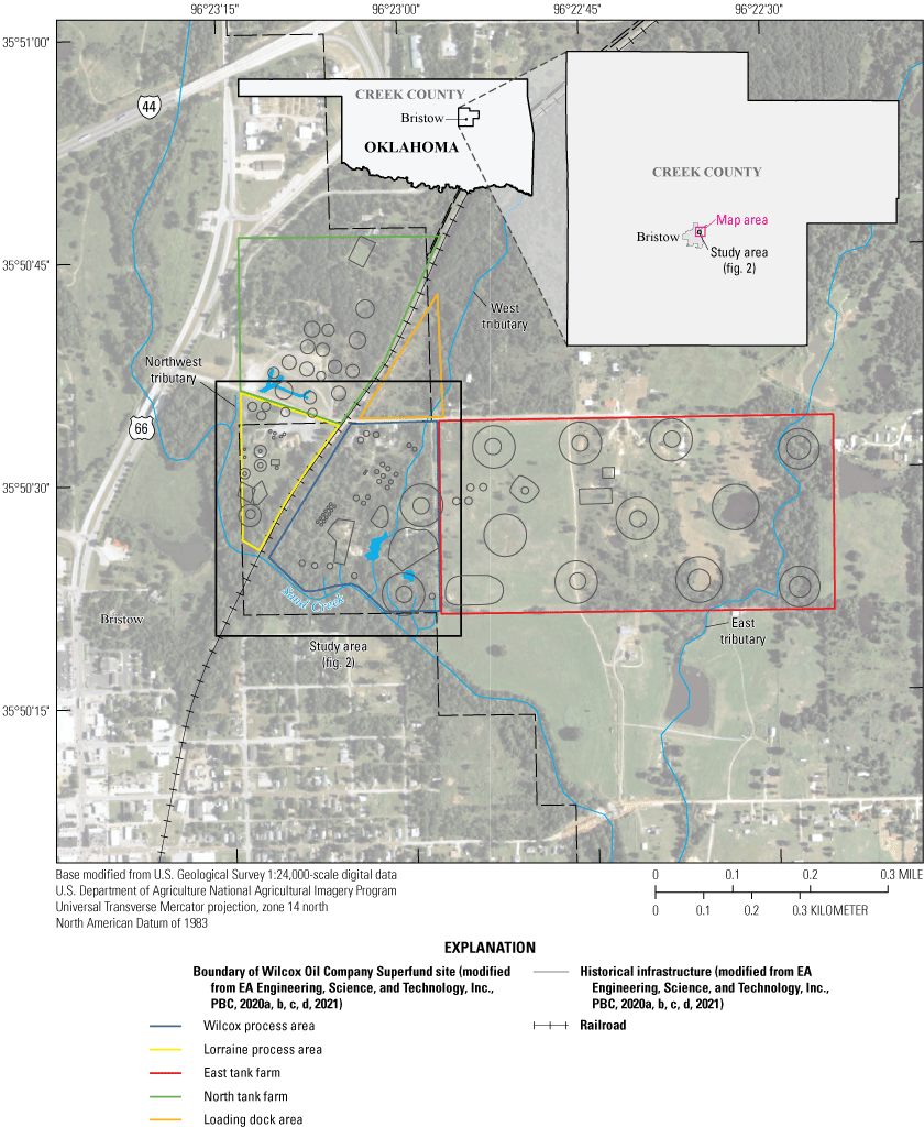
Location of Wilcox Oil Company Superfund site near Bristow, Creek County, Oklahoma.
The Wilcox Oil and Gas Company sold the property in 1963, and most of the equipment and storage tanks were removed by the new property owners, after which the property was sold again to private interests (EA Engineering, Science, and Technology, Inc., PBC, 2020a, b, c, 2021). From 1975 to 2004, the property was parceled out for residential and commercial development, and a church and seven residences were constructed (EA Engineering, Science, and Technology, Inc., PBC, 2020a, b, c, 2021). Although the site was partially cleared during these transitions, remnants of the former oil refining operations and storage tanks remained as of December 2022.
Historical refinery operations contaminated the soil, surface water, streambed sediments, alluvium, and groundwater with refined and stored products at the site (EA Engineering, Science, and Technology, Inc., PBC, 2020a, b, c, 2021; EPA, 2023a). On December 12, 2013, the property formerly owned by the Wilcox Oil and Gas Company was placed on the National Priorities List and was later authorized as a Superfund site when a responsible party for restoration of the site was not identified (EPA, 2023a). As part of the remedial investigation, multiple sampling events have been completed by the Oklahoma Department of Environmental Quality and the EPA. The remedial investigation report (EA Engineering, Science, and Technology, Inc., PBC, 2020a) indicated that subsurface contamination at the site is confined to a shallow perched groundwater system within the alluvium (hereinafter referred to as the “alluvial aquifer”). Approximately 31,000 cubic yards of contaminated soil and 1,349 tons of petroleum waste material have been removed from the site (EPA, 2023a). The alluvial aquifer was susceptible to contamination from the petroleum waste and contaminated soil as a result of precipitation percolating through contaminated soils and alluvium (EA Engineering, Science, and Technology, Inc., PBC, 2021). Groundwater-quality sampling in 2020 indicated that petroleum hydrocarbons were found in the alluvial aquifer at the site but not in the deeper regional groundwater system (EA Engineering, Science, and Technology, Inc., PBC, 2020d, 2021). As indicated in the soil feasibility study report (EA Engineering, Science, and Technology, Inc., PBC, 2021), a data gap analysis (EA Engineering, Science, and Technology, Inc., PBC, 2020d) determined that additional information could help address the areal extent of contamination. The Wilcox and Lorraine process areas are where the highest concentrations of volatile organic compounds (VOCs) (such as benzene), semivolatile organic compounds (SVOCs), polycyclic aromatic hydrocarbons, and trace elements (including metals) (collectively hereinafter referred to as “contaminants”) were measured in the groundwater during previous site assessments. The Wilcox and Lorraine process areas overlie the thickest portions of the alluvium at the site, and understanding the potential migration of contaminants through the soil and groundwater in these areas could help address the areal extent of contamination. Therefore, in 2022, the U.S. Geological Survey (USGS), in cooperation with the EPA, investigated aquifer characteristics of the alluvial aquifer in the Wilcox and Lorraine process areas of the site to help fill data gaps related to the geochemistry, nature and extent of contamination, and the fate and transport and the degradation potential of contaminants in the groundwater.
Purpose and Scope
This report documents the results of a groundwater assessment in the Wilcox and Lorraine process areas of the Wilcox Oil Company Superfund site completed in 2022 by the USGS in cooperation with the EPA. This report builds on the results of previous studies that documented the presence of contaminants in the alluvial aquifer (EA Engineering, Science, and Technology, Inc., PBC, 2020d). This report (1) documents hydraulic conductivity and other aquifer characteristics of the alluvial aquifer that govern contaminant fate and transport, (2) describes the geospatial extent and concentration of the contaminants in the alluvial aquifer in the Wilcox and Lorraine process areas, and (3) describes the geochemical controls pertaining to oxidation and reduction governing the fate and transport and the degradation potential of contaminants in the groundwater.
Description of Study Area
The study area is on the outskirts of Bristow in Creek County, Oklahoma (fig. 1). The site is in a semirural area with about 6,900 people living within 5 miles of its boundaries in 2020 (Center for International Earth Science Information Network [CIESIN] Columbia University, 2023).
The site has a humid subtropical climate, characterized by hot and humid summers and cool to mild winters (Kottek and others, 2006). Climatology data for the city of Bristow compiled by the National Weather Service during 1981–2010 were used to characterize the temperature and precipitation at the site (National Weather Service, 2023). The mean annual temperature is 59.1 degrees Fahrenheit (°F). The coldest month is January, with a mean monthly temperature of 25.8 °F, whereas the warmest month is August, with a mean monthly temperature of 91.5 °F. The mean annual precipitation is 40.98 inches (in.), and the mean annual snowfall is 9.2 in. The wettest and driest months are May and January, with 5.66 and 1.71 in. of mean monthly precipitation, respectively.
The approximately 150-acre site is divided into five major former operational areas: the Wilcox and Lorraine process areas, two main groups of storage tanks that are referred to as the “east tank farm” and “north tank farm,” and the loading dock area (fig. 1) (EPA, 2023a). The focus of this report is on the Wilcox and Lorraine process areas; the other operational areas will not be discussed further in this report. The Wilcox and Lorraine process areas are separated by a railroad that remains in active use (fig. 2). The topography within the Wilcox and Lorraine process areas generally slopes to the south and southwest towards Sand Creek (fig. 2).
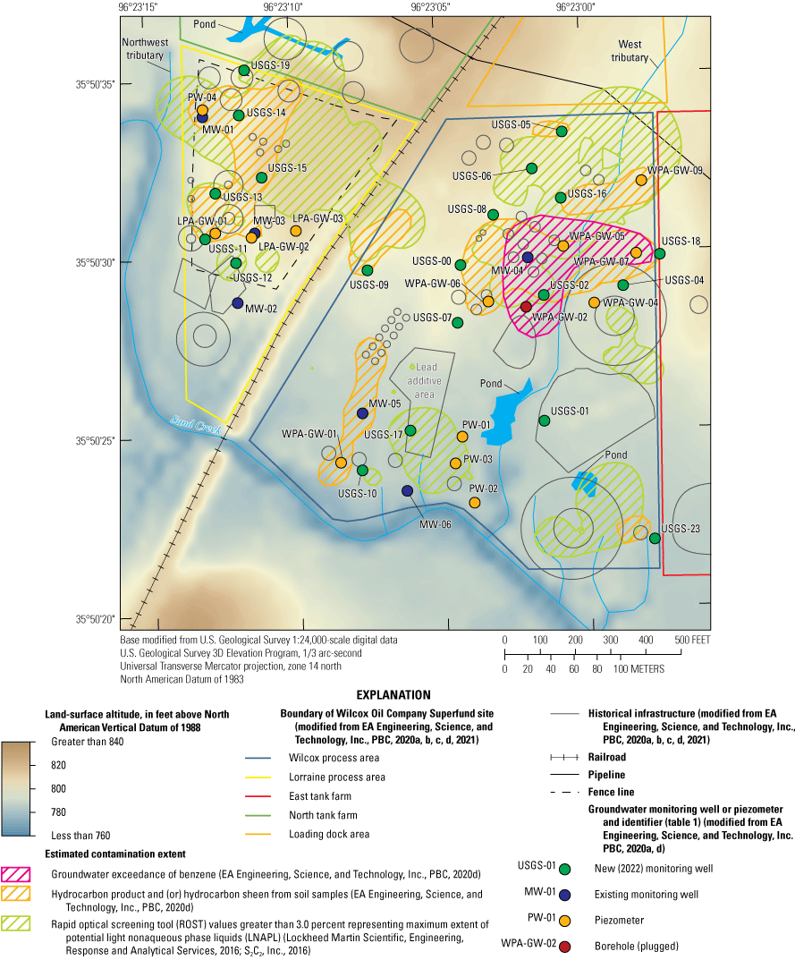
Land-surface altitudes, estimated contamination extents, and groundwater monitoring well or piezometer locations in the Wilcox and Lorraine process areas of the Wilcox Oil Company Superfund site near Bristow, Creek County, Oklahoma.
The Wilcox process area covers approximately 26 acres east of the railroad that divides the site, and most of the infrastructure that existed when the facility was operational has been removed; what remains are dilapidated structures. The location of historical infrastructure associated with the contamination at the site is depicted in figures 1 and 2. Of the infrastructure that remains, there are four aboveground storage tanks, a former lead additive area in the southwestern part of the process area (commonly referred to as “lead sweetening area” [EPA, 2017a]), and two vacant residences that are not delineated on the figures in this report (EA Engineering, Science, and Technology, Inc., PBC, 2020a, b, c, 2021). One of these two vacant residences is in the northern part of the process area and was a former laboratory and office building of the refinery that was later converted into a residence. The second vacant residence is in the eastern part of the process area. Refinery-related debris, such as drums and pieces of scrap iron and piping, was discarded throughout the site (EA Engineering, Science, and Technology, Inc., PBC, 2020a, b, c, 2021). Much of the land surface in the Wilcox process area is barren or shows evidence of plants experiencing unfavorable conditions that hinder their normal growth, development, and metabolism, or stressed vegetation, and petroleum hydrocarbon waste (EA Engineering, Science, and Technology, Inc., PBC, 2020a, b, c, 2021).
The Lorraine process area covers approximately 8 acres west of the railroad (fig. 2), and like the Wilcox process area, most of the infrastructure that existed in the Lorraine process area has been removed. No refinery infrastructure remains in this area, although an abandoned church and a vacant residence still exist (EA Engineering, Science, and Technology, Inc., PBC, 2020a, b, c, 2021). Similar to the Wilcox process area, much of the land surface in the Lorraine process area is barren or shows evidence of stressed vegetation and petroleum hydrocarbon waste (EA Engineering, Science, and Technology, Inc., PBC, 2020a, b, c, 2021).
Perennial and intermittent streams and drainages cross the study area, and contaminants from petroleum hydrocarbon waste have been detected in the surface water and streambed sediments of the streams and ponds (EA Engineering, Science, and Technology, Inc., PBC, 2016, 2020a, b, c, 2021). Sand Creek is a perennial stream south of the Wilcox process area and west and south of the Lorraine process area (fig. 2). An unnamed tributary to Sand Creek referred to hereinafter as the “west tributary” is an intermittent stream that flows southward across the eastern part of the Wilcox process area through a small pond before emptying into Sand Creek (fig. 2). A second unnamed tributary to Sand Creek referred to hereinafter as the “northwest tributary” is an intermittent stream west of the Lorraine process area that flows south before emptying into Sand Creek (fig. 2). Contaminants have mostly been detected in surface-water and streambed-sediment samples from the intermittent west tributary, with few detections in the surface-water and streambed-sediment samples from Sand Creek (surface-water and streambed-sediment samples were not collected from the northwest tributary) (EA Engineering, Science, and Technology, Inc., PBC, 2016, 2020a, b, c, 2021). In addition to the west and northwest tributaries, several other smaller drainages provide flow into Sand Creek during precipitation events within the Wilcox process area, some of which have also been contaminated by historical petroleum hydrocarbon waste as evidenced by the detection of hydrocarbons in soil samples (EA Engineering, Science, and Technology, Inc., PBC, 2016, 2020a, b, c, 2021).
Geologic Setting
The Paleozoic-age (Upper Pennsylvanian Period) Barnsdall Formation of the Ochelata Group is exposed at land surface in parts of the study area (fig. 3). The Barnsdall Formation is composed of two alternating layers of weathering mudstone and two alternating layers of weathering fine-grained quartz arenites (Stanley, 2017). Quartz arenite is a type of sandstone composed of more than 90 percent quartz (Pettijohn and others, 1973). The term “weathering” refers to the breaking down of the mudstone and quartz arenite layers into the silt, clay, and sand particles that compose them as a result of erosional processes.
The total thickness of the Barnsdall Formation in the area around Bristow, Oklahoma, ranges from 50 to 160 feet (ft), and the formation tends to thin to the south (Stanley, 2017). Sandstone outcrops of the Barnsdall Formation (the quartz arenites of the Barnsdall Formation described by Stanley [2017]) are common throughout the site (EA Engineering, Science, and Technology, Inc., PBC, 2020a, 2021). Previous studies (Stanley, 2017; EA Engineering, Science, and Technology, Inc., PBC, 2020a, 2021) indicated that as much as 30 ft of Quaternary-age alluvium overlies the Barnsdall Formation in the Wilcox and Lorraine process areas (fig. 3). The west and northwest tributaries along with Sand Creek likely contributed to the deposition of this alluvium, which consists of sand, silt, clay, and lenticular beds of gravel (EA Engineering, Science, and Technology, Inc., PBC, 2020a, 2021).
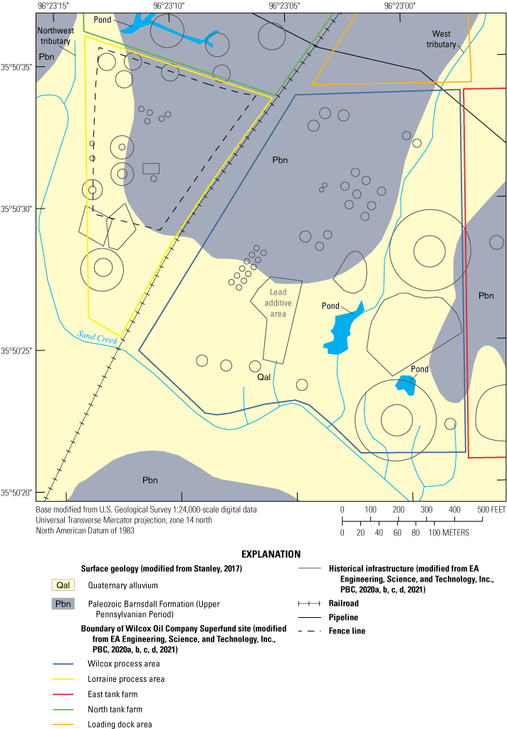
Surface geology in the Wilcox and Lorraine process areas of the Wilcox Oil Company Superfund site near Bristow, Creek County, Oklahoma.
The Natural Resources Conservation Service (NRCS; 2019) identified four main soil classification types associated with the site: Bigheart-Niotaze-Rock outcrop complex, oil-waste land-Huska complex, Ashport silt loam, and Dale clay loam (fig. 4). The Bigheart-Niotaze-Rock outcrop complex soil type is found on slopes ranging from 1 to 8 percent, and the runoff potential increases as the slope increases (NRCS, 2019). The Bigheart soil of the Bigheart-Niotaze-Rock outcrop complex is typically composed of fine sandy loam at depths from land surface of 0–3 in. and of gravelly fine sandy loam at depths from land surface of 3–12 in.; the underlying bedrock extends from 12 to 22 in. below land surface (NRCS, 2019). The Niotaze soil of the Bigheart-Niotaze-Rock outcrop complex is typically composed of fine sandy loam at depths from land surface of 0–16 in. and of silty clay at depths from land surface of 16–40 in. (NRCS, 2019). The Bigheart soil is well drained, whereas the Niotaze soil is poorly drained (NRCS, 2019). The Bigheart-Niotaze-Rock outcrop complex soil type covers the majority of the Lorraine process area, as well as the northern and eastern parts of the Wilcox process area. The oil-waste land-Huska complex is a soil type found in areas contaminated with oil and other liquid waste. Burgess Engineering and Testing, Inc. (2010, p. 2), explained that the “oil-waste land-Huska complex is made up of areas in which liquid oily waste has accumulated. This complex includes slush pits and the adjacent uplands and bottom lands that have been affected by liquid wastes, mainly salt water and oil.” The oil-waste land-Huska complex soil type is moderately well drained and is found on slopes ranging from 1 to 8 percent (NRCS, 2019). The oil-waste land soils of the oil-waste land-Huska complex are found throughout much of the Wilcox process area and consist of loamy and clayey particles weathered from sandstone and mudstone (NRCS, 2019). The Huska soil of the oil-waste land-Huska complex is also found throughout much of the Wilcox process area on slopes ranging from 1 to 8 percent and is typically composed of silt loam at depths from land surface of 0–6 in., silty clay loam at depths from land surface of 6–25 in., and clay at depths from land surface of 25–50 in. The underlying bedrock extends from 50 to 60 in. below land surface (NRCS, 2019). In addition to the oil-waste land-Huska complex soil being found throughout most of the Wilcox process area, it is also found in the eastern part of the Lorraine process area (fig. 4). Both the Ashport silt loam and Dale clay loam soil types occur in floodplains and consist of well-drained particles that provide negligible runoff (NRCS, 2019). The Ashport silt loam soil type is typically composed of silt loam at depths from land surface of 0–48 in. and silty clay loam at depths from land surface of 48–64 in. (NRCS, 2019). The Dale clay loam soil type is typically composed of clay loam at depths from land surface of 0–61 in. (NRCS, 2019) and is found in the southeastern part of the Wilcox process area (fig. 4). The Ashport silt loam soil type is found in the floodplain of Sand Creek in the southern parts of the Wilcox and Lorraine process areas (fig. 4).
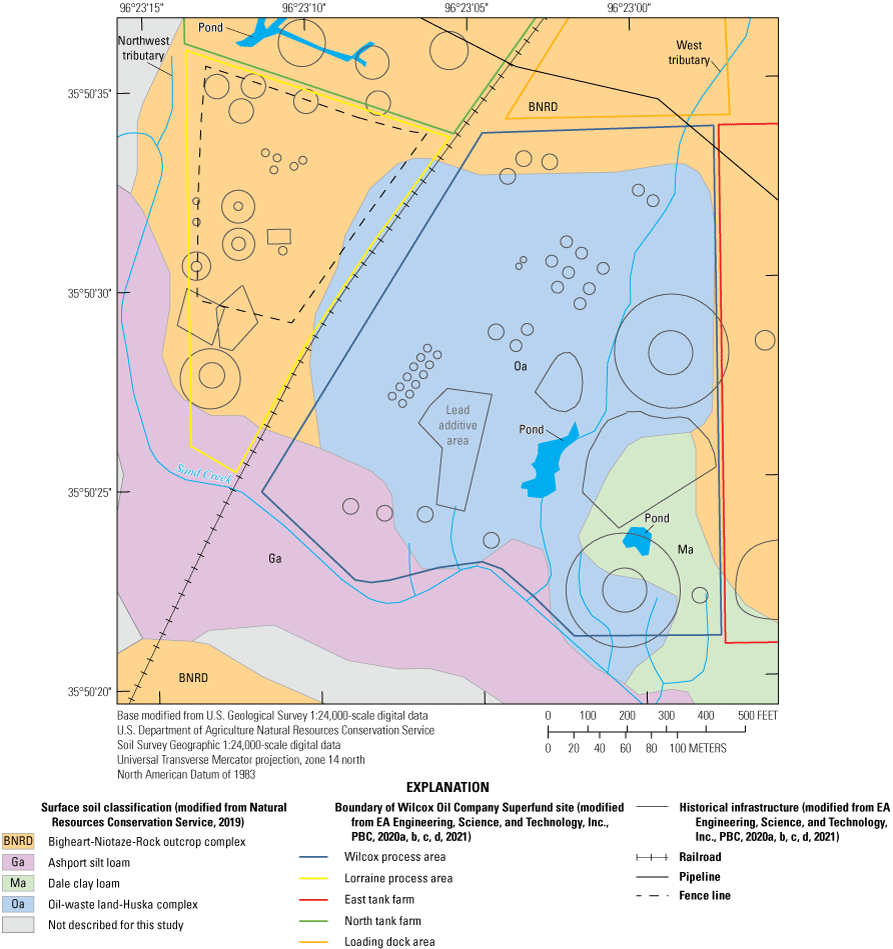
Surface soil classification types in the Wilcox and Lorraine process areas of the Wilcox Oil Company Superfund site near Bristow, Creek County, Oklahoma.
Hydrogeologic Setting
Groundwater at the site is found both in the overlying alluvial aquifer and in the Barnsdall Formation (EA Engineering, Science, and Technology, Inc., PBC, 2020a, 2021). The lower, sand-dominated units of the Barnsdall Formation contain the regional groundwater system (hereinafter referred to as the “bedrock aquifer”), but this bedrock aquifer is not one of the major or minor aquifers identified in Oklahoma by the State of Oklahoma Water Resources Board (Oklahoma Department of Environmental Quality, 1994; Osborn and Hardy, 1999; EA Engineering, Science, and Technology, Inc., PBC, 2020a, 2021). Aquifer characteristics and groundwater quality associated with groundwater contained in the Barnsdall Formation were not assessed as part of this study.
Both the alluvial aquifer and the bedrock aquifer contained in the Barnsdall Formation are generally considered unconfined with the exception that more competent units of the alluvium (where present) might act as lower confining units to the localized alluvial aquifer in some parts of the study area (EA Engineering, Science, and Technology, Inc., PBC, 2020a, 2021). Infiltration of precipitation provides direct recharge to the alluvial aquifer, whereas recharge to the bedrock aquifer occurs through infiltration from precipitation at sandstone outcrops and potentially through downward migration of groundwater from the alluvial aquifer (EA Engineering, Science, and Technology, Inc., PBC, 2020a, 2021). The more competent units of the alluvium acting as a lower confining unit in the eastern part of the Wilcox process area have been truncated by erosion in association with the west tributary and have created conditions favorable for the downward migration of groundwater (EA Engineering, Science, and Technology, Inc., PBC, 2020a, 2021). There is also evidence that the alluvial aquifer discharges to Sand Creek (EA Engineering, Science, and Technology, Inc., PBC, 2020a, 2021).
Groundwater-level altitudes within the alluvial aquifer in the Wilcox and Lorraine process areas generally range from 5 to 16 ft below land surface (EA Engineering, Science, and Technology, Inc., PBC, 2020a, 2021). The bedrock aquifer is slightly deeper than the alluvial aquifer, and groundwater-level altitudes in the bedrock aquifer are likely less than 25 ft below land surface (Oklahoma Department of Environmental Quality, 1994; EA Engineering, Science, and Technology, Inc., PBC, 2020a, 2021). Although few wells at the site were completed in the bedrock aquifer, previous studies (EA Engineering, Science, and Technology, Inc., PBC, 2020a, 2021) indicated that there is not a clear distinction between groundwater-level altitudes in the alluvial aquifer and groundwater-level altitudes in the bedrock aquifer because any local domestic wells at the site were constructed such that the screened interval intercepts both the alluvial aquifer and the bedrock aquifer, facilitating a hydraulic connection between the two aquifers. Groundwater flow within the Wilcox and Lorraine process areas for the alluvial aquifer is generally to the south towards Sand Creek. Based on information shown in figure 3 of EA Engineering, Science, and Technology, Inc., PBC (2020d), the local mean gradient of about 5 ft per 250 ft was indicated for the site, which corresponds to approximately a 0.02 foot per foot (ft/ft) hydraulic gradient. An estimated velocity of 1.3 feet per year (ft/yr) was also reported (EA Engineering, Science, and Technology, Inc., PBC, 2020d).
Previous Studies
The most recent (since 2020) investigation and risk assessment reports that are extensively referenced in this report include the remedial investigation report (EA Engineering, Science, and Technology, Inc., PBC, 2020a), human health risk assessment (EA Engineering, Science, and Technology, Inc., PBC, 2020b), ecological risk assessment (EA Engineering, Science, and Technology, Inc., PBC, 2020c), technical memorandum on data gap investigation (EA Engineering, Science, and Technology, Inc., PBC, 2020d), and soil feasibility study (EA Engineering, Science, and Technology, Inc., PBC, 2021). These reports provided basic information about the site and detailed information on the multiple sampling events and other studies done at the site. The remedial investigation report also identified potential source areas, defined the known contamination extent, and evaluated potential migration pathways.
In 2015, 473 surface soil (less than or equal to a depth of 2 ft below land surface) samples, 355 subsurface soil (greater than a depth of 2 ft below land surface) samples, 44 streambed-sediment samples, 56 surface-water samples, and 35 groundwater samples were collected by EA Engineering, Science, and Technology, Inc., PBC, for the remedial investigation (EA Engineering, Science, and Technology, Inc., PBC, 2020a). These samples, along with 428 surface soil samples collected by the EPA, were used to evaluate the nature and extent of the contamination and to determine potential risks to human health and ecological receptors (EA Engineering, Science, and Technology, Inc., PBC, 2020a). Potential sources that were identified include the skimming and cracking plant, redistillation battery, stills, cooling ponds, lead additive area, tanks, and other historical infrastructure related to refinery activities at the site (figs. 1 and 2) (EA Engineering, Science, and Technology, Inc., PBC, 2020a). Sampling results indicated that the Wilcox process area was the most widely affected area within the site from leaks and spills from the historical refining operations (EA Engineering, Science, and Technology, Inc., PBC, 2020a).
There were 73 surface soil samples collected in the Wilcox process area and 36 surface soil samples collected in the Lorraine process area and analyzed for organic compounds including the polycyclic aromatic hydrocarbons, benzo(a)pyrene, benzene, and ethylbenzene and for metals including lead. Concentrations of benzo(a)pyrene exceeded the residential soil screening value of 0.11 milligram per kilogram (mg/kg) in 35 of the surface soil samples collected in the Wilcox process area and in 7 of the surface soil samples collected in the Lorraine process area (EA Engineering, Science, and Technology, Inc., PBC, 2020a). In the Wilcox process area, benzo(a)pyrene exceedances mainly occurred in samples from the northern and northwestern parts, whereas in the Lorraine process area, benzo(a)pyrene exceedances were mainly in samples from the northwestern and eastern parts. Concentrations of benzene and ethylbenzene exceeded their residential soil screening values of 1.2 and 5.8 mg/kg, respectively, in six of the surface soil samples collected in the Wilcox process area; none of the surface soil samples collected in the Lorraine process area exceeded the benzene and ethylbenzene residential soil screening values (EA Engineering, Science, and Technology, Inc., PBC, 2020a). In the Wilcox process area, benzene and ethylbenzene exceedances mainly occurred in samples from areas near former storage tanks. Concentrations of lead exceeded the residential soil screening value of 400 mg/kg in 19 surface soil samples collected in the Wilcox process area and in 4 surface soil samples collected in the Lorraine process area (EA Engineering, Science, and Technology, Inc., PBC, 2020a). In the Wilcox process area, these lead exceedances were mainly trending southwest from the northeast corner of the area to the area surrounding the former lead additive area, whereas in the Lorraine process area, these lead exceedances occurred mainly near former storage tanks and cooling ponds.
Elevated benzo(a)pyrene concentrations were measured in streambed-sediment samples collected at the site, whereas elevated lead concentrations were measured in both streambed-sediment and surface-water samples collected at the site. Concentrations of benzo(a)pyrene that exceeded the residential soil screening level for this organic compound were most often measured in streambed-sediment samples associated with (1) the west tributary to Sand Creek, (2) the pond fed by the west tributary, (3) the reach of Sand Creek that flows along the southern border of the Wilcox process area, and (4) a downstream location in Sand Creek approximately 700 ft southeast of the site (EA Engineering, Science, and Technology, Inc., PBC, 2020a). Concentrations of lead that exceeded the residential soil screening level for this heavy metal were measured in streambed-sediment and surface-water samples collected from the west tributary to Sand Creek, including the pond fed by the tributary (EA Engineering, Science, and Technology, Inc., PBC, 2020a). The locations where the samples with elevated benzo(a)pyrene and lead concentrations were collected indicate that, although there has been contamination by these constituents in the west tributary to Sand Creek, there likely has not been appreciable contamination to Sand Creek downstream from the Wilcox process area (EA Engineering, Science, and Technology, Inc., PBC, 2020a).
Groundwater sampling results from the remedial investigation indicated that the alluvial aquifer at the site is most likely affected by contamination (EA Engineering, Science, and Technology, Inc., PBC, 2020a). Elevated concentrations of benzene, toluene, and ethylbenzene were measured in the samples collected from well MW-04 (fig. 2), indicating that gasoline distillate is likely present in the groundwater (EA Engineering, Science, and Technology, Inc., PBC, 2020a). The distribution of groundwater exceedances for benzene, toluene, and ethylbenzene at the site indicates that there is a plume of contaminated groundwater near well MW-04 but that the plume has not migrated offsite or into Sand Creek (EA Engineering, Science, and Technology, Inc., PBC, 2020a). However, the remedial investigation report acknowledges that there is a gap in groundwater data and that additional information may help to define the extent of this plume (EA Engineering, Science, and Technology, Inc., PBC, 2020a).
Human health and ecological risk assessments provided information on the distribution of organic compounds and metals that exceeded the human health and ecological screening level criteria at the site. The primary classes of chemicals exceeding those screening levels included VOCs, SVOCs, polycyclic aromatic hydrocarbons, and metals (EA Engineering, Science, and Technology, Inc., PBC, 2020b, c).
In the technical memorandum on data gap investigation (EA Engineering, Science, and Technology, Inc., PBC, 2020d), there was a focus on collecting additional data at existing and at new, temporary wells to further delineate possible contaminant plumes in the Wilcox and Lorraine process areas, gain a better understanding of groundwater and surface-water interactions, and characterize hydraulic and geochemical properties of the alluvial aquifer, including those pertaining to natural attenuation of contaminants. Groundwater-level altitudes measured in existing wells indicated that groundwater flows towards Sand Creek and that the groundwater-level altitude is typically higher than the surface-water altitude in Sand Creek (EA Engineering, Science, and Technology, Inc., PBC, 2020d). Along Sand Creek, groundwater discharges as seepages on the streambank; these seepages are ephemeral and responsive to precipitation, infiltration, recharge, and groundwater movement (EA Engineering, Science, and Technology, Inc., PBC, 2020d). Slug tests were performed by EA Engineering, Science, and Technology, Inc., PBC, at existing wells, and the mean hydraulic conductivity for what they defined as “representative of zones that transmit groundwater at the site” was 0.35 foot per day (ft/d) (EA Engineering, Science, and Technology, Inc., PBC, 2020d, p. 6). Natural attenuation properties for groundwater monitored at the site indicated that elevated iron and manganese concentrations, low oxidation-reduction potential (ORP), and low dissolved oxygen (DO) were present (EA Engineering, Science, and Technology, Inc., PBC, 2020d). The elevated iron and manganese concentrations, low ORP, and low DO indicate that anoxic conditions are present within the aquifer (EA Engineering, Science, and Technology, Inc., PBC, 2020d). The minimal seepage velocity (0.0035 ft/d) of groundwater at the site is supported by these anoxic conditions, including the elevated iron and manganese in groundwater that are in turn oxidized at the point of discharge on the streambanks (EA Engineering, Science, and Technology, Inc., PBC, 2020d).
The groundwater sampling results from the technical memorandum on data gap investigation (EA Engineering, Science, and Technology, Inc., PBC, 2020d) described the predominant contaminants at the site, noteworthy plumes of contaminants in the groundwater, and the remaining potential for aerobic degradation of petroleum hydrocarbons. Benzene was the predominant VOC, exceeding its maximum contaminant level (MCL) of 5.0 micrograms per liter (µg/L) (EPA, 2023b), with a partially defined benzene plume encompassing wells MW-04, WPA-GW-02, WPA-GW-05, and WPA-GW-07 (fig. 2). The only sample with an MCL exceedance for any other SVOCs or polycyclic aromatic hydrocarbons was collected from well WPA-GW-02 with an exceedance of 0.20 µg/L for benzo(a)pyrene (EA Engineering, Science, and Technology, Inc., PBC, 2020d). Two plumes of groundwater contaminated with lead were partially defined, one near the central and northeastern parts of the Wilcox process area and the other near the central part of the Lorraine process area (EA Engineering, Science, and Technology, Inc., PBC, 2020d). There were two plumes of groundwater contaminated with arsenic, one in the Wilcox process area that extended from the southwest to the northwest and the other in the western part of the Lorraine process area (EA Engineering, Science, and Technology, Inc., PBC, 2020d). For the evaluation of sulfate in groundwater at the site, the technical memorandum on data gap investigation (EA Engineering, Science, and Technology, Inc., PBC, 2020d, p. 8) stated, “At MW-04, sulfate has been totally depleted indicating virtually no assimilative capacity for continued sulfate reduction; however, the presence of methane indicates that methanogenesis is ongoing.” The technical memorandum on data gap investigation (EA Engineering, Science, and Technology, Inc., PBC, 2020d) concluded that there was not an appreciable amount of ongoing aerobic degradation of petroleum hydrocarbons.
In 2015, rapid optical screening tool (ROST) measurements were collected in multiple boreholes throughout the site to measure the returning fluorescence from any existing light nonaqueous phase liquids (LNAPLs) that may be present in the subsurface (Lockheed Martin Scientific, Engineering, Response and Analytical Services [Lockheed Martin SERAS], 2016; S2C2, Inc., 2016). The fluorescence from LNAPL contaminants in the subsurface was measured by the ROST as a percentage of relative emittance. The ROST uses a laser to excite hydrocarbon compounds in the subsurface, causing them to fluoresce, and measures the intensity and wavelength distribution of fluorescence emission after excitation (Lockheed Martin SERAS, 2016). A reference oil that provides 100 percent fluorescence was used to calibrate the ROST (Lockheed Martin SERAS, 2016). S2C2, Inc. (2016), used a kriging method to spatially interpolate the fluorescence results and removed fluorescence emittance values if the relative emittance was less than 3 percent. The baseline at the site for fluorescence as a percentage of relative emittance was assumed to be 3 percent (Lockheed Martin SERAS, 2016). According to Lockheed Martin SERAS (2016, p. 13), “This value was chosen based on inspection of the actual ROST logs as well as based on a visual evaluation of kriging results ([that is, less than 3 percent relative emittance], boundary conditions become more apparent which is common in kriged data sets when a given threshold approaches the reporting limit).” Fluorescence values exceeding 3 percent relative emittance are assumed to represent some concentration of LNAPLs in the soil (fig. 2).
The plume of groundwater contaminated with benzene as described in the technical memorandum on data gap investigation (EA Engineering, Science, and Technology, Inc., PBC, 2020d), the extent of the LNAPL concentrations from the ROST dataset (Lockheed Martin SERAS, 2016), and an estimated distribution of sheen or product (EA Engineering, Science, and Technology, Inc., PBC, 2021) were used to aid in the placement of groundwater monitoring wells installed in 2022 at the site for the current study. In this report, the term “groundwater monitoring well” refers to a well where an open hole is drilled, the open hole is installed with well casing and screen interval, the annular space is sealed typically with bentonite grout or pellets, and a surface concrete pad is installed around the well for the main purpose of monitoring groundwater conditions. EA Engineering, Science, and Technology, Inc., PBC (2021), estimated the distribution of petroleum hydrocarbon sheen and (or) hydrocarbon product from temporary monitoring of soil cores and prior assessments of soil samples from the alluvial aquifer in the Wilcox and Lorraine process areas (fig. 2). The soil-core descriptions and depth of refusal data from the ROST cores (S2C2, Inc., 2016) and the soil samples (EA Engineering, Science, and Technology, Inc., PBC, 2020a) were used along with the soil-core descriptions and depth of refusal data from the groundwater monitoring wells installed in 2022 to help characterize the overburden and depth to bedrock at the site. Depth of refusal was defined as the point at which the hammer or other tool used to drill the borehole failed to advance the borehole as additional blows were applied by the tool to the rock being removed (Minnesota Pollution Control Agency, 2023).
An extensive list of other historical documents pertaining to the site follows:
-
• Preliminary assessment of the Wilcox Oil Company (Oklahoma Department of Environmental Quality, 1994),
-
• Expanded site investigation report—Wilcox Oil Company (Roy F. Weston, Inc., 1997),
-
• Site assessment report for Wilcox Refinery (Ecology and Environment, Inc., 1999),
-
• Preliminary assessment of the Lorraine Refinery site (Oklahoma Department of Environmental Quality, 2008),
-
• Site inspection report of the Lorraine Refinery (Oklahoma Department of Environmental Quality, 2009),
-
• Expanded site inspection report, Lorraine Refinery (Oklahoma Department of Environmental Quality, 2010),
-
• Expanded site inspection report, Wilcox Refinery (Oklahoma Department of Environmental Quality, 2011),
-
• Radiation survey, Wilcox Oil Company Superfund site (Oklahoma Department of Environmental Quality, 2016),
-
• Surface-water sampling report, Wilcox Oil Company site (EPA, 2016),
-
• Removal action report for Wilcox Oil Company residence site removal (Weston Solutions, Inc., 2017),
-
• Work plan for investigation of lead contamination at the ethyl blending and lead sweetening areas, Wilcox Oil Company Superfund site (EPA, 2017a),
-
• Source control record of decision summary, Wilcox Oil Company Superfund site (EPA, 2018a), and
-
• Final remedial design report for source control, Wilcox Oil Company Superfund site (EA Engineering, Science, and Technology, Inc., PBC, 2019).
Data Compilation, Collection, and Analysis Methods
Various data were compiled and collected to evaluate the aquifer characteristics at the site including the hydrogeologic framework, groundwater-flow system, geochemistry, and hydraulic properties of the aquifer. A total of 20 new groundwater monitoring wells were installed at the site to collect data used to supplement groundwater-level altitude and groundwater-quality data collected from older, existing groundwater monitoring wells and piezometers. In this report, the term “piezometer” refers to a well that was installed to be a temporary well typically without the annular space being sealed and without a surface concrete pad. Compiled historical soil-core descriptions and depth of refusal information were used in conjunction with collected conductivity logs, soil-core descriptions, and surface geophysical data to characterize the sediments and their extents in the aquifer. Groundwater-level altitude measurements were collected to develop potentiometric-surface maps of the site and to identify potential groundwater-flow direction. Groundwater-quality samples were collected to define the concentration and extent of any contaminants and their byproducts and to estimate natural attenuation potential. An emphasis was placed on understanding the distribution and migration of benzene in the alluvial aquifer because previous studies indicated that it was one of the predominant VOCs in groundwater at the site. Slug tests were completed by the USGS to estimate hydraulic conductivity values at each of the newly installed (2022) groundwater monitoring wells.
Compilation and Review of Historical Data
As mentioned in the “Previous Studies” section of this report, an extensive amount of investigative work has been done at the site, providing an opportunity to compile and review historical data for use in this report. A thorough review of the previously published reports and data was completed to identify pertinent information to aquifer characteristics, such as drillers’ descriptions or previously collected surface or borehole geophysical data and groundwater-quality data. Data were digitized (if not already in digital format) and incorporated into the datasets collected for this study (Teeple and others, 2025). Datasets that were digitized from the previous studies included depth of refusal data from the soil cores done for the remedial investigation (EA Engineering, Science, and Technology, Inc., PBC, 2020a) and the depth of refusal data from the ROST fluorescence logging (S2C2, Inc., 2016). Other data that were not digitized but were used to compare results included soil-core descriptions, maps, and cross sections from the remedial investigation (EA Engineering, Science, and Technology, Inc., PBC, 2020a); soil, streambed-sediment, and water-quality sampling results and maps from the remedial investigation (EA Engineering, Science, and Technology, Inc., PBC, 2020a), technical memorandum on data gap investigation (EA Engineering, Science, and Technology, Inc., PBC, 2020d), and soil feasibility study (EA Engineering, Science, and Technology, Inc., PBC, 2021); and hydraulic conductivity values collected for the technical memorandum on data gap investigation (EA Engineering, Science, and Technology, Inc., PBC, 2020d).
Continuous soil cores were collected for the remedial investigation (EA Engineering, Science, and Technology, Inc., PBC, 2020a) by using direct-push technology (DPT) whereby a machine is used to push sampling tools, instruments, and sensors into the subsurface without the need for a rotary drill to remove the soil (Kejr, Inc., 2023a). Typically, DPT machines rely on static weight and percussive energy to help advance the tool (Kejr, Inc., 2023a). For most of the soil cores at the site using DPT, the soil cores were terminated at the depth of refusal as a result of encountering either well-lithified sandstones or hard, dense clay or mudstone units (EA Engineering, Science, and Technology, Inc., PBC, 2020a). These sandstones or mudstone units are generally related to the sandstones and mudstones of the Barnsdall Formation (Stanley, 2017), and therefore, the depth of refusal is interpreted as the depth to the top of the Barnsdall Formation. Similarly, the ROST fluorescence data were collected by using DPT (S2C2, Inc., 2016). The depths of refusals from the continuous soil cores from the remedial investigation and from the ROST fluorescence logging were compiled and digitized to help interpret the top of bedrock in the Wilcox and Lorraine process areas (Teeple and others, 2025). Land-surface altitudes were determined from a digital elevation model (DEM) for soil-core and ROST fluorescence logging locations by using their horizontal coordinates to provide consistency and improve accuracy. DEM data were obtained from the 3D Elevation Program (3DEP) (USGS, 2017) to estimate land-surface altitudes across the study area.
Existing groundwater monitoring wells and piezometers in the Wilcox and Lorraine process areas were inventoried, and pertinent information (such as location, depth, diameter, screen interval, and water-level and water-quality data) was compiled from wells used in previous studies (fig. 2; table 1) (EA Engineering, Science, and Technology, Inc., PBC, 2020a, b, c, d, 2021). The depth of refusal data from the existing groundwater monitoring wells and piezometers were incorporated into the interpretation for the top of bedrock. These existing groundwater monitoring wells and piezometers were incorporated in the network of groundwater monitoring wells installed for this study, and groundwater-level altitude measurements and groundwater-quality samples were collected in this combined well network; this combined network of wells is hereinafter referred to as “wells.”
Table 1.
Inventory of groundwater monitoring wells and piezometers in the Wilcox and Lorraine process areas of the Wilcox Oil Company Superfund site near Bristow, Creek County, Oklahoma, 2022.[Data from Teeple and others (2025). USGS, U.S. Geological Survey; ID, identifier; ft, foot; NAVD 88, North American Vertical Datum of 1988; bls, below land surface; ─, no data]
| USGS site number | Well ID (fig. 2) |
Latitude, in decimal degrees |
Longitude, in decimal degrees |
Altitude, in ft above NAVD 88 | Type of well | Installed as part of this study? | Depth of refusal, in ft bls | Diameter, in inches | Depth of well, in ft bls | Top of screen, in ft bls | Bottom of screen, in ft bls |
|---|---|---|---|---|---|---|---|---|---|---|---|
| 355034096231301 | MW‑01 | 35.842779 | −96.386949 | 794.3 | Monitoring well | No | ─ | 2.0 | 17.0 | 7.0 | 17.0 |
| 355029096231202 | MW‑02 | 35.841324 | −96.386658 | 793.8 | Monitoring well | No | ─ | 2.0 | 16.0 | 6.0 | 16.0 |
| 355030096231103 | MW‑03 | 35.841863 | −96.386477 | 800.1 | Monitoring well | No | ─ | 2.0 | 12.5 | 7.5 | 12.5 |
| 355029096230104 | MW‑04 | 35.841620 | −96.383870 | 794.1 | Monitoring well | No | ─ | 2.0 | 38.0 | 18.0 | 38.0 |
| 355025096230705 | MW‑05 | 35.840439 | −96.385491 | 786.9 | Monitoring well | No | ─ | 2.0 | 37.0 | 17.0 | 37.0 |
| 355023096230606 | MW‑06 | 35.839826 | −96.385082 | 779.0 | Monitoring well | No | ─ | 2.0 | 50.0 | 30.0 | 50.0 |
| 355024096230401 | PW‑01 | 35.840237 | −96.384541 | 785.6 | Piezometer | No | ─ | 11.0 | 18.0 | ─ | ─ |
| 355023096230401 | PW‑022 | 35.839720 | −96.384440 | 785.3 | Piezometer | No | ─ | 11.0 | 117.0 | ─ | ─ |
| 355023096230403 | PW‑03 | 35.840030 | −96.384613 | 785.3 | Piezometer | No | ─ | 11.0 | 113.5 | ─ | ─ |
| 355034096231304 | PW‑04 | 35.842834 | −96.386946 | 794.0 | Piezometer | No | ─ | 11.0 | 112.0 | ─ | ─ |
| 355030096231201 | LPA‑GW‑01 | 35.841871 | −96.386855 | 796.0 | Piezometer | No | 14.0 | 1.0 | 14.0 | 4.0 | 14.0 |
| 355030096231102 | LPA‑GW‑02 | 35.841830 | −96.386509 | 798.6 | Piezometer | No | 15.0 | 1.0 | 15.0 | 5.0 | 15.0 |
| 355030096230903 | LPA‑GW‑03 | 35.841874 | −96.386083 | 807.4 | Piezometer | No | 15.0 | 1.0 | 15.0 | 5.0 | 15.0 |
| 355024096230801 | WPA‑GW‑01 | 35.840059 | −96.385709 | 784.5 | Piezometer | No | ─ | 1.0 | 25.0 | 15.0 | 25.0 |
| ─ | WPA‑GW‑023 | 35.841235 | −96.383898 | 793.4 | Borehole (plugged)3 | No | ─ | ─ | 24.0 | ─ | ─ |
| 355028096225904 | WPA‑GW‑04 | 35.841254 | −96.383245 | 792.3 | Piezometer | No | 12.0 | 1.0 | 12.0 | 2.0 | 12.0 |
| 355030096230005 | WPA‑GW‑05 | 35.841702 | −96.383527 | 792.5 | Piezometer | No | 22.0 | 1.0 | 22.0 | 12.0 | 22.0 |
| 355028096230306 | WPA‑GW‑06 | 35.841284 | −96.384258 | 793.3 | Piezometer | No | 9.0 | 1.0 | 9.0 | 0.0 | 9.0 |
| 355030096225807 | WPA‑GW‑07 | 35.841634 | −96.382831 | 794.9 | Piezometer | No | 24.0 | 1.0 | 24.0 | 14.0 | 24.0 |
| 355031096225809 | WPA‑GW‑09 | 35.842198 | −96.382763 | 797.4 | Piezometer | No | 15.0 | 1.0 | 15.0 | 5.0 | 15.0 |
| 355029096230400 | USGS‑00 | 35.841574 | −96.384516 | 799.0 | Monitoring well | Yes | 11.0 | 1.5 | 10.0 | 5.0 | 10.0 |
| 355025096230101 | USGS‑01 | 35.840344 | −96.383752 | 788.4 | Monitoring well | Yes | 9.5 | 1.5 | 8.5 | 3.5 | 8.5 |
| 355028096230102 | USGS‑02 | 35.841324 | −96.383726 | 790.9 | Monitoring well | Yes | 7.0 | 1.5 | 6.0 | 1.0 | 6.0 |
| 355029096225804 | USGS‑04 | 35.841384 | −96.382964 | 792.6 | Monitoring well | Yes | ─ | 1.5 | 20.0 | 10.0 | 20.0 |
| 355033096230005 | USGS‑05 | 35.842594 | −96.383513 | 801.5 | Monitoring well | Yes | 9.5 | 1.5 | 9.0 | 4.0 | 9.0 |
| 355032096230106 | USGS‑06 | 35.842312 | −96.383809 | 801.6 | Monitoring well | Yes | 9.5 | 1.5 | 9.0 | 4.0 | 9.0 |
| 355027096230407 | USGS‑07 | 35.841125 | −96.384558 | 796.1 | Monitoring well | Yes | 10.0 | 1.5 | 9.5 | 4.5 | 9.5 |
| 355030096230308 | USGS‑08 | 35.841959 | −96.384190 | 800.4 | Monitoring well | Yes | 15.0 | 1.5 | 15.0 | 5.0 | 15.0 |
| 355029096230709 | USGS‑09 | 35.841552 | −96.385408 | 795.6 | Monitoring well | Yes | 14.0 | 1.5 | 12.5 | 7.5 | 12.5 |
| 355023096230710 | USGS‑10 | 35.839995 | −96.385506 | 785.2 | Monitoring well | Yes | ─ | 1.5 | 20.0 | 10.0 | 20.0 |
| 355030096231311 | USGS‑11 | 35.841827 | −96.386954 | 795.0 | Monitoring well | Yes | 13.0 | 1.5 | 10.0 | 5.0 | 10.0 |
| 355029096231112 | USGS‑12 | 35.841636 | −96.386664 | 795.7 | Monitoring well | Yes | 13.0 | 1.5 | 12.0 | 2.0 | 12.0 |
| 355031096231313 | USGS‑13 | 35.842181 | −96.386845 | 800.5 | Monitoring well | Yes | 11.0 | 1.5 | 10.5 | 5.5 | 10.5 |
| 355033096231114 | USGS‑14 | 35.842786 | −96.386600 | 797.9 | Monitoring well | Yes | 19.0 | 1.5 | 19.0 | 4.0 | 19.0 |
| 355032096231115 | USGS‑15 | 35.842296 | −96.386397 | 807.7 | Monitoring well | Yes | 10.0 | 1.5 | 10.0 | 5.0 | 10.0 |
| 355031096225916 | USGS‑16 | 35.842078 | −96.383539 | 796.2 | Monitoring well | Yes | ─ | 1.5 | 20.0 | 5.0 | 20.0 |
| 355025096230617 | USGS‑17 | 35.840295 | −96.385037 | 787.7 | Monitoring well | Yes | ─ | 1.5 | 20.0 | 10.0 | 20.0 |
| 355029096225718 | USGS‑18 | 35.841621 | −96.382605 | 796.6 | Monitoring well | Yes | 9.0 | 1.5 | 9.0 | 4.0 | 9.0 |
| 355034096231119 | USGS‑19 | 35.843136 | −96.386538 | 802.6 | Monitoring well | Yes | 19.0 | 1.5 | 18.0 | 3.0 | 18.0 |
| 355022096225823 | USGS‑23 | 35.839404 | −96.382724 | 783.9 | Monitoring well | Yes | ─ | 1.5 | 20.0 | 10.0 | 20.0 |
Piezometer was located on site and sampled. Location of well does not directly match with published reports, but there were two piezometers nearby that may correlate with this piezometer: TF-34-DISCH and TF-34-01 (Lockheed Martin Scientific, Engineering, Response and Analytical Services, 2016); TF-34-DISCH is the more likely piezometer.
Groundwater Monitoring Well Installation
Twenty new groundwater monitoring wells were installed at the site by the USGS in October 2022 (fig. 2; table 1) by using a Geoprobe DPT drilling system (Kejr, Inc., 2023b) to collect groundwater-level altitude measurements and groundwater-quality samples within the alluvial aquifer, thus supplementing the existing data from older wells at the site. The new groundwater monitoring wells were all screened in the alluvial aquifer to facilitate future monitoring and sampling efforts and installed to a depth of 20 ft or the depth of refusal, which is explained further in the “Compilation and Review of Historical Data” section of this report. The total depth of 20 ft was selected because the focus of this study was the alluvial aquifer, and the depth to groundwater was typically no more than 15 ft; the intent was to have at least a 5-ft screen interval below the top of the groundwater table. An electrical conductivity (EC) log and a soil core were collected at each location where a groundwater monitoring well was installed to better understand and correlate observations in the subsurface and more accurately determine contamination zones. The borehole EC logs, soil-core descriptions, and well construction information were published in a companion data release to this report (Teeple and others, 2025), and the borehole EC logs were also archived in the USGS GeoLog Locator (USGS, 2024).
Borehole Electrical Conductivity Logging
EC is the relative ability of earth material to transmit a current. As discussed in Teeple (2017, p. 6), “The electrical properties of soil and rock are determined by water content, porosity, clay content, and conductivity (reciprocal of electrical resistivity) of the pore water (Lucius and others, 2007). * * * Electrical changes detected within the subsurface also reflect changes that occur within the hydrogeology.” Prior to installing a groundwater monitoring well at a given location, a borehole EC log was collected using a 1.5-in.-diameter Geoprobe EC sensor (Kejr, Inc., 2023c). The sensor is at the tip of the DPT drive-head device and uses an array of four electrodes (two transmitter [Tx] electrodes and two receiver [Rx] electrodes) to measure EC of the soil in millisiemens per meter as it is pushed into the subsurface (fig. 5A) (Teeple, 2017). A known current was transmitted into the subsurface through the Tx electrodes, and the resulting electrical potential was measured as a voltage change between the two Rx electrodes (Teeple, 2017). Using the known current, the measured voltage values, and the geometric factor dependent on the array, a conductivity value was calculated by using Ohm’s law (fig. 5B) (Teeple, 2017). For this study, EC values were typically lower in coarse-grained sediments such as sand or gravel than in fine-grained sediments such as clay and silt or sediment contaminated with previously refined or stored products at the site. Data were not collected or were unusable because of issues with the EC probe at wells USGS-12, USGS-19, and USGS-23.
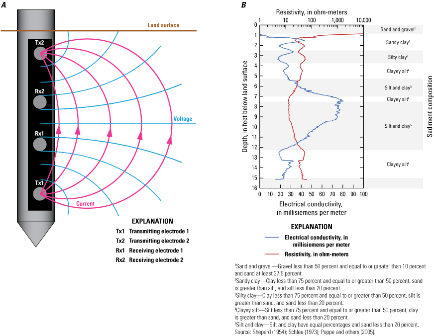
(A) The direct-push electrical conductivity method (modified from Teeple, 2017). (B) Example of the electrical conductivity and resistivity from borehole electrical conductivity logging at the Wilcox Oil Company Superfund site near Bristow, Creek County, Oklahoma, October 2022.
Collecting Soil Cores
Directly adjacent to the EC borehole, a 1.5-in.-diameter soil core was collected to the same depth, if possible. The variability of consolidated sediments resulted in varying depths of penetration even if the tool was moved just a few feet; depths typically varied between the EC borehole and adjacent soil core by about 0.5 to 1 ft, but greater differences sometimes occurred. The soil core was segmented into lithologic units wherein each segment that was discernable from the unit above and below was individually described for color, grain size, and sorting by using field charts based on methods outlined in Wentworth (1922), Shepard (1954), Compton (1962), Schlee (1973), Folk (1980), Munsell Color Co., Inc. (1992), and Poppe and others (2005). The soil-core descriptions were made onsite and then later digitized to a machine-readable text file (Teeple and others, 2025).
A photoionization detector (PID) was used to monitor the presence of VOCs during groundwater monitoring well installation. VOC off-gassing was monitored throughout the drilling and soil-core description processes. The VOC concentration values detected were used to determine the severity of contamination at each location where a groundwater monitoring well was installed at the site. The PID was used only to detect general VOCs, so the presence of specific VOCs was not determined during groundwater monitoring well installation. The VOC concentration and saturation were noted in the soil-core description (Teeple and others, 2025). Once a groundwater monitoring well was installed, the soil core was disposed of properly, as it contained contaminants from the subsurface alluvium.
Groundwater Monitoring Well Completion
After collecting the soil core, the Geoprobe DPT drilling system was used to install the groundwater monitoring well; each groundwater monitoring well was installed by directly pushing a 3.25-in.-outer-diameter rod with an expendable point down the same hole where the soil core was collected. After reaching the desired depth, the prepacked screens (Kejr, Inc., 2023d) and 1.5-in. polyvinyl chloride (PVC) risers were placed inside the 3.25-in. rod, with the screens placed at an optimal depth for groundwater sampling. The prepacked screens were made of slotted PVC wrapped in sand and stainless-steel mesh (Kejr, Inc., 2023d). The outer diameter of the screens was 2.5 in. with an inner diameter of 1.5 in. (Kejr, Inc., 2023d). The prepacked screens were secured in the borehole with 20/40 mesh sand (more than 90 percent of the sand grains by weight are between 0.85 and 0.425 millimeter) (Zheng and Tannant, 2016). Annular sealing was completed by using sodium bentonite pellets (0.25- to 0.75-in. size) starting from about 0.5 ft above the top of the screen to about 2 ft below land surface. The surface seal was completed with concrete from land surface to a depth of about 2 ft below land surface. Well construction information was noted in the field and then later digitized to a machine-readable text file (Teeple and others, 2025). Each groundwater monitoring well was geospatially referenced with coordinates collected from a real-time kinematic (RTK) Global Positioning System (GPS) receiver.
Development of the Top of Bedrock Surface
The depth of refusal from the soil cores for the remedial investigation, the ROST fluorescence logging, and the groundwater monitoring wells installed in 2022 (Teeple and others, 2025) were used to create a top of bedrock surface grid. Depth of refusal data were converted to refusal altitudes by subtracting the depths from the 3DEP DEM. The top of bedrock surface grid was created by using Oasis montaj (Seequent, 2025). A kriging method featuring “trend removal” (elimination of spatial data artifacts) is included in Oasis montaj (Seequent, 2020). There are different variogram parameters and models to choose from in the Oasis montaj software; the default kriging parameters for an exponential variogram model were used (Seequent, 2020). The grid cell size used was a horizontal grid spacing of 5 by 5 meters (m). The top of bedrock grids were iteratively compared to the refusal altitudes to evaluate outliers and grid accuracy and identify clustered data. All outlier locations were evaluated through a correlation process to determine data-point uncertainty. The correlation process involved the comparison of refusal altitudes between the given site and nearby sites. Throughout the process, all refusal altitudes were reviewed and revised as needed to provide the best possible final representation of the top of bedrock.
Surface Geophysical Data Collection
Surface geophysical resistivity methods have been used extensively by Teeple (2017) and Teeple and others (2009a, b, c, 2021) for site characterization and hydrogeologic framework development, and the methods used herein and their detailed descriptions are adapted from those reports, especially when discussing the frequency domain electromagnetic (FDEM) (Teeple and others, 2009c; Teeple, 2017) and electrical resistivity tomography (ERT) (Teeple and others, 2009a, b, c; Teeple, 2017) methods and the integration of geophysical data from multiple methods (Teeple, 2017). Similar to the borehole EC logging done during groundwater monitoring well installation, surface geophysical resistivity methods can be used to detect spatial changes in the electrical properties of the subsurface (Zohdy and others, 1974); electrical changes detected within the subsurface can reflect changes that occur within the hydrogeology. Geophysical methods (which are relatively noninvasive) are therefore valuable for interpreting hydrogeologic characteristics in areas between wells, where typically little to no information is available. FDEM and ERT methods were used at the site to investigate the characteristics of the alluvial aquifer. Resistivity measurements from these methods were published in a companion data release (Teeple and others, 2025) and were merged with the resistivity measurements (inverse of conductivity) from the borehole EC logging to construct two-dimensional (2D) and three-dimensional (3D) grids of the spatial distribution of electrical properties of the subsurface, which were then used to describe variations in the subsurface hydrogeology. Comprehensive descriptions of the theory and application of geophysical resistivity methods, as well as tables of the electrical properties of earth materials, are presented in Keller and Frischknecht (1966) and Lucius and others (2007) and are not presented in this report.
Frequency Domain Electromagnetics
The FDEM method uses multiple frequencies to measure bulk conductivity values of the subsurface at different depths. These measurements are made by producing an alternating electrical current in a Tx coil at a known frequency (fig. 6) (Lucius and others, 2007). This time-varying electrical current produces a primary magnetic field. The primary magnetic field propagates into the subsurface, where it induces electrical currents that are proportional to the EC of the material. These electrical currents, in turn, produce a secondary magnetic field that propagates back to the surface, thereby inducing a current in the Rx coil; the magnitudes of the primary magnetic field and secondary magnetic field are measured by using the Rx coil (fig. 6). In-phase and quadrature responses are calculated as the ratio of the magnitudes of the secondary to the primary magnetic field. In-phase responses are the portion of the secondary magnetic field that matches the phase of the primary magnetic field, whereas quadrature responses are the portion of the secondary magnetic field that are 90 degrees out of phase with the primary magnetic field (Keller and Frischknecht, 1966). Both the in-phase and quadrature responses are then used to calculate the apparent resistivity of the subsurface. Apparent resistivity represents the resistivity of completely uniform (homogeneous and isotropic) earth material (Keller and Frischknecht, 1966).
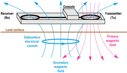
The frequency domain electromagnetic method (modified from Teeple and others, 2009c; Teeple, 2017).
In January and August 2022, a hand-held GEM-2 electromagnetic sensor was used to collect FDEM sounding data representing 15 frequencies (810; 1,110; 1,530; 2,070; 2,850; 3,930; 5,370; 7,290; 9,990; 13,710; 18,810; 25,710; 35,250; 48,270; and 66,090 hertz [Hz]) at the site along with 60-Hz FDEM sounding data as quality control to aid in identifying areas that may be affected by nearby power lines (Geophex, Ltd., 2024) (fig. 7). The GEM-2 sensor is a broadband, multifrequency, fixed-coil electromagnetic induction unit that can collect multiple frequencies simultaneously, and the deployment of this unit is relatively quick (a tool typically carried or mobilized on wheels during collection) (Geophex, Ltd., 2024). FDEM soundings were collected at the default interval of 1 Hz while the instrument was held approximately 3 ft above land surface. A Trimble DSM 232 GPS receiver (Trimble Inc., 2006) was used to georeference each FDEM sounding with a spatial coordinate. A detailed discussion of the GEM-2 and FDEM data theory is provided in Geophex, Ltd. (2024).
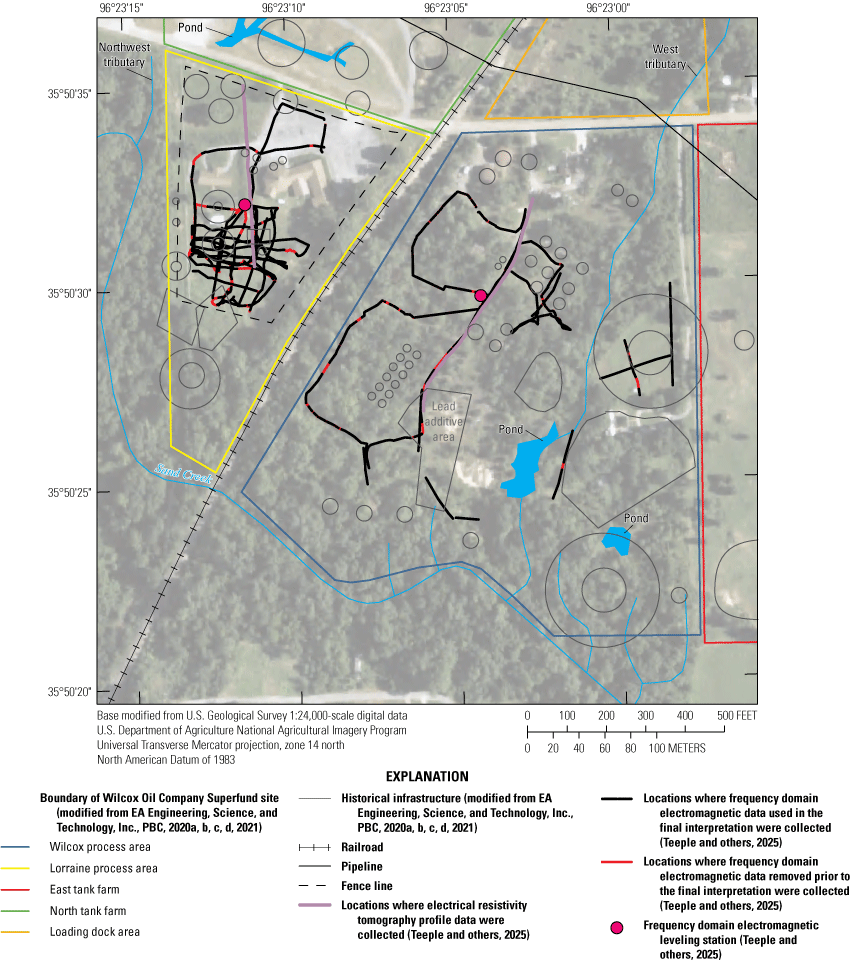
Locations where frequency domain electromagnetic and electrical resistivity tomography profile data were collected and leveling station locations in the Wilcox and Lorraine process areas of the Wilcox Oil Company Superfund site near Bristow, Creek County, Oklahoma, January and August 2022.
Over the course of collecting measurements with the GEM-2 sensor, the instrument has the potential for drift because of battery voltage depletion or temperature variations (Abraham and others, 2006). To account for drift correction, FDEM leveling stations (fig. 7) were established and occupied at the beginning, end, and regularly throughout the survey to compare static measurements over time to a single reference measurement. This loop-closure technique was adapted from the methods discussed in Abraham and others (2006). In January, a reconnaissance FDEM dataset was collected prior to the start of the study to test the feasibility of the method at the site. Leveling stations were not established for this feasibility dataset; therefore, a drift correction was not applied. It was observed that the changes (if any) from drift in that dataset were negligible and had a minimal impact on the final results.
The raw in-phase and quadrature responses of the FDEM data were reviewed to remove any data values that deviated excessively from surrounding values because of electromagnetic noise. First, a factor of 1.25 times the central tendency of the entire dataset was used to remove sequential outliers consisting of five values or less. Any values that were identified as outliers were replaced with a value representing the central tendency. The next step was to remove any remaining outliers by analyzing sequential runs of 11 data values. For this step, a trimmed mean was computed for each sequential run of 11 data values; the trimmed mean removed the highest and lowest 5 percent (totaling 10 percent) of the in-phase and quadrature response values before a mean was computed. After this processing of the raw data was completed, a drift correction was applied by using a linear correction calculated from the difference between static measurements of the in-phase and quadrature responses at the leveling stations. The three lowest frequencies (810; 1,110; and 1,530 Hz) were determined to be too “noisy” or variable to obtain any usable data for interpretation, so all data from these three lowest frequencies were removed from the dataset prior to any further processing. Examples of the raw and processed in-phase and quadrature responses are provided (fig. 8).
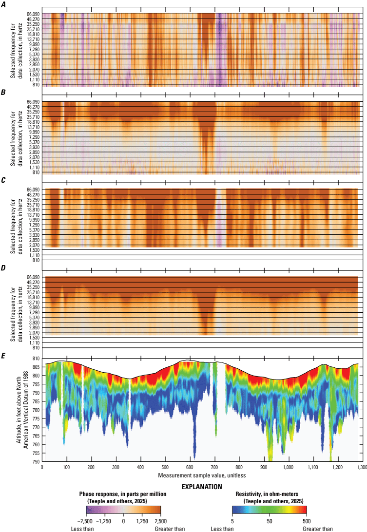
Examples of raw (A) in-phase and (B) quadrature responses; processed (C) in-phase and (D) quadrature responses; and (E) inverse modeling results of the processed frequency domain electromagnetic data collected in the Wilcox and Lorraine process areas of the Wilcox Oil Company Superfund site near Bristow, Creek County, Oklahoma, August 2022.
Because the GEM-2 sensor only records relative changes in apparent resistivity, the data required calibration to reference the “true” electrical response of earth material. The “true” in-phase and quadrature responses were calculated from the layered-earth resistivity model obtained from the ERT data described in the “Electrical Resistivity Tomography” section of this report. The depth and resistivity values from the final layered-earth model were used to back-calculate the in-phase and quadrature responses for the frequencies used by the GEM-2 sensor during FDEM data collection. The filtered and drift-corrected in-phase (fig. 8C) and quadrature (fig. 8D) values obtained by using the GEM-2 sensor were shifted to match the in-phase and quadrature responses from the layered-earth resistivity model results. In this manner, the relative changes in apparent resistivity measured by using the GEM-2 sensor were calibrated to the modeled (best-fit) electrical response of earth material. Apparent resistivity values were calculated for each frequency of the FDEM data by using these calibrated in-phase and quadrature responses. Further explanation of how apparent resistivity values are calculated from the in-phase and quadrature responses is provided by Huang and Won (2000).
Inverse modeling is the process of estimating the spatial distribution of subsurface resistivity from the measured in-phase and quadrature responses. The WinGEMv3 inversion program, developed by Geophex, Ltd. (2024), was used for inverse modeling of the FDEM soundings. Ten-layered models with initial thicknesses increasing with depth (resulting in a total depth of about 10.0 m) and initial resistivity values of 100 ohm-meters (ohm-m) were used as the starting models for the inversion process. The inversion program determines the calculated system response of these ten-layered models—the calculated apparent resistivities—as they are updated. The inversion program attempts to replicate the field data by altering the simulated thickness (depth) and resistivity values and recalculating the apparent resistivities in a series of iterations. The final models represent nonunique estimates of the true distribution of subsurface resistivity (fig. 8E). The final models were evaluated for anomalous resistivity values, and these values were removed from the dataset prior to the final interpretation (fig. 8E).
Electrical Resistivity Tomography
The ERT method uses an array of four electrodes (two Tx electrodes and two Rx electrodes) implanted into the ground to measure the bulk resistivity of the subsurface for a given point on the Earth’s surface (fig. 9). A known current was transmitted into the subsurface through the Tx electrodes, and the resulting electrical potential was measured as a voltage change between the two Rx electrodes. By increasing the distance between electrodes, the Tx current flows deeper into the subsurface, with the resulting voltage potential measured at the Rx electrodes representative of bulk electrical characteristics at greater depth. Using the known current and the measured voltage values, a resistance (the relative ability of earth material to transmit a current) was calculated by using Ohm’s law. The apparent resistivity of the subsurface was obtained by multiplying the resistance by a geometric factor dependent on the array geometry (Zohdy and others, 1974). A description of the ERT method and tables of the electrical properties of earth materials can be found in Zohdy and others (1974), Sumner (1976), Sharma (1997), Fitterman and Labson (2005), and Lucius and others (2007).
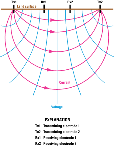
The electrical resistivity tomography method (modified from Teeple, 2017).
In August 2022, an IRIS Syscal Pro (IRIS Instruments, Orléans, France) 96-electrode unit resistivity meter was used to collect resistivity data from a reciprocal Schlumberger array (Tx electrodes located between Rx electrodes in a straight line), a Schlumberger array (Rx electrodes located between Tx electrodes in a straight line), and a forward and reverse dipole-dipole array (a Tx pair followed by an Rx pair in a straight line) (Zohdy and others, 1974). Two ERT profiles with electrodes spaced every 2 m were collected at the site: one in the Wilcox process area that was 192 m in length and one in the Lorraine process area that was 144 m in length. Each electrode was geospatially referenced with coordinates collected from an RTK GPS receiver. More discussion on ERT surveying and array configurations can be found in Burton and others (2014).
The raw data were imported into Prosys II software (IRIS Instruments, Orléans, France) (fig. 10A). The apparent resistivity values for each of the arrays were visually compared among each other as a quality check for reproducibility of the measurement. Although noisy (highly variable) data were measured at the site, all of the arrays showed similar results. The topography for the ERT profiles was input into the arrays, and each of the arrays was filtered to remove any excess noise. The induced current, measured voltage, and calculated apparent resistivity values were evaluated if they were within reasonable ranges, removing outliers, if necessary; induced currents between 240 and 900 milliamps, measured voltages of less than 0 millivolts (for dipole-dipole arrays only), and calculated apparent resistivity values between 0 and 500 ohm-m were retained. Anomalous points were further removed by using the automatic removal options within the software, which rejects points that do not match the general trend. To help further reduce noise in the ERT profiles, all of the arrays were combined into an apparent resistivity profile, and an automatic filtering was done by the software on the combined dataset for each profile (fig. 10B).
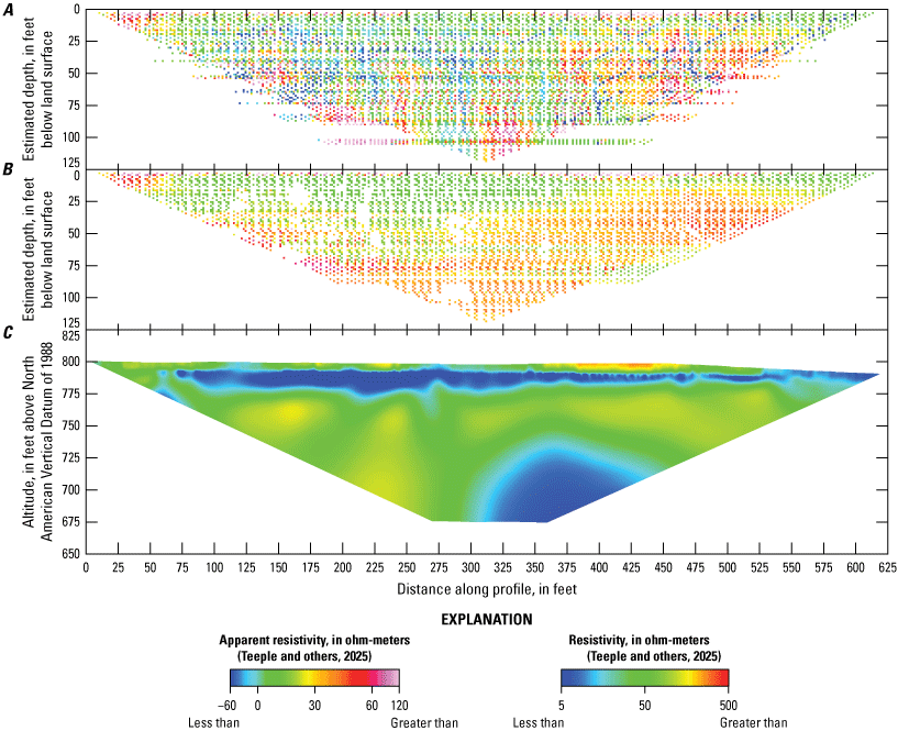
Examples of (A) raw and (B) filtered apparent resistivity data and (C) inverse modeling results for electrical resistivity tomography profile data collected in the Wilcox and Lorraine process areas of the Wilcox Oil Company Superfund site near Bristow, Creek County, Oklahoma, August 2022.
The filtered apparent resistivity data (fig. 10B) were processed and inverted with topographic data by using the finite-element method with least-squares estimation using RES2DINVx64 version 4.10.3 (Aarhus Geosoftware, Denmark). A 2D model consisting of multiple rectangular blocks, each assigned a centered resistivity value, was used by the program to determine electrical resistivity values for a nonuniform subsurface (Ball and others, 2006). The mean value of all apparent resistivities in the input data was selected as the starting apparent resistivity value for all model blocks. The inversion program determines the calculated system response of this 2D model—the calculated apparent resistivities—as the apparent resistivity values are updated. The inversion process iteratively calculates the system response to the numerical model of the subsurface distribution of resistivity with depth. The accuracy of the model is determined by comparing the absolute difference between the calculated model results with the measured data. The final 2D model represents a nonunique estimate of the true distribution of subsurface resistivity (fig. 10C). The inverse modeling process is described in detail by Loke (2004) and Advanced Geosciences, Inc. (2009).
Three-Dimensional Resistivity Grid Development
Land-surface altitudes were determined from the 3DEP DEM for all FDEM sounding locations and ERT electrode locations by using their horizontal coordinates to provide consistency and improve accuracy. Because of the similar depth and resistivity response by the borehole EC logging, FDEM soundings, and ERT profiles, the data were gridded together into a 3D grid by using Oasis montaj (Seequent, 2025) and the 3D-kriging method using the default kriging parameters for an exponential variogram model and a horizontal weighting factor of eight horizontal grid cells to one vertical grid cell (Seequent, 2020). The grid cell size used was a horizontal grid spacing of 5 by 5 m and a vertical spacing of 0.5 ft. For viewing on surface maps, 2D grids can be extracted from the 3D grid. The resistivity grid was iteratively compared to the inverse modeling results to evaluate outliers, grid accuracy, and clustered data. All outlier locations were evaluated through a correlation process to determine data-point uncertainty. The correlation process involved the comparison of gridded resistivity values to the inverse modeling results. Throughout the process, all resistivity values were reviewed and revised as needed to provide the best possible final representation of the inverse modeling results. The results from this 3D grid were compared to previously and newly collected subsurface data at the site.
Groundwater-Level Altitude Measurements
Prior to collecting groundwater-quality samples or slug tests, groundwater-level altitudes were measured at each well by following USGS methods described in Cunningham and Schalk (2011) (table 2). Electric tapes were used for all groundwater-level altitude measurements. Potentiometric-surface maps were created from the groundwater-level altitude data collected prior to collection of groundwater-quality samples during October–November 2022 to help assess spatial changes in groundwater-level altitudes across the study area (table 2). The groundwater-level altitude dataset collected prior to groundwater-quality sampling was used to develop the potentiometric-surface maps because it contained measurements from more wells compared to the groundwater-level altitude dataset collected prior to the slug tests; groundwater-level altitudes for the slug tests were only measured for the groundwater monitoring wells installed in 2022. Measured depths to the water table were converted to groundwater-level altitudes by subtracting the depths to the water table from the land-surface altitude at the well in feet above the North American Vertical Datum of 1988 (NAVD 88) (table 2). The potentiometric-surface grid was created by using a gridding method implemented in Oasis montaj (Seequent, 2025) referred to as the minimum curvature method (Webring, 1981; Seequent, 2020). The default gridding parameters included in Oasis montaj were used except tighter constraints were used on the acceptable difference between gridded and measured values in order to force more iterations, along with tighter constraints on the number of gridded values that meet this deviation requirement (Seequent, 2020). The maximum number of iterations for the gridding algorithm to converge to a solution was also increased (Seequent, 2020). The grid cell size used was a horizontal grid spacing of 15 by 15 m. All groundwater-level altitudes and the resulting grid were reviewed for the best possible final representation of the potentiometric surface. The groundwater-level altitude measurements for this study are available in a companion data release (Teeple and others, 2025).
Table 2.
Groundwater-level altitudes measured at each groundwater monitoring well or piezometer screened in the alluvial aquifer prior to collecting groundwater-quality samples or slug tests in the Wilcox and Lorraine process areas of the Wilcox Oil Company Superfund site near Bristow, Creek County, Oklahoma, October–December 2022.[Data from Teeple and others (2025). ID, identifier; ft, foot; NAVD 88, North American Vertical Datum of 1988; WL, groundwater-level; QW, groundwater-quality; bls, below land surface; ─, no data. Dates are in month/day/year format]
| Well ID (fig. 2) |
Altitude, in ft above NAVD 88 | Date of WL measurement prior to QW sampling | Depth of groundwater prior to QW sampling, in ft bls | WL altitude prior to QW sampling, in ft above NAVD 88 | Date of WL measurement prior to slug test | Depth of water prior to slug test, in ft bls | WL altitude prior to slug test, in ft above NAVD 88 |
|---|---|---|---|---|---|---|---|
| MW‑01 | 794.3 | 10/10/2022 | 6.96 | 787.3 | ─ | ─ | ─ |
| MW‑02 | 793.8 | 10/12/2022 | 115.94 | 1777.9 | ─ | ─ | ─ |
| MW‑03 | 800.1 | 10/10/2022 | 10.36 | 789.7 | ─ | ─ | ─ |
| MW‑04 | 794.1 | 10/11/2022 | 14.34 | 779.8 | ─ | ─ | ─ |
| MW‑05 | 786.9 | 10/12/2022 | 11.35 | 775.6 | ─ | ─ | ─ |
| MW‑06 | 779.0 | 10/13/2022 | 11.29 | 767.7 | ─ | ─ | ─ |
| PW‑01 | 785.6 | 10/13/2022 | 3.84 | 781.8 | ─ | ─ | ─ |
| PW‑02 | 785.3 | 11/1/2022 | 9.73 | 775.6 | ─ | ─ | ─ |
| PW‑03 | 785.3 | 10/13/2022 | 4.30 | 781.0 | ─ | ─ | ─ |
| PW‑04 | 794.0 | 10/10/2022 | 6.01 | 788.0 | ─ | ─ | ─ |
| LPA‑GW‑01 | 796.0 | 10/31/2022 | 6.50 | 789.5 | ─ | ─ | ─ |
| LPA‑GW‑02 | 798.6 | 10/31/2022 | ─2 | ─2 | ─ | ─ | ─ |
| LPA‑GW‑03 | 807.4 | ─ | Dry | ─ | ─ | ─ | ─ |
| WPA‑GW‑01 | 784.5 | 10/12/2022 | 13.06 | 771.4 | ─ | ─ | ─ |
| WPA‑GW‑04 | 792.3 | 10/11/2022 | 10.89 | 781.4 | ─ | ─ | ─ |
| WPA‑GW‑05 | 792.5 | 10/11/2022 | 11.80 | 780.7 | ─ | ─ | ─ |
| WPA‑GW‑06 | 793.3 | 10/31/2022 | 5.68 | 787.6 | ─ | ─ | ─ |
| WPA‑GW‑07 | 794.9 | 10/11/2022 | 11.85 | 783.1 | ─ | ─ | ─ |
| WPA‑GW‑09 | 797.4 | 10/12/2022 | 12.59 | 784.8 | ─ | ─ | ─ |
| USGS‑00 | 799.0 | ─ | Dry | ─ | 11/18/2022 | Dry | ─ |
| USGS‑01 | 788.4 | 11/2/2022 | 7.60 | 780.8 | 11/10/2022 | Dry | ─ |
| USGS‑02 | 790.9 | 10/31/2022 | 4.57 | 786.3 | 11/18/2022 | 4.66 | 786.2 |
| USGS‑04 | 792.6 | 11/1/2022 | 12.31 | 780.3 | 11/10/2022 | 11.34 | 781.3 |
| USGS‑05 | 801.5 | ─ | Dry | ─ | 11/8/2022 | Dry | ─ |
| USGS‑06 | 801.6 | 11/1/2022 | 18.84 | 1792.8 | 11/8/2022 | Dry | ─ |
| USGS‑07 | 796.1 | 10/31/2022 | 8.39 | 787.7 | 11/18/2022 | Dry | ─ |
| USGS‑08 | 800.4 | 10/31/2022 | 12.77 | 787.6 | 11/18/2022 | 13.39 | 787.0 |
| USGS‑09 | 795.6 | ─ | Dry | ─ | 11/18/2022 | Dry | ─ |
| USGS‑10 | 785.2 | 10/31/2022 | 16.08 | 769.1 | 11/10/2022 | 17.22 | 768.0 |
| USGS‑11 | 795.0 | 10/11/2022 | 7.45 | 787.6 | 12/8/2022 | 7.75 | 787.3 |
| USGS‑12 | 795.7 | 10/10/2022 | 7.74 | 788.0 | 12/8/2022 | 8.48 | 787.2 |
| USGS‑13 | 800.5 | 10/11/2022 | 6.24 | 794.3 | 12/8/2022 | 4.60 | 795.9 |
| USGS‑14 | 797.9 | 10/10/2022 | 8.22 | 789.7 | 12/8/2022 | 7.05 | 790.9 |
| USGS‑15 | 807.7 | 10/11/2022 | Dry | ─ | 12/8/2022 | 9.87 | 797.8 |
| USGS‑16 | 796.2 | 11/3/2022 | 6.90 | 789.3 | 11/18/2022 | 7.61 | 788.6 |
| USGS‑17 | 787.7 | 10/31/2022 | 15.47 | 772.2 | 11/10/2022 | 17.14 | 770.6 |
| USGS‑18 | 796.6 | 11/2/2022 | 8.65 | 788.0 | 11/10/2022 | 8.78 | 787.8 |
| USGS‑19 | 802.6 | 11/2/2022 | 9.11 | 793.5 | 11/18/2022 | 6.97 | 795.6 |
| USGS‑23 | 783.9 | 11/2/2022 | 10.84 | 773.1 | 11/10/2022 | 8.10 | 775.8 |
Groundwater-Quality Sampling
Groundwater-quality samples were collected from 33 wells during October–November 2022 (table 2). Of the existing wells at the site (table 1), six wells could not be sampled because those wells were dry or contained insufficient water. Samples were collected and shipped for laboratory analysis of VOCs, SVOCs, trace elements (including metals), major ions, natural attenuation parameters, and natural attenuation biomarkers. Sample collection and analysis methods and the quality-assurance and quality-control procedures used to collect, analyze, and verify the data are outlined in this section of the report.
Sample Collection and Analysis
Groundwater-quality samples were collected by following protocols for low-flow groundwater sampling (Puls and Barcelona, 1996). Samples were collected by using a peristaltic pump with dedicated polytetrafluoroethylene-lined tubing. Wells were purged of groundwater within the well column to ensure that groundwater being sampled was representative of the aquifer. During well purging, field properties (DO concentration, ORP, pH, specific conductance, groundwater temperature, and turbidity) were measured and recorded with an In-Situ AquaTroll 600 multiparameter sonde (In-Situ Inc., 2023a) and a Hach 2100Q portable turbidity meter (Hach, 2023). Because the turbidity values in the in-situ water in some wells were higher than the operational range of the Hach turbidity meter, turbidity was measured with the AquaTroll 600 multiparameter sonde at those wells. A well was considered stable and the purging of the well ceased when the field properties were within the criteria established in Puls and Barcelona (1996) for three consecutive measurements. Because of low recharge rates, some wells were completely dewatered during stabilization of field properties or during sample collection. At wells PW-01, PW-02, WPA-GW-04, WPA-GW-06, USGS-01, USGS-06, USGS-07, and USGS-18, (fig. 2; table 3), there was not enough groundwater volume available to obtain more than three consecutive stabilizations of field-property readings. If a well was dewatered during purging or sampling, the well was left to recharge overnight, and sampling was continued the following day, when possible, without recording field properties. Because these wells had already been pumped dry, any recharge was presumed to be representative of the aquifer. Sample dates and times for each groundwater-quality constituent group collected are available in Teeple and others (2025).
Table 3.
Selected water-quality properties measured in the samples collected from each groundwater monitoring well or piezometer in the Wilcox and Lorraine process areas of the Wilcox Oil Company Superfund site near Bristow, Creek County, Oklahoma, October–November 2022.[Data from Teeple and others (2025). ID, identifier; VOC, volatile organic compound; SVOC, semivolatile organic compound; ORP, oxygen-reduction potential; DO, dissolved oxygen; SC, specific conductance; X, sample collected; ─, not sampled]
| Well ID (fig. 2) |
Laboratory analysis | Field measurement | ||||||||
|---|---|---|---|---|---|---|---|---|---|---|
| VOCs | SVOCs | Trace elements | Nitrate and nitrite | Sulfate | Methane | Microbial community | Stabilization field properties (pH, ORP, DO, SC, temperature, and turbidity) | Ferrous iron | Sulfide | |
| MW‑01 | X | X | X | X | X | X | X | X | X | X |
| MW‑03 | X | X | X | X | X | X | X | X | X | X |
| MW‑04 | X | X | X | X | X | X | X | X | X | X |
| MW‑05 | X | X | X | X | X | X | X | X | X | X |
| MW‑06 | X | X | X | X | X | X | ─ | X | X | X |
| PW‑01 | ─ | ─ | ─ | X | X | ─ | X | ─ | ─ | ─ |
| PW‑02 | X | ─ | ─ | ─ | ─ | ─ | X | ─ | ─ | ─ |
| PW‑03 | X | X | ─ | ─ | ─ | ─ | ─ | X | ─ | ─ |
| PW‑04 | X | X | ─ | ─ | ─ | ─ | X | X | ─ | ─ |
| LPA‑GW‑01 | X | ─ | X | ─ | ─ | ─ | X | X | ─ | ─ |
| LPA‑GW‑02 | X | X | X | X | X | X | X | X | X | X |
| WPA‑GW‑01 | X | X | X | X | X | X | X | X | X | X |
| WPA‑GW‑04 | X | ─ | ─ | ─ | ─ | ─ | X | ─ | ─ | ─ |
| WPA‑GW‑05 | X | X | X | X | X | X | X | X | X | X |
| WPA‑GW‑06 | X | ─ | X | X | X | X | X | ─ | ─ | ─ |
| WPA‑GW‑07 | X | X | X | X | X | X | X | X | X | X |
| WPA‑GW‑09 | X | ─ | X | ─ | ─ | ─ | X | X | ─ | ─ |
| USGS‑01 | X | ─ | X | ─ | ─ | X | X | ─ | ─ | ─ |
| USGS‑02 | X | ─ | X | X | X | ─ | X | X | ─ | ─ |
| USGS‑04 | X | X | X | X | X | X | X | X | X | ─ |
| USGS‑06 | ─ | ─ | ─ | ─ | ─ | ─ | X | ─ | ─ | ─ |
| USGS‑07 | ─ | ─ | ─ | ─ | ─ | ─ | X | ─ | ─ | ─ |
| USGS‑08 | X | ─ | X | ─ | ─ | X | X | X | ─ | ─ |
| USGS‑10 | X | ─ | X | X | ─ | X | X | X | X | X |
| USGS‑11 | X | X | X | ─ | ─ | ─ | X | X | ─ | ─ |
| USGS‑12 | X | X | X | ─ | ─ | ─ | X | X | ─ | ─ |
| USGS‑13 | X | X | X | ─ | ─ | ─ | X | X | ─ | ─ |
| USGS‑14 | X | X | X | X | X | X | X | X | X | X |
| USGS‑16 | X | X | X | X | X | X | X | X | X | X |
| USGS‑17 | X | ─ | X | X | ─ | X | X | X | ─ | ─ |
| USGS‑18 | ─ | ─ | ─ | ─ | ─ | ─ | X | ─ | ─ | ─ |
| USGS‑19 | X | X | X | X | X | X | X | X | ─ | ─ |
| USGS‑23 | X | X | X | X | X | X | X | X | ─ | ─ |
USGS standard protocols, as described in the “National Field Manual for the Collection of Water-Quality Data” (USGS, variously dated), were followed for decontaminating equipment and collecting and processing groundwater samples except as noted in this section. Because of slow recharge rates, the groundwater-quality properties sampled at each well were dependent on the volume of water available in a given well. Because of these limitations, the order of sample collection was modified from standard USGS sampling protocols to ensure that samples for prioritized groundwater-quality properties were collected first. Samples were collected in the following order: microbial community samples, VOCs, SVOCs, trace elements, methane (because of its lower photochemical reactivity compared to other VOCs, methane is treated separately), and major ions, including nitrate, nitrite, and sulfate (the major ions analyzed at the site that will be discussed in this report). If a sample for a specific groundwater-quality constituent could not be collected because of volume limitations, a sample requiring less volume for the next group on the priority list was collected. When possible, Vacu-vials test kits (CHEMetrics, 2023) were used in the field to measure ferrous iron and sulfide concentrations. Groundwater-quality constituents measured at each well are summarized in table 3.
Groundwater-quality samples for VOCs, SVOCs, and trace elements were preserved, chilled on ice, and shipped within 24 hours to the EPA Region 6 Houston Laboratory in Houston, Texas, for analysis. Methods for the analysis of VOCs, SVOCs, and trace elements are documented in a series of EPA reports (EPA, 2014, 2017b, 2018b, 2018c). Samples for major ions (including nitrate, nitrite, and sulfate) were filtered by using a 0.45-micron pore size filter, chilled on ice, and shipped within 24 hours to the USGS National Water Quality Laboratory in Lakewood, Colorado, for analysis. Methods for the analysis of major ions are documented in Fishman and Friedman (1989) and Patton and Kryskalla (2011). Samples for methane were chilled on ice and submitted at the end of each sampling week to the SGS North America, Inc., laboratory in Orlando, Florida. Methods for the analysis of methane are documented in Hudson (2004). Samples for microbial community analysis were frozen and shipped to Microbiome Insights, Inc., in Vancouver, British Columbia, Canada, for sequencing of the 16S ribosomal ribonucleic acid (16S rRNA) gene to obtain abundance estimates of the microbial community. Community sequence data were processed by the Microbiome Insights, Inc., laboratory by using an Illumina MiSeq sequencing platform (Kozich and others, 2013) and the mothur software package (Schloss and others, 2009). Classification was completed using the SILVA 138 reference database (Quast and others, 2012).
Quality-Assurance and Quality-Control Procedures
To evaluate the variability of sample processing and analysis in groundwater-quality constituents, data from field-replicate samples were considered. A total of three replicate samples were collected and analyzed for VOCs and SVOCs, and two replicate samples were collected and analyzed for trace elements. Replicate samples were only used to assess variability when results were greater than or equal to the method detection limit. Data from the quality-control samples are available in Teeple and others (2025). To determine variability in environmental samples, the relative percent difference (RPD) between each pair of replicate samples was calculated by using the following equation:
whereC1
is the constituent concentration in the environmental sample, and
C2
is the constituent concentration in the replicate sample.
The RPDs for VOCs and SVOCs were evaluated first. RPDs for VOC replicate pairs ranged from 0.9 to 19.7 percent. The RPDs for eight of the nine constituents detected in VOC replicate pairs were less than 15 percent, indicating relatively low variability. For SVOCs, RPDs ranged from 0 to 100 percent. RPDs exceeded 30 percent for 9 of 18 SVOC constituents that were detected in replicate pairs. For five of these SVOC constituents, the concentrations were reported as estimated because results exceeded the calibration range, a failure in surrogate recovery during laboratory analysis was documented, or an internal standard exceeded the lower limit measured in samples. In the remaining nine replicate pairs, low concentrations of SVOCs (less than 4 µg/L) yielded RPDs greater than 30 percent; small differences in paired low concentration values of less than 4 µg/L in replicate samples inherently yield such relatively large RPDs.
RPDs for trace element replicate pairs were evaluated for replicate samples collected from wells MW-04 and MW-03 (fig. 2; table 1). The RPDs ranged from 0.8 to 98.1 percent for trace element replicate pairs. RPDs greater than 30 percent were calculated for 9 of 14 trace elements detected in replicate pairs, indicating high variability. All trace elements with high RPDs were measured in a sample collected from well MW-04. Although field properties had stabilized when groundwater-quality samples were collected, it is possible that a change in groundwater conditions as a result of groundwater withdrawals occurred between the collection of the environmental sample and the replicate sample. Because of possible changes in the groundwater withdrawal conditions, trace element results from samples collected at well MW-04 were flagged with a quality indicator to indicate the degree of questionable precision and accuracy of the value. Because the amount of variability in the replicate pair of samples collected from well MW-03 was deemed acceptable, no other trace element samples were qualified.
An equipment blank sample and trip blank samples were part of the sampling design. An equipment blank sample was collected and analyzed for VOCs, SVOCs, and trace elements, and five trip blanks were collected and analyzed for VOCs. The equipment blank sample was collected and analyzed to assess the potential bias resulting from contamination associated with environmental conditions, collection and processing procedures, equipment cleaning, transport, and laboratory analysis. Trip blank samples were collected and analyzed to assess the potential contamination associated with transport of samples from the field to the laboratory. None of the constituents analyzed were detected in the equipment blank sample or trip blank samples, thereby indicating that field and analytical procedures did not bias reported concentrations.
Slug Tests
In November and December 2022, following groundwater monitoring well development and groundwater-quality sampling, slug tests were completed on each of the groundwater monitoring wells installed in 2022 to (1) determine if the wells were in good hydraulic connection with the aquifer and (2) estimate the hydraulic conductivity of the aquifer at each well (table 4). Hydraulic conductivity is a measure of the ability of a porous material to allow fluids to pass through it. Higher hydraulic conductivity values correlate with higher yields and less drawdown in a well (Heath, 1983). A slug test requires a rapid change in groundwater level, usually as a result of adding or removing a known volume, or “slug,” into or from the well and then measuring the rate at which the groundwater level returns to static conditions (Cunningham and Schalk, 2011). Because of the slow recharge observed in the wells during groundwater-quality sampling, slug tests were determined to be the ideal method for testing the groundwater monitoring wells; the alternative of completing pump tests may have resulted in pumping the groundwater monitoring wells dry. The slug-test procedures were modified from Cunningham and Schalk (2011).
Table 4.
Summary of slug-test results from the groundwater monitoring wells screened in the alluvial aquifer in the Wilcox and Lorraine process areas of the Wilcox Oil Company Superfund site near Bristow, Creek County, Oklahoma, November and December 2022.[Data from Teeple and others (2025). ID, identifier; WL, groundwater level; ft, foot; bls, below land surface; ft/d, foot per day, ─, no data. Dates are in month/day/year format]
| Well ID (fig. 2) | Date of test | Estimated depth to “static” WL for test run 1, in ft bls1 | Hydraulic conductivity from test run 1, in ft/d | Estimated depth to “static” WL for test run 2, in ft bls1 | Hydraulic conductivity from test run 2, in ft/d | Estimated depth to “static” WL for test run 3, in ft bls1 | Hydraulic conductivity from test run 3, in ft/d | Appears to converge to a “static” WL1 | Final hydraulic conductivity, in ft/d |
|---|---|---|---|---|---|---|---|---|---|
| USGS‑00 | 11/18/2022 | −0.17 | 0.6 | −2.66 | 0.2 | ─ | ─ | No | ─ |
| USGS‑01 | 11/10/2022 | 0.34 | 0.1 | −2.24 | 0.2 | ─ | ─ | No | ─ |
| USGS‑02 | 11/18/2022 | 1.99 | 0.7 | 0.32 | 0.5 | 0.28 | 0.5 | Yes | 0.5 |
| USGS‑04 | 11/10/2022 | 8.01 | 0.1 | 8.28 | 0.04 | ─ | ─ | Yes | 0.04 |
| USGS‑05 | 11/8/2022 | 6.50 | 0.2 | 4.57 | 0.5 | 4.54 | 0.4 | Yes | 0.4 |
| USGS‑06 | 11/8/2022 | 1.78 | 0.01 | 0.87 | 0.02 | ─ | ─ | Yes | 0.02 |
| USGS‑07 | 11/18/2022 | 3.54 | 0.2 | 2.33 | 0.1 | ─ | ─ | Yes | 0.1 |
| USGS‑08 | 11/18/2022 | 4.66 | 0.03 | −1.17 | 0.5 | ─ | ─ | No | ─ |
| USGS‑09 | 11/18/2022 | 8.32 | 0.4 | 8.48 | 0.3 | ─ | ─ | Yes | 0.3 |
| USGS‑10 | 11/10/2022 | 5.71 | 0.03 | 3.29 | 0.05 | ─ | ─ | No | ─ |
| USGS‑11 | 12/8/2022 | 3.71 | 0.2 | 3.74 | 0.2 | ─ | ─ | Yes | 0.2 |
| USGS‑12 | 12/8/2022 | 3.06 | 0.1 | 2.92 | 0.09 | ─ | ─ | Yes | 0.09 |
| USGS‑13 | 12/8/2022 | −0.64 | 0.4 | 4.31 | 0.009 | ─ | ─ | No | ─ |
| USGS‑14 | 12/8/2022 | 2.10 | 0.01 | 2.17 | 0.01 | ─ | ─ | Yes | 0.01 |
| USGS‑15 | 12/8/2022 | 9.23 | 0.3 | 9.41 | 0.3 | ─ | ─ | Yes | 0.3 |
| USGS‑16 | 11/18/2022 | 6.89 | 0.2 | 6.87 | 0.1 | 6.88 | 0.1 | Yes | 0.1 |
| USGS‑17 | 11/10/2022 | 7.84 | 1 | 5.26 | 3 | 3.45 | 2 | No | ─ |
| USGS‑18 | 11/10/2022 | 7.91 | 0.3 | 4.47 | 0.4 | 5.98 | 0.2 | Yes | 0.2 |
| USGS‑19 | 11/18/2022 | 7.01 | 0.2 | 7.03 | 0.1 | 6.51 | 0.1 | Yes | 0.1 |
| USGS‑23 | 11/10/2022 | 7.07 | 0.02 | 6.93 | 0.02 | ─ | ─ | Yes | 0.02 |
Ideally, a slug test is performed when the groundwater-level altitude is above the top of the screened interval (Cunningham and Schalk, 2011). For almost all of the groundwater monitoring wells installed in 2022, this was not the case. A localized “static” groundwater level was estimated by filling the groundwater monitoring well with water and observing the change until a stationary level was reached and was above the screened interval. A Level TROLL 500 pressure transducer (In-Situ Inc., 2023b) was used to continuously log the groundwater level within the groundwater monitoring well at a 0.5-second interval. Prior to each slug test, the pressure transducer was lowered to the bottom of the groundwater monitoring well, and continuous logging was started. A known volume of water was immediately introduced into the groundwater monitoring well, and the groundwater level was recorded by the pressure transducer and simultaneously watched on a computer until the groundwater level had returned or almost returned to the localized “static” groundwater level. This process was repeated two to three times as separate test runs to evaluate the repeatability of the measurement. Data were downloaded from the pressure transducer by using Win-Situ software, version 5.7.8.0 (In-Situ Inc., Fort Collins, Colorado) and documented in a companion data release (Teeple and others, 2025). Data from the slug tests were analyzed by using the Bouwer-Rice method (Bouwer and Rice, 1976) and by assuming that the base of aquifer was at the bottom of the groundwater monitoring well if a depth of refusal was noted when the borehole for the well was drilled. The last test run at each groundwater monitoring well was used for the final interpretation of the site. The last test run was used because it provided the longest interval for the localized “static” groundwater level to equilibrate in the aquifer and will provide the most accurate representation of the hydraulic conductivity of the aquifer where the groundwater monitoring well was drilled.
Characterization of the Alluvial Aquifer
Data compiled and collected for the study were used to evaluate the characteristics of the alluvial aquifer at the site. These aquifer characteristics are defined by the hydrogeologic framework, groundwater-flow system, geochemistry, and hydraulic properties of the aquifer.
Hydrogeologic Framework
The term “hydrogeologic framework” as used in this report refers to the following geologic attributes that govern groundwater flow in the alluvial aquifer: land-surface altitude and orientation, bedrock altitude and orientation, overburden thickness, and sediment characteristics. The slope of the land surface helps to govern runoff from the site and recharge to the alluvial aquifer. Bedrock altitudes help to determine groundwater-flow paths, locations of inferred paleochannels important to groundwater flow, and the presence or absence of groundwater in a given location. Overburden thickness governs how quickly recharge reaches the alluvial aquifer and plays an important role in groundwater flow. The distribution of sediments (sand, silt, and clay) and the resistivity values of the sediments provide insights into the size and distribution of sediment particles in the subsurface that govern groundwater-flow characteristics and contaminant fate and transport.
The land surface in the Wilcox and Lorraine process areas generally slopes to the south and southwest towards Sand Creek (fig. 2). The lowest altitudes of the land surface are along stream channels in the depressions carved by Sand Creek and its west and northwest tributaries. In the Wilcox process area, the highest altitudes are in the northwest, and the topography slopes to the south and east to Sand Creek and its west tributary, respectively. In the Lorraine process area, the highest altitudes are in the northeast, and the topography slopes to the south and west to Sand Creek and its northwest tributary, respectively.
The altitudes to the top of bedrock have similar trends to those found in the land-surface topography. Bedrock is exposed or very near land surface to the north of the Wilcox and Lorraine process areas and generally slopes to the south and southwest towards Sand Creek (fig. 11). Similar to land surface, the lowest altitudes of the top of bedrock are found in the depressions carved by Sand Creek and its west and northwest tributaries. In the case of the west tributary, the depressions are not located directly below the stream; they are present on either side of the stream. The locations of the depressions likely indicate that the tributary has historically incised what appear to be two paleochannels into the bedrock. The inferred paleochannel to the east of the west tributary has deeper depressions than the inferred paleochannel to the west. In the Wilcox process area, the highest altitudes of the top of bedrock are in the northwest, and the bedrock slopes to the south and east to Sand Creek and its west tributary, respectively. In the Lorraine process area, the highest altitudes of the top of bedrock are in the northeast, but there is another bedrock high near the center of the process area. There is a small depression in the northwest part of the Lorraine process area that may be a small paleochannel that trends to the west.
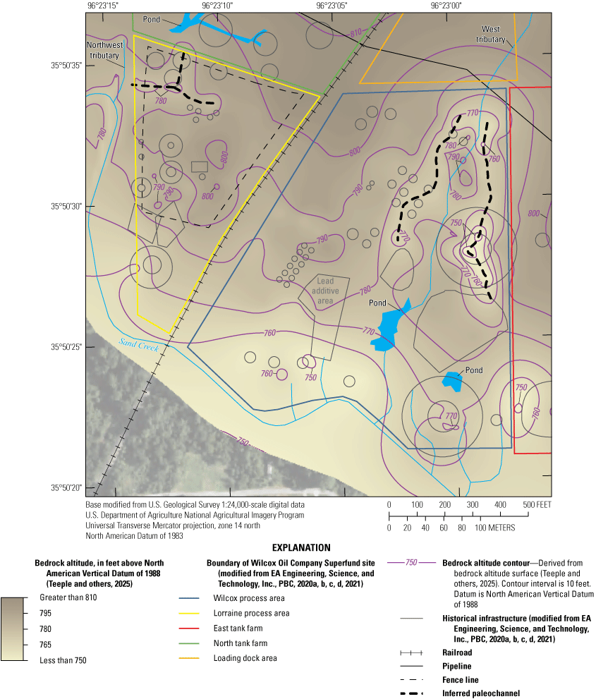
Altitudes of the top of bedrock in the Wilcox and Lorraine process areas of the Wilcox Oil Company Superfund site near Bristow, Creek County, Oklahoma.
An overburden thickness grid was computed by subtracting the altitudes of the bedrock surface grid from the land-surface topography (fig. 12). Because of the similar slopes between land surface (fig. 2) and the top of bedrock (fig. 11), locations with the thickest overburden occur where there are depressions in the bedrock typically related to inferred paleochannels (fig. 12). These locations coincide with Sand Creek and the locations of two inferred paleochannels on the east and west sides of the west tributary (fig. 12). In the Lorraine process area, there is thick overburden (greater than 20 ft) to the north (fig. 12) that would correlate with an apparent bedrock low between two bedrock highs (fig. 11).
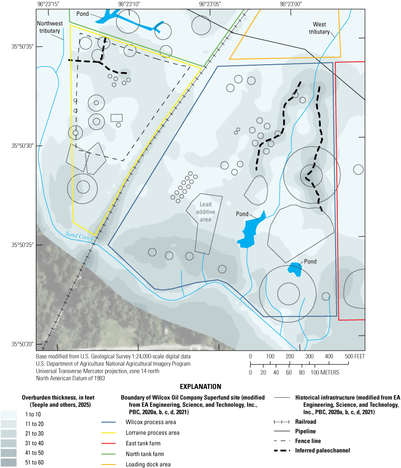
Overburden thickness in the Wilcox and Lorraine process areas of the Wilcox Oil Company Superfund site near Bristow, Creek County, Oklahoma.
The primary sediment observed within the overburden consisted of silt to sand-sized unconsolidated sediments that ranged from light brown to black. The borehole EC logging results were compared to the soil-core descriptions, and there appeared to be three major sediment groups: (1) a clay-dominant group with most of the resistivity values less than 100 ohm-m, (2) a sand-dominant group with most of the resistivity values greater than 200 ohm-m, and (3) a clay and sand mix group with most resistivity values between 100 and 200 ohm-m (figs. 13 and 14A). The combined 3D resistivity model results were compared to the soil-core descriptions as well, but because the combined 3D resistivity model statistically merges spatial resistivity results throughout the Wilcox and Lorraine process areas and incorporates multiple collection methods with different spatial resolutions, only bulk resistivity changes could be measured. Resistivity values for the clay-dominant group and sand-dominant group in the Wilcox and Lorraine process areas derived from the borehole EC logging results (fig. 14A) and combined 3D resistivity model showed good agreement (fig. 14B). However, resistivity values for the clay and sand mix group in the Wilcox and Lorraine process areas derived from the borehole EC logging results (fig. 14A) were higher than the resistivity values derived from the combined 3D resistivity model (fig. 14B). This difference between resistivity values derived from the borehole EC logging results and combined 3D resistivity model for the clay and sand mix group is attributed to the bulk resistivity values measured in the combined 3D resistivity model; resistivity values in the model have a gradual change across clay and sand boundaries instead of sharp changes as measured in the borehole EC logging results. In the combined 3D resistivity model, most resistivity values are greater than 140 ohm-m in the sand-dominant group, and most resistivity values are less than 100 ohm-m in the clay-dominant group (fig. 14B). It was assumed that resistivity values derived from the combined 3D resistivity model of 100 ohm-m represented at least an equal proportion of clay and sand and that resistivity values greater than 100 ohm-m represented the sand-dominant group.
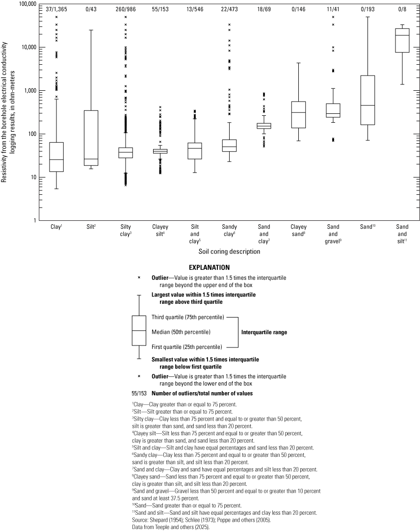
Boxplots of resistivity values derived from the borehole electrical conductivity logging results based on soil-core descriptions in the Wilcox and Lorraine process areas of the Wilcox Oil Company Superfund site near Bristow, Creek County, Oklahoma, October 2022.
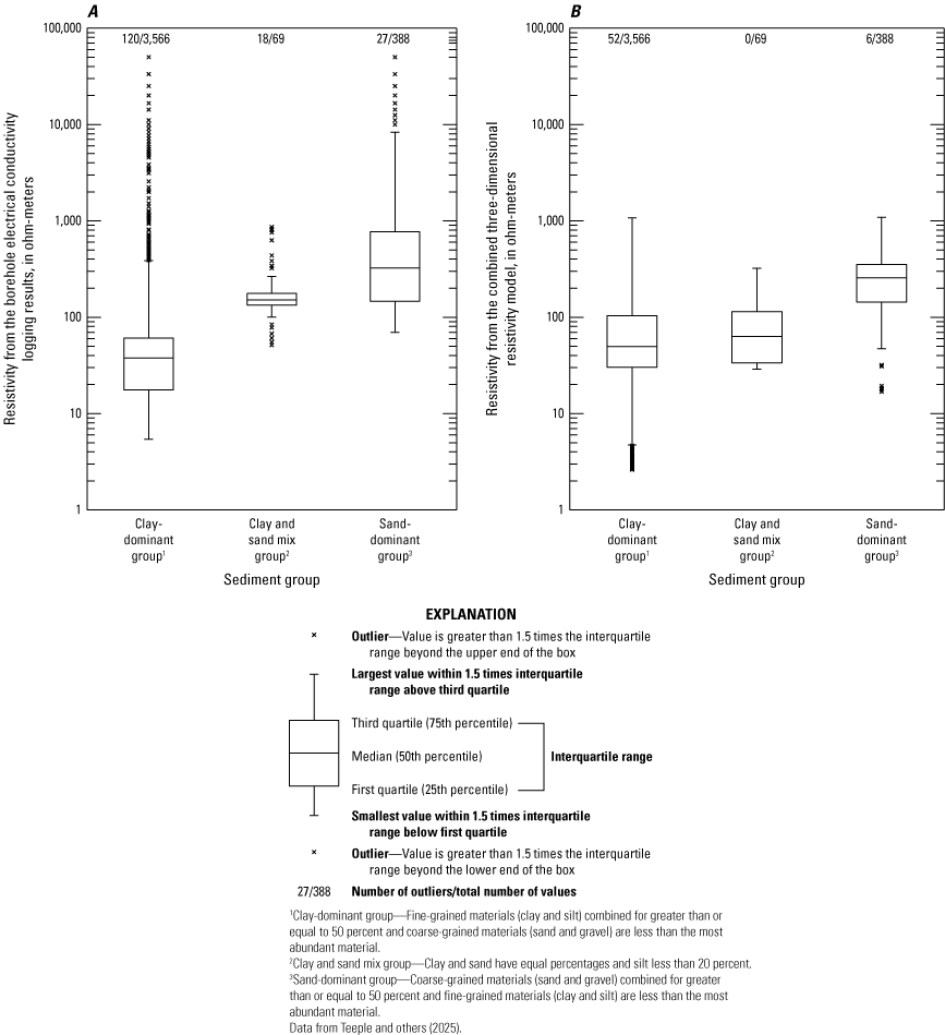
Boxplots of resistivity values derived (A) from the borehole electrical conductivity logging results and (B) from the combined three-dimensional resistivity model based on the major sediment groups in the Wilcox and Lorraine process areas of the Wilcox Oil Company Superfund site near Bristow, Creek County, Oklahoma, 2022.
Resistivity values of the sand-dominant group (resistivity values greater than 100 ohm-m) were extracted from the combined 3D resistivity model to gain a better understanding of locations of thicker sand layers in the Wilcox and Lorraine process areas. Figure 15 shows the estimated overall thickness of the sand-dominant group within the overburden, which might represent one sand layer, or multiple sand layers separated by clay-dominant group sediments; these sand-dominant group thicknesses are undifferentiated between these two scenarios. A sand-dominant group thickness within the overburden of less than or equal to 10 ft was evident in most (about 90 percent) of the gridded area (fig. 15). A comparatively thick sand-dominant group (greater than 15 ft thick in some areas) was mapped in the bedrock east of the west tributary to Sand Creek; this comparatively thick sand-dominant group coincides with the location of an inferred paleochannel (figs. 11 and 15).
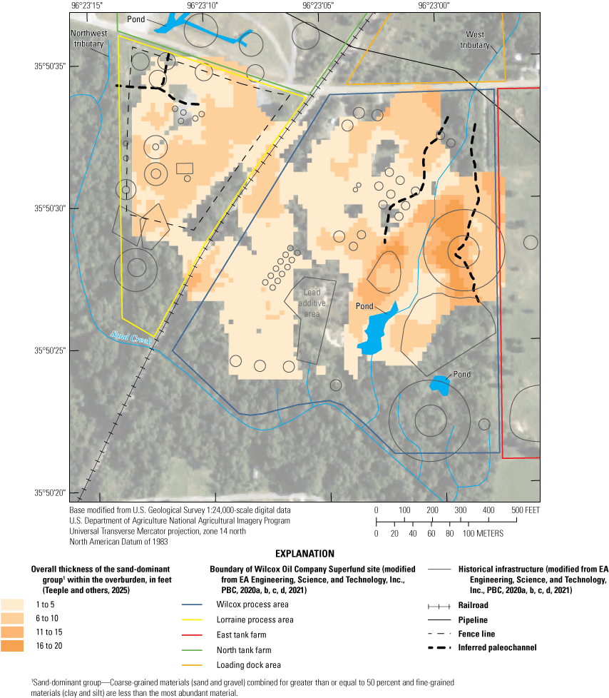
Overall thickness of the sand-dominant group identified in the combined three-dimensional resistivity model by values greater than 100 ohm-meters within the overburden in the Wilcox and Lorraine process areas of the Wilcox Oil Company Superfund site near Bristow, Creek County, Oklahoma, 2022.
Evaluating the mean normalized resistivity values for the sand-dominant parts of the overburden can potentially identify areas that contain a higher percentage of sand and gravel compared to fine-grained sediments (fig. 16). Resistivity values were converted to log values, a mean was calculated, and then the mean log value was recomputed to resistivity to obtain the mean normalized resistivity. In about 75 percent of the gridded area (fig. 15), the mean normalized resistivity values in the sand-dominant group were interpreted as being less than 210 ohm-m—a value similar to the lower particle size cutoff of the sand-dominant group of 200 ohm-m as defined by the borehole EC logging results (fig. 14A). Hence, in about 75 percent of the gridded area, the sand-dominant group thickness consists of relatively fine sand with some clay and silt mixed in, similar to that of the clay and sand mix group (resistivities between 100 and 200 ohm-m) (fig. 14A). Areas with mean normalized resistivity values greater than 210 ohm-m in the sand-dominant group thickness (fig. 16) are generally associated with areas of thin overburden (fig. 12). These high mean normalized resistivity values may indicate that the bedrock in these locations consists of exposed sandstone layers as opposed to the upper mudstone unit of the Barnsdall Formation; weathering of the interbedded layers of sandstone found in the Barnsdall Formation has likely resulted in an abundance of sandstone gravel and sand in these areas. In the northeastern part of the Wilcox process area, some of this weathered sandstone may have filled in the inferred paleochannels on either side of the west tributary (fig. 16).
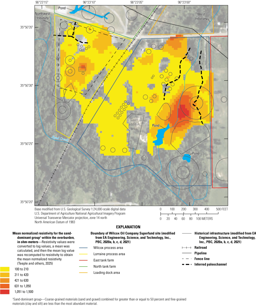
Mean normalized resistivity for the sand-dominant group within the overburden in the Wilcox and Lorraine process areas of the Wilcox Oil Company Superfund site near Bristow, Creek County, Oklahoma, 2022.
Groundwater-Flow System
Groundwater-level altitudes in the alluvial aquifer in the Wilcox and Lorraine process areas are affected by the overburden and bedrock altitudes (fig. 17). With such a thin overburden in the area (fig. 12), the presence of groundwater and the groundwater flow in the alluvial aquifer are highly dependent on the bedrock altitude (fig. 11). During October–November 2022, groundwater was absent in the north-central parts of the Wilcox and Lorraine process areas because the bedrock altitudes were higher than the groundwater-level altitudes in these parts (figs. 11, 17). The bedrock altitudes eventually became lower than the groundwater-level altitudes as the bedrock altitudes dipped towards the south to southwest and to the east in the Wilcox process area and to the west in the Lorraine process area. Groundwater-level altitudes could not be characterized in the southwestern part of the Wilcox process area and the southern part of the Lorraine process area because of a lack of groundwater-level altitude data for these parts.
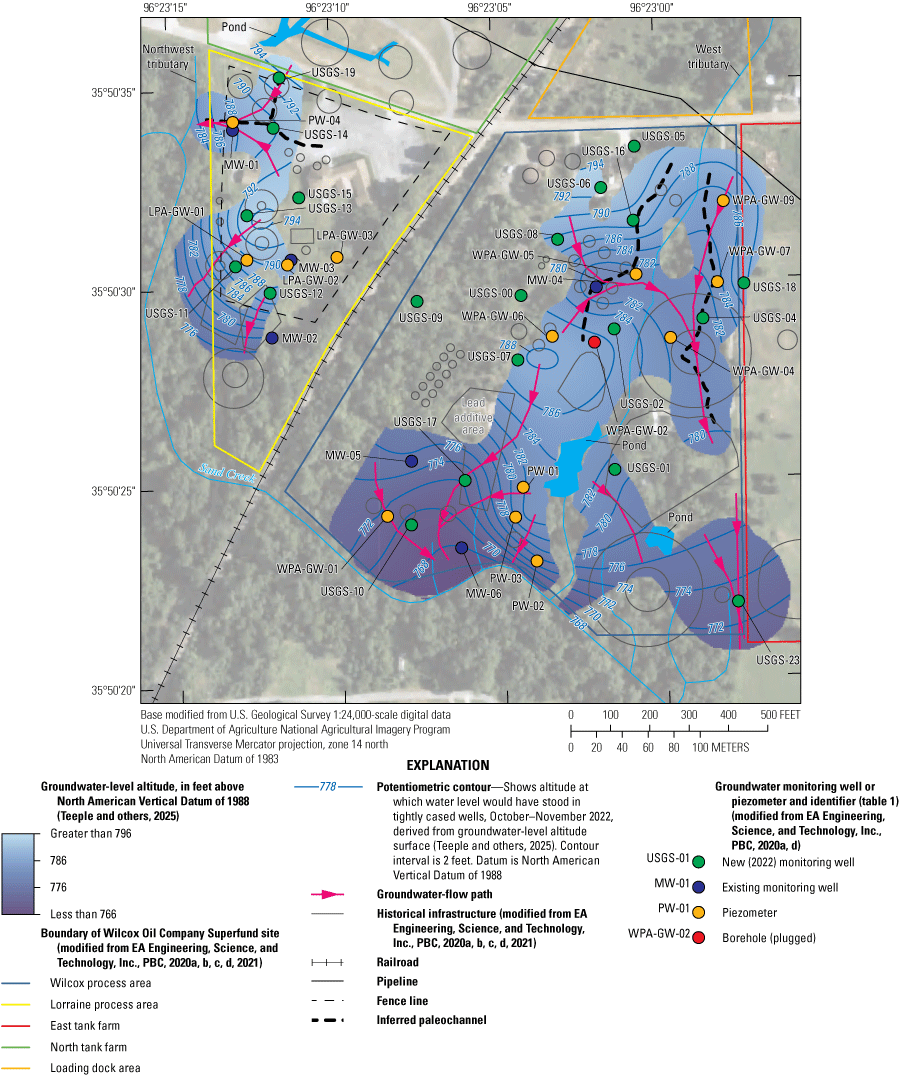
Groundwater-level altitudes in the alluvial aquifer in the Wilcox and Lorraine process areas of the Wilcox Oil Company Superfund site near Bristow, Creek County, Oklahoma, October–November 2022.
In general, groundwater flows south towards Sand Creek, although bedrock highs in the Wilcox and Lorraine process areas affect the flow of groundwater at more localized scales (fig. 17). In the Wilcox process area, there is a bedrock high in the central part of the process area that acts as a groundwater divide, causing groundwater to flow in opposite directions on either side of this high. Groundwater to the north of this divide flows east and then south, following the location of an inferred paleochannel east from the west tributary to Sand Creek in the south (fig. 17). Although not mapped in this report, the potential exists for disconnected pools of groundwater to form as precipitation is recharged in the depressions of the bedrock highs in the Wilcox and Lorraine process areas. A mapped disconnect in the groundwater-flow path east of well USGS-01 (fig. 17) may be an artifact caused by a lack of depth of refusal data for the area where interpolation from gridding resulted in higher top of bedrock altitudes in this area (fig. 11), and a hydraulic connection (groundwater-flow path) may in fact exist where a disconnect is mapped. Similar to the Wilcox process area, there is a bedrock high in the central part of the Lorraine process area that acts as a groundwater divide (fig. 17). Groundwater north of this divide follows separate flow paths that join and flow west towards the northwest tributary. Based on the groundwater-level altitudes measured during October–November 2022, the mean groundwater gradient in the Wilcox and Lorraine process areas is 0.04 ft/ft.
Geochemistry
Wells that were coincident with or proximal to bedrock highs (MW-02, LPA-GW-03, USGS-00, USGS-05, USGS-09, and USGS-15) were not sampled because they contained insufficient water (figs. 11, 17). For the wells that were sampled, groundwater results for VOCs, SVOCs, and trace elements were compared against screening levels established for the site by the EPA (EA Engineering, Science, and Technology, Inc., PBC, 2020a). The screening levels are based on either the MCL for a constituent, which is defined as the maximum level allowed of a contaminant in water delivered to any user of a public water system (EPA, 2023b), or the EPA Region 6 regional screening levels (RSLs) for tapwater (EPA, 2025) if an MCL for a particular constituent is not applicable (EA Engineering, Science, and Technology, Inc., PBC, 2020a).
Because of suspected high concentrations at well PW-03, samples for VOCs and SVOCs were diluted by a factor of 1,000 and 200, respectively, prior to analysis of all constituents in the schedules used by the laboratory. As a result, the reporting limits associated with VOC and SVOC analyses for samples collected from well PW-03 were various orders of magnitude higher than the reporting limits for samples collected from the remaining wells. The elevated reporting levels associated with well PW-03 may have prevented the detection of some of the VOCs and SVOCs present in the sample at concentrations lower than the reporting limit.
Volatile Organic Compounds
Groundwater samples for the analysis of VOCs were collected from 29 wells (table 3). VOCs were detected in the samples from 26 of these 29 wells, and the number of VOCs detected in the samples from a given well ranged from 1 to 8 (table 5). Of the 49 VOCs quantified, the concentrations of 6 VOCs exceeded their respective screening levels in samples collected from 1 or more wells (table 6). Methylcyclohexane, a solvent (EPA, 1984), was the most frequently detected VOC (detected in samples from 19 wells) with concentrations ranging from 0.6 to 684 µg/L; the maximum concentration of methylcyclohexane was measured in the sample collected from well USGS-16. The petroleum hydrocarbons cyclohexane and isopropylbenzene (EPA, 2009) were both detected in the samples collected from 15 wells. The concentrations of cyclohexane and isopropylbenzene ranged from 1.7 to 694 µg/L and from 2.5 to 61.8 µg/L, respectively. Concentrations of isopropylbenzene exceeded the screening level in the samples collected from wells MW-01 and MW-04 (table 6). Benzene, which is also a petroleum hydrocarbon (EPA, 2009), was detected at concentrations ranging from 1.0 to 3,300 µg/L in samples collected from 10 wells. The screening level for benzene was exceeded in the samples collected from seven wells (fig. 18). All six VOCs that exceeded their respective screening levels (benzene, ethylbenzene, isopropylbenzene, meta- and (or) para-xylene, ortho-xylene, and toluene) had maximum concentration for these constituents measured at well MW-04 (table 6).
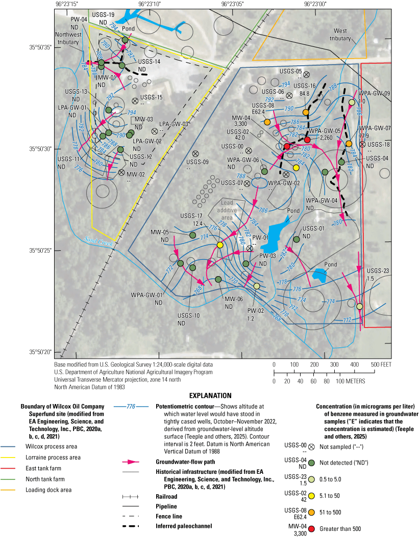
Concentrations of benzene measured in samples collected from groundwater monitoring wells or piezometers in the Wilcox and Lorraine process areas of the Wilcox Oil Company Superfund site near Bristow, Creek County, Oklahoma, October–November 2022.
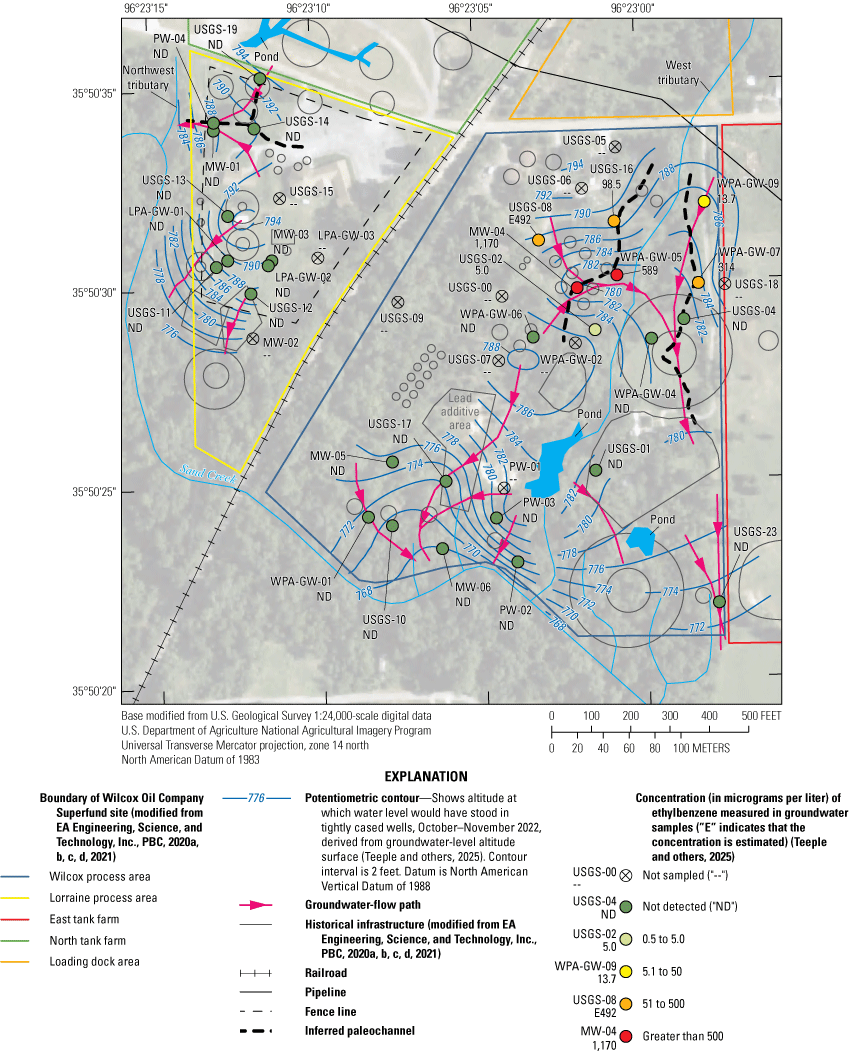
Concentrations of ethylbenzene measured in samples collected from groundwater monitoring wells or piezometers in the Wilcox and Lorraine process areas of the Wilcox Oil Company Superfund site near Bristow, Creek County, Oklahoma, October–November 2022.
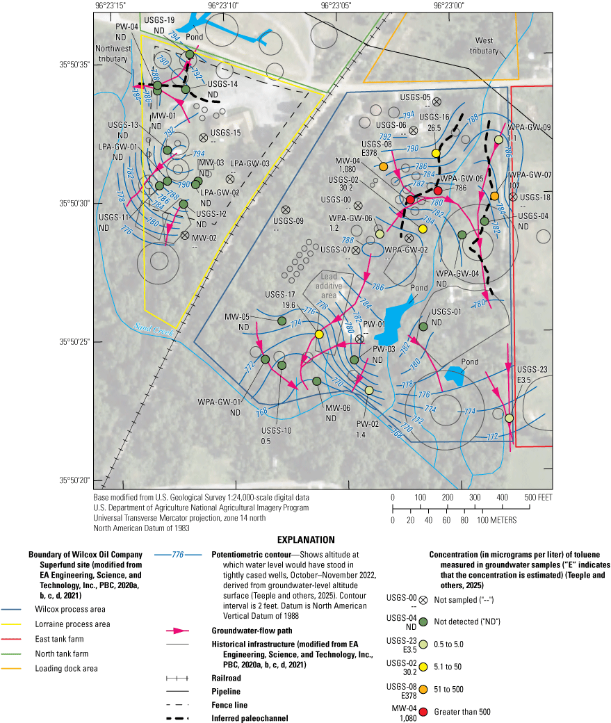
Concentrations of toluene measured in samples collected from groundwater monitoring wells or piezometers in the Wilcox and Lorraine process areas of the Wilcox Oil Company Superfund site near Bristow, Creek County, Oklahoma, October–November 2022.
Table 5.
Number of volatile and semivolatile organic compounds detected in samples collected from groundwater monitoring wells or piezometers in the Wilcox and Lorraine process areas of the Wilcox Oil Company Superfund site near Bristow, Creek County, Oklahoma, October–November 2022.[Data from Teeple and others (2025). ID, identifier; VOC, volatile organic compound; SVOC, semivolatile organic compound; ─, not sampled]
| Well ID (figs. 2 and 17–20) |
Number of VOCs detected | Number of SVOCs detected |
|---|---|---|
| MW-01 | 3 | 7 |
| MW-03 | 0 | 1 |
| MW-04 | 8 | 18 |
| MW-05 | 1 | 0 |
| MW-06 | 0 | 0 |
| PW-02 | 8 | ─ |
| PW-03 | 0 | 4 |
| PW-04 | 3 | 14 |
| LPA-GW-01 | 2 | ─ |
| LPA-GW-02 | 3 | 6 |
| WPA-GW-01 | 1 | 4 |
| WPA-GW-04 | 2 | ─ |
| WPA-GW-05 | 8 | 14 |
| WPA-GW-06 | 4 | ─ |
| WPA-GW-07 | 8 | 5 |
| WPA-GW-09 | 8 | ─ |
| USGS-01 | 4 | ─ |
| USGS-02 | 8 | ─ |
| USGS-04 | 2 | 4 |
| USGS-08 | 8 | ─ |
| USGS-10 | 6 | ─ |
| USGS-11 | 5 | 7 |
| USGS-12 | 2 | 1 |
| USGS-13 | 4 | 5 |
| USGS-14 | 5 | 9 |
| USGS-16 | 7 | 13 |
| USGS-17 | 3 | ─ |
| USGS-19 | 4 | 8 |
| USGS-23 | 6 | 7 |
Table 6.
Volatile organic compounds detected in samples collected from groundwater monitoring wells or piezometers in the Wilcox and Lorraine process areas of the Wilcox Oil Company Superfund site near Bristow, Creek County, Oklahoma, October–November 2022.[Data from Teeple and others (2025). VOC, volatile organic compound; µg/L, microgram per liter; ID, identifier; MCL, maximum contaminant level (U.S. Environmental Protection Agency [EPA], 2023b); RSL, EPA Region 6 regional screening level for tapwater (EPA, 2025; EA Engineering, Science, and Technology, Inc., PBC, 2020a)]
| VOC | Number of detections | Minimum concentration, in µg/L | Maximum concentration, in µg/L | Well ID for well with maximum concentration (figs. 2 and 17–20) |
Screening level type | Screening level, in µg/L | Number of times screening level was exceeded |
|---|---|---|---|---|---|---|---|
| 1,2-dichloroethane | 1 | 1.3 | 1.3 | MW‑05 | MCL | 5.0 | 0 |
| 2-butanone | 5 | 5.7 | 11.6 | USGS‑11 | RSL | 560 | 0 |
| Acetone | 14 | 6.9 | 85.0 | USGS‑11 | RSL | 14,000 | 0 |
| Benzene | 10 | 1.0 | 3,300 | MW‑04 | MCL | 5.0 | 7 |
| Bromodichloromethane | 1 | 0.8 | 0.8 | USGS‑01 | RSL | 8.3 | 0 |
| Bromoform | 1 | 2.5 | 2.5 | USGS‑01 | MCL | 80 | 0 |
| Chloromethane | 4 | 0.5 | 0.9 | USGS‑04 | RSL | 19 | 0 |
| Cyclohexane | 15 | 1.7 | 694 | USGS‑16 | RSL | 13,000 | 0 |
| Dibromochloromethane | 2 | 0.5 | 2.4 | USGS‑01 | MCL | 80 | 0 |
| Ethylbenzene | 7 | 5.0 | 1,170 | MW‑04 | MCL | 700 | 1 |
| Isopropylbenzene | 15 | 2.5 | 61.8 | MW‑04 | RSL | 45 | 2 |
| meta-and (or) para-xylene | 8 | 2.9 | 1,970 | MW‑04 | RSL | 190 | 3 |
| Methylcyclohexane | 19 | 0.6 | 684 | USGS‑16 | RSL | 1,300 | 0 |
| Methylene chloride | 1 | 0.9 | 0.9 | USGS‑10 | MCL | 5.0 | 0 |
| ortho-xylene | 8 | 0.6 | 342 | MW‑04 | RSL | 190 | 1 |
| Toluene | 12 | 0.5 | 1,080 | MW‑04 | MCL | 1,000 | 1 |
The highest concentrations of VOCs among the constituents exceeding screening levels were typically measured in samples collected from wells in the northern part of the Wilcox process area, which includes wells MW-04 and WPA-GW-05. Periodic releases of contaminants into the soil in the Wilcox process area likely resulted in migration of these contaminants into the groundwater (EA Engineering, Science, and Technology, Inc., PBC, 2020a). Because of the direction of groundwater flow (figs. 18, 19, and 20), contaminants are likely to remain in the area surrounding well MW-04 with perhaps the potential to migrate east and south along the inferred paleochannel that is east of the west tributary to Sand Creek. These results are consistent with previous findings by EA Engineering, Science, and Technology, Inc., PBC, (2020a) in which the area surrounding well MW-04 had higher numbers of VOC detections and higher VOC concentrations compared to the areas surrounding other wells sampled. Because concentrations of VOCs did not typically exceed screening levels at wells outside of the vicinity of MW-04, results from this sampling event indicate that a plume of substantial areal extent has not developed at the site for VOCs.
Semivolatile Organic Compounds
Groundwater samples for the analysis of SVOCs were collected from 19 wells (table 3). SVOCs were detected in the samples from 17 wells, and the number of SVOCs detected in the samples from a given well ranged from 1 to 18 (table 5). Of the 70 constituents quantified by the analytical methods, 25 were detected in groundwater samples collected at the site (table 7). The compound 1-methylnaphthalene was detected at the highest frequency (detected in samples from 14 wells) with concentrations ranging from 0.2 to 75.5 µg/L, with the maximum concentration measured at well MW-04. There are no screening levels associated with 1-methylnaphthalene. In the samples from 13 wells, 2-methylnaphthalene was detected. The screening level of 36 µg/L for 2-methylnaphthalene was exceeded in the samples from five wells. Benzo(a)pyrene was detected in the samples from four wells with concentrations ranging from 0.1 to 0.4 µg/L (fig. 21). The screening level of 0.2 µg/L for benzo(a)pyrene was exceeded in the samples from wells MW-04 and PW-04. Naphthalene was detected in the samples from 12 wells with concentrations ranging from 0.3 to 154 µg/L (fig. 22). The screening level of 0.17 µg/L for naphthalene was exceeded in the samples from all wells in which naphthalene was detected, which included wells in the Lorraine process area. Extremely high concentrations of phenol (180,000 µg/L), and selected cresol compounds (2-methylphenol [782,000 µg/L], 2,4-dimethylphenol [868,000 µg/L], and 3- and (or) 4-methylphenol [714,000 µg/L]) were measured in the sample from well PW-03, resulting in exceedances of the EPA Region 6 RSLs for tapwater (EPA, 2025) for all constituents measured in samples collected from well PW-03.
Table 7.
Semivolatile organic compounds detected in samples collected from groundwater monitoring wells or piezometers in the Wilcox and Lorraine process areas of the Wilcox Oil Company Superfund site near Bristow, Creek County, Oklahoma, October–November 2022.[Data from Teeple and others (2025). SVOC, semivolatile organic compound; µg/L, microgram per liter; ID, identifier; ─, no data; RSL, U.S. Environmental Protection Agency [EPA] Region 6 regional screening level for tapwater (EPA, 2025; EA Engineering, Science, and Technology, Inc., PBC, 2020a); MCL, maximum contaminant level (EPA, 2023b)]
| SVOC | Number of detections | Minimum concentration, in µg/L | Maximum concentration, in µg/L | Well ID for well with maximum concentration (figs. 2, 17–22) |
Screening level type | Screening level, in µg/L | Number of times screening level was exceeded |
|---|---|---|---|---|---|---|---|
| 1-methylnaphthalene | 14 | 0.2 | 75.5 | MW‑04 | None | ─ | ─ |
| 1,1'-biphenyl | 2 | 1.6 | 1.9 | WPA‑GW‑05 | RSL | 0.083 | 2 |
| 2-methylnaphthalene | 13 | 0.2 | 103 | MW‑04 | RSL | 36 | 5 |
| 2-methylphenol1 | 1 | 782,000 | 782,000 | PW‑03 | RSL | 93 | 1 |
| 2,4-dimethylphenol1 | 3 | 10.5 | 868,000 | PW‑03 | RSL | 360 | 1 |
| 3- and (or) 4-methylphenol1 | 4 | 6.6 | 714,000 | PW‑03 | RSL | 190 | 1 |
| Acenaphthene | 9 | 0.2 | 1.1 | MW‑04 | RSL | 190 | 0 |
| Anthracene | 4 | 0.2 | 0.8 | MW‑04 | RSL | 1,800 | 0 |
| Benzo(a)anthracene | 3 | 0.2 | 1.0 | MW‑04 | RSL | 0.03 | 3 |
| Benzo(a)pyrene | 4 | 0.1 | 0.4 | MW‑04 | MCL | 0.2 | 2 |
| Benzo(b)fluoranthene | 2 | 0.1 | 0.3 | MW‑04 | RSL | 0.25 | 1 |
| Benzo(g,h,i)perylene | 2 | 0.2 | 0.2 | MW‑04 and PW‑04 | None | ─ | ─ |
| Bis(2-ethylhexyl) phthalate | 1 | 2.3 | 2.3 | PW‑04 | MCL | 6.0 | 0 |
| Caprolactam | 2 | 11.8 | 18.7 | USGS‑11 | RSL | 990 | 0 |
| Carbazole | 2 | 2.9 | 3.3 | WPA‑GW‑05 | None | ─ | ─ |
| Chrysene | 4 | 0.2 | 1.6 | MW‑04 | RSL | 25 | 0 |
| Di-n-butyl phthalate | 4 | 3.4 | 11.0 | USGS‑23 | RSL | 90 | 0 |
| Diethyl phthalate | 1 | 5.9 | 5.9 | USGS‑14 | RSL | 15,000 | 0 |
| Fluoranthene | 3 | 0.2 | 0.8 | MW‑04 | RSL | 800 | 0 |
| Fluorene | 13 | 0.2 | 3.0 | PW‑04 | RSL | 290 | 0 |
| Naphthalene | 12 | 0.3 | 154 | MW‑04 | RSL | 0.17 | 12 |
| Pentachlorophenol | 2 | 0.3 | 0.4 | USGS‑16 | RSL | 1.0 | 0 |
| Phenanthrene | 13 | 0.1 | 11.1 | MW‑04 | None | ─ | ─ |
| Phenol | 5 | 4.7 | 180,000 | PW‑03 | RSL | 5,800 | 1 |
| Pyrene | 4 | 0.6 | 3.5 | MW‑04 | RSL | 120 | 0 |
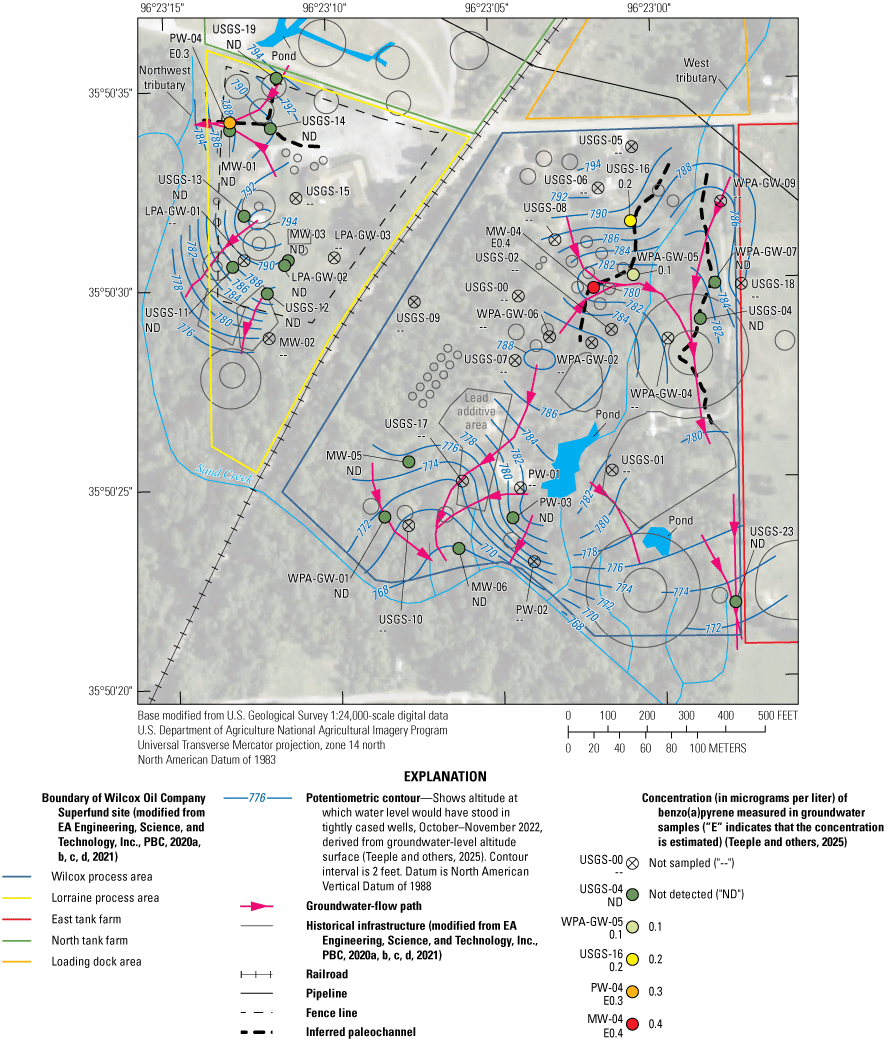
Concentrations of benzo(a)pyrene measured in samples collected from groundwater monitoring wells or piezometers in the Wilcox and Lorraine process areas of the Wilcox Oil Company Superfund site near Bristow, Creek County, Oklahoma, October–November 2022.
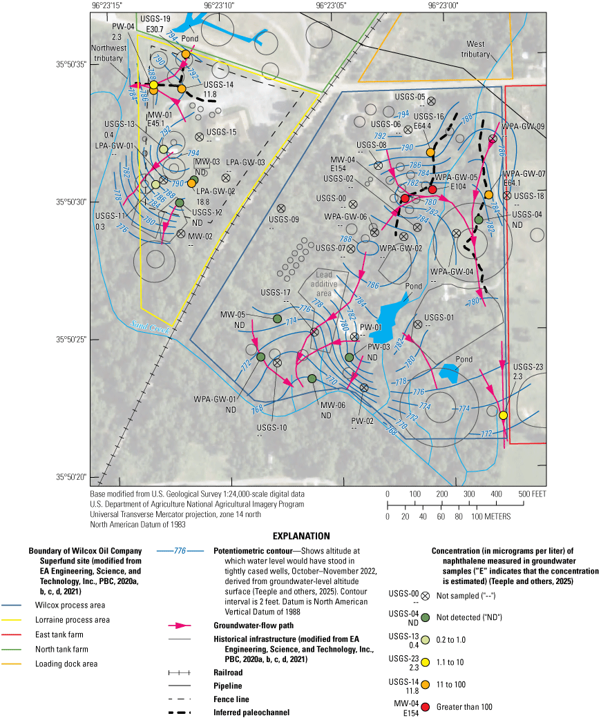
Concentrations of naphthalene measured in samples collected from groundwater monitoring wells or piezometers in the Wilcox and Lorraine process areas of the Wilcox Oil Company Superfund site near Bristow, Creek County, Oklahoma, October–November 2022.
The highest concentrations of SVOCs among the constituents exceeding screening levels were most often measured in samples collected from well MW-04 in the northern part of the Wilcox process area (fig. 2; table 7); high concentrations of selected SVOCs were also measured in the sample collected from well WPA-GW-05 in this same part of the Wilcox process area (fig. 2; table 7). Concentrations of SVOCs are likely the highest in the samples from wells MW-04 and WPA-GW-05 because the direction of groundwater flow (figs. 21 and 22) restricts the migration of contaminants out of the area surrounding these wells. There may be the potential for the contaminants to migrate east and south along the inferred paleochannel that is east of the west tributary to Sand Creek. Because concentrations of SVOCs did not typically exceed screening levels in samples collected from wells outside of the vicinity of well MW-04, results from this sampling event indicate that a plume of substantial areal extent has not developed at the site for SVOCs. There was, however, one well (PW-03) where the groundwater was heavily contaminated with phenol and selected cresol compounds (2-methylphenol; 2,4-dimethylphenol; and 3- and (or) 4-methylphenol) near the southern border of the site; the contaminants in this groundwater have the potential to migrate to Sand Creek along identified groundwater-flow paths.
Trace Elements
Groundwater samples for the analysis of trace elements (including metals) were collected from 25 wells (table 3). Of the 19 trace elements quantified by the analytical methods, 15 were detected in the groundwater samples (table 8). Barium, iron, and manganese were detected in the samples collected from every well. Aluminum was detected in the samples from 22 wells in concentrations ranging from 316 to 122,000 µg/L (fig. 23A). The screening level for aluminum of 20,000 µg/L was exceeded in samples from three wells. Arsenic was detected in the samples from 16 wells at concentrations ranging from 11.8 to 51.9 µg/L (fig. 23B). The screening level of 10 µg/L for arsenic was exceeded in every sample in which it was detected. The screening level of 2,000 µg/L for barium was exceeded in the sample from one well (well WPA-GW-01) (fig. 23C). The screening level of 14,000 µg/L for iron was exceeded in samples from 16 wells (fig. 23D). The screening level of 15 µg/L for lead was exceeded in the samples from 14 wells (fig. 23E). Manganese was detected in the samples from all 25 wells in concentrations ranging from 189 to 7,940 µg/L (fig. 23F). The screening level of 430 µg/L for manganese was exceeded in the samples collected from 20 wells. Although the spatial distribution of trace element concentrations did not follow a specific spatial pattern, the maximum concentrations for 13 of the 15 trace elements detected at the site were measured in the samples from 2 wells: WPA-GW-01, with maximum concentrations for 7 trace elements (aluminum, barium, beryllium, cadmium, iron, manganese, and vanadium), located in the Wilcox process area, and USGS-12, with maximum concentrations for 6 trace elements (chromium, copper, lead, molybdenum, nickel, and zinc), located in the Lorraine process area.
Table 8.
Trace elements detected in groundwater samples collected from groundwater monitoring wells or piezometers in the Wilcox and Lorraine process areas of the Wilcox Oil Company Superfund site near Bristow, Creek County, Oklahoma, October–November 2022.[Data from Teeple and others (2025). µg/L, microgram per liter; ID, identifier; RSL, U.S. Environmental Protection Agency [EPA] Region 6 regional screening level for tapwater (EPA, 2025; EA Engineering, Science, and Technology, Inc., PBC, 2020a); MCL, maximum contaminant level (EPA, 2023b); ─, no data]
| Trace element | Number of detections | Minimum concentration, in µg/L | Maximum concentration, in µg/L | Well ID for well with maximum concentration (figs. 2, 17–22) |
Screening level type | Screening level, in µg/L | Number of times screening level was exceeded |
|---|---|---|---|---|---|---|---|
| Aluminum | 22 | 316 | 122,000 | WPA‑GW‑01 | RSL | 20,000 | 3 |
| Arsenic | 16 | 11.8 | 51.9 | WPA‑GW‑05 | MCL | 10 | 16 |
| Barium | 25 | 78.7 | 2,190 | WPA‑GW‑01 | MCL | 2,000 | 1 |
| Beryllium | 1 | 9.6 | 9.6 | WPA‑GW‑01 | MCL | 4 | 1 |
| Cadmium | 1 | 5.5 | 5.5 | WPA‑GW‑01 | MCL | 5 | 1 |
| Chromium | 13 | 10.2 | 251 | USGS‑12 | MCL | 100 | 2 |
| Cobalt | 4 | 21.1 | 44.9 | WPA‑GW‑01 | None | ─ | ─ |
| Copper | 7 | 26.4 | 1,480 | USGS‑12 | MCL | 1,300 | 1 |
| Iron | 25 | 1,030 | 119,000 | WPA‑GW‑01 | RSL | 14,000 | 16 |
| Lead | 18 | 8.2 | 1,290 | USGS‑12 | MCL | 15 | 15 |
| Manganese | 25 | 189 | 7,940 | WPA‑GW‑01 | RSL | 430 | 21 |
| Molybdenum | 2 | 51.6 | 68.4 | USGS‑12 | None | ─ | ─ |
| Nickel | 15 | 20.8 | 133 | USGS‑12 | RSL | 390 | 0 |
| Vanadium | 8 | 26.0 | 148 | WPA‑GW‑01 | RSL | 86 | 3 |
| Zinc | 22 | 20.3 | 1,400 | USGS‑12 | RSL | 6,000 | 0 |
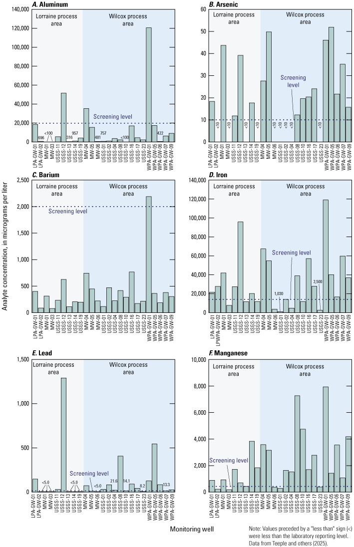
Concentrations of (A) aluminum, (B) arsenic, (C) barium, (D) iron, (E) lead, and (F) manganese measured in samples collected from groundwater monitoring wells or piezometers in the Wilcox and Lorraine process areas of the Wilcox Oil Company Superfund site near Bristow, Creek County, Oklahoma, October–November 2022.
Geochemical and Microbial Indicators of Degradation
Geochemical indicators provide information on the conditions that prevail in an aquifer that are supportive of natural attenuation and help determine if the aquifer has the capacity to naturally degrade contaminants (New Jersey Department of Environmental Protection, 2022). Degradation of organic contaminants in groundwater occurs through oxidation-reduction (redox) reactions facilitated by microorganisms in which electrons are transferred from one compound (the electron donor) to another (the electron acceptor) (New Jersey Department of Environmental Protection, 2022). The primary electron donors in aquifers contaminated as a result of oil refinery operations such as the shallow groundwater system in the Wilcox and Lorraine process areas are organic matter and include petroleum hydrocarbons and other VOCs and SVOCs. Commonly available electron acceptors include iron, manganese, oxygen, nitrate, and sulfate (New Jersey Department of Environmental Protection, 2022; Teeple and others, 2025). The reduction of oxygen generates the maximum amount of available energy; thus, it is used preferentially by oxygen-reducing microorganisms (McMahon and Chapelle, 2008). After oxygen is depleted, the next most energetically favorable available electron acceptor is nitrate, followed by manganese, iron, sulfate, and carbon dioxide (McMahon and Chapelle, 2008). Because of this succession, predominant redox processes tend to be isolated into zones within a contaminant plume. The reduction of these common electron acceptors also produces distinctive compounds that can be monitored in groundwater to assess the redox processes occurring in the groundwater and the potential for degradation of organic contaminants (McMahon and Chapelle, 2008).
pH and ORP, a measure of the relative intensity of oxidizing and reducing conditions in an aquifer, also are geochemical indicators of the relative oxidizing or reducing characteristics of a groundwater system (Hem, 1985). The pH of groundwater can affect the presence and activity of the microbial community. Optimal pH ranges for biodegrading bacteria vary slightly in the literature (for example, from 6.0 to 8.0 standard units [New Jersey Department of Environmental Protection, 2022] and from 5.0 to 9.0 standard units [Corseuil and Alvarez, 1996]) but are typically centered around the neutral pH value of 7.0 standard units (Corseuil and Alvarez, 1996; New Jersey Department of Environmental Protection, 2022). Positive ORP values indicate that the groundwater system is relatively oxidizing, and negative ORP values indicate that it is relatively reducing; thus, it is common to observe lower ORP values within the contaminant plume, where anaerobic biodegradation is occurring, than outside the contaminant plume (Hem, 1985). In addition to geochemical indicators, microbial indicator information such as the identification and quantification of microbial communities can be used to assess potential redox conditions because many redox processes are microbially mediated (Christensen and others, 2000).
Several conditions throughout the site such as groundwater system equilibrium issues, spatial differences in soil contamination, and sampling issues from dewatering wells complicate the determination of redox conditions. Several reduction processes can occur over time because groundwater systems are unlikely to be in thermodynamic equilibrium (Christensen and others, 2000). Redox indicator constituents, such as iron and manganese, from contaminated soil caused by previous activities at the site could be transported into groundwater. There is also more than one area where contamination occurred within the site, limiting the ability to differentiate whether elevated concentrations of redox indicator constituents are a result of contamination from the various sources or from redox processes within the plume. During the sampling event, not all geochemical indicators could be measured at each well because an insufficient volume of water was available for sampling at some wells and because many of the wells that were sampled had been recently installed and thus lacked historical data for assessing temporal trends. These data limitations and confounding factors constrained the ability to fully assess redox conditions at each well; thus, only a general assessment of the potential redox conditions based on geochemical and microbial indicators of degradation is discussed.
In-situ measurements of pH, ORP, and DO were made in 25 wells. pH values ranged from 6.0 to 9.3 standard units (table 9). At 24 wells the pH was within the optimal range for biodegradation of 6 to 8 standard units (New Jersey Department of Environmental Protection, 2022). The only well where the pH was outside this optimal range was well PW-03; the sample from well PW-03 indicated that the groundwater at this well was heavily contaminated with phenol and selected cresol compounds (2-methylphenol; 2,4-dimethylphenol; and 3- and (or) 4-methylphenol) (table 7). ORP values ranged from −209 to 66.5 millivolts for all 25 wells at the site (table 9). A positive ORP value was measured in two of the wells, USGS-04 and USGS-23, whereas a negative ORP value was measured in the remaining wells. Because negative ORP values indicate the presence of a reducing environment appropriate for anaerobic biodegradation (Hem, 1985), the measured ORP values indicate that an environment favorable to anaerobic biodegradation was likely predominant throughout the site. DO concentrations ranged from less than 1.0 to 6.6 milligrams per liter (mg/L) (table 9). Anoxic conditions (DO concentrations less than 1.0 mg/L) were measured in 15 of the 25 wells where DO was measured, indicating that the predominant pathway for degradation is anaerobic. Oxic conditions (DO concentrations greater than or equal to 1.0 mg/L) were measured in seven wells (table 9). Wells WPA-GW-07, USGS-10, and USGS-12 could not be qualified as either oxic or anoxic because these wells dewatered during the sampling process before stabilization of field properties, and their respective DO concentrations of 1.1, 1.8, and 2.0 mg/L were considered estimates. Because the DO concentrations measured in wells WPA-GW-07, USGS-10, and USGS-12 were near the 1.0-mg/L threshold between oxic and anoxic conditions and because field properties were not measured again during the subsequent collection of groundwater-quality samples from these wells, indicators other than DO concentration may be more appropriate for evaluating redox conditions in the groundwater characterized by these wells, such as the prevalence of aerobic and anaerobic bacteria. In the sample from well USGS-12, bacteria of the genus Massilia, which are generally aerobes (Vikram and others, 2017), were the most abundant and represented 56 percent of the total bacterial community, indicating predominantly oxic conditions at this well (Teeple and others, 2025). In the sample from well USGS-10, 53 genera of bacteria were identified; of these 53 genera, at a relative abundance of 14 percent, Massilia was most abundant, followed by Enterobacter, which is facultative anaerobic, at a relative abundance of 11 percent and Geobacter, which is anaerobic but has been found tolerant to oxic conditions (Lin and others, 2004), at a relative abundance of 10 percent (Teeple and others, 2025). In the sample from well USGS-17, a well in which the conditions were oxic, the predominant genera were Geobacter and Pseudomonas, which is facultative anaerobic, at 24 and 15 percent relative abundances, respectively (Teeple and others, 2025). Coexistence of aerobic and anaerobic bacteria in groundwater has been documented (Bekins and others, 1999; Aburto and others, 2009) and indicates that variable redox conditions are likely.
Table 9.
Groundwater geochemical data from samples collected from groundwater monitoring wells or piezometers in the Wilcox and Lorraine process areas of the Wilcox Oil Company Superfund site near Bristow, Creek County, Oklahoma, October–November 2022.[Data from Teeple and others (2025). ID, identifier; DO, dissolved oxygen; mg/L, milligram per liter; µg/L, microgram per liter; ORP, oxidation-reduction potential; mV, millivolt; µS/cm, microsiemens per centimeter; °C, degree Celsius; ─, not sampled; <, less than; >, greater than; E, estimated; w, high variability, questionable precision and accuracy]
| Well ID (figs. 2, 17–22) |
Total iron, in µg/L | Ferrous iron, in µg/L | Total manganese, in µg/L | pH, in standard units | ORP, in mV | DO, in mg/L | Specific conductance, in µS/cm at 25 °C | Temperature, in °C | Nitrate, in mg/L | Nitrite, in mg/L | Sulfate, in mg/L | Sulfide, in mg/L | Methane, in mg/L |
|---|---|---|---|---|---|---|---|---|---|---|---|---|---|
| MW‑01 | 41,900 | >24,000 | 928 | 6.3 | −85.0 | <1.0 | 357 | 21.0 | <0.040 | <0.001 | 0.11 | <0.3 | 5.96 |
| MW‑03 | 7,650 | 5,900 | 189 | 6.3 | −63.9 | 1.0 | 438 | 19.4 | <0.040 | <0.001 | 27.5 | <0.3 | 0.0677 |
| PW‑04 | ─ | ─ | ─ | 6.3 | −104 | <1.0 | 401 | 21.6 | ─ | ─ | ─ | ─ | ─ |
| LPA‑GW‑01 | 21,700 | ─ | 893 | 6.6 | −118 | 1.0 | 886 | 17.8 | ─ | ─ | ─ | ─ | ─ |
| LPA‑GW‑02 | 27,700 | 24,800 | 222 | 6.3 | −68.6 | <1.0 | 377 | 18.6 | <0.040 | <0.001 | 1.15 | <0.3 | 1.54 |
| USGS‑11 | 27,400 | ─ | 1,720 | 6.6 | −116 | <1.0 | 586 | 20.9 | ─ | ─ | ─ | ─ | ─ |
| USGS‑12 | 95,800 | ─ | 690 | 6.0 | −65.9 | E2.0 | 500 | 21.1 | ─ | ─ | ─ | ─ | ─ |
| USGS‑13 | 11,700 | ─ | 438 | 6.7 | −107 | <1.0 | 495 | 22.7 | ─ | ─ | ─ | ─ | ─ |
| USGS‑14 | 20,200 | 17,200 | 3,840 | 6.7 | −104 | <1.0 | 612 | 19.8 | <0.040 | <0.001 | 20.8 | <0.3 | 1.68 |
| USGS‑19 | 11,800 | ─ | 1,840 | 6.7 | −48.6 | w4.8 | 453 | 21.1 | 0.526 | 0.003 | 21.9 | ─ | 0.138 |
| MW‑04 | w67,400 | 2,780 | w3,580 | 6.4 | −102 | <1.0 | 586 | 20.9 | <0.040 | <0.001 | 0.07 | 2.9 | 9.04 |
| MW‑05 | 54,800 | 2,400 | 3,160 | 6.4 | −65.3 | <1.0 | 908 | 21.7 | <0.040 | <0.001 | 64.9 | 1.6 | 0.0101 |
| MW‑06 | 3,600 | 2,600 | 377 | 7.0 | −108 | <1.0 | 895 | 17.7 | <0.040 | <0.001 | 46.8 | <0.3 | 0.0900 |
| PW‑01 | ─ | ─ | ─ | ─ | ─ | ─ | ─ | ─ | <0.040 | 0.001 | 11.1 | ─ | ─ |
| PW‑03 | ─ | ─ | ─ | 9.3 | −209 | <1.0 | 20,200 | 21.0 | ─ | ─ | ─ | ─ | ─ |
| WPA‑GW‑01 | 119,000 | 8,400 | 7,940 | 6.6 | −77.3 | 1.0 | 552 | 23.2 | 0.081 | 0.003 | 0.24 | 1.3 | 0.639 |
| WPA‑GW‑05 | 40,100 | 4,000 | 1,430 | 6.6 | −146 | <1.0 | 1,110 | 19.5 | <0.040 | <0.001 | 0.21 | 1.2 | 11.9 |
| WPA‑GW‑06 | 16,700 | ─ | 3,550 | ─ | ─ | ─ | ─ | ─ | <0.040 | 0.003 | 0.79 | ─ | 1.31 |
| WPA‑GW‑07 | 59,800 | >24,000 | 1,070 | E6.6 | E−107 | E1.1 | E785 | E20.3 | <0.040 | <0.001 | 0.23 | 0.6 | 3.76 |
| WPA‑GW‑09 | 36,900 | ─ | 4,180 | 6.5 | −75.0 | <1.0 | 335 | 25.4 | ─ | ─ | ─ | ─ | ─ |
| USGS‑01 | 1,030 | ─ | 282 | ─ | ─ | ─ | ─ | ─ | ─ | ─ | ─ | ─ | 0.0010 |
| USGS‑02 | 14,000 | ─ | 1,640 | 6.7 | −94.3 | <1.0 | 625 | 21.3 | 0.033 | 0.008 | 83.6 | ─ | ─ |
| USGS‑04 | 4,850 | 2,100 | 1,520 | 6.1 | 66.5 | <1.0 | 486 | 21.9 | <0.040 | 0.001 | 65.7 | ─ | 0.0025 |
| USGS‑08 | 38,900 | ─ | 7,270 | 6.5 | −49.2 | 1.0 | 714 | 21.1 | ─ | ─ | ─ | ─ | 1.79 |
| USGS‑10 | 11,800 | 1,600 | 4,750 | 6.5 | −76.4 | E1.8 | 475 | 19.4 | <0.040 | <0.001 | ─ | <0.3 | 0.674 |
| USGS‑16 | 57,100 | 27,200 | 1,700 | 6.5 | −65.4 | <1.0 | 538 | 18.8 | 0.084 | 0.003 | 4.08 | 5.4 | 4.2 |
| USGS‑17 | 27,800 | ─ | 2,780 | 6.9 | −98.4 | 1.5 | 2,140 | 19.5 | <0.040 | <0.001 | ─ | ─ | 0.220 |
| USGS‑23 | 2,500 | ─ | 382 | 6.8 | 6.9 | 6.6 | 751 | 17.0 | 0.839 | 0.006 | 50.3 | ─ | 0.322 |
Although a DO concentration of 4.8 mg/L was measured at well USGS-19 (table 9), the DO readings during field sampling were highly variable before finally stabilizing, indicating that a potential equipment malfunction could have resulted in an elevated, biased final DO concentration. A DO concentration greater than 1.0 mg/L is also inconsistent with bacterial community data from samples collected at well USGS-19. Results from 16S rRNA analysis indicate that bacteria of the phyla Desulfobacterota and Chloroflexi, which are predominantly anaerobic (Murphy and others, 2021; Yu and others, 2023; Pavlova and others, 2024), represented 61 percent of the total bacterial community at that well (Teeple and others, 2025). At well USGS-23, the highest DO concentration (6.6 mg/L) was recorded among the wells where DO was measured. In the sample from well USGS-23, bacteria of the genus Bacillus, which are predominantly aerobic, were predominant at a 68 percent relative abundance (Teeple and others, 2025). The 6.6 mg/L DO concentration and 68 percent relative abundance of bacteria of the genus Bacillus are indicative of oxic conditions at well USGS-23 (Hu and others, 2022; Yao and others, 2022).
Total iron and ferrous iron were measured in the samples collected from 25 and 13 wells, respectively. Concentrations of total iron ranged from 1,030 to 119,000 µg/L, whereas concentrations of ferrous iron ranged from 1,600 to 27,200 µg/L (table 9). The presence of ferrous iron is an indication of ferric iron reduction during microbial degradation of organic compounds in the absence of oxygen and nitrate (New Jersey Department of Environmental Protection, 2022). In the Wilcox process area, concentrations of total iron were about 2 to 24 times greater than the concentrations of ferrous iron, whereas in the Lorraine process area, the concentrations of total iron were similar to (less than 2 times) the concentrations of ferrous iron. Genera of bacteria that include species capable of reducing iron, such as Aeromonas, Desulfitobacterium, Desulfovibrio, Geobacter, and Hydrogenophaga (Weber and others, 2006), were identified at relative abundances greater than 10 percent in the samples from wells MW-05, WPA-GW-04, USGS-04, USGS-07, USGS-10, USGS-11, USGS-15, and USGS-17 (Teeple and others, 2025). Relative abundances of these genera of bacteria at these wells ranged from 12 to 48 percent. General conditions at the site, including predominantly anoxic conditions, nitrate depletion, and presence of iron-reducing bacteria, are favorable for degradation through iron reduction. These conditions, in combination with high concentrations of ferrous iron at various wells, indicate that iron reduction is likely occurring.
Nitrate was detected at concentrations that ranged from 0.033 to 0.839 mg/L in 5 of the 19 wells that were sampled for this constituent (table 9). The highest concentrations of nitrate were measured in the samples from wells USGS-19 and USGS-23 (0.526 and 0.839 mg/L, respectively). Because oxic conditions were identified at well USGS-23, the nitrate present in the groundwater in and near this well has likely not been depleted, as denitrification is an anaerobic process. If groundwater conditions around well USGS-23 become anoxic, nitrate reduction could occur because bacteria of the genus Bacillus, which are present at high proportions in this well, are capable of reducing nitrate under anoxic conditions (Schirawski and Unden, 1995). Low nitrate concentrations ranging from 0.033 to 0.084 mg/L were measured in the samples collected from the remaining wells in which nitrate was detected. Because nitrate concentrations were low when detected and frequently not detected at all, nitrate reduction at most of the wells is unlikely to be an effective degradation mechanism.
Sulfate was measured in the samples collected from 17 wells at concentrations that ranged from 0.07 to 83.6 mg/L (table 9), with the maximum concentration measured in the sample from well USGS-02. Sulfide was measured in the field at 12 wells, and concentrations ranged from less than 0.3 to 5.4 mg/L. Differentiating between iron reduction and sulfate reduction can be difficult. The concentrations of sulfate measured in the samples from wells MW-03 and USGS-19 or the presence of sulfide in the samples from wells MW-04, MW-05, WPA-GW-01, and USGS-16 in combination with the presence of Desulfobacterota at relative abundances greater than 15 percent at these wells (fig. 24) are indicative of possible sulfate reduction. At wells WPA-GW-04, USGS-10, USGS-11, and USGS-17, sulfate and sulfide were either not measured or not detected in the samples that were collected; however, Desulfobacterota were measured at abundances ranging from 15 to 35 percent at these wells (fig. 24), indicating potential for sulfate reduction. Bacteria of the family Rhodocyclaceae, which includes some species capable of reducing both iron and sulfate, were also present in the samples collected from all wells, with the exception of well MW-03; a high relative abundance (43 percent) of Desulfobacterota was measured in the sample collected from this well (fig. 24).
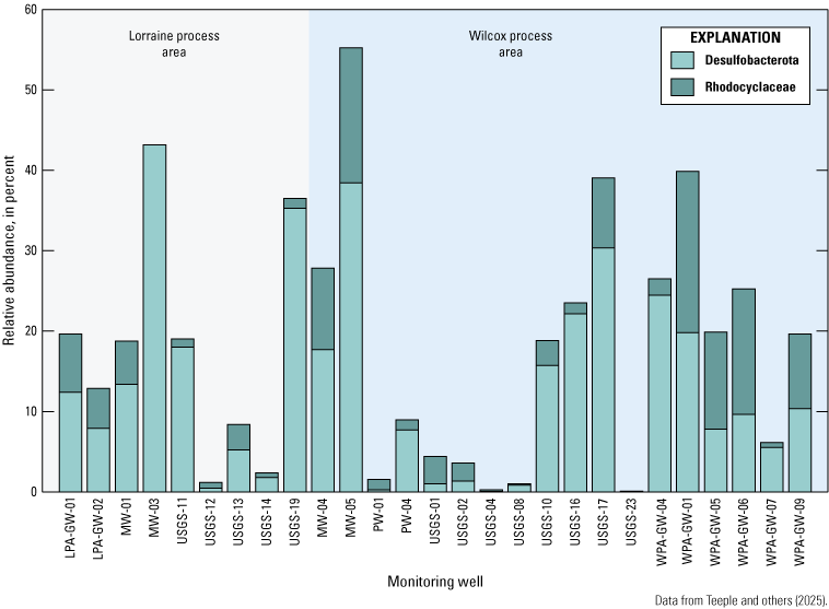
Relative abundance of Desulfobacterota and Rhodocyclaceae measured in samples collected from groundwater monitoring wells or piezometers in the Wilcox and Lorraine process areas of the Wilcox Oil Company Superfund site near Bristow, Creek County, Oklahoma, October–November 2022.
Drinking water standards for methane have not been published; a few observations regarding the concentrations of methane can be made. Methane concentrations ranged from 0.0010 to 11.9 mg/L (table 9). The maximum methane concentration of 11.9 mg/L was measured in a sample collected from well WPA-GW-05, followed by a methane concentration of 9.04 mg/L in the sample from well MW-04, which is near well WPA-GW-05 (fig. 25). Concentrations of methane exceeding 1.00 mg/L were also measured in the samples collected from other wells near well MW-04, such as the samples collected from wells WPA-GW-06, WPA-GW-07, USGS-08, and USGS-16. Other samples exceeding 1.00 mg/L were collected from wells MW-01, LPA-GW-02, and USGS-14 in the Lorraine process area. Methanotrophs of the genera Methylomonas and Methylobacter (Bowman, 2006) were identified in the samples from six wells (MW-03, PW-02, WPA-GW-01, WPA-GW-04, WPA-GW-06, and WPA-GW-09) at relative abundances ranging from 2 to 20 percent; however, the relative abundance of bacteria that were unclassified at the phylum level ranged from 8 to 26 percent in samples with methane concentrations greater than 5.00 mg/L (Teeple and others, 2025). Bacteria of the genus Clostridium and phylum Firmicutes, which includes species capable of participating in acetogenesis (Schuchmann and Müller, 2016), an intermediate step of degradation previous to methanogenesis, were the most abundant in samples with high (greater than 1.00 mg/L) methane concentrations (Teeple and others, 2025).
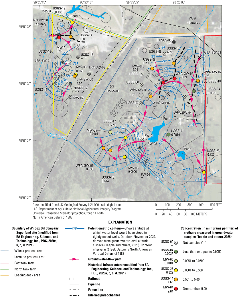
Concentrations of methane measured in samples collected from groundwater monitoring wells or piezometers in the Wilcox and Lorraine process areas of the Wilcox Oil Company Superfund site near Bristow, Creek County, Oklahoma, October–November 2022.
Although the dataset of all the samples available for the determination of redox conditions was relatively small along with limited constituent results because of lacking water for complete sample sets, a general assessment of geochemical and microbial indicators demonstrates that iron, sulfate, and methane reduction processes are likely occurring at the site and could contribute to the natural attenuation of contaminants. In addition, the microbial community identified in the groundwater indicates a potential for bioremediation as iron-, nitrate-, and sulfate-reducing bacteria. Future sampling events that include the collection of samples for measuring dissolved hydrogen concentrations may provide additional data that can help to better determine the predominant redox process in the groundwater at the site (Christensen and others, 2000).
Aquifer Hydraulic Properties
The final hydraulic conductivity values measured in the groundwater monitoring wells screened in the alluvial aquifer at the site ranged from 0.01 to 0.5 ft/d (table 4), resulting in a mean hydraulic conductivity of about 0.2 ft/d. Whereas these hydraulic conductivity values are within the range of hydraulic conductivity values reported in the literature for unconsolidated sediments (3×10⁻⁶ to 8,500 ft/d), they are on the lower end of the range of reported hydraulic conductivity values for clean sands (0.06 to 1,700 ft/d) and exceed the range of reported hydraulic conductivity values of 3×10⁻⁶ to 0.001 ft/d for “fat clays,” which are cohesive and compressible clays of high plasticity (Heath, 1983; Domenico and Schwartz, 1990; American GeoServices, LLC, 2016). The measured hydraulic conductivity values compare reasonably well with the hydraulic conductivity values reported in the technical memorandum on data gap investigation (EA Engineering, Science, and Technology, Inc., PBC, 2020d), which listed values that ranged from 0.07 to 0.64 ft/d. After completion of the slug tests, it was determined that six groundwater monitoring wells (USGS-00, USGS-01, USGS-08, USGS-10, USGS-13, and USGS-17) lacked the pronounced hydraulic connection with the aquifer necessary for unimpeded groundwater movement into and out of the groundwater monitoring well, and therefore, a final hydraulic conductivity value could not be calculated for those groundwater monitoring wells. An estimated range of interstitial velocity values was calculated using the measured range of hydraulic conductivity values, the mean hydraulic gradient the authors of this report estimated at the site (0.04 ft/ft), and an approximate effective porosity value (20 percent) from the EA Engineering, Science, and Technology, Inc., PBC (2020d) report. The estimated range of interstitial velocity values was from 0.002 to 0.1 ft/d (0.7 to 40 ft/yr) with a mean interstitial velocity of 0.04 ft/d (10 ft/yr). These values for the range and mean interstitial velocity vary appreciably from the estimated interstitial velocity of 0.0035 ft/d (1.3 ft/yr) reported in EA Engineering, Science, and Technology, Inc., PBC (2020d); the dissimilarity between these interstitial velocities is a result of the different hydraulic gradient values used in the conversions: 0.04 ft/ft determined in this report compared to 0.002 ft/ft used in EA Engineering, Science, and Technology, Inc., PBC (2020d). Using the same estimated deceleration rate factor for benzene of 2–3 as used in EA Engineering, Science, and Technology, Inc., PBC (2020d), the interstitial velocity for benzene in the groundwater at the site is estimated to be 0.2–20 ft/yr with a mean of about 4 ft/yr.
Summary
The Wilcox Oil Company Superfund site (hereinafter referred to as “the site”) was formerly an oil refinery northeast of Bristow in Creek County, Oklahoma. Crude oil was refined and processed at the site from approximately 1915 to 1963. Products known to have been refined or stored onsite were crude oil, fuel oil, gas oil, distillate, kerosene, naphtha, and benzene (petroleum ether). The Wilcox Oil and Gas Company sold the property in 1963, and from 1975 to 2004, the property was parceled out for residential and commercial development, and a church and seven residences were constructed. Although the site was partially cleared during these transitions, remnants of the former oil refining operations and storage tanks remained as of December 2022.
Historical refinery operations contaminated the soil, surface water, streambed sediments, alluvium, and groundwater with refined and stored products at the site, which led to the property formerly owned by the Wilcox Oil and Gas Company being placed on the National Priorities List on December 12, 2013, and later authorized as a Superfund site when a responsible party for restoration of the site was not identified. Groundwater-quality sampling in 2020 indicated that petroleum hydrocarbons were found in the local shallow perched groundwater system within the alluvium (hereinafter referred to as the “alluvial aquifer”) at the site, but not in the deeper regional groundwater system. The Wilcox and Lorraine process areas are where the highest concentrations of volatile organic compounds (VOCs) (such as benzene), semivolatile organic compounds (SVOCs), polycyclic aromatic hydrocarbons, and trace elements (including metals) (collectively hereinafter referred to as “contaminants”) were measured in the groundwater during previous site assessments. The Wilcox and Lorraine process areas overlie the thickest portions of the alluvium at the site, and understanding the potential migration of contaminants through the soil and groundwater in these areas could help address the areal extent of contamination. Therefore, in 2022, the U.S. Geological Survey (USGS), in cooperation with the U.S. Environmental Protection Agency (EPA), investigated aquifer characteristics of the alluvial aquifer in the Wilcox and Lorraine process areas of the site to fill data gaps related to the geochemistry, nature and extent of contamination, and the fate and transport and the degradation potential of contaminants in the groundwater.
This report documents the results of the groundwater assessment in the Wilcox and Lorraine process areas of the site completed in 2022 by the USGS in cooperation with the EPA. This report (1) documents hydraulic conductivity and other aquifer characteristics of the alluvial aquifer that govern contaminant fate and transport, (2) describes the geospatial extent and concentration of the contaminants in the alluvial aquifer in the Wilcox and Lorraine process areas, and (3) describes the geochemical controls pertaining to oxidation and reduction governing the fate and transport and the degradation potential of contaminants in the groundwater.
Various data were compiled and collected to evaluate the aquifer characteristics at the site including the hydrogeologic framework, groundwater-flow system, geochemistry, and hydraulic properties of the aquifer. A total of 20 new (2022) groundwater monitoring wells were installed at the site to collect data used to supplement groundwater-level altitude and groundwater-quality data collected from older, existing groundwater monitoring wells and piezometers; this combined network of wells is hereinafter referred to as “wells.” Compiled historical soil-core descriptions and depth of refusal information were used in conjunction with collected conductivity logs, soil-core descriptions, and surface geophysical data to characterize the sediments and their extents in the aquifer. Groundwater-level altitude measurements were collected to develop potentiometric-surface maps of the site and to identify potential groundwater-flow direction. Groundwater-quality samples were collected to define the concentration and extent of any contaminants and their byproducts and to estimate natural attenuation potential. Slug tests were completed by the USGS to estimate hydraulic conductivity values at each of the newly installed (2022) groundwater monitoring wells.
The term “hydrogeologic framework” as used in this report refers to the following geologic attributes that govern groundwater flow in the alluvial aquifer: land-surface altitude and orientation, bedrock altitude and orientation, overburden thickness, and sediment characteristics. The land surface and the altitudes to the top of bedrock in the Wilcox and Lorraine process areas generally slope to the south and southwest towards Sand Creek, where the lowest altitudes of the land surface and top of bedrock are along stream channels in the depressions carved by Sand Creek and its west and northwest tributaries. Bedrock is exposed or very near surface to the north of the Wilcox and Lorraine process areas. In the case of the west tributary, the depressions are not located directly below the stream; they are present on either side of the stream. The locations of the depressions likely indicate that the tributary has historically incised what appear to be two paleochannels into the bedrock. The inferred paleochannel to the east of the west tributary has deeper depressions than the inferred paleochannel to the west. Because of the similar slopes between land surface and the top of bedrock, locations with the thickest overburden occur where there are depressions in the bedrock typically related to inferred paleochannels. The primary sediment observed within the overburden consisted of silt to sand-sized unconsolidated sediments that ranged in color from light brown to black. The borehole electrical conductivity logging results were compared to the soil-core descriptions, and there appeared to be three major sediment groups: (1) a clay-dominant group, (2) a sand-dominant group, and (3) a clay and sand mix group. A sand-dominant group thickness within the overburden of less than or equal to 10 feet (ft) was evident in most (about 90 percent) of the gridded area. A comparatively thick sand-dominant group (greater than 15 ft thick in some areas) was mapped in the bedrock east of the west tributary to Sand Creek; this comparatively thick sand-dominant group coincides with the location of an inferred paleochannel. Evaluating the mean normalized resistivity values for the sand-dominant parts of the overburden can potentially identify areas that contain a higher percentage of sand and gravel compared to fine-grained sediments. In about 75 percent of the gridded area, the mean normalized resistivity values in the sand-dominant group were interpreted as being less than 210 ohm-meters (ohm-m). Areas with mean normalized resistivity values greater than 210 ohm-m in the sand-dominant group thickness are generally associated with areas of thin overburden. These high mean normalized resistivity values may indicate that the bedrock in these locations consists of exposed sandstone layers as opposed to the upper mudstone unit of the Paleozoic-age (Upper Pennsylvanian Period) Barnsdall Formation; weathering of the interbedded layers of sandstone found in the Barnsdall Formation has likely resulted in an abundance of sandstone gravel and sand in these areas. In the northeastern part of the Wilcox process area, some of this weathered sandstone may have filled in paleochannels on either side of the west tributary.
Potentiometric-surface maps were created from the groundwater-level altitude data collected prior to the collection of groundwater-quality samples during October–November 2022 to help assess spatial changes in groundwater-level altitudes across the study area. Groundwater-level altitudes in the alluvial aquifer in the Wilcox and Lorraine process areas are affected by the overburden and bedrock altitudes. With such a thin overburden in the area, the presence of groundwater and the groundwater flow in the alluvial aquifer are highly dependent on the bedrock altitude. During October–November 2022, groundwater was absent in the north-central part of the Wilcox and Lorraine process areas because the bedrock altitudes were higher than the groundwater-level altitudes in these parts. In general, groundwater flows south towards Sand Creek, although bedrock highs in the Wilcox and Lorraine process areas affect the flow of groundwater at more localized scales. In the Wilcox process area, there is a bedrock high in the central part of the process area that acts as a groundwater divide, causing groundwater to flow in opposite directions on either side of this high. Groundwater to the north of this divide flows east and then south, following the location of an inferred paleochannel east from the west tributary to Sand Creek in the south. Similar to the Wilcox process area, there is a bedrock high in the central part of the Lorraine process area that acts as a groundwater divide. Groundwater north of this divide follows separate flow paths that join and flow west towards the northwest tributary. Base on the groundwater-level altitudes measured during October–November 2022, the mean groundwater gradient for the Wilcox and Lorraine process areas is 0.04 foot per foot.
Groundwater-quality samples were collected from 33 wells during October–November 2022. Samples were collected and shipped for laboratory analysis of VOCs, SVOCs, trace elements (including metals), major ions, natural attenuation parameters, and natural attenuation biomarkers. Wells that were coincident with or proximal to bedrock highs (MW-02, LPA-GW-03, USGS-00, USGS-05, USGS-09, and USGS-15) were not sampled because they contained insufficient water. For the wells that were sampled, groundwater results for VOCs, SVOCs, and trace elements were compared against screening levels established for the site by the EPA. Groundwater samples for the analysis of VOCs were collected from 29 wells, of which VOCs were detected in the samples from 26 of these wells, and the number of VOCs detected in the samples from a given well ranged from 1 to 8. Of the 49 VOCs quantified, the concentrations of 6 VOCs exceeded their respective screening levels in samples collected from 1 or more wells. SVOCs were detected in the samples from 17 of the 19 wells that were sampled, and the number of SVOCs detected in the samples from a given well ranged from 1 to 18. Of the 70 constituents quantified by the analytical methods, 25 were detected in groundwater samples collected at the site. The highest concentrations of VOCs and SVOCs among the constituents exceeding screening levels were most often measured in samples collected from well MW-04 in the northern part of the Wilcox process area; high concentrations of selected VOCs and SVOCs were also measured in the sample collected from well WPA-GW-05 in this same part of the Wilcox process area. Periodic releases of contaminants into the soil in the Wilcox process area likely resulted in migration of these contaminants into the groundwater. Because of the direction of groundwater flow, contaminants are likely to remain in the area surrounding well MW-04 with perhaps the potential to migrate east and to the south along the inferred paleochannel east of the west tributary to Sand Creek. Because concentrations of VOCs and SVOCs did not typically exceed screening levels at wells outside of the vicinity of MW-04, results from this sampling event indicate that a plume of substantial areal extent has not developed at the site for VOCs and SVOCs. There was, however, one well (PW-03) where the groundwater was heavily contaminated with phenol and selected cresol compounds (2-methylphenol; 2,4-dimethylphenol; and 3- and (or) 4-methylphenol) near the southern border of the site; the contaminants in this groundwater have the potential to migrate to Sand Creek along identified groundwater-flow paths. Groundwater samples for the analysis of trace elements (including metals) were collected from 25 wells. Of the 19 trace elements quantified by the analytical methods, 15 were detected in the groundwater samples. Although the spatial distribution of trace element concentrations did not follow a specific spatial pattern, the maximum concentrations for 13 of the 15 trace elements detected at the site were measured in the samples from 2 wells: WPA-GW-01, with maximum concentrations for 7 trace elements (aluminum, barium, beryllium, cadmium, iron, manganese, and vanadium), located in the Wilcox process area, and USGS-12, with maximum concentrations for 6 trace elements (chromium, copper, lead, molybdenum, nickel, and zinc), located in the Lorraine process area.
Geochemical indicators provide information on the conditions that prevail in an aquifer that are supportive of natural attenuation and help determine if the aquifer has the capacity to naturally degrade contaminants. Several conditions throughout the site such as groundwater system equilibrium issues, spatial differences in soil contamination, and sampling issues from dewatering wells complicate the determination of oxidation-reduction (redox) conditions. These data limitations and confounding factors constrained the ability to fully assess redox conditions at each well; thus, only a general assessment of the potential redox conditions based on geochemical and microbial indicators of degradation is discussed. In-situ measurements of pH, oxidation-reduction potential (ORP), and dissolved oxygen (DO) were made in 25 wells. At 24 wells the pH was within the optimal range for biodegradation of 6 to 8 standard units. A positive ORP value was measured in two of the wells, USGS-04 and USGS-23, whereas a negative ORP value was measured in the remaining wells, indicating that an environment favorable to anaerobic biodegradation was likely predominant throughout the site. Anoxic conditions (DO concentrations less than 1.0 milligram per liter [mg/L]) were measured in 15 of the 25 wells where DO was measured, indicating that the predominant pathway for degradation is anaerobic. Total iron and ferrous iron were measured in the samples collected from 25 and 13 wells, respectively. Concentrations of total iron ranged from 1,030 to 119,000 micrograms per liter (µg/L), whereas concentrations of ferrous iron ranged from 1,600 to 27,200 µg/L. Nitrate was detected at concentrations that ranged from 0.033 to 0.839 mg/L in 5 of the 19 wells that were sampled for this constituent. The highest concentrations of nitrate were measured in the samples from wells USGS-19 and USGS-23 (0.526 and 0.839 mg/L, respectively). Sulfate was measured in the samples collected from 17 wells at concentrations that ranged from 0.07 to 83.6 mg/L, with the maximum concentration measured in the sample from well USGS-02. Sulfide was measured in the field at 12 wells, and concentrations ranged from less than 0.3 to 5.4 mg/L. Methane concentrations ranged from 0.0010 to 11.9 mg/L. Concentrations of methane exceeding 1.00 mg/L were measured in the samples collected from other wells near well MW-04, such as the samples collected from wells WPA-GW-06, WPA-GW-07, USGS-08, and USGS-16. Other samples with concentrations exceeding 1.00 mg/L were collected from wells MW-01, LPA-GW-02, and USGS-14 in the Lorraine process area. Although the dataset of all samples available for the determination of redox conditions was relatively small along with limited constituent results because of lacking water for complete sample sets, a general assessment of geochemical and microbial indicators demonstrates that iron, sulfate, and methane reduction processes are likely occurring at the site and could contribute to the natural attenuation of contaminants. In addition, the microbial community identified in the groundwater indicates a potential for bioremediation as iron-, nitrate-, and sulfate-reducing bacteria.
In November and December 2022, following groundwater monitoring well development and groundwater-quality sampling, slug tests were completed on each of the groundwater monitoring wells installed in 2022 to (1) determine if the wells were in good hydraulic connection with the aquifer and (2) estimate the hydraulic conductivity of the aquifer at each well. After completion of the slug tests, it was determined that six groundwater monitoring wells (USGS-00, USGS-01, USGS-08, USGS-10, USGS-13, and USGS-17) lacked the pronounced hydraulic connection with the aquifer necessary for unimpeded groundwater movement into and out of the groundwater monitoring well, and therefore, a final hydraulic conductivity value could not be calculated for those groundwater monitoring wells. The final hydraulic conductivity values measured in the groundwater monitoring wells screened in the alluvial aquifer at the site ranged from 0.01 to 0.5 foot per day (ft/d), resulting in a mean hydraulic conductivity of about 0.2 ft/d. The estimated range of interstitial velocity values was from 0.002 to 0.1 ft/d (0.7 to 40 feet per year [ft/yr]) with a mean interstitial velocity of 0.04 ft/d (10 ft/yr). Using an estimated deceleration rate factor for benzene of 2–3, the interstitial velocity for benzene in the groundwater at the site is estimated to be 0.2–20 ft/yr with a mean of about 4 ft/yr.
References Cited
Abraham, J.D., Deszcz-Pan, M., Fitterman, D.V., and Burton, B.L., 2006, Use of a handheld broadband EM induction system for deriving resistivity depth images, in EEGS Symposium on the Application of Geophysics to Engineering and Environmental Problems (SAGEEP), 19th, Seattle, Wash., April 2–6, 2006, [Proceedings]: European Association of Geoscientists & Engineers, 18 p., accessed August 22, 2023, at https://doi.org/10.3997/2214-4609-pdb.181.181.
Aburto, A., Fahy, A., Coulon, F., Lethbridge, G., Timmis, K.N., Ball, A.S., and McGenity, T.J., 2009, Mixed aerobic and anaerobic microbial communities in benzene‐contaminated groundwater: Journal of Applied Microbiology, v. 106, no. 1, p. 317–328, accessed May 19, 2023, at https://doi.org/10.1111/j.1365-2672.2008.04005.x.
Advanced Geosciences, Inc., 2009, Instruction manual for EarthImager 2D—Resistivity and IP inversion software (ver. 2.4.0): Advanced Geosciences, Inc., accessed April 3, 2025, at http://www.advancedgeosciences.com/files/eicust/EarthImager2DManual.zip.
American GeoServices, LLC, 2016, Fat clays: American GeoServices, LLC, web page, accessed July 10, 2024, at https://americangeoservices.com/fat-clays.html#:~:text=What%20are%20Fat%20Clays%3F,are%20especially%20attractive%20to%20water.
Ball, L.B., Kress, W.H., Steele, G.V., Cannia, J.C., and Andersen, M.J., 2006, Determination of canal leakage potential using continuous resistivity profiling techniques, Interstate and Tri-State Canals, western Nebraska and eastern Wyoming, 2004: U.S. Geological Survey Scientific Investigations Report 2006–5032, 53 p., accessed June 9, 2022, at https://doi.org/10.3133/sir20065032.
Bekins, B.A., Godsy, E.M., and Warren, E., 1999, Distribution of microbial physiologic types in an aquifer contaminated by crude oil: Microbial Ecology, v. 37, no. 4, p. 263–275, accessed May 19, 2023, at https://doi.org/10.1007/s002489900149.
Bouwer, H., and Rice, R.C., 1976, A slug test for determining hydraulic conductivity of unconfined aquifers with completely or partially penetrating wells: Water Resources Research, v. 12, no. 3, p. 423–428, accessed May 25, 2023, at https://doi.org/10.1029/WR012i003p00423.
Bowman, J., 2006, The methanotrophs—The families Methylococcaceae and Methylocystaceae, in Dworkin, M., Falkow, S., Rosenberg, E., Schleifer, K.H., and Stackebrandt, E., eds., The prokaryotes: New York, Springer, p. 266–289, accessed July 12, 2024, at https://doi.org/10.1007/0-387-30745-1_15.
Burgess Engineering and Testing, Inc., 2010, Report of pedological soil survey for U.S. Highway 77 improvements south of Tonkawa, Kay County, Oklahoma: Smith Roberts Baldischwiler, LLC, prepared by Burgess Engineering and Testing, Inc., Moore, Oklahoma, project no. SSP–136C(101)SS, State job no. 21854(04), BETI project no. 731–10119, 129 p., accessed June 24, 2024, at https://www.odot.org/contracts/a2013/docs1309/CO240_091913_JP2185404_Geotech.pdf.
Burton, B.L., Powers, M.H., and Ball, L.B., 2014, Characterization of subsurface stratigraphy along the lower American River floodplain using electrical resistivity, Sacramento, California, 2011: U.S. Geological Survey Open-File Report 2014–1242, 62 p., accessed June 9, 2022, at https://doi.org/10.3133/ofr20141242.
Center for International Earth Science Information Network [CIESIN] Columbia University, 2023, Gridded population of the world, version 4 (GPWv4)—Population count, revision 11: Palisades, New York, National Aeronautics and Space Administration Socioeconomic Data and Applications Center (SEDAC), accessed April 3, 2025, at https://doi.org/10.7927/H49C6VHW.
CHEMetrics, 2023, Instrumental colorimetric analysis—The Vacu-vials method: CHEMetrics web page, accessed April 28, 2023, at https://www.chemetrics.com/instrumental/.
Christensen, T.H., Bjerg, P.L., Banwart, S.A., Jakobsen, R., Heron, G., and Albrechtsen, H.J., 2000, Characterization of redox conditions in groundwater contaminant plumes: Journal of Contaminant Hydrology, v. 45, nos. 3–4, p. 165–241, accessed May 19, 2023, at https://doi.org/10.1016/S0169-7722(00)00109-1.
Corseuil, H.X., and Alvarez, P.J., 1996, Natural bioremediation perspective for BTX-contaminated groundwater in Brazil—Effect of ethanol: Water Science and Technology, v. 34, nos. 7–8, p. 311–318, accessed August 22, 2023, at https://doi.org/10.2166/wst.1996.0636.
Cunningham, W.L., and Schalk, C.W., 2011, Groundwater technical procedures of the U.S. Geological Survey: U.S. Geological Survey Techniques and Methods, book 1, chap. A1, 151 p., accessed March 11, 2022, at https://doi.org/10.3133/tm1A1.
EA Engineering, Science, and Technology, Inc., PBC, 2016, Sampling and analysis plan—Remedial investigation/feasibility study; Wilcox Oil Company Superfund site; Bristow, Creek County, Oklahoma: U.S. Environmental Protection Agency, Region 6, prepared by EA Engineering, Science, and Technology, Inc., PBC, Lewisville, Texas, under contract no. EP–W–06–004, EPA identification no. OK0001010917, 736 p., accessed June 21, 2024, at https://semspub.epa.gov/work/06/500023340.pdf.
EA Engineering, Science, and Technology, Inc., PBC, 2019, Final remedial design report for source control; Wilcox Oil Company Superfund site; Bristow, Creek County, Oklahoma: U.S. Environmental Protection Agency, Region 6, prepared by EA Engineering, Science, and Technology, Inc., PBC, Lewisville, Texas, under contract no. EP–W–06–004, EPA identification no. OK0001010917, 169 p., accessed May 30, 2023, at https://semspub.epa.gov/work/06/100017609.pdf.
EA Engineering, Science, and Technology, Inc., PBC, 2020a, Remedial investigation report; Wilcox Oil Company Superfund site; Bristow, Creek County, Oklahoma (revision 02): U.S. Environmental Protection Agency, Region 6, prepared by EA Engineering, Science, and Technology, Inc., PBC, Lewisville, Texas, under contract no. EP–W–06–004, EPA identification no. OK0001010917, 3,242 p., accessed May 31, 2022, at https://semspub.epa.gov/work/06/90043353.pdf.
EA Engineering, Science, and Technology, Inc., PBC, 2020b, Human health risk assessment—Remedial investigation/feasibility study; Wilcox Oil Company Superfund site; Bristow, Creek County, Oklahoma: U.S. Environmental Protection Agency, Region 6, prepared by EA Engineering, Science, and Technology, Inc., PBC, Lewisville, Texas, under contract no. EP–W–06–004, EPA identification no. OK0001010917, 895 p., accessed May 31, 2022, at https://semspub.epa.gov/work/06/100022980.pdf.
EA Engineering, Science, and Technology, Inc., PBC, 2020c, Screening level ecological risk assessment—Remedial investigation/feasibility study; Wilcox Oil Company Superfund site; Bristow, Creek County, Oklahoma: U.S. Environmental Protection Agency, Region 6, prepared by EA Engineering, Science, and Technology, Inc., PBC, Lewisville, Texas, under contract no. EP–W–06–004, EPA identification no. OK0001010917, 373 p., accessed May 31, 2022, at https://semspub.epa.gov/work/06/100022981.pdf.
EA Engineering, Science, and Technology, Inc., PBC, 2020d, Technical memorandum on data gap investigation, app. B in Soil feasibility study report—Remedial investigation/feasibility study; Wilcox Oil Company Superfund site; Bristow, Creek County, Oklahoma: U.S. Environmental Protection Agency, Region 6, prepared by EA Engineering, Science, and Technology, Inc., PBC, Lewisville, Texas, under contract no. EP–W–06–004, EPA identification no. OK0001010917, p. 83–3,155, accessed April 12, 2022, at https://semspub.epa.gov/work/06/90044670.pdf.
EA Engineering, Science, and Technology, Inc., PBC, 2021, Soil feasibility study report—Remedial investigation/feasibility study; Wilcox Oil Company Superfund site; Bristow, Creek County, Oklahoma: U.S. Environmental Protection Agency, Region 6, prepared by EA Engineering, Science, and Technology, Inc., PBC, Lewisville, Texas, under contract no. EP–W–06–004, EPA identification no. OK0001010917, 2,923 p., accessed April 12, 2022, at https://semspub.epa.gov/work/06/90044670.pdf.
Ecology and Environment, Inc., 1999, Site assessment report for Wilcox Refinery, Bristow, Creek County, Oklahoma: U.S. Environmental Protection Agency, Region 6, prepared by Ecology and Environment, Inc., Dallas, Texas, under contract no. 68–W6–0013, 2,006 p., accessed May 30, 2023, at https://semspub.epa.gov/work/06/9095400.pdf.
Fishman, M.J., and Friedman, L.C., eds., 1989, Methods for determination of inorganic substances in water and fluvial sediments: U.S. Geological Survey Techniques of Water-Resources Investigations, book 5, chap. A1, 545 p., accessed February 9, 2023, at https://doi.org/10.3133/twri05A1.
Fitterman, D.V., and Labson, V.F., 2005, Electromagnetic induction methods for environmental problems, chap. 10 in Butler, D.K., ed., Near-surface geophysics—Part 1, concepts and fundamentals: Tulsa, Oklahoma, Society of Exploration Geophysics, p. 301–356, accessed August 22, 2023, at https://doi.org/10.1190/1.9781560801719.ch10.
Geophex, Ltd., 2024, GEM-2—How it works—Detailed: Geophex, Ltd., web page, accessed July 10, 2024, at https://geophex.com/gem-2-how-it-works-detailed/.
Hach, 2023, Hach—2100Q portable turbidimeter: Hach web page, accessed January 19, 2023, at https://www.hach.com/p-2100q-portable-turbidimeter/2100Q01.
Heath, R.C., 1983, Basic ground-water hydrology: U.S. Geological Survey Water-Supply Paper 2220, 86 p., accessed May 25, 2023, at https://doi.org/10.3133/wsp2220.
Hem, J.D., 1985, Study and interpretation of the chemical characteristics of natural water: U.S. Geological Survey Water-Supply Paper 2254, 272 p., accessed August 22, 2023, at https://doi.org/10.3133/wsp2254.
Hu, D., Wu, J., Fan, L., Li, S., and Jia, R., 2022, Aerobic degradation characteristics and mechanism of decabromodiphenyl ether (BDE-209) using complex bacteria communities: International Journal of Environmental Research and Public Health, v. 19, no. 24, article 17012, accessed July 12, 2024, at https://doi.org/10.3390/ijerph192417012.
Huang, H., and Won, I.J., 2000, Conductivity and susceptibility mapping using broadband electromagnetic sensors: Journal of Environmental & Engineering Geophysics, v. 5, no. 4, p. 31–41, accessed August 22, 2023, at https://doi.org/10.4133/JEEG5.4.31.
Hudson, F., 2004, Sample preparation and calculations for dissolved gas analysis in water samples using a GC headspace equilibration technique (revision no. 2): U.S. Environmental Protection Agency, RSKSOP–175, 15 p., accessed February 9, 2023, at https://archive.epa.gov/region1/info/testmethods/web/pdf/rsksop175v2.pdf.
In-Situ Inc., 2023a, In-Situ—Aqua TROLL 600 multiparameter sonde: In-Situ Inc., web page, accessed January 19, 2023, at https://in-situ.com/us/aqua-troll-600-multiparameter-sonde.
In-Situ Inc., 2023b, In-Situ—Level TROLL 500 data logger: In-Situ Inc., web page, accessed May 26, 2023, at https://in-situ.com/us/level-troll-500-data-logger.
Kejr, Inc., 2023a, Direct push tooling: Geoprobe Systems web page, accessed May 24, 2023, at https://geoprobe.com/tooling/direct-push-tooling.
Kejr, Inc., 2023b, Direct push drill rigs: Geoprobe Systems web page, accessed May 25, 2023, at https://geoprobe.com/drilling-rigs/direct-push-drill-rigs.
Kejr, Inc., 2023c, EC—Electrical conductivity: Geoprobe Systems web page, accessed May 25, 2023, at https://geoprobe.com/direct-image/ec-electrical-conductivity.
Kejr, Inc., 2023d, Prepacked screen monitoring wells: Geoprobe Systems web page, accessed May 25, 2023, at https://geoprobe.com/tooling/prepacked-screen-monitoring-wells.
Kottek, M., Grieser, J., Beck, C., Rudolf, B., and Rubel, F., 2006, World map of the Köppen-Geiger climate classification updated: Meteorologische Zeitschrift, v. 15, no. 3, p. 259–263, accessed August 22, 2023, at https://doi.org/10.1127/0941-2948/2006/0130.
Kozich, J.J., Westcott, S.L., Baxter, N.T., Highlander, S.K., and Schloss, P.D., 2013, Development of a dual-index sequencing strategy and curation pipeline for analyzing amplicon sequence data on the MiSeq Illumina sequencing platform: Applied and Environmental Microbiology, v. 79, no. 17, p. 5112–5120, accessed June 21, 2023, at https://doi.org/10.1128/AEM.01043-13.
Lin, W.C., Coppi, M.V., and Lovley, D.R., 2004, Geobacter sulfurreducens can grow with oxygen as a terminal electron acceptor: Applied and Environmental Microbiology, v. 70, no. 4, p. 2525–2528, accessed May 19, 2023, at https://doi.org/10.1128/AEM.70.4.2525-2528.2004.
Lockheed Martin Scientific, Engineering, Response and Analytical Services [Lockheed Martin SERAS], 2016, Wilcox Oil Company Superfund site trip report—November 30, 2015 through December 16, 2015: Environmental Protection Agency/Environmental Response Team, prepared by Lockheed Martin Scientific, Engineering, Response and Analytical Services, Edison, New Jersey, document no. SERAS0277–DTR–060216, 23 p., accessed April 12, 2022, at https://semspub.epa.gov/work/06/500022770.pdf.
Loke, M.H., 2004, Tutorial—2-D and 3-D electrical imaging surveys [Geotomo software]: Edmonton, Canada, University of Alberta, 128 p., accessed July 10, 2024, at https://sites.ualberta.ca/~unsworth/UA-classes/223/loke_course_notes.pdf.
Lucius, J.E., Langer, W.H., and Ellefsen, K.J., 2007, An introduction to using surface geophysics to characterize sand and gravel deposits: U.S. Geological Survey Circular 1310, 33 p., accessed August 22, 2023, at https://doi.org/10.3133/cir1310.
McMahon, P.B., and Chapelle, F.H., 2008, Redox processes and water quality of selected principal aquifer systems: Ground Water, v. 46, no. 2, p. 259–271, accessed August 22, 2023, at https://doi.org/10.1111/j.1745-6584.2007.00385.x.
Minnesota Pollution Control Agency, 2023, Minnesota stormwater manual—Understanding and interpreting soils and soil boring reports for infiltration BMPs: Minnesota Pollution Control Agency web page, accessed July 10, 2024, at https://stormwater.pca.state.mn.us/index.php/Understanding_and_interpreting_soils_and_soil_boring_reports_for_infiltration_BMPs.
Munsell Color Co., Inc., 1992, Munsell soil color charts (revised ed.): Grand Rapids, Michigan, Munsell Color Co., Inc., [leaves, unnumbered]. [Also available at https://munsell.com/color-products/color-communications-products/environmental-color-communication/munsell-soil-color-charts/.]
Murphy, C.L., Biggerstaff, J., Eichhorn, A., Ewing, E., Shahan, R., Soriano, D., Stewart, S., VanMol, K., Walker, R., Walters, P., Elshahed, M.S., and Youssef, N., 2021, Genomic characterization of three novel Desulfobacterota classes expand the metabolic and phylogenetic diversity of the Phylum: Environmental Microbiology, v. 23, no. 8, p. 4,326–4,343, accessed April 2, 2025, at https://doi.org/10.1111/1462-2920.15614.
National Weather Service, 2023, Bristow climatology: National Weather Service web page, accessed May 23, 2023, at https://www.weather.gov/tsa/climo_bristow.
Natural Resources Conservation Service, 2019, Soil Survey Geographic Database (SSURGO)—Creek County, Oklahoma: Fort Worth, Texas, U.S. Department of Agriculture Natural Resources Conservation Service database, accessed May 30, 2023, at https://websoilsurvey.sc.egov.usda.gov/.
New Jersey Department of Environmental Protection, 2022, Monitored natural attenuation technical guidance version 2.0: Contaminated Site Remediation & Redevelopment Program, 53 p., accessed March 20, 2025, at https://dep.nj.gov/wp-content/uploads/srp/mna_guidance.pdf?v_2.
Oklahoma Department of Environmental Quality, 1994, Preliminary assessment of the Wilcox Oil Company located in Bristow, Creek County, Oklahoma: U.S. Environmental Protection Agency, prepared by State of Oklahoma Department of Environmental Quality, 561 p., accessed May 30, 2023, at https://semspub.epa.gov/work/06/698560.pdf.
Oklahoma Department of Environmental Quality, 2008, Preliminary assessment of the Lorraine Refinery site located near Bristow, Creek County, Oklahoma: U.S. Environmental Protection Agency, prepared by State of Oklahoma Department of Environmental Quality, 153 p., accessed May 30, 2023, at https://semspub.epa.gov/work/06/698566.pdf.
Oklahoma Department of Environmental Quality, 2009, Site inspection of the Lorraine Refinery (Lorraine Refining Company), Creek County, Oklahoma: U.S. Environmental Protection Agency, prepared by State of Oklahoma Department of Environmental Quality, 276 p., accessed May 30, 2023, at https://semspub.epa.gov/work/06/874466.pdf.
Oklahoma Department of Environmental Quality, 2010, Expanded site inspection report, Lorraine Refinery, Creek County, Oklahoma: U.S. Environmental Protection Agency, prepared by State of Oklahoma Department of Environmental Quality, 336 p., accessed May 30, 2023, at https://semspub.epa.gov/work/06/698539.pdf.
Oklahoma Department of Environmental Quality, 2011, Expanded site inspection report, Wilcox Refinery, Creek County, Oklahoma: U.S. Environmental Protection Agency, prepared by State of Oklahoma Department of Environmental Quality, 432 p., accessed May 30, 2023, at https://semspub.epa.gov/work/06/698541.pdf.
Oklahoma Department of Environmental Quality, 2016, Memo—Radiation survey, Wilcox Oil Company Superfund site: Oklahoma Department of Environmental Quality, 1 p., accessed May 30, 2023, at https://semspub.epa.gov/work/06/500025090.pdf.
Osborn, N.I., and Hardy, R.H., 1999, Statewide groundwater vulnerability map of Oklahoma: Oklahoma Water Resources Board Technical Report 99–1, 34 p., accessed August 4, 2023, at https://www.owrb.ok.gov/studies/reports/gwvulnerability/entire-report.pdf.
Patton, C.J., and Kryskalla, J.R., 2011, Colorimetric determination of nitrate plus nitrite in water by enzymatic reduction, automated discrete analyzer methods: U.S. Geological Survey Techniques and Methods, book 5, chap. B8, 34 p., accessed February 9, 2023, at https://doi.org/10.3133/tm5B8.
Pavlova, O.N., Bukin, S.V., Izosimova, O.N., Chernitsina, S.M., Ivanov, V.G., Khabuev, A.V., Pogodaeva, T.V., Elovskaya, I.S., Gorshkov, A.G., and Zemskaya, T.I., 2024, Anaerobic oxidation of oil by microbial communities of bottom sediments of a natural oil seepage site (Bolshaya Zelenovskaya, Middle Baikal): Microbiology, v. 93, p. 563–575, accessed April 2, 2025, at https://doi.org/10.1134/S0026261724605608.
Pettijohn, F.J., Potter, P.E., and Siever, R., 1973, Sand and sandstones: New York, Springer-Verlag, 583 p., accessed June 24, 2024, at https://doi.org/10.1007/978-1-4615-9974-6.
Poppe, L.J., McMullen, K.Y., Williams, S.J., and Paskevich, V.F., eds., 2005, USGS east-coast sediment analysis—Procedures, database, and GIS data (ver. 3.0, November 2014): U.S. Geological Survey Open-File Report 2005–1001, accessed October 30, 2024, at https://doi.org/10.3133/ofr20051001.
Puls, R.W., and Barcelona, M.J., 1996, Low-flow (minimal drawdown) ground-water sampling procedures: U.S. Environmental Protection Agency, EPA/540/S–95/504, 12 p., accessed January 19, 2023, at https://www.epa.gov/sites/default/files/2015-06/documents/lwflw2a.pdf.
Quast, C., Pruesse, E., Yilmaz, P., Gerken, J., Schweer, T., Yarza, P., Peplies, J., and Glöckner, F.O., 2012, The SILVA ribosomal RNA gene database project—Improved data processing and web-based tools: Nucleic Acids Research, v. 41, no. D1, p. D590–D596, accessed June 21, 2023, at https://doi.org/10.1093/nar/gks1219.
Roy F. Weston, Inc., 1997, Expanded site inspection report—Wilcox Oil Company; Bristow, Creek County, OK: U.S. Environmental Protection Agency, Region 6, prepared by Roy F. Weston, Inc., Houston, Texas, under contract no. 68–W9–0015, 555 p., accessed May 30, 2023, at https://semspub.epa.gov/work/06/698550.pdf.
S2C2, Inc., 2016, Data analysis and data visualization for the Wilcox Refinery Superfund site, Bristow, Oklahoma: Lockheed Martin/SERAS, prepared by S2C2, Inc., Flemington, New Jersey, document no. SERAS0277–DTR–060216, 469 p., accessed April 12, 2022, at https://semspub.epa.gov/work/06/500022770.pdf.
Schirawski, J., and Unden, G., 1995, Anaerobic respiration of Bacillus macerans with fumarate, TMAO, nitrate and nitrite and regulation of the pathways by oxygen and nitrate: Archives of Microbiology, v. 163, no. 2, p. 148–154, accessed May 19, 2023, at https://doi.org/10.1007/BF00381790.
Schlee, J., 1973, Atlantic continental shelf and slope of the United States—Sediment texture of the northeastern part: U.S. Geological Survey Professional Paper 529–L, 64 p., 6 pls., accessed October 30, 2024, at https://doi.org/10.3133/pp529L.
Schloss, P.D., Westcott, S.L., Ryabin, T., Hall, J.R., Hartmann, M., Hollister, E.B., Lesniewski, R.A., Oakley, B.B., Parks, D.H., Robinson, C.J., Sahl, J.W., Stres, B., Thallinger, G.G., Van Horn, D.J., and Weber, C.F., 2009, Introducing mothur—Open-source, platform-independent, community-supported software for describing and comparing microbial communities: Applied and Environmental Microbiology, v. 75, no. 23, p. 7537–7541, accessed June 21, 2023, at https://doi.org/10.1128/AEM.01541-09.
Schuchmann, K., and Müller, V., 2016, Energetics and application of heterotrophy in acetogenic bacteria: Applied and Environmental Microbiology, v. 82, no. 14, p. 4056–4069, accessed July 12, 2024, at https://doi.org/10.1128/AEM.00882-16.
Seequent, 2020, Geosoft technical workshop—Topics in gridding: Broomfield, California, Seequent, 17 p., accessed October 27, 2020, at https://files.seequent.com/MySeequent/technical-papers/topicsingriddingworkshop.pdf.
Seequent, 2025, Oasis montaj–Geophysical software for processing, filtering, and interpreting survey data: Seequent web page, accessed March 26, 2025, at https://www.seequent.com/products-solutions/oasis-montaj/.
Sharma, P.V., 1997, Environmental and engineering geophysics: Cambridge, United Kingdom, Cambridge University Press, 475 p. [Also available at https://doi.org/10.1017/CBO9781139171168].
Shepard, F.P., 1954, Nomenclature based on sand-silt-clay ratios: Journal of Sedimentary Research, v. 24, no. 3, p. 151–158, accessed October 30, 2024, at https://doi.org/10.1306/D4269774-2B26-11D7-8648000102C1865D.
Stanley, T.M., 2017, Geologic map of the Bristow 30’ X 60’ quadrangle, Creek, Lincoln, Okmulgee, Payne, and Tulsa Counties, Oklahoma: Oklahoma Geological Survey, 1 sheet, scale 1:100,000, accessed March 9, 2022, at https://ou.edu/content/dam/ogs/documents/ogqs/OGQ-94-color.pdf.
Teeple, A.P., 2017, Geophysics- and geochemistry-based assessment of the geochemical characteristics and groundwater-flow system of the U.S. part of the Mesilla Basin/Conejos-Médanos aquifer system in Doña Ana County, New Mexico, and El Paso County, Texas, 2010–12: U.S. Geological Survey Scientific Investigations Report 2017–5028, 183 p., accessed May 25, 2023, at https://doi.org/10.3133/sir20175028.
Teeple, A.P., Ging, P.B., Thomas, J.V., Wallace, D.S., and Payne, J.D., 2021, Hydrogeologic framework, geochemistry, groundwater-flow system, and aquifer hydraulic properties used in the development of a conceptual model of the Ogallala, Edwards-Trinity (High Plains), and Dockum aquifers in and near Gaines, Terry, and Yoakum Counties, Texas: U.S. Geological Survey Scientific Investigations Report 2021–5009, 68 p., accessed May 25, 2023, at https://doi.org/10.3133/sir20215009.
Teeple, A.P., Kress, W.H., Cannia, J.C., and Ball, L.B., 2009a, Geophysical characterization of the Quaternary-Cretaceous contact using surface resistivity methods in Franklin and Webster Counties, south-central Nebraska: U.S. Geological Survey Scientific Investigations Report 2009–5092, 35 p., accessed May 25, 2023, at https://doi.org/10.3133/sir20095092.
Teeple, A.P., Lucena, Z., Fetkovich, E.J., Dale, I.A., Payne, J.D., and Braun, C.L., 2025, Data used for the characterization of the hydrogeologic framework, groundwater-flow system, geochemistry, and aquifer hydraulic conductivity of the shallow groundwater system in the Wilcox and Lorraine process areas of the Wilcox Oil Company Superfund site near Bristow, Oklahoma, 2022: U.S. Geological Survey data release, https://doi.org/10.5066/P9FR2ZF6.
Teeple, A.P., McDonald, A.K., Payne, J.D., and Kress, W.H., 2009b, Direct-current resistivity profiling at the Pecos River Ecosystem Project study site near Mentone, Texas, 2006: U.S. Geological Survey Scientific Investigations Report 2009–5090, 11 p., accessed May 25, 2023, at https://doi.org/10.3133/sir20095090.
Teeple, A.P., Vrabel, J., Kress, W.H., and Cannia, J.C., 2009c, Apparent resistivity and estimated interaction potential of surface water and groundwater along selected canals and streams in the Elkhorn-Loup Model study area, north-central Nebraska, 2006–07: U.S. Geological Survey Scientific Investigations Report 2009–5171, 66 p., accessed May 25, 2023, at https://doi.org/10.3133/sir20095171.
Trimble Inc., 2006, User guide–DSM 232 GPS receiver (ver. 2.00, revision A, June 2006): Trimble, 150 p., accessed May 1, 2025, at https://trl.trimble.com/dscgi/ds.py/Get/File-311634/DSM232_200A_UserGuide_Eng.pdf.
U.S. Environmental Protection Agency [EPA], 1984, Health and environmental effects profile for methylcyclohexane: Washington, D.C., U.S. Environmental Protection Agency, EPA/600/X–84/203 (NTIS PB88137898), accessed July 10, 2024, at https://cfpub.epa.gov/ncea/risk/recordisplay.cfm?deid=46927.
U.S. Environmental Protection Agency [EPA], 2009, Provisional peer-reviewed toxicity values for complex mixtures of aliphatic and aromatic hydrocarbons: Cincinnati, Ohio, U.S. Environmental Protection Agency, EPA/690/R–09/059F, accessed July 10, 2024, at https://cfpub.epa.gov/ncea/pprtv/recordisplay.cfm?deid=355902.
U.S. Environmental Protection Agency [EPA], 2014, Method 6020B—Inductively coupled plasma-mass spectrometry (revision 2, July 2014): U.S. Environmental Protection Agency, 33 p., accessed February 9, 2023, at https://www.epa.gov/sites/default/files/2015-12/documents/6020b.pdf.
U.S. Environmental Protection Agency [EPA], 2016, Surface water sampling report—Wilcox Oil Company site; Bristow, Creek County, Oklahoma: U.S. Environmental Protection Agency, EPA identification no. OK0001010917, 92 p., accessed May 30, 2023, at https://semspub.epa.gov/work/06/500025098.pdf.
U.S. Environmental Protection Agency [EPA], 2017a, Wilcox Oil Company Superfund site—Work plan for investigation of lead contamination at the ethyl blending and lead sweetening areas; Bristow, Creek County, Oklahoma: U.S. Environmental Protection Agency, 25 p., accessed May 30, 2023, at https://semspub.epa.gov/work/06/100004753.pdf.
U.S. Environmental Protection Agency [EPA], 2017b, Method 8260D—Volatile organic compounds by gas chromatography/mass spectrometry (revision 4, February 2017): U.S. Environmental Protection Agency, 52 p., accessed February 9, 2023, at https://www.epa.gov/sites/default/files/2017-04/documents/method_8260d_update_vi_final_03-13-2017.pdf.
U.S. Environmental Protection Agency [EPA], 2018a, Source control record of decision summary—Wilcox Oil Company Superfund site; Bristow, Creek County, Oklahoma: U.S. Environmental Protection Agency, Region 6, EPA identification no. OK0001010917, 80 p., accessed May 30, 2023, at https://semspub.epa.gov/work/06/100011691.pdf.
U.S. Environmental Protection Agency [EPA], 2018b, Method 6010D—Inductively coupled plasma-atomic emission spectrometry (revision 5, July 2018): U.S. Environmental Protection Agency, 35 p., accessed February 9, 2023, at https://www.epa.gov/sites/default/files/2015-12/documents/6010d.pdf.
U.S. Environmental Protection Agency [EPA], 2018c, Method 8270E—Semivolatile organic compounds by gas chromatography/mass spectrometry (revision 6, June 2018): U.S. Environmental Protection Agency, 64 p., accessed February 9, 2023, at https://www.epa.gov/sites/default/files/2020-10/documents/method_8270e_update_vi_06-2018_0.pdf.
U.S. Environmental Protection Agency [EPA], 2023a, Wilcox Oil Company Creek County, OK cleanup activities: U.S. Environmental Protection Agency web page, accessed May 30, 2023, at https://cumulis.epa.gov/supercpad/SiteProfiles/index.cfm?fuseaction=second.Cleanup&id=0604942#bkground.
U.S. Environmental Protection Agency [EPA], 2023b, How EPA regulates drinking water contaminants: U.S. Environmental Protection Agency web page, accessed April 28, 2023, at https://www.epa.gov/sdwa/how-epa-regulates-drinking-water-contaminants#:~:text=Once%20the%20MCLG%20is%20determined,of%20a%20public%20water%20system.
U.S. Environmental Protection Agency [EPA], 2025, Regional screening Levels (RSLs) for resident tap water: U.S. Environmental Protection Agency web page, accessed March 19, 2025, at https://www.epa.gov/risk/regional-screening-levels-rsls-generic-tables.
U.S. Geological Survey [USGS], 2017, About 3DEP products and services: U.S. Geological Survey web page, accessed August 3, 2023, at https://www.usgs.gov/3d-elevation-program/about-3dep-products-services.
U.S. Geological Survey [USGS], 2024, GeoLog Locator: U.S. Geological Survey database, accessed May 30, 2024, at https://webapps.usgs.gov/GeoLogLocator/.
U.S. Geological Survey [USGS], [variously dated], National field manual for the collection of water-quality data: U.S. Geological Survey Techniques of Water-Resources Investigations, book 9, 10 chap. (A1–A10), accessed March 22, 2022, at https://doi.org/10.3133/twri09.
Vikram, S., Govender, N., Kabwe, M.H., Bezuidt, O., and Makhalanyane, T.P., 2017, Draft genome sequence of Massilia sp. KIM isolated from South African grassland biome soils: Genomics Data, v. 13, p. 24–26, accessed May 18, 2023, at https://doi.org/10.1016/j.gdata.2017.06.002.
Weber, K.A., Achenbach, L.A., and Coates, J.D., 2006, Microorganisms pumping iron—Anaerobic microbial iron oxidation and reduction: Nature Reviews, Microbiology, v. 4, no. 10, p. 752–764, accessed May 20, 2023, at https://doi.org/10.1038/nrmicro1490.
Webring, M., 1981, MINC—A gridding program based on minimum curvature: U.S. Geological Survey Open-File Report 81–1224, 41 p., accessed March 20, 2025, at https://pubs.usgs.gov/of/1981/1224/report.pdf.
Wentworth, C.K., 1922, A scale of grade and class terms for clastic sediments: Journal of Geology, v. 30, no. 5, p. 377–392, accessed August 22, 2023, at https://www.jstor.org/stable/30063207.
Weston Solutions, Inc., 2017, Removal action report for Wilcox Oil residence site removal, Bristow, Creek County, Oklahoma: U.S. Environmental Protection Agency, Region 6, prepared by Weston Solutions, Inc., Houston, Texas, 272 p., accessed May 30, 2023, at https://semspub.epa.gov/work/06/100010107.pdf.
Yao, Z., Seong, H.J., and Jang, Y.S., 2022, Degradation of low density polyethylene by Bacillus species: Applied Biological Chemistry, v. 65, article 84, 9 p., accessed July 12, 2024, at https://doi.org/10.1186/s13765-022-00753-3.
Yu, T., Wu, W., Liang, W., Wang, Y., Hou, J., Chen, Y., Elvert, M., Hinrichs, K-U., and Wang, F., 2023, Anaerobic degradation of organic carbon supports uncultured microbial populations in estuarine sediments: Microbiome, v. 11, accessed April 2, 2025, at https://doi.org/10.1186/s40168-023-01531-z.
Zheng, W., and Tannant, D., 2016, Frac sand crushing characteristics and morphology changes under high compressive stress and implications for sand pack permeability: Canadian Geotechnical Journal, v. 53, no. 9, p. 1412–1423, accessed July 10, 2024, at https://doi.org/10.1139/cgj-2016-0045.
Zohdy, A.A., Eaton, G.P., and Mabey, D.R., 1974, Application of surface geophysics to ground-water investigations: U.S. Geological Survey Techniques of Water-Resources Investigations, book 2, chap. D1, 116 p., accessed August 22, 2023, at https://doi.org/10.3133/twri02D1.
Conversion Factors
U.S. customary units to International System of Units
Temperature in degrees Celsius (°C) may be converted to degrees Fahrenheit (°F) as follows:
°F = (1.8 × °C) + 32.
Temperature in degrees Fahrenheit (°F) may be converted to degrees Celsius (°C) as follows:
°C = (°F – 32) / 1.8.
Datums
Vertical coordinate information is referenced to the North American Vertical Datum of 1988 (NAVD 88).
Horizontal coordinate information is referenced to the North American Datum of 1983 (NAD 83) using the Universal Transverse Mercator projection zone 14 north.
Altitude, as used in this report, refers to distance above the vertical datum.
Supplemental Information
Specific conductance is given in microsiemens per centimeter at 25 degrees Celsius (µS/cm at 25 °C).
Concentrations of chemical constituents in water are given in either milligrams per liter (mg/L) or micrograms per liter (µg/L).
Milligrams per kilogram (mg/kg) is a unit expressing the mass of the constituent per unit mass (kilogram) of material; milligrams per kilogram is equivalent to parts per million (ppm).
Milligrams per liter (mg/L) and micrograms per liter (µg/L) are units expressing the mass of the solute per unit volume (liter) of water. Milligrams per liter is equivalent to parts per million (ppm), whereas micrograms per liter is equivalent to parts per billion (ppb).
Resistivity is given in ohm-meters (ohm-m); conductivity (the inverse of resistivity) is given in millisiemens per meter (mS/m).
Hertz (Hz) is a unit expressing frequency in cycles per second; 1 hertz is equal to the rise and fall of a wave per second.
Abbreviations
2D
two dimensional
3D
three dimensional
3DEP
3D Elevation Program
DEM
digital elevation model
DO
dissolved oxygen
DPT
direct-push technology
EC
electrical conductivity
EPA
U.S. Environmental Protection Agency
ERT
electrical resistivity tomography
FDEM
frequency domain electromagnetic
GPS
Global Positioning System
LNAPL
light nonaqueous phase liquid
MCL
maximum contaminant level
NAVD 88
North American Vertical Datum of 1988
ORP
oxidation-reduction potential
PID
photoionization detector
PVC
polyvinyl chloride
redox
oxidation-reduction
ROST
rapid optical screening tool
RPD
relative percent difference
rRNA
ribosomal ribonucleic acid
RSL
regional screening level
RTK
real-time kinematic
Rx
receiver
SVOC
semivolatile organic compound
Tx
transmitter
USGS
U.S. Geological Survey
VOC
volatile organic compound
For more information about this publication, contact
Director, Oklahoma-Texas Water Science Center
U.S. Geological Survey
1505 Ferguson Lane
Austin, TX 78754–4501
For additional information, visit
https://www.usgs.gov/centers/ot-water
Publishing support provided by
Lafayette Publishing Service Center
Disclaimers
Any use of trade, firm, or product names is for descriptive purposes only and does not imply endorsement by the U.S. Government.
Although this information product, for the most part, is in the public domain, it also may contain copyrighted materials as noted in the text. Permission to reproduce copyrighted items must be secured from the copyright owner.
Suggested Citation
Teeple, A.P., Lucena, Z., Braun, C.L., Fetkovich, E.J., Dale, I.A., and Mashburn, S.L., 2025, Characterization of the hydrogeologic framework, groundwater-flow system, geochemistry, and aquifer hydraulic properties of the shallow groundwater system in the Wilcox and Lorraine process areas of the Wilcox Oil Company Superfund site near Bristow, Oklahoma, 2022: U.S. Geological Survey Scientific Investigations Report 2025–5042, 62 p., https://doi.org/10.3133/sir20255042.
ISSN: 2328-0328 (online)
Study Area
| Publication type | Report |
|---|---|
| Publication Subtype | USGS Numbered Series |
| Title | Characterization of the hydrogeologic framework, groundwater-flow system, geochemistry, and aquifer hydraulic properties of the shallow groundwater system in the Wilcox and Lorraine process areas of the Wilcox Oil Company Superfund site near Bristow, Oklahoma, 2022 |
| Series title | Scientific Investigations Report |
| Series number | 2025-5042 |
| DOI | 10.3133/sir20255042 |
| Publication Date | June 26, 2025 |
| Year Published | 2025 |
| Language | English |
| Publisher | U.S. Geological Survey |
| Publisher location | Reston, VA |
| Contributing office(s) | Oklahoma-Texas Water Science Center |
| Description | Report: xii, 62 p.; Data Release |
| Country | United States |
| State | Oklahoma |
| City | Bristow |
| Other Geospatial | Wilcox Oil Company Superfund site |
| Online Only (Y/N) | Y |