

Hydrogeology, Water Budget, and Simulated Groundwater Availability in the Salt Fork Arkansas River and Chikaskia River Alluvial Aquifers, Northern Oklahoma, 1980–2020
Links
- Document: Report (29.0 MB pdf) , HTML , XML
- Figure: Figure 14, 11" X 17" (9.53 MB pdf)
- Data Releases:
- USGS Data Release - MODFLOW-NWT model used in hydrogeology and simulated groundwater availability in the Salt Fork Arkansas River aquifer, northern Oklahoma, 1980–2020
- USGS Data Release - U.S. Geological Survey National Water Information System database
- NGMDB Index Page: National Geologic Map Database Index Page (html)
- Download citation as: RIS | Dublin Core
Acknowledgments
The project documented in this report was conducted in cooperation with the Oklahoma Water Resources Board (OWRB). The authors value the contributions of many OWRB and U.S. Geological Survey (USGS) staff who led to the successful completion of the project. The authors thank the OWRB for supporting this project, especially Christopher Neel (Division Chief, Water Rights Administration Division) and Derrick Wagner (Technical Studies Manager, Water Rights Administration Division), who provided hydrogeologic data and helped define the study objectives and deliverables. The authors thank Carol Becker for her contributions to the water quality and core sample data compilations and her assistance with these analyses. The authors also thank Alan LePera, Eric Fiorentino, and Byron Waltman, who helped collect synoptic groundwater-level-altitude measurements.
The authors express gratitude to the USGS employees who performed data-collection activities in the field in support of this project. Ian Rogers, Evin Fetkovich, Zach Bordowski, Stephen Bradford, Levi Close, Kyle Cothren, Marty Phillips, and Martin Schneider measured synoptic base flows during 2018. Isaac Dale, Evin Fetkovich, Ethan Kirby, and Shana Mashburn measured bedrock depths and collected cores with the Geoprobe and collected synoptic groundwater-level-altitude measurements. In addition, Waylon Marler and Thom Sample facilitated data entry to the USGS National Water Information System database. The authors also thank USGS employees Grant Graves, Chris Braun, Adam Trevisan, Jeremy McDowell, and Martha Watt, who performed detailed technical reviews of this report and the accompanying model archive data release. The authors acknowledge and appreciate the professionalism, experience, and dedication of these helpful and resourceful colleagues.
Abstract
The 1973 Oklahoma Groundwater Law (Oklahoma Statute §82–1020.5) requires that the Oklahoma Water Resources Board conduct hydrologic investigations of the State’s aquifers to determine the maximum annual yield for each groundwater basin. The U.S. Geological Survey, in cooperation with the Oklahoma Water Resources Board, conducted an updated hydrologic investigation of the Salt Fork Arkansas River and Chikaskia River alluvial aquifers in northern Oklahoma for the study period spanning 1980–2020 and evaluated the simulated effects of potential groundwater withdrawals on groundwater flow and availability in the Salt Fork Arkansas River alluvial aquifer. A hydrogeologic framework and conceptual model were developed to guide the development of a numerical model.
Three groundwater-availability scenarios were evaluated by using the calibrated numerical model, which was focused on the Salt Fork Arkansas River alluvial aquifer. These scenarios were used to (1) estimate equal-proportionate-share groundwater withdrawal rates, (2) quantify the potential effects of projected well withdrawals on groundwater storage over a 50-year period, and (3) simulate the potential effects of a hypothetical 10-year drought. The 20-, 40-, and 50-year equal-proportionate-share groundwater withdrawal rates for the Salt Fork Arkansas River alluvial aquifer under normal recharge conditions were about 0.63, 0.58, and 0.57 acre-foot per acre per year, respectively. Projected 50-year groundwater withdrawal scenarios were used to simulate the effects of modified well withdrawal rates. Because well withdrawals were less than 2 percent of the calibrated numerical-model water budget, changes to the well groundwater withdrawal rates had little effect on simulated Salt Fork Arkansas River base flows and groundwater storage in the Salt Fork Arkansas River alluvial aquifer. A hypothetical 10-year drought scenario was used to simulate the potential effects of a prolonged period of reduced recharge on groundwater storage. Groundwater storage at the end of the hypothetical drought period was 14.5 percent less than the groundwater storage of the calibrated numerical model without the simulated drought.
Introduction
The Salt Fork Arkansas River and Chikaskia River alluvial aquifers in northern Oklahoma are important resources for irrigation and municipal water supply, and understanding scenarios to extend the life of these alluvial aquifers can help sustain a growing groundwater demand in this region (Oklahoma Water Resources Board [OWRB], 2012a). The Salt Fork Arkansas River and Chikaskia River alluvial aquifers consist mostly of unconsolidated alluvial, terrace, and dune deposits located in Alfalfa, Garfield, Grant, Kay, Noble, and Woods Counties in northern Oklahoma (fig. 1). The Salt Fork Arkansas River (and its associated alluvial aquifer) in Oklahoma extend from northernmost Woods County at the Kansas State line to the confluence with the Arkansas River in Osage County (fig. 2). The Chikaskia River (and its associated alluvial aquifer) in Oklahoma extends from the Kansas State line near the northeastern corner of Grant County to the confluence with the Salt Fork Arkansas River in southern Kay County.
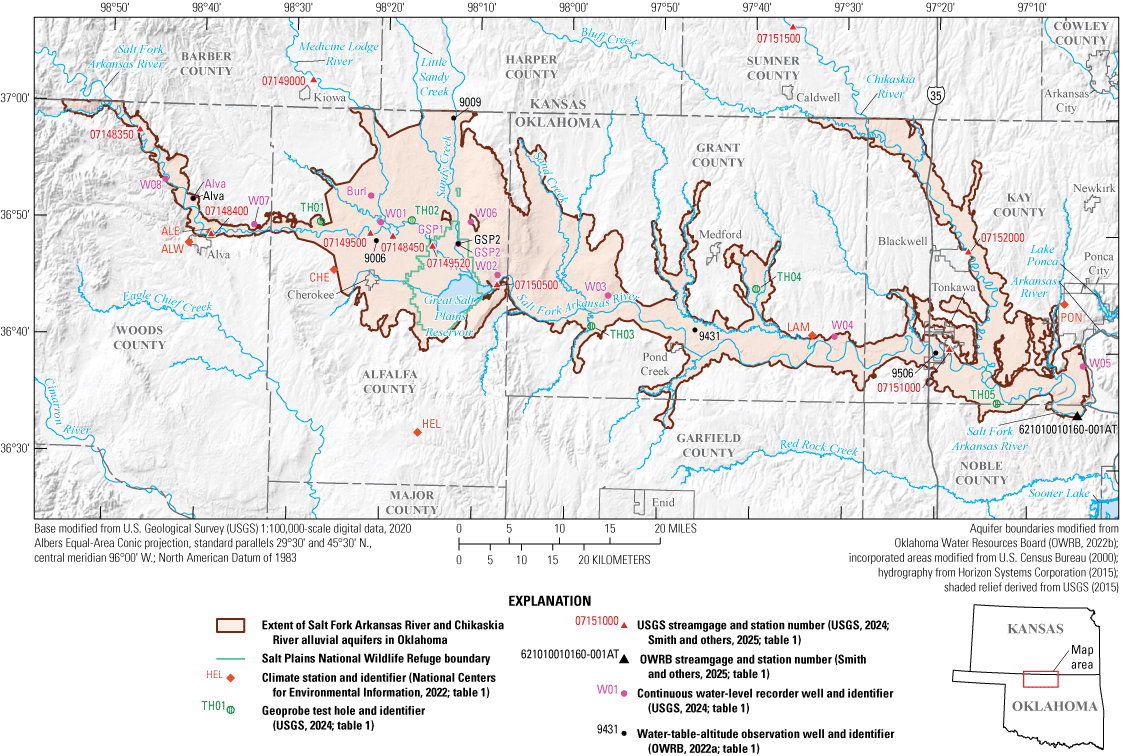
Selected data-collection stations in and near the extent of the Salt Fork Arkansas River and Chikaskia River alluvial aquifers, northern Oklahoma.
Selected data-collection stations and major geographic and surface-water features in and near the Salt Fork Arkansas River and Chikaskia River alluvial aquifers, northern Oklahoma.
River alluvial aquifers in Oklahoma were combined for this analysis (fig. 1). The Salt Fork Arkansas River alluvial aquifer is classified as a major aquifer, and the Chikaskia River alluvial aquifer is classified as a minor aquifer by the OWRB (2012a). Because the two aquifers are physically connected and presumably have the same geologic history and source material, this report generally discusses them as one entity, referred to herein as the “Salt Fork Arkansas River and Chikaskia River alluvial aquifers” unless enough data are available to describe them separately. Furthermore, when data availability allows for more detailed discussion, the Salt Fork Arkansas River alluvial aquifer is split into two reaches: one covering the part of the aquifer west of the Great Salt Plains Reservoir dam (upgradient) and the other covering the part of the aquifer east of the Great Salt Plains Reservoir dam (downgradient).
The 1973 Oklahoma Groundwater Law (Oklahoma Statute §82–1020.5 [Oklahoma State Legislature, 2021b]) requires the OWRB to conduct hydrologic investigations of the State’s aquifers (defined as groundwater basins in the statutes) to determine the maximum annual yield (MAY) for each groundwater basin. The MAY is defined as the total amount of fresh groundwater that can be annually withdrawn while ensuring a minimum 20-year life of that groundwater basin (OWRB, 2020). For alluvium and terrace groundwater basins, the 20-year life requirement is satisfied if, after 20 years of MAY withdrawals, 50 percent of the groundwater basin (hereinafter referred to as an “aquifer”) retains a saturated thickness of at least 5 feet (ft) (OWRB, 2014). Although 20 years is the minimum period required by law, the OWRB may consider management scenarios with longer periods. Once a MAY has been established, the amount of land owned or leased by a groundwater-use permit applicant determines the annual volume of water allocated to that applicant. The annual volume of groundwater allocated per acre of land is known as the equal-proportionate-share (EPS) groundwater withdrawal rate (OWRB, 2020). Computations of the EPS are complex and can benefit from a comprehensive hydrogeologic investigation and numerical groundwater-flow model of the groundwater system. The U.S. Geological Survey (USGS), in cooperation with the OWRB, conducted a hydrologic investigation of the Salt Fork Arkansas River and Chikaskia River alluvial aquifers in northern Oklahoma for the study period spanning 1980–2020 and evaluated the simulated effects of potential groundwater withdrawals on groundwater flow and availability in the Salt Fork Arkansas River alluvial aquifer to help inform the OWRB’s evaluation of the MAY for that aquifer.
A majority of the previous hydrogeologic investigations on the Salt Fork Arkansas River alluvial aquifer have been conducted in Alfalfa County near the Great Salt Plains Reservoir. Theis (1934) studied the geology of the area where the Great Salt Plains Reservoir was sited. The Great Salt Plains Reservoir was constructed by the U.S. Army Corps of Engineers (USACE) in 1941 by erecting a dam across the Salt Fork Arkansas River downstream from where it flowed through an area of salt flats. The reservoir is a saline waterbody because of the adjacent salt flats and incoming saline groundwater (USACE, 1978, 2021). Saline groundwater is defined herein as groundwater containing a total dissolved solids (TDS) concentration of 1,000 milligrams per liter (mg/L) or more (Dieter and others, 2018). The Salt Fork Arkansas River alluvial aquifer is a freshwater aquifer with high salinity, as represented by TDS concentrations of 3,770 mg/L (USGS, 2024) and chloride concentrations ranging from 205 to 29,300 mg/L (Eckenstein, 1994). Seepage from the Salt Fork Arkansas River and the upward flow of saline groundwater from the underlying bedrock are the primary sources of dissolved solids to the Salt Fork Arkansas River alluvial aquifer.
Groundwater resources of the Salt Fork Arkansas River alluvial aquifer were first studied by Schoff (1950) near Cherokee, Okla. The USACE conducted research in the area as a part of the chloride control studies and the Great Salt Plains Reservoir (USACE, 1969, 1978). Dover (1957) and Dover and others (1968) examined the water quality of the Salt Fork Arkansas River alluvial aquifer for its potential development. The groundwater resources were evaluated by Fader and Morton (1975) in Alfalfa, Grant, Kay, and Noble Counties. Hydrologic atlases were created by Bingham and Bergman (1980) and Morton (1980), presenting the geology and characterizing the water resources of the area. Eckenstein (1995) completed a hydrogeologic investigation to determine the sensitivity of groundwater in the Salt Fork Arkansas River alluvial aquifer to groundwater-withdrawal-induced infiltration. Eckenstein (1995) also evaluated the effects of surface-water discharge with high chloride concentrations from the Great Salt Plains Reservoir to the Salt Fork Arkansas River. Groundwater in wells near the Great Salt Plains Reservoir and adjoining Salt Fork Arkansas River was found to be more reactive to induced infiltration of more saline surface water in the Salt Fork Arkansas River.
Purpose and Scope
This report documents a hydrologic investigation of the Salt Fork Arkansas River and Chikaskia River alluvial aquifers in northern Oklahoma, featuring (1) an updated summary of the hydrogeologic system, with a definition of the hydrogeologic framework (including an updated spatial extent) of the aquifers, as well as the hydrologic units, hydraulic properties, and surface-water and groundwater flow characteristics of these aquifers; (2) a discussion of the development of conceptual and calibrated numerical groundwater-flow models for the aquifers representing the 1980–2020 study period; and (3) results of simulations of groundwater availability scenarios.
The construction, calibration, and use of the numerical groundwater-flow model are described to provide estimates of the response of the aquifer to transient stresses and various groundwater withdrawals and drought scenarios. The groundwater-availability scenarios use the calibrated numerical groundwater-flow model to (1) estimate the EPS groundwater withdrawal rate that could result in a minimum 20-, 40-, and 50-year life of the Salt Fork Arkansas River alluvial aquifer for which a saturated thickness of at least 5 ft remains at the end of each period; (2) quantify the potential effects of projected well withdrawals on groundwater storage in the Salt Fork Arkansas River alluvial aquifer over a 50-year period; and (3) simulate the potential effects of a hypothetical 10-year drought on groundwater storage in the Salt Fork Arkansas River alluvial aquifer. This work is based on the current understanding of the Salt Fork Arkansas River and Chikaskia River alluvial aquifer, and a comprehensive hydrologic investigation of the aquifers could improve the development of a groundwater-flow model. The calibrated numerical groundwater-flow model and groundwater-availability scenarios were archived and released in a USGS data release (Smith and Gammill, 2025).
The geographic scope of this report is the Oklahoma part of (1) the Salt Fork Arkansas River alluvial aquifer, which ends at the confluence of the Salt Fork Arkansas and Arkansas Rivers, and (2) the Chikaskia River alluvial aquifer (fig. 1). However, the Salt Fork Arkansas River alluvial aquifer was the primary focus for the collection of new data, summarization of existing data, and model simulations described in this report. For this report, the Salt Fork Arkansas River and Chikaskia River alluvial aquifers include selected alluvium, terrace, and dune deposits adjacent to major tributaries of the Salt Fork Arkansas and Chikaskia Rivers in Oklahoma (fig. 1). Selected sections in this report are modified from Ellis and others (2017; 2020), Smith and others (2021), and Rogers and others (2023). Although the study areas and aquifers of interest differ, the organization and wording of this report are largely based on Rogers and others (2023).
Description of Study Area
The Salt Fork Arkansas River and Chikaskia River alluvial aquifers are long, narrow, connected, unconfined aquifers that consist mostly of unconsolidated alluvial, terrace, and dune deposits in Alfalfa, Garfield, Grant, Kay, Noble, and Woods Counties in northern Oklahoma (fig. 1). In the eastern part of the study area, the Salt Fork Arkansas and Chikaskia Rivers are perennial except during extreme droughts, as documented by historical USGS streamgage records for each stream obtained from the USGS National Water Information System (NWIS) database (USGS, 2024; table 1). In the western part of the study area, the Salt Fork Arkansas River typically has no flow (defined herein as daily discharge less than 1 cubic foot per second) for several days per year. The Salt Fork Arkansas River generally flows west to east for about 175 miles (mi) (Horizon Systems Corporation, 2015) in Oklahoma. In the study area, the Chikaskia River generally flows north to south for about 50 mi (Horizon Systems Corporation, 2015), joining the Salt Fork Arkansas River east of Tonkawa, Okla.
Table 1.
Selected continuous record streamgages in and near the Salt Fork Arkansas River and Chikaskia River alluvial aquifers, northern Oklahoma (U.S. Geological Survey, 2024; Smith and Gammill, 2025).[U.S. Geological Survey (USGS, 2024) data can be accessed using the 8-digit station number or other identifier. NAD 83, North American Datum of 1983; M/D/Y, month/day/year; Okla., Oklahoma; Kan., Kansas; SFR2, Streamflow-Routing package; WTF, water-table-fluctuation method; OWRB, Oklahoma Water Resources Board; applicable]
| Station name | Short name for station or other identifier | Station number or identifier (fig. 1) | Latitude (decimal degrees NAD 83) | Longitude (decimal degrees NAD 83) |
County | Period of record (may contain gaps) (M/D/Y) | Contributing drainage area (square miles) |
Use in numerical groundwater-flow model | |
|---|---|---|---|---|---|---|---|---|---|
| Begin | End | ||||||||
| Salt Fork Arkansas River near Winchester, Okla. | Winchester streamgage | 07148350 | 36.9617 | −98.7823 | Woods | 10/1/1959 | 9/30/1993 | 856 | SFR2 inflow |
| Salt Fork Arkansas River near Alva, Okla. | Alva streamgage | 07148400 | 36.815 | −98.6481 | Woods | 4/1/1938 | Present | 982 | Calibration |
| Salt Fork Arkansas River near Ingersoll, Okla. | Ingersoll streamgage | 07148450 | 36.8217 | −98.3601 | Alfalfa | 9/1/1961 | 9/29/1979 | 1,140 | SFR2 inflow |
| Medicine Lodge River near Kiowa, Kan. | Kiowa streamgage | 07149000 | 37.0389 | −98.4702 | Barber (Kan.) | 2/11/1938 | Present | 903 | SFR2 inflow |
| Salt Fork Arkansas River near Cherokee, Okla. | Cherokee streamgage | 07149500 | 36.8184 | −98.3192 | Alfalfa | 10/1/1940 | 9/29/1950 | 2,439 | SFR2 inflow |
| Salt Fork Arkansas River at State Highway 11 near Cherokee, Okla. | State Highway 11 streamgage | 07149520 | 36.8056 | −98.2472 | Alfalfa | 10/1/2013 | Present | 2,365 | Calibration |
| Salt Fork Arkansas River near Jet, Okla. | Jet streamgage | 07150500 | 36.7525 | −98.129 | Alfalfa | 10/1/1937 | 9/30/1993 | 3,194 | SFR2 inflow |
| Salt Fork Arkansas River at Tonkawa, Okla. | Tonkawa streamgage | 07151000 | 36.672 | −97.3095 | Kay | 10/1/1935 | Present | 4,470 | Calibration |
| Chikaskia River near Corbin, Kan. | Corbin streamgage | 07151500 | 37.1287 | −97.6016 | Sumner (Kan.) | 8/9/1950 | Present | 794 | SFR2 inflow |
| Chikaskia River near Blackwell, Okla. | Blackwell streamgage | 07152000 | 36.8114 | −97.2773 | Kay | 4/1/1936 | Present | 1,873 | Calibration |
| Salt Fork Arkansas River near White Eagle, Okla. (OWRB) | OWRB White Eagle streamgage | 621010010160-001AT | 36.5791 | −97.0774 | Noble | 8/29/2017 | 6/30/2020 | 6,709 | Calibration |
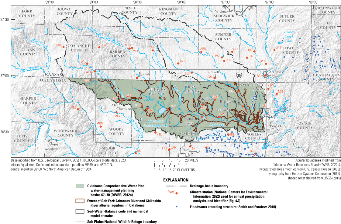
Construction of the Great Salt Plains Reservoir was authorized in 1936 for the purposes of flood control and wildlife conservation in the approximately 32,000-acre Salt Plains National Wildlife Refuge, which mostly surrounds the reservoir (USACE, 2023a; U.S. Fish and Wildlife Service, 2023). In 1941, the Great Salt Plains Reservoir was impounded on the Salt Fork Arkansas River about 70 river mi from the Kansas State line, along the eastern edge of a feature known locally, and referred to herein, as the “Great Salt plains” in northern Oklahoma (Horizon Systems Corporation, 2015). Because saline groundwater wells up to the surface from local “salt seeps,” the reservoir was not designed for use as a water supply. At a conservation-pool altitude of about 1,125 ft above the North American Vertical Datum of 1988 (NAVD 88), the reservoir is relatively shallow, with a maximum depth of about 16 ft (OWRB, 2023) and storage of about 26,000 acre-feet (acre-ft) (USACE, 2023b). The 310-ft-wide primary spillway is uncontrolled (ungated), so releases from the reservoir are continuous except during times of drought (USACE, 2023a). Unlike nearby drainage basins in Oklahoma (Ellis and others, 2020; Rogers and others, 2023), the drainage basins of the Salt Fork Arkansas and Chikaskia Rivers contain relatively few Natural Resources Conservation Service floodwater-retarding structures (fig. 2) or other large dams (associated with labeled reservoirs in fig. 2) that alter the surface-water hydrology.
Land-cover data for the Salt Fork Arkansas River and Chikaskia River alluvial aquifers study area were obtained from the CropScape database (National Agricultural Statistics Service, 2022) (fig. 3), which includes land-cover characteristics at 30-meter (m) resolution for the 2010–21 period. During this period, land-cover consisted of cropland (46.8 percent), grass or pasture (36.1 percent), developed (4.5 percent), forest or shrubland (2.7 percent), and other (9.9 percent), the last of which includes open water, wetland, and barren cover primarily in the areas near the Great Salt Plains Reservoir. Winter wheat was the major crop-cover type in the study area, accounting for 62.1 percent of cropland by area. Soybeans (12.2 percent) and alfalfa or hay (6.2 percent) were the next largest crop-cover types by area. Corn and sorghum accounted for 5.4 and 3.7 percent of cropland by area, respectively. Canola (1.3 percent), rye (1.1 percent), and fallow or idle cropland (4.6 percent) were the only other crop-cover types that accounted for more than 1 percent of cropland by area (fig. 3). Crop-cover types can change in response to economic conditions and hydrologic factors, but the percentages of total cropland cover and individual crop types did not change substantially during the 2010–21 period (National Agricultural Statistics Service, 2022).
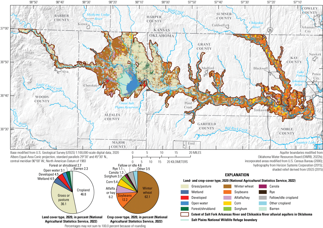
Land- and crop-cover types for land overlying the study area of the Salt Fork Arkansas River and Chikaskia River alluvial aquifers, northern Oklahoma, 2010–21.
Climate Characteristics
Historical daily data from selected climate stations in northern Oklahoma (fig. 1) were obtained from the National Centers for Environmental Information (2022) (fig. 4A, table 2). These data, which extend back to the 1890s at some locations, were summarized to tabulate and graph annual and monthly temperature and precipitation statistics for the study area (fig. 4A, table 3). A locally weighted scatterplot smoothing function line (Cleveland, 1979) with a smoothing factor of about 0.04, chosen to mimic a 5-year moving mean (5 divided by 126 annual values), was used to delineate periods of below- and above-mean annual temperature and precipitation. The mean annual precipitation during 1895–2020 was 28.9 inches (in.) (fig. 4A, table 3), and the mean annual precipitation increases by about 10.0 in. from west to east across the study area (Oklahoma Climatological Survey, 2022a, b). The mean annual precipitation for the 1980–2020 study period was 33.1 in. (fig. 4A, table 3). Within the available record, 1981–2010 was an unprecedented wet period; above-mean precipitation was recorded in 22 of these 30 years (73 percent). This wet period contributed to a higher mean precipitation during the study period compared to the mean for the period of record (fig. 4A). May is typically the wettest month, and January is typically the driest month (fig. 5A). The mean annual snowfall is about 11 in. across the western part of the study area and 8 in. across the eastern part (Oklahoma Climatological Survey, 2023). The mean annual temperature during 1895–2020 was 58.3 degrees Fahrenheit (°F) (fig. 4B, table 3), and increases by about 1 °F from east to west across the study area (Oklahoma Climatological Survey, 2022a, b; Oklahoma Mesonet, 2019).
Table 2.
Climate data-collection stations in and near the Salt Fork Arkansas River and Chikaskia River alluvial aquifers, northern Oklahoma.[U.S. Geological Survey (USGS, 2024) data can be accessed using the 8-digit station number or other identifier. NAD 83, North American Datum of 1983; M/D/Y, month/day/year; NAVD 88, North American Vertical Datum of 1988; OK, Oklahoma; US, United States; KS, Kansas; Kan., Kansas; WTF, water-table-fluctuation method; --, unknown or not applicable]
| Station name | Short name for station or other identifier | Station number or identifier (fig. 1) | Latitude (decimal degrees NAD 83) | Longitude (decimal degrees NAD 83) | County | Period of record (may contain gaps) (M/D/Y) | Land-surface altitude (feet above NAVD 88) |
Use in numerical groundwater-flow model | |
|---|---|---|---|---|---|---|---|---|---|
| Begin | End | ||||||||
| Alva 1 ENE, OK US | USC00340194 | ALE | 36.8167 | −98.65 | Woods | 5/31/1981 | 10/30/1988 | 1,293 | Recharge (WTF) |
| Alva 7 SSW Mesonet, OK US | USC00340198 | ALV | 36.7081 | −98.7094 | Woods | 5/31/2009 | Present | 1,440 | -- |
| Alva 1 W, OK US | USC00340193 | ALW | 36.8014 | −98.6878 | Woods | 3/31/1894 | Present | 1,464 | Recharge (WTF) |
| Anthony, KS US | USW00013980 | ANT | 37.155 | −98.0282 | Harper (Kan.) | 9/30/1896 | Present | 1,360 | -- |
| Argonia, KS US | USC00140308 | ARG | 37.2618 | −97.769 | Sumner (Kan.) | 3/31/1973 | Present | 1,245 | -- |
| Arkansas City, KS US | USC00140313 | ARK | 37.0631 | −97.0399 | Cowley (Kan.) | 6/30/1916 | Present | 1,118 | -- |
| Attica 6 WNW, KS US | USC00140431 | ATT | 37.2667 | −98.3167 | Harper (Kan.) | 2/28/1938 | 6/29/1993 | 1,440 | -- |
| Billings, OK US | USC00340755 | BIL | 36.5297 | −97.4472 | Noble | 2/27/1914 | Present | 1,000 | -- |
| Blackwell 4 SSE Mesonet, OK US | USC00340810 | BL4 | 36.7542 | −97.2544 | Kay | 2/27/2009 | Present | 997 | -- |
| Blackwell 1 SSW, OK US | USC00340818 | BLA | 36.7835 | −97.2901 | Kay | 4/30/1953 | Present | 1,033 | -- |
| Bluff City, KS US | USC00140926 | BLU | 37.0763 | −97.8699 | Harper (Kan.) | 3/31/1973 | Present | 1,231 | -- |
| Braman, OK US | USC00341075 | BRA | 36.9217 | −97.3356 | Kay | 5/31/2001 | 1/31/2022 | 1,050 | -- |
| Breckinridge 3 SE Mesonet, OK US | USC00341083 | BRE | 36.4119 | −97.6939 | Garfield | 2/27/2009 | Present | 1,154 | -- |
| Caldwell, KS US | USC00141233 | CAL | 37.0326 | −97.6155 | Sumner (Kan.) | 7/31/1948 | Present | 1,138 | -- |
| Cherokee 1 SSW Mesonet, OK US | USC00341726 | CH1 | 36.7481 | −98.3627 | Alfalfa | 2/27/2009 | Present | 1,187 | -- |
| Cherokee, OK US | USC00341724 | CHE | 36.7673 | −98.4244 | Alfalfa | 5/31/1915 | 2/27/2014 | 1,239 | Recharge (WTF) |
| Coldwater, KS US | USC00141704 | COL | 37.2732 | −99.3288 | Comanche (Kan.) | 2/27/1893 | Present | 2,115 | -- |
| Dalton Rome, KS US | USC00141994 | DAL | 37.2167 | −97.25 | Sumner (Kan.) | 7/31/1917 | 8/30/1922 | -- | -- |
| Enid, OK US | USC00342912 | ENI | 36.4194 | −97.8747 | Garfield | 2/27/1894 | Present | 1,245 | -- |
| Freedom 3 SSW Mesonet, OK US | USC00343363 | FR3 | 36.7256 | −99.1422 | Woodward | 2/27/2009 | Present | 1,738 | -- |
| Freedom 16 NNE Mesonet, OK US | USC00343660 | FRE | 36.9869 | −99.0108 | Woods | 2/27/2009 | Present | 1,820 | -- |
| Great Salt Plains Dam, OK US | USC00343740 | GRE | 36.7425 | −98.133 | Alfalfa | 3/11/1946 | Present | 1,200 | -- |
| Helena 1 SSE, OK US | USC00344019 | HEL | 36.538 | −98.2661 | Alfalfa | 2/27/1906 | Present | 1,350 | Recharge (WTF) |
| Jefferson 3 SE, OK US | USC00344573 | JEF | 36.6856 | −97.7486 | Grant | 2/27/1894 | Present | 1,043 | -- |
| Kiowa, KS US | USC00144341 | KIO | 37.0174 | −98.4899 | Barber (Kan.) | 2/27/1893 | Present | 1,325 | -- |
| Lahoma 1 WSW Mesonet, OK US | USC00344951 | LAH | 36.3842 | −98.1114 | Major | 2/27/2009 | Present | 1,299 | -- |
| Lamont, OK US | USC00345013 | LAM | 36.6878 | −97.5574 | Grant | 2/27/1993 | Present | 1,007 | Recharge (WTF) |
| Lahoma Research Station, OK US | USC00344950 | LRS | 36.3895 | −98.1061 | Major | 2/27/1982 | Present | 1,275 | -- |
| Medford 1 SW Mesonet, OK US | USC00345769 | ME1 | 36.7924 | −97.7458 | Grant | 2/27/2009 | Present | 1,089 | -- |
| Medford 7 ENE, OK US | USC00345768 | ME7 | 36.8384 | −97.6061 | Grant | 3/31/1981 | Present | 1,129 | -- |
| Medicine Lodge 1 E, KS US | USW00003957 | ML1 | 37.2839 | −98.5528 | Barber (Kan.) | 2/27/1998 | Present | 1,535 | -- |
| Medicine Lodge, KS US | USC00145173 | MLO | 37.2766 | −98.5799 | Barber (Kan.) | 2/27/1893 | 12/22/1998 | 1,470 | -- |
| Newkirk 8 E Mesonet, OK US | USC00346282 | NE8 | 36.8981 | −96.9104 | Kay | 2/27/2009 | Present | 1,200 | -- |
| Newkirk 5 NE, OK US | USC00346278 | NEW | 36.9423 | −97.0059 | Kay | 2/27/1898 | Present | 1,142 | -- |
| Orienta 1 SSW, OK US | USC00346751 | ORI | 36.3487 | −98.4808 | Major | 4/30/1956 | Present | 1,259 | -- |
| Oxford, KS US | USC00146169 | OXF | 37.2736 | −97.1694 | Sumner (Kan.) | 2/27/1943 | Present | 1,180 | -- |
| Perth, KS US | USC00146340 | PER | 37.1861 | −97.5086 | Sumner (Kan.) | 3/31/1973 | 8/30/2013 | 1,215 | -- |
| Ponca City Municipal Airport, OK US | USW00013969 | PON | 36.7369 | −97.1023 | Kay | 2/27/1948 | Present | 998 | Recharge (WTF) |
| Perth Near Soil Conservation Service 19s, KS US | USC00146361 | PSC | 37.2167 | −97.5333 | Sumner (Kan.) | 11/30/1940 | 12/30/1941 | 1,250 | -- |
| Red Rock 7 SSE Mesonet, OK US | USC00347507 | RED | 36.3558 | −97.1531 | Noble | 2/27/2009 | Present | 961 | -- |
| Sun City 6 S, KS US | USC00147968 | SUN | 37.2817 | −98.9251 | Barber (Kan.) | 11/30/1997 | Present | 1,963 | -- |
| Waynoka, OK US | USC00349404 | WAY | 36.5758 | −98.8797 | Woods | 3/31/1938 | Present | 1,508 | -- |
| Wellington, KS US | USC00148670 | WEL | 37.2677 | −97.4194 | Sumner (Kan.) | 3/31/1894 | Present | 1,224 | -- |
| Winfield 3 NE, KS US | USC00148964 | WI3 | 37.2885 | −96.9408 | Cowley (Kan.) | 2/28/1894 | Present | 1,233 | -- |
| Wilmore 16 SE, KS US | USC00148914 | WIL | 37.1318 | −99.0556 | Comanche (Kan.) | 8/31/1986 | 4/28/2018 | 1,667 | -- |
| Winfield Strother Field Airport, KS US | USW00013932 | WIN | 37.1649 | −97.035 | Cowley (Kan.) | 6/30/1996 | Present | 1,152 | -- |
Table 3.
Mean annual precipitation and mean annual temperature for selected periods in northern Oklahoma (1895–2020) and in the Salt Fork Arkansas River alluvial aquifer both upgradient and downgradient from the Great Salt Plains Reservoir (1980–2020) (National Centers for Environmental Information, 2022).[Okla., Oklahoma; --, data not summarized]
| Region or location | Period | Number of years | Mean annual precipitation (inches) | Mean annual temperature (degrees Fahrenheit) |
|---|---|---|---|---|
| Northern Oklahoma (data summarized from climate stations in table 2 and fig. 2) | 1895–2020 | 126 | 28.9 | 58.3 |
| Same as above | 1895–1936 | 42 | 28.3 | 58.0 |
| Same as above | 1937–1978 | 42 | 28.2 | 58.1 |
| Same as above | 1979–2020 | 42 | 33.1 | 58.7 |
| Same as above | 1980–2020 | 41 | 33.1 | 58.7 |
| Salt Fork Arkansas River alluvial aquifer upgradient from Great Salt Plains Reservoir (Helena, Okla., station USC00344019; HEL, table 2, fig. 2)1 | 1980–2020 | 41 | 31.4 | -- |
| Salt Fork Arkansas River alluvial aquifer downgradient from Great Salt Plains Reservoir (Billings, Okla., station USC00340755; BIL, table 2, fig. 2) | 21980–2020 | 41 | 35.1 | -- |
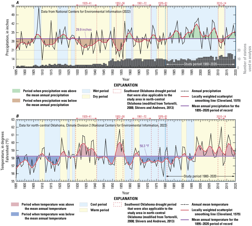
A, Long-term precipitation and wet and dry periods, and B, long-term temperature and cool and warm periods, northern Oklahoma, 1895–2020 (National Centers for Environmental Information, 2022).
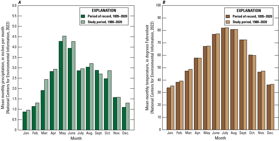
A, Mean monthly precipitation, and B, mean monthly temperature in northern Oklahoma for 1895–2020 and 1980–2020 (National Centers for Environmental Information, 2022).
Multiyear to decadal droughts are common in Oklahoma (Moreland, 1993). The 1929–41 (“Dust Bowl,” Egan, 2006) and 1952–56 drought periods were among the most severe in Oklahoma in the 20th century; two shorter, less severe drought periods also occurred later in the 20th century, during 1961–72 and 1976–81 (fig. 4A) (Tortorelli, 2008; Shivers and Andrews, 2013). The most severe droughts on record developed from extended periods of below-mean precipitation paired with above-mean temperature.
Streamflow Characteristics and Trends
Daily streamflow data, with varying and sometimes interrupted periods of record, were recorded at selected USGS streamgages in the study area (fig. 1) and summarized for the 1980–2020 study period (tables 4, 5). Daily streamflow data were also collected at one OWRB streamgage in the study area, OWRB streamgage 621010010160-001AT near White Eagle, Okla. (hereinafter referred to as the “OWRB White Eagle streamgage”). OWRB White Eagle streamgage data were provided as furnished record (Derrick Wagner, Technical Studies Manager, Oklahoma Water Resources Board, 2023) and are published in the companion USGS data release (Smith and Gammill, 2025). Streamflow measured at streamgages is the sum of runoff and base flow originating upstream; base flow is the component of streamflow supplied by the discharge of groundwater to streams (Barlow and Leake, 2012). For this report, streamflow-hydrograph data obtained from the NWIS database (USGS, 2024) were separated into runoff and base-flow components by using the standard Base-Flow Index code (Wahl and Wahl, 1995) in the USGS Groundwater Toolbox (Barlow and others, 2015). The Base-Flow Index code uses the minimum streamflow in a moving n-day window as a basis for hydrograph separation; for consistency, a 5-day window was used for all streamgages listed in this report. The 5-day window was selected by testing multiple n-day windows for the study period at USGS streamgage 07151000 Salt Fork Arkansas River at Tonkawa, Okla. (hereinafter referred to as the “Tonkawa streamgage”) and plotting the resulting mean base-flow percentage against n; a slope change was evident at 5 days. Base flow, as computed by using this method, generally accounts for about 15–60 percent of annual streamflow for the periods of record at the Tonkawa streamgage (fig. 6C) and at USGS streamgage 07152000 Chikaskia River near Blackwell, Okla. (hereinafter referred to as the “Blackwell streamgage”) (fig. 6E). This percentage, known as the base-flow index (BFI) (Wahl and Wahl, 1995; Barlow and others, 2015), generally increased annually over the period of record through 2021 at streamgages on the Salt Fork Arkansas, Medicine Lodge, and Chikaskia Rivers (fig. 6A–E).
Table 4.
Annual streamflow and base-flow values for selected U.S. Geological Survey streamgages upgradient from Great Salt Plains Reservoir in and near the surficial extents of the sediments that contain the Salt Fork Arkansas River and Chikaskia River alluvial aquifers, northern Oklahoma, for the parts of their differing periods of record that occurred during the period 1936–2021 and during the study period 1980–2020.[Great Salt Plains Reservoir releases from U.S. Army Corps of Engineers (2023b). Other streamflow data from the U.S. Geological Survey (USGS) National Water Information System (USGS, 2024). All base-flow values computed by using the Base-Flow Index code (Wahl and Wahl, 1995) in the USGS Groundwater Toolbox (Barlow and others, 2015) are reported in units of cubic feet per second. The base-flow index value for a USGS streamgage can be calculated for any year or period by dividing the mean base flow value by the mean streamflow value. Streamgage locations shown on figure 1. The period of record is 1980–2020. Okla., Oklahoma; Kan., Kansas; POR, period of record; --, data not available or not applicable]
Table 5.
Annual streamflow and base-flow values for selected U.S. Geological Survey streamgages downgradient from Great Salt Plains Reservoir in and near the surficial extents of the sediments that contain the Salt Fork Arkansas River and Chikaskia River alluvial aquifers, northern Oklahoma, for the parts of their differing periods of record that occurred during the period 1936–2021 and during the study period 1980–2020.[Great Salt Plains Reservoir releases from U.S. Army Corps of Engineers (2023b). Other streamflow data from the U.S. Geological Survey (USGS) National Water Information System (USGS, 2024). All base-flow values computed by using the Base-Flow Index code (Wahl and Wahl, 1995) in the USGS Groundwater Toolbox (Barlow and others, 2015) are reported in units of cubic feet per second. The base-flow index value for a USGS streamgage can be calculated for any year or period by dividing the mean base flow value by the mean streamflow value. Streamgage locations shown on figure 1. The period of record is 1980–2020. Okla., Oklahoma; Kan., Kansas; POR, period of record; --, data not available or not applicable]
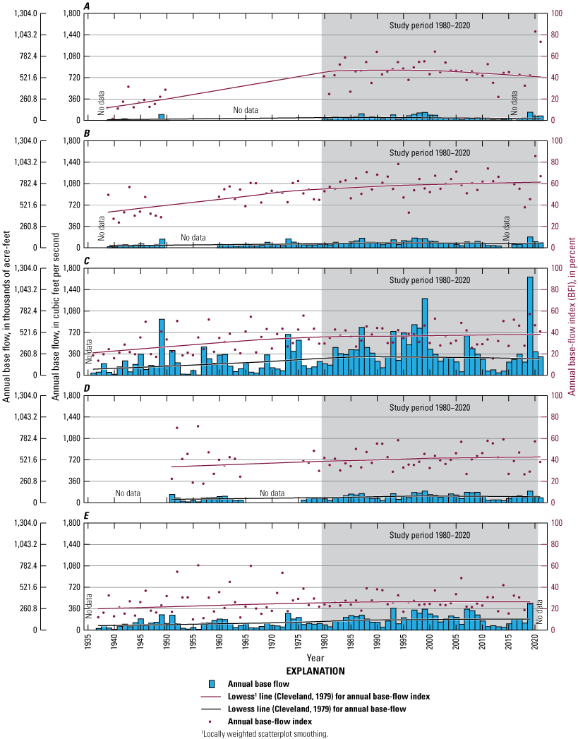
Annual base-flow and annual base-flow index values for U.S. Geological Survey streamgages A, 07148400 Salt Fork Arkansas River near Alva, Oklahoma; B, 07149000 Medicine Lodge River near Kiowa, Kansas; C, 07151000 Salt Fork Arkansas River at Tonkawa, Okla.; D, 07151500 Chikaskia River near Corbin, Kan.; and E, 07152000 Chikaskia River near Blackwell, Okla., in and near the Salt Fork Arkansas River alluvial aquifer study area, northern Oklahoma, for their varying periods of record that occurred during the period from 1936 to 2021 (U.S. Geological Survey, 2024).
Annual BFI, base-flow, and streamflow trends described in this report were analyzed by using the Kendall tau test (Kendall, 1938) (kendalltau, SciPy version 1.7.1 [Virtanen and others, 2020]) with the Theil-Sen slope estimator (Sen, 1968) (theilslopes, SciPy version 1.7.1 [Virtanen and others, 2020]) and specifying an alpha value of 0.05 as the significance level. Statistically significant upward or downward trends are indicated when the probability value (p-value) is less than the alpha value (Helsel and others, 2020). For the full period of record, the upward trends in the BFI were found to be statistically significant (p-value = 0.0002) at USGS streamgage 07148400 Salt Fork Arkansas River near Alva, Okla. (hereinafter referred to as the “Alva streamgage”), statistically significant (p-value < 0.0001) at USGS streamgage 07149000 Medicine Lodge River near Kiowa, Kan. (hereinafter referred to as the “Kiowa streamgage”), and statistically significant (p-value = 0.0001) at the Tonkawa streamgage. The upward trends in the BFI were found to be not statistically significant (p-values = 0.2135 and 0.0856, respectively) at USGS streamgages on the Chikaskia River, which included USGS streamgage 07151500 Chikaskia River near Corbin, Kan. (hereinafter referred to as the “Corbin streamgage”) and the Blackwell streamgage. Statistically significant upward trends in base flow were detected in the streamflow records at all streamgages, but upward trends in the BFI were not always associated with upward trends in base flow. For the full period of record, the upward trends in base flow were statistically significant at all stations except the Alva streamgage, where the p-value was 0.0592. However, a 29-year data gap in the Alva streamgage record (fig. 6A) complicates the evaluation of trends at this site.
For the full period of record, upward patterns in streamflow were evident in the streamflow records for all streamgages except for the Alva streamgage; however, statistically significant upward trends in streamflow were detected only at the Tonkawa streamgage (p-value = 0.0186) and the Blackwell streamgage (p-value = 0.0069). Greater amounts of precipitation during the 1980–2020 study period (relative to the preceding period of record) were likely the primary cause of upward patterns and statistically significant trends in streamflow.
No statistically significant trends were found in BFI, base flow, or streamflow for the 1980–2020 study period. This lack of significant trends in BFI, base flow, and streamflow over the study period (paired with the presence of significant trends in BFI, base flow, and streamflow over the full period of record) indicates that the hydrologic changes responsible for the expression of trends likely occurred prior to the study period and did not continue into the study period.
Groundwater Use
The OWRB permits and regulates groundwater withdrawals of 5 acre-feet per year (acre-ft/yr) or more used for domestic and agricultural purposes and groundwater withdrawals used for irrigating more than 3 acres of land for growing gardens, orchards, or lawns (Oklahoma Statute §82–1020.1 [Oklahoma State Legislature, 2021a, OWRB, 2014]; Oklahoma Statute §82–1020.3 [Oklahoma State Legislature, 2021c]). Groundwater-use data since 1980 are self-reported annually to the OWRB by permitted users; OWRB staff compiled and reviewed groundwater-use data described in this report to ensure the quality and completeness of the data (Smith and Gammill, 2025). For the purposes of this study, all groundwater use was assumed to be consumptive use (That is, none of the groundwater withdrawn returns to the aquifer or streams.)
Most groundwater-use permits for the Salt Fork Arkansas River alluvial aquifer were allocated for irrigation or public supply, but some were allocated for other uses, including commercial, industrial, mining (including oil and gas), recreation, fish, and wildlife (fig. 7) (Smith and others, 2021; OWRB, 2022d). The Salt Fork Arkansas River alluvial aquifer can yield about 100–200 gallons per minute (OWRB, 2012a). In 2020, about 120 long-term temporary (regular) groundwater-use permits and about 80 prior-right groundwater-use permits were active for the Salt Fork Arkansas River alluvial aquifer, and 3 long-term temporary (regular) groundwater-use permits and 3 prior-right groundwater-use permits were active for the Chikaskia River alluvial aquifer (OWRB, 2022d). Each permit is tied to a land area and well location (or locations) designated for a single groundwater-use type (fig. 7).
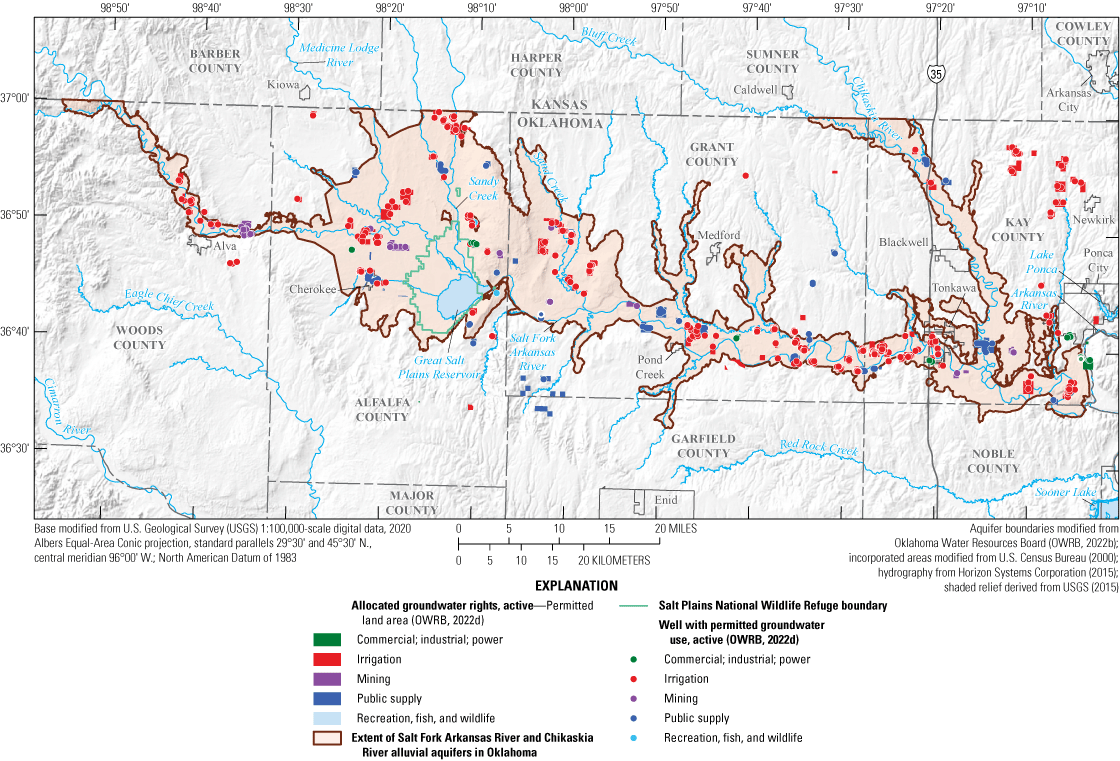
Land areas and wells permitted for groundwater use from the Salt Fork Arkansas River and Chikaskia River alluvial aquifers, northern Oklahoma, 2020.
Since 1980, the OWRB has required irrigation permit holders to report annual groundwater use in terms of the number of applications and number of inches of water applied per application (OWRB, 2024). Prior to 1980, however, the number of inches of water applied during irrigation was not required to be reported. As a result, the OWRB adopted rules to estimate the number of inches of water applied for pre-1980 data based on the number of water applications (OWRB, 2014). This change in estimation methods results in what appears to be a step-change decrease in irrigation groundwater use after 1980 (fig. 8).
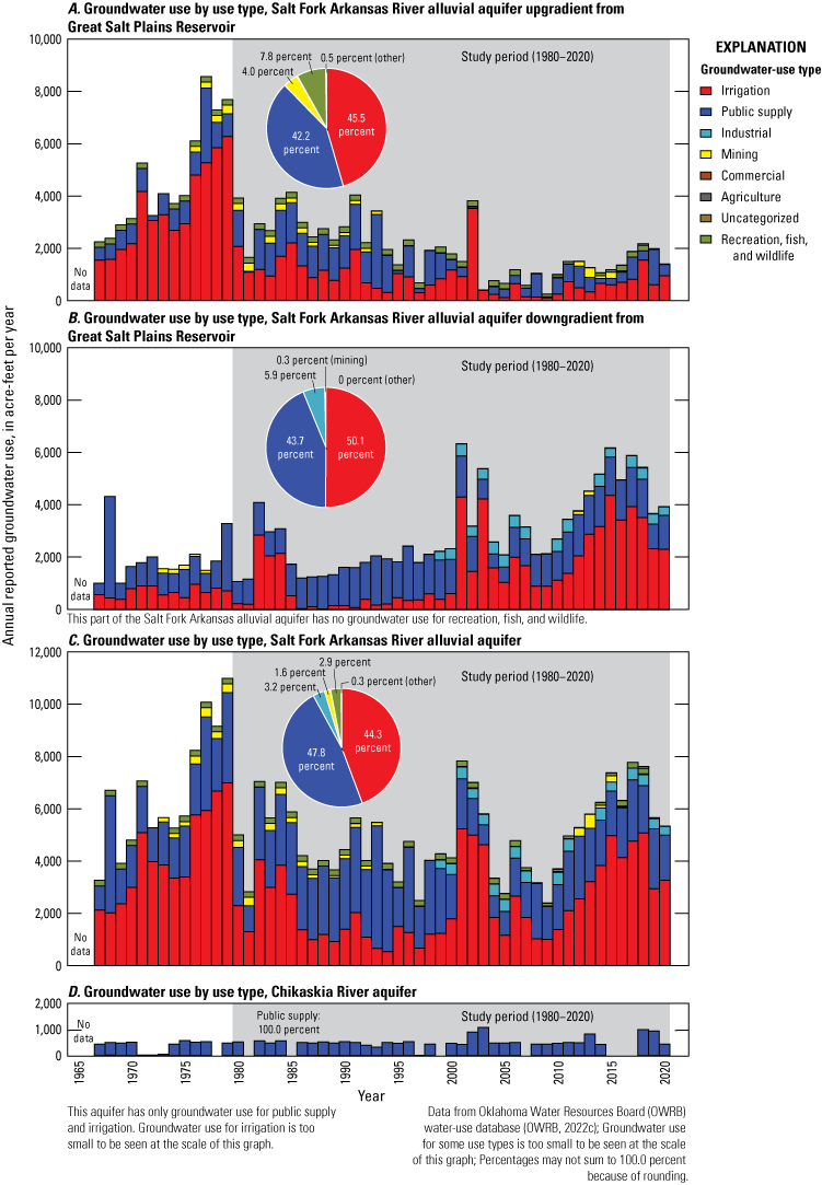
Annual reported groundwater use by use type from the Salt Fork Arkansas River and Chikaskia River alluvial aquifers, northern Oklahoma, 1967–2020. A, Upgradient from the Great Salt Plains Reservoir, B, downgradient from the Great Salt Plains Reservoir, C, Salt Fork Arkansas River alluvial aquifer, and D, Chikaskia River aquifer.
Groundwater use for domestic supply (self-supplied directly to a residence by a private well) was assumed to be a negligible part of the total groundwater use. The study area is mostly rural, with a small, widely dispersed population that relies on private wells; most of the population is concentrated in cities, where the water is supplied by municipal or rural water districts rather than by private wells.
OWRB reported groundwater use data were compiled for the 1967–2020 period of record (fig. 8; tables 6, 7) and summarized for the 1980–2020 study period (OWRB, 2024; Smith and Gammill, 2025). During the 1980–2020 study period, annual reported groundwater use in the Salt Fork Arkansas River alluvial aquifer upgradient from the Great Salt Plains Reservoir was primarily for irrigation (45.5 percent) and public supply (42.2 percent), with secondary groundwater use for recreation, fish, and wildlife (7.8 percent) and mining (4.0 percent) (fig. 8A). Annual reported groundwater use in the Salt Fork Arkansas River alluvial aquifer downgradient from the Great Salt Plains Reservoir was primarily for irrigation (50.1 percent) and public supply (43.7 percent) with secondary groundwater use for industrial (5.9 percent) purposes (fig. 8B). For the entire Salt Fork Arkansas River alluvial aquifer, annual reported groundwater use for the study period was about 5,550 acre-ft/yr (tables 6, 7), of which about 44.3 percent was for irrigation, 47.8 percent was for public supply, 3.2 percent was for industrial, 2.9 percent was for recreation, fish, and wildlife, and 1.6 percent was for mining use (fig. 8C). Annual reported groundwater use in the Salt Fork Arkansas River alluvial aquifer decreased upgradient from, and increased downgradient from, the Great Salt Plains Reservoir over the 1980–2020 study period (fig. 8A–B). The decreased groundwater use upgradient from the Great Salt Plains Reservoir over the 1980–2020 study period was caused by a combination of decreased irrigation and public-supply use, whereas the increased groundwater use downgradient was mostly caused by increased irrigation use. Annual reported groundwater use in the Chikaskia River alluvial aquifer was almost exclusively for public supply by the City of Tonkawa (fig. 8D), which reported annual groundwater use from 0 to approximately 1,100 acre-ft/yr during the 1980–2020 study period (tables 6, 7). Some of the reported groundwater-use values of 0 acre-ft/yr may be due to a lack of reporting rather than an actual estimate of how much groundwater was used. Groundwater use from the Salt Fork Arkansas River and Chikaskia River alluvial aquifers (in the Upper Arkansas planning region [OWRB, 2012a]) is projected to increase by 42 percent from 2010 to 2060; the greatest growth in projected groundwater use is expected to be for municipal (public supply), industrial, oil and gas (mining), and crop irrigation uses (OWRB, 2012a).
Table 6.
Annual reported groundwater use from the Salt Fork Arkansas River aquifer, northern Oklahoma, 1967–2020.[Permit-level reported groundwater-use data from the Oklahoma Water Resources Board (OWRB) were aggregated by groundwater-use type in this table (Rogers and others, 2023) owing to restrictions of proprietary interest and permit-holder anonymity; table excludes groundwater use of less than 5 acre-feet per year for domestic and agricultural purposes and groundwater use for irrigation of fewer than 3 acres of land for growing of gardens, orchards, or lawns (Oklahoma Statute §82–1020.3; Oklahoma State Legislature, 2021c). All values are in units of acre-feet per year. Totals may not equal sum of components because of independent rounding. The study period data are from 1980 to 2020]
Table 7.
Annual reported groundwater use from the Chikaskia River aquifer, northern Oklahoma, 1967–2020.[Permit-level reported groundwater-use data from the Oklahoma Water Resources Board (OWRB) were aggregated by groundwater-use type in this table (Rogers and others, 2023) owing to restrictions of proprietary interest and permit-holder anonymity; table excludes groundwater use of less than 5 acre-feet per year for domestic and agricultural purposes and groundwater use for irrigation of fewer than 3 acres of land for growing of gardens, orchards, or lawns (Oklahoma Statute §82–1020.3; Oklahoma State Legislature, 2021c). All values are in units of acre-feet per year. Totals may not equal sum of components because of independent rounding. The study period data are from 1980 to 2020. --, not applicable]
Hydrogeology of the Salt Fork Arkansas River and Chikaskia River Aquifers and Surrounding Units
The Quaternary alluvium, terrace, dune, and gypsum deposits of the Salt Fork Arkansas River and Chikaskia River alluvial aquifers overlie Permian bedrock units (fig. 9). The Permian bedrock units are generally composed of shale, siltstone, and fine-grained sandstone that serve as confining units in relation to the alluvium and terrace deposits of the Salt Fork Arkansas River and Chikaskia River alluvial aquifers (fig. 10). In the discussion herein, the geologic units of the study area are presented in reverse chronological order, which is the order in which the units are crossed by the Salt Fork Arkansas River in upstream to downstream order.
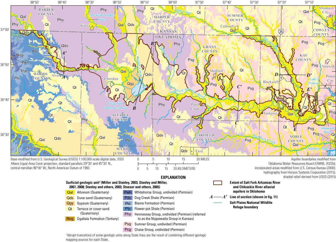
Surficial geologic units in and near the Salt Fork Arkansas River and Chikaskia River alluvial aquifers, northern Oklahoma.
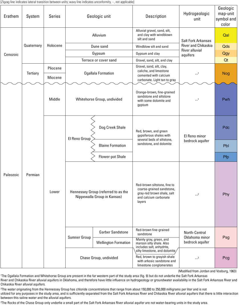
Surficial geologic and hydrogeologic units in and near the Salt Fork Arkansas River and Chikaskia River alluvial aquifers, northern Oklahoma. Because the Ogallala Formation and Whitehorse Group do not underlie the Salt Fork Arkansas River and Chikaskia River alluvial aquifers in Oklahoma, the hydrogeologic units contained in them do not interact with the Salt Fork Arkansas River and Chikaskia River alluvial aquifers.
Alluvium and Terrace Deposits
The Quaternary deposits that contain the Salt Fork Arkansas River and Chikaskia River alluvial aquifers consist primarily of alluvium and terrace deposits, gypsum, and windblown dune sands (now covered by vegetation). These Quaternary deposits are mostly composed of gravel, sand, silt, and clay and overlie the Permian geologic units (figs. 10–11). In western Grant County and northeastern Alfalfa County, thick and broad deposits of dune sands (fig. 11B) extend from southeast of the Salt Plains National Wildlife Refuge northward across the Kansas border (Eckenstein, 1995). Quaternary deposits are thickest around the Salt Plains National Wildlife Refuge and thin to the east along the Salt Fork Arkansas River, ranging from 1 to 20 mi wide throughout.
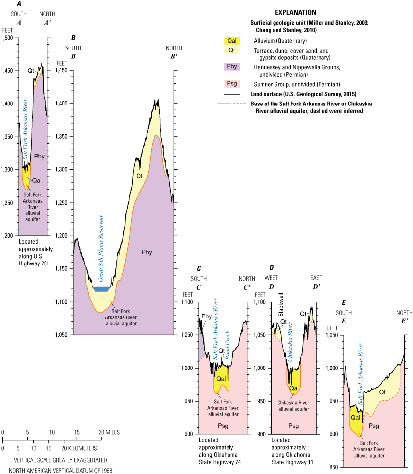
Hydrogeologic cross sections A–A′ to E–E′ of the Salt Fork Arkansas River and Chikaskia River alluvial aquifers, northern Oklahoma, at various locations (fig. 9) in the study area.
The salt flats are a featureless, unvegetated, gypsite-salt-encrusted surface covering about 25 square miles in central Alfalfa County inside the Salt Plains National Wildlife Refuge (figs. 1, 9). This area consists of loose Quaternary deposits of fluvial and lacustrine origin that are saturated with a natural brine that seeps up from the underlying Permian bedrock (USACE, 1978). This brine contains elevated concentrations of sodium chloride and calcium sulfate dissolved from evaporite deposits in the underlying Permian bedrock (Johnson, 1972). When this brine evaporates, it precipitates salt crusts on the surface and selenite gypsum crystals just below the surface (USACE, 1978).
During the Permian, an inland sea deposited layers of interbedded halite and gypsum salts (Jordan and Vosburg, 1963). There is salt dissolution across the Permian Hennessey Group, with some brine migrating upward upon reaching the artesian zones of sandstone and siltstones (Davis, 1968). The water originating from the Hennessey Group has chloride concentrations that range from about 150,000 to 250,000 milligrams per liter (mg/L) (Johnson, 1972). For a frame of reference, the total salinity of seawater is only about 35,000 mg/L. The Great Salt Plains Reservoir has a lower salinity because of the dilution effect of surface water, having about 15,000 mg/L of dissolved salts in water, which is about half that of seawater. The salinity of the reservoir varies, but the amount of salt that flows out of the reservoir through the Salt Fork Arkansas River averages about 3,000 tons per day (Johnson, 1972). Attempting to mitigate the adverse effects of salinity migration downstream, the USACE has tried to control the large concentrations of chloride by creating brine pools and constructing the Great Salt Plains Reservoir (USACE, 1978).
Bedrock Units
The Ogallala Formation of Tertiary age and Whitehorse Group of Permian age are present in the far western part of the study area (fig. 9) but do not underlie the Salt Fork Arkansas River and Chikaskia River alluvial aquifers in Oklahoma. These units, therefore, have little effect on groundwater flow and quality in the Salt Fork Arkansas River and Chikaskia River alluvial aquifers.
The bedrock units that underlie the Salt Fork Arkansas River and Chikaskia River alluvial aquifers are of Permian age and primarily composed of shale, siltstone, and fine-grained sandstone (Bingham and Bergman, 1980; Morton, 1980). The Permian El Reno Group, which includes the Dog Creek Shale, Blaine Formation, and Flower-pot Shale, is composed of red, brown, and green gypsiferous shales as well as several beds of siltstone, sandstone, and dolomite (fig. 10). Because the siltstones and sandstones are locally transmissive enough to support low-yielding groundwater production wells, the El Reno Group is considered a minor aquifer in the study area (OWRB, 2012a). The Hennessey Group consists of fine to coarse grained sandstone, red-brownish siltstone, gray to red brown shale, and salt and calcium carbonate layers (Jordan and Vosburg, 1963). The Permian Garber Sandstone of the Sumner Group is composed of red-brown fine-grained sandstone that grades northward into shale and siltstone (Bingham and Bergman, 1980; Morton, 1980). Geologic mapping by Stanley and Miller (2007) indicated that this unit thins northward and pinches out before reaching the Salt Fork Arkansas River. The Permian Wellington Formation of the Sumner Group consists mainly of gray, green, and maroon silty shale, and also includes salt, anhydrite, silty limestone, and dolomite. The Garber Sandstone and the Wellington Formation collectively contain the North-central Oklahoma minor bedrock aquifer (Bingham and Bergman, 1980; Morton, 1980). The Permian Chase Group is the oldest bedrock unit in the study area and consists of red and brown to grayish shale with arkosic sandstone and limestone conglomerates (Bingham and Bergman, 1980). Rocks of the Chase Group only underlie a small part of the Salt Fork Arkansas River alluvial aquifer.
The bedrock units that underlie the Salt Fork Arkansas River and Chikaskia River alluvial aquifers dip south and southwest in the western half of the study area (Bingham and Bergman, 1980; Morton, 1980). In the eastern part of the study area, the bedrock units dip to the west and southwest, and the regional dip is about 40 feet per mile (Bingham and Bergman, 1980; Morton, 1980). Intermittent bedrock layers of evaporites composed of halite (sodium chloride) and gypsum/anhydrite (calcium sulfate) occur in the bedrock layers of the Hennessey Group in Woods and Alfalfa Counties; when exposed to water, these evaporites dissolve to form brines that discharge at and near the land surface in Alfalfa County (USACE, 1969; Morton, 1980). The subsequent evaporation of brines that discharge at the land surface forms halite and selenite gypsum crystals in an area of about 25 square miles within the Salt Plains National Wildlife Refuge (fig. 1) (USACE, 1978; Morton, 1980). Evaporite layers are absent in bedrock layers east of Alfalfa County (Jordan and Vosburg, 1963, plate 1; USACE, 1969). In the study area, erosional processes have exposed parts of the bedrock units at land surface, forming gently rolling hills broken up by escarpments capped by resistant sandstones and limestones and valleys of shale (USACE,1969). Most of the deposition of the study area took place in restricted, saline marine environments, which are defined as having two or more entrance channels or inlets and sufficient water circulation because of tidal currents and wind effects. These types of depositional environments are responsible for the highly soluble constituents, such as halite, gypsum, and dolomite, present in the study area (USACE, 1978).
Groundwater and Surface-Water Quality
The Salt Fork Arkansas River alluvial aquifer is a freshwater aquifer with areas of saline groundwater that locally may limit its use for public supply and other selected uses. Seepage from the Salt Fork Arkansas River and the localized upward flow of saline groundwater from the underlying bedrock are the primary sources of TDS that contribute to the salinity of the aquifer. The highest TDS concentrations in the Salt Fork Arkansas River alluvial aquifer (3,770 mg/L) were measured near the Great Salt Plains Reservoir, where groundwater brines from the underlying bedrock unit, the Hennessey Group, discharge at the surface. The least saline groundwater (80 mg/L TDS) was contained in windblown dune sands northeast of the Great Salt Plains Reservoir.
Complete major-ion groundwater-quality data are useful for evaluating the salinity of water but were not available for the Chikaskia River alluvial aquifer (all analyses were lacking bicarbonate concentrations). Partial major-ion groundwater-quality data (Bingham and Bergman, 1980) indicate the groundwater in the Chikaskia River alluvial aquifer may be more saline in some locations than groundwater in the Salt Fork Arkansas River alluvial aquifer.
The salinity of surface water in the Salt Fork Arkansas River in the study area varies depending on location and flow conditions. In general, the surface water is slightly to moderately saline, with salinity concentrations of 1,000–3,000 mg/L and 3,000–10,000 mg/L, respectively (Winslow and Kister, 1956). Mean TDS concentrations of the Salt Fork Arkansas River range from about 1,500 mg/L at the Alva streamgage in Woods County to about 6,000 mg/L at USGS streamgage 07150500 Salt Fork Arkansas River near Jet, Okla. (hereinafter referred to as the “Jet streamgage”) in Alfalfa County (fig. 1) (USGS, 2024). Water released from the Great Salt Plains Reservoir is the primary source of salinity to the Salt Fork Arkansas River and the Salt Fork Arkansas River alluvial aquifer in Grant and Kay Counties (Eckenstein, 1994). Salinity of the Salt Fork Arkansas River decreases with distance downstream from the Great Salt Plains Reservoir because of dilution by freshwater tributary inflows in Grant and Kay Counties (Eckenstein, 1994).
A combination of recently collected and historical groundwater quality data and historical surface-water quality data were used in this analysis. Groundwater-quality data for the Salt Fork Arkansas River alluvial aquifer were collected by the OWRB as part of the Groundwater Monitoring and Assessment Program (GMAP) (OWRB, 2018). Groundwater samples were collected from 30 wells during July–August 2014 (fig. 12) and analyzed for physicochemical properties (dissolved oxygen, pH, specific conductance, and temperature), major ions, nitrate plus nitrite (as nitrogen), and selected trace metals. To describe groundwater quality in parts of the aquifer where GMAP wells were absent, historical data collected from 11 wells were used in this analysis. The historical groundwater quality data were retrieved from the USGS National Water Information System (NWIS) database (USGS, 2024) and consisted of major ions and nitrate (as nitrogen) concentrations measured in groundwater samples collected during 1948–72. Historical water-quality data measured in surface-water quality samples collected from seven selected sites on the Salt Fork Arkansas River during 1948–72 were used to help identity mixtures of fresh water and saline water in the aquifer; the surface-water quality data were also retrieved from the NWIS database (fig. 12).
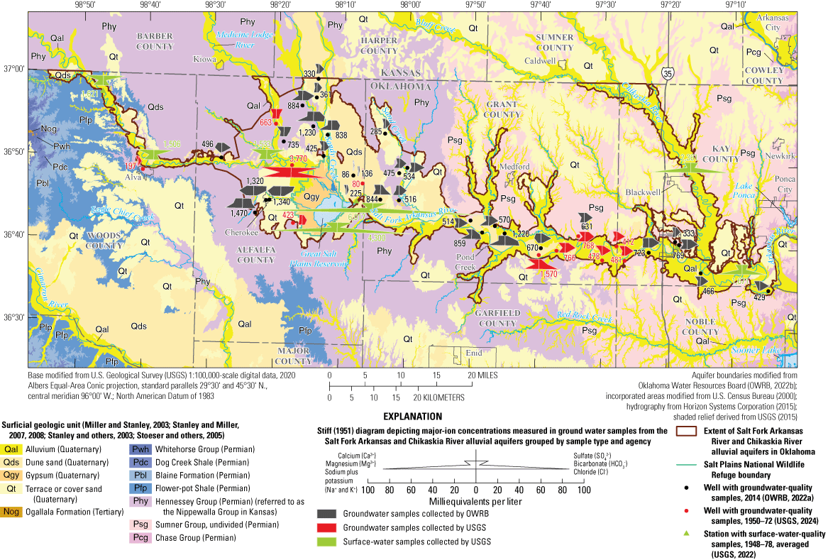
Surficial geologic units and Stiff (1951) diagrams representing groundwater- and surface-water-quality samples of water produced from the Salt Fork Arkansas River alluvial aquifer, northern Oklahoma, 1948–78 and 2014.
A statistical summary of 30 OWRB samples from the GMAP program (OWRB, 2018) was analyzed for pH, TDS, hardness constituents, sulfate, and chloride concentrations. The GMAP report indicates that groundwater from the Salt Fork Arkansas River alluvial aquifer tends to have a neutral pH, with a median pH value of 7.1 standard units. Of 30 samples, 1 was below the secondary maximum contaminant level (SMCL) for pH (6.5 SU) in finished drinking water (U.S. Environmental Protection Agency [EPA], 2017, 2020a). TDS concentrations ranged from 86.3 to 1,470 mg/L, with a median of 552 mg/L. Of 30 samples, 18 exceeded the SMCL of 500 mg/L for TDS, 5 of which would qualify as slightly saline (1,000–3,000 mg/L, as defined in Winslow and Kister [1956]) with TDS concentrations ranging from 1,220 to 1,470 mg/L (OWRB, 2018). Hardness as calcium carbonate ranged from 41.0 to 872 mg/L, with a median concentration of 348 mg/L. Of 30 samples, 27 had TDS concentrations exceeding 225 mg/L and are classified as hard, with hardness as calcium carbonate values exceeding 180 mg/L (Hem, 1985; OWRB, 2018). Concentrations of sulfate ranged from less than 10.0 to 508 mg/L with a median of 66.1 mg/L. Of 30 samples, 4 exceeded the SMCL of 250 mg/L for sulfate in finished drinking water (EPA, 2020a). Concentrations of chloride ranged from less than 10 to 398 mg/L, with a median of 55.3 mg/L. Of 30 samples, 5 exceeded the SMCL of 250 mg/L for chloride (EPA, 2020a).
Three Federally regulated water-quality constituents (nitrate plus nitrite measured as nitrogen, arsenic, and uranium) were measured in 30 samples collected by OWRB and USGS at concentrations exceeding their respective EPA maximum contaminant levels (MCL) for finished drinking water (EPA, 2017, 2020b). The water-quality data for these 30 samples are stored in the USGS NWIS database (USGS, 2024). Concentrations of nitrate plus nitrite ranged from less than 0.05 to 20.0 mg/L, with a median concentration of 4.14 mg/L; in the 30 samples collected by OWRB (2018), 5 of which exceeded the MCL of 10 mg/L. Concentrations of nitrate (as nitrogen) in the 12 USGS groundwater samples ranged from 0.05 to 36 mg/L, and 4 of the 12 samples exceeded the MCL (OWRB, 2018).
Concentrations of dissolved arsenic and uranium measured in samples collected by OWRB were evaluated and compared to their respective MCLs. Concentrations of dissolved arsenic exceeded the MCL of 10.0 micrograms per liter (µg/L) in 1 of the 30 OWRB samples; in 4 samples, the dissolved arsenic concentrations were less than the laboratory reporting level of 1.0 µg/L (OWRB, 2018). The median dissolved arsenic concentration was 2.0 µg/L. Concentrations of dissolved uranium exceeded the MCL of 30.0 µg/L in one of the 30 OWRB samples at 30.9 µg/L; the dissolved uranium concentration was less than the laboratory reporting level of 1 µg/L in 2 of the samples (OWRB, 2018). The median concentration of dissolved uranium in 30 samples was 4.7 µg/L. Uranium and arsenic were not analyzed in conjunction with the 12 USGS groundwater samples.
Cation-anion balances were used to determine water types for the groundwater samples collected at the 28 OWRB and 11 USGS groundwater-quality sites, and at 7 USGS surface-water-quality sites on the Salt Fork Arkansas River. These analyses were determined by first converting major-ion concentrations to milliequivalents per liter. When the milliequivalent concentrations of cations and anions balance within acceptable limits, they can be used to determine the water type of a given sample (Hem, 1985). For this study, cation-anion balances within 7 percent were considered acceptable for determining water types (Hem, 1985). The cation-anion balances of the major-ion concentrations were within 7.0 percent in 26 of the 28 OWRB groundwater samples, and of 11 USGS water-quality samples, 3 were above 7.0 percent (one of which was a groundwater sample and the other two surface water not sampled in the aquifer). The USGS surface and groundwater-quality sites were represented as the median major-ion concentrations from available samples.
Stiff diagrams and Piper diagrams were used to better understand variations in water types and the mixing of saline and fresh water. Groundwater- and surface-water-quality data were plotted on Stiff (1951) diagrams for visual comparisons (fig. 12). Stiff diagrams (Stiff, 1951) are visual representations of major-ion concentrations showing the dominant water type. These diagrams were made by using the Python WQChartPy package (Yang and others, 2022) to compare and interpret the water-quality data. The dominant water type in the Salt Fork Arkansas River varies based on geographic location and whether the sample was from a surface or groundwater source. Water-quality data were also plotted on a Piper (1944) diagram for visualization of groundwater types and the mixing of saline water and fresh groundwater (fig. 13). When describing water type, cations and anions were considered predominant when composing 50 percent or more of the total cation or anion concentration expressed in milliequivalents per liter (Hem, 1985). The term “mixed” was used when no cation or anion concentrations were predominant.
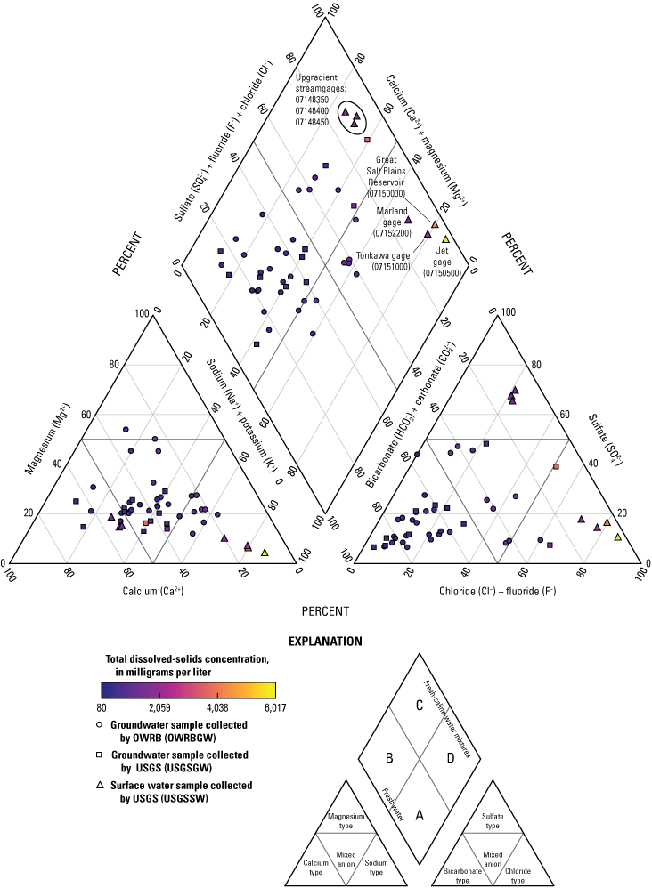
Piper (1944) diagram showing groundwater- and surface-water-quality samples of water produced from the Salt Fork Arkansas River alluvial aquifer, northern Oklahoma, 1950–72 and 2014. USGS, U.S. Geological Survey; OWRB, Oklahoma Water Resources Board. Symbols representing individual samples are shaded to denote relative total dissolved solids concentrations.
The water types of the 37 groundwater samples analyzed for this study (26 samples collected by OWRB, 11 collected by USGS) ranged from bicarbonate as the dominant anion (bicarbonate water type) to chloride as the dominant ion (chloride water type), or a mixture of anions (mixed anion water type) (figs. 12–13). TDS concentrations measured in the groundwater samples were generally lower in the bicarbonate-water type than in the other water types. Of the 37 groundwater samples, 29 were of the bicarbonate water type with calcium, magnesium, or sodium as the dominant cations or characterized by a mixture of cations (mixed cation water type). TDS concentrations of the bicarbonate water type groundwater samples ranged from 86 to 885 mg/L, with a median TDS concentration of 495 mg/L. Groundwater samples from the part of the Salt Fork Arkansas River alluvial aquifer within 3 mi of Pond Creek in Grant County were also of the bicarbonate water type, with major-ion concentrations similar to groundwater samples from most wells along Little Sandy Creek and Sand Creek in Alfalfa County. Bicarbonate water-type samples plot within quadrants A and B of the Piper diagram’s upper diamond on figure 13A. These quadrants represent freshwater types with bicarbonate as the dominant anion and the cations calcium, magnesium, and sodium (plus potassium) representing various percentages of the total ion concentrations. The TDS concentrations were generally the samples representing the highest chloride and mixed-anion water types, which are considered water types indicative of freshwater saline-water mixtures. Chloride or mixed-anion water type samples plot within quadrants C and D of the Piper diagram’s upper diamond (fig. 13). Of 37 groundwater samples, 16 samples were chloride or mixed-anion water types with TDS concentrations ranging from 735 to 1,470 mg/L, and a median TDS concentration of 1,220 mg/L. Major-ion water quality of the Salt Fork Arkansas River at the three USGS surface-water sites was plotted on the Piper diagram as saline end members representing calcium-sulfate and sodium-chloride water types. Shifting the discussion from individual anions and cations to the freshwater and saline water mixtures in the upper diamond, the groundwater-quality samples show generalized mixing from freshwater types in quadrants A and B to the saline end members in quadrants C and D (fig. 13). Quadrants C and D represent groundwater mixtures of different proportions along this mixing region. In general, TDS is higher in groundwater-quality samples approximating saline-end members than in other samples. The triangular anion (ternary) part of the Piper diagram (fig. 13) also illustrates the mixing between freshwater types and saline end-members. Groundwater-quality samples with larger proportions of sulfate and chloride plot closer to the saline-water end members (OWRB, 2018; USGS, 2024).
Surface-water types in the river basin show a distinct difference between sites located upgradient and downgradient from the Great Salt Plains Reservoir (fig. 12). Concentrations of calcium and sulfate were higher upstream from the salt flats, with sodium chloride water types present. Changes in the geology west of the salt flats, where halite and gypsum deposits associated with the Hennessey Group are widespread, create higher saline signatures in the surface-water samples; groundwater-surface interactions are the source of elevated sodium and chloride concentrations in surface water (fig. 9; USACE, 1978; Morton, 1980). At the Great Salt Plains Reservoir, sodium and chloride concentrations are substantially higher than in upstream surface-water samples, which is likely attributable to active exchanges between the salt flats and surface water. Further east, downgradient from the Great Salt Plains Reservoir, the sodium chloride signal decreases but is still much higher than the calcium sulfate signature (fig. 12). In all of the surface-water samples, the magnesium bicarbonate ions are the less dominant ions, as the water is higher in sodium and chloride than most other alluvial aquifers in the State (Dover, 1957; Davis, 1968; Eckenstein, 1994, 1995).
The groundwater well samples generally have less sodium chloride than all of the surface-water samples and higher ionic concentrations of bicarbonate, indicating fresher, less saline groundwater. The groundwater samples collected from wells completed in the alluvial and terrace deposits near the western part of the Great Salt Plains Reservoir were characterized by higher sodium and chloride concentrations and higher calcium and sulfate concentrations compared to groundwater samples collected from wells completed near the eastern part of the study area (fig. 12). In the central to eastern part of the study area, much lower sodium and chloride concentrations and higher bicarbonate concentrations were measured in groundwater samples collected in the alluvium compared to groundwater samples collected from west of the Great Salt Plains Reservoir, indicative of less saline groundwater in this region. In the dune sands north of the salt flats, there are even higher concentrations of bicarbonate than in the central to eastern part of the study area; this observation, combined with the fact that the lowest concentrations of calcium sulfate and sodium chloride measured in the entire aquifer, suggests that the groundwater in the dune sands is the least saline in the study area (fig. 12). The low salinity in the dune sands could be at least partially attributable to percolation of groundwater from the Permian bedrock through the dune sands in the area (Ward, 1961; Davis, 1968). Overall, the groundwater samples collected from wells completed in the alluvium had higher concentrations of sodium and chloride than those collected from wells completed in the terrace deposits. This may be due to the longer residence times the groundwater has with the sediments, possibly allowing for potential chemical interactions that will decrease the concentrations of sodium and chloride from the groundwater that was collected from the wells completed in the terrace deposits. Overall, most of the groundwater samples from the alluvium contain higher concentrations of sodium chloride compared to samples from the terrace deposits because of the longer residence times the groundwater has with the sediments, possibly allowing for potential chemical interactions decreasing the concentrations of sodium chloride in the terrace deposits (fig. 12).
Hydrogeologic Framework
A hydrogeologic framework is a three-dimensional representation of an aquifer and how that aquifer interfaces with surrounding hydrogeologic units at a scale that represents the regional controls on groundwater flow (Smith and others, 2021). The hydrogeologic framework for the alluvium and terrace deposits of the Salt Fork Arkansas River and Chikaskia River alluvial aquifers includes updates to the three-dimensional aquifer extent and potentiometric surface, as well as descriptions of the hydraulic and textural properties of Salt Fork Arkansas River and Chikaskia River alluvial aquifer materials. The hydrogeologic framework was used in the construction of the numerical groundwater-flow model of the Salt Fork Arkansas River and Chikaskia River alluvial aquifers (Smith and Gammill, 2025) described in this report.
Aquifer Extent
Previously published spatial aquifer extents for the Salt Fork Arkansas River and Chikaskia River alluvial aquifers were determined from 1:250,000-scale geologic maps (Stoeser and others, 2005). The spatial aquifer extents for this study were updated by using information from finer (1:100,000) scale geologic maps obtained from OWRB (2022a). The geographic extents of the Salt Fork Arkansas River and Chikaskia River alluvial aquifers (fig. 1) were updated from GMAP Aquifer Study Areas extents available from the OWRB Open Data Portal (OWRB, 2022a) by using information obtained from 1:100,000-scale geologic maps (Miller and Stanley, 2003; Stanley and others, 2003; Stanley and Miller, 2007, 2008). Compared to the coarser scale of the older 1:250,000-scale geologic map of the study area, the finer 1:100,000-scale geologic maps showed a narrower extent of the alluvium and terrace deposits that form the Salt Fork Arkansas River and Chikaskia River alluvial aquifers, and therefore the updated spatial aquifer extents presented in this report are smaller compared to the previously published extents.
For modeling purposes, the updated spatial extents of the Salt Fork Arkansas River and Chikaskia River alluvial aquifers were reduced by removing small tributaries where the width of alluvial materials was less than 2,000 ft, because including these narrow tributaries would contribute negligibly to the characterization of the groundwater system. The updated spatial extents of the Salt Fork Arkansas River and Chikaskia River alluvial aquifers were extended in a few areas where groundwater permits and lithologic logs obtained from well-completion reports (specifically, lithologic logs of the physical characteristics of geologic units observed during the initial drilling of the well [OWRB, 2022a]) indicated that alluvial materials were present in sufficient thickness to allow production of groundwater at a steady rate and, thereby, serve as an economic resource. The largest increase in the spatial extents of the alluvial aquifers was northwest of the Great Salt Plains Reservoir and west of Sand Creek, in an area where the 1:250,000-scale geologic maps showed surficial terrace deposits but the 1:100,000-scale geologic maps did not.
Where present, the top of the Salt Fork Arkansas River alluvial aquifer was defined as the land-surface altitude obtained from a 10-m (horizontal resolution) digital elevation model (DEM) (USGS, 2015), and depressions in the DEM were filled by using the ArcGIS Fill tool (Esri, 2021a). The altitude of the base of the Salt Fork Arkansas River alluvial aquifer, which was equivalent to the bedrock altitude, was contoured at a 25-ft interval from bedrock depths obtained from drillers’ lithologic logs from well-completion reports (OWRB, 2022a), ambient-seismic-method depths (Smith and Gammill, 2025), and test-hole data (Engineering Enterprises, unpub. data, 2021) in addition to data obtained by the USGS from direct-push test holes (fig. 14; USGS, 2024). For each of these data sources, the altitude of the base of the Salt Fork Arkansas River alluvial aquifer was calculated by subtracting the measured bedrock depth from the land-surface altitude. For consistency, the land-surface altitude was obtained from the 10-m DEM, even when the data source provided a land-surface altitude.
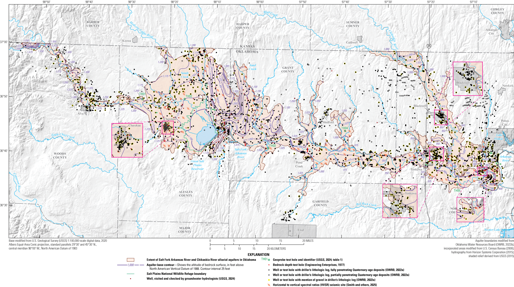
Altitude of the base of the Salt Fork Arkansas River and Chikaskia River alluvial aquifers, northern Oklahoma, decreasing in altitude from west to east.
Top of Bedrock Altitudes From Ambient Seismic Method
Top of bedrock altitudes were estimated by using the horizontal-to-vertical spectral ratio (HSVR) ambient seismic method (Tromino, 2012). The ambient-seismic data were collected by using a Tromino digital seismometer (MOHO S.R.L., Marghera) that gathers ambient seismic shear waves, thereby measuring the frequency and amplitude of shear waves in three axes, two horizontal and one vertical. The shear-wave velocity of unconsolidated alluvial deposits is about half that of consolidated bedrock. The difference in shear-wave velocities in the alluvial deposits and consolidated bedrock cause the horizontal to vertical ratio of the velocities to form a peak from which a measurable resonant frequency of the consolidated bedrock is attained (Tromino, 2012). Bedrock depth is estimated from this resonant frequency according to the following equation from Tromino (2012):
whereZ
is the depth to bedrock, in meters (converted to feet for use in this report);
VS
is the shear-wave velocity of the unconsolidated alluvial deposits, in meters per second (converted to feet for use in this report); and
F0
is the resonant frequency of the consolidated bedrock, in hertz.
In October 2018, ambient-seismic data were collected by using the horizontal-to-vertical spectral ratio method at 99 locations across the Salt Fork Arkansas River alluvial aquifer, with 20 of them being bedrock control points of a known bedrock depth (fig. 14; Smith and Gammill, 2025). The bedrock control points correspond to locations where OWRB lithologic logs were obtained, and from these logs, bedrock depths were spatially determined throughout the extent of the alluvial aquifer. The bedrock depths obtained from the lithologic logs were used as seismometer calibration points. At each location, the digital seismometer was oriented to geographic north and pushed into a flat area of the ground, allowing the stabilizing spikes on the bottom of the unit to firmly anchor into the soil. The instrument was then leveled, calibrated, and set to record for 16 minutes, a timeframe chosen based on the instrumentation guidelines (Koller and others, 2004). The ambient-seismic data were analyzed by using Grilla (Tromino, 2012), a software package provided by the digital seismometer manufacturer. The ambient-seismic data collected by using the horizontal-to-vertical spectral ratio method are available in Smith and Gammill (2025).
Bedrock Depths From Lithologic Logs
Lithologic logs (OWRB, 2022a) were also used to delineate the alluvium and bedrock surface contact of the Salt Fork Arkansas River alluvial aquifer in areas where the bedrock contact depth could be determined. Permian bedrock unit terms were used to identify the four predominant lithologies in the study area: (1) “red beds” (iron-rich reddish sedimentary rocks deposited in hot, oxidizing environments) (Van Houten, 1968); (2) red or gray shale; (3) bedrock; and (4) shale. The bedrock surface was defined by the presence of one of these lithologies overlain by alluvial sand or gravel. The bedrock surface was defined by the occurrence of one of these geology types overlain by alluvial sand or gravel.
Potentiometric Surface and Saturated Thickness
Potentiometric-surface maps show the altitude at which the water level would have stood in tightly cased wells at a specified time; the potentiometric surface is usually contoured or spatially interpolated from synoptic water-table-altitude measurements made in many wells across an aquifer extent. Potentiometric-surface maps are used to indicate the general directions of groundwater flow in an aquifer. Groundwater generally flows perpendicular to potentiometric contours in the direction of decreasing contour altitude (Freeze and Cherry, 1979).
During February 24–28, 2020, a total of 70 synoptic water-table altitudes were measured by using methods described in Cunningham and Schalk (2011) at selected wells in the study area. The wells were generally unused and constructed with steel or slotted polyvinyl chloride (PVC) well casings and a sand-filled annulus. The depth to water was measured, referenced to land surface, and subtracted from the land-surface altitude obtained from a 10-m DEM (USGS, 2015) to determine the water-table altitude referenced to the North American Vertical Datum of 1988. The DEM also was used to obtain water-surface altitudes at selected points along major streams for use as additional control data. A potentiometric surface raster was then interpolated from both sets of water-level altitude data by using inverse-distance-weighted interpolation methods (Esri, 2021b). Potentiometric-surface contours at 25-ft intervals (fig. 15) were derived from the interpolated raster, and the DEM was used to check that contour altitudes remained below land surface altitudes except in areas where flowing wells and wetlands were known to be present. The saturated thickness, as used in this study, is the difference between the water-table altitude and the bedrock (aquifer-base) altitude. The mean saturated thicknesses for the Salt Fork Arkansas River and Chikaskia River alluvial aquifers in February 2020 were about 34.0 and 27.9 ft, respectively. Local flow in the Salt Fork Arkansas River and Chikaskia River alluvial aquifers was generally from topographically high areas toward the Salt Fork Arkansas River and its major tributaries with regional flow in the aquifer generally from west to east (fig. 15). The most notable feature in the potentiometric surface is the potentiometric high associated with the dune sand area northeast of the Great Salt Plains Reservoir. That potentiometric high directs flow west toward Sandy Creek and flowing artesian wells in northeastern Alfalfa County and east toward Sand Creek in Grant County.
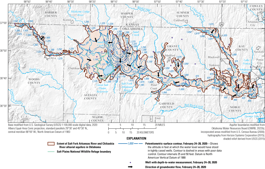
Potentiometric-surface contours and general direction of groundwater flow in the Salt Fork Arkansas River and Chikaskia River alluvial aquifers, northern Oklahoma, February 2020.
Textural and Hydraulic Properties
This section describes (1) textural and aquifer hydraulic properties, such as grain size, distribution, and percent coarse value that were estimated by using lithologic logs, and (2) the spatial distribution of lithologic units to characterize the alluvium and terrace deposits for the Salt Fork Arkansas River alluvial aquifer. The distribution and variability of textural and hydraulic properties of aquifer materials, especially the horizontal hydraulic conductivity, were assumed to be the primary controls on groundwater flow in the Salt Fork Arkansas River and Chikaskia River alluvial aquifers (Sudicky, 1986). Multiple methods were used to estimate the range and central tendency of horizontal hydraulic conductivity values in the aquifer. These methods included in-place estimation in test holes and summarizing data in drillers’ lithologic logs.
Lithologic Logs and Percent Coarse Values
Approximately 3,130 lithologic logs from well-completion reports were analyzed to characterize the alluvium and terrace deposits of the Salt Fork Arkansas River and Chikaskia River alluvial aquifers (OWRB, 2022a). These lithologic logs are submitted to the OWRB by the well drillers and are based on descriptions of the cuttings recorded as the groundwater wells were drilled. Not all groundwater wells have available lithologic logs; only 3,130 lithologic logs from the study area were used to characterize the alluvium and terrace deposits. Lithologic logs based on groundwater wells in Oklahoma have no specified standards related to lithologic descriptions by the well drillers, which leads to many variations in the logs between both the drilling companies and individuals logging the wells. Lithologic logs were downloaded from the OWRB groundwater-well records database (OWRB, 2022a, b).
Variations in the terms used in the lithologic descriptions in the drillers’ logs required simplification and standardization to enable categorization. Most lithologic logs in the OWRB database were from shallow, domestic wells. Limitations of using lithologic logs include possible errors in reported depths identifying transition points between differing lithologies, gaps in spatial locations of wells, and inconsistent lithologic descriptions. Records with obvious errors were corrected to extract as much data as possible (such as logs with missing or mislabeled sections that still provided useful data about some of the geologic units in the study area). In some cases, an entire log was omitted from the analysis if it was substantially incomplete and lacked usable information.
Hydraulic Conductivity Estimation Based on Lithologic Categorization
The hydraulic conductivity of the Salt Fork Arkansas River alluvial aquifer was determined by applying a percent coarse material multiplier (table 8) to lithology-specific depth intervals within each compiled lithologic log based on lithologic category. There are many variations in categories of lithologic logs, but most lithologic categories defined by drillers on the lithologic logs include some combination of gravel, sand, and clay. Most categories vary widely among each driller’s log depending upon the driller doing the drilling analysis. To standardize and simplify the lithologic logs, the lithologic descriptions were reclassified into five categories that were used to estimate the percentage of coarse material range of each depth interval. Lithology was categorized into clay and silt, fine sand, medium sand, coarse sand, and fine gravel. A percentage of coarse material values (ranging from 0 to 100 percent) based on the midpoint size range of each category was assigned to each lithologic-log depth interval based on the lithologic category assigned (table 8; Wentworth, 1922; Guy, 1969; Mashburn and others, 2018).
Table 8.
Percentage of coarse-material multiplier values for the generalized lithologic categories used to obtain horizontal hydraulic conductivity values for the Salt Fork Arkansas River and Chikaskia River alluvial aquifers, northern Oklahoma.Size categories for the different lithologic categories are described in Wentworth (1922) and Guy (1969).
The hydraulic properties of the Salt Fork Arkansas River and Chikaskia River alluvial aquifer materials were estimated using techniques to simplify the lithologic description as described in Mashburn and others (2018) The percentage of coarse material value for each lithologic log was then used to estimate and spatially interpolate the hydraulic properties of the Salt Fork Arkansas River alluvial aquifer materials.
A percentage of coarse material value of 0 percent represents silt and clay size material, whereas a value of 100 percent represents fine gravel size material. If there was
-
• 0–20 percent coarse material, the given section of the lithologic log was classified as clay and silt and assigned a percent-coarse multiplier value of 10 (table 8);
-
• 21–40 percent coarse material, the given section of the lithologic log was classified as fine sand and assigned a percent-coarse multiplier value of 30 (table 8);
-
• 41–60 percent coarse material, the given section of the lithologic log was classified as medium sand and assigned a percent-coarse multiplier value of 50 (table 8);
-
• 61–80 percent coarse material, the given section of the lithologic log was classified as coarse sand and assigned a percent-coarse multiplier value of 70 (table 8); and
-
• 81–100 percent coarse material, the given section of the lithologic log was classified as fine gravel and assigned a percent-coarse multiplier value of 90 (table 8).
The percentage of coarse material value for each lithologic-log depth interval was determined as the thickness-weighted mean of the percentage of coarse material values assigned to the lithologic categories in each log.
A horizontal hydraulic conductivity of 0.1 foot per day (ft/d) was assigned to the clay and silt standardized category, and a horizontal conductivity of 100.1 ft/d was assigned to the fine gravel standardized category based on the thickness-weighted mean horizontal hydraulic conductivity values estimated for each lithologic category (Heath, 1983; Mashburn and others, 2018). This range of categories spans the expected grain sizes in the Salt Fork Arkansas River alluvium and terrace deposits. By assuming that a horizontal hydraulic conductivity of 0.1 ft/d and a percentage of coarse material multiplier of 10 represents the clay and silt standardized category and that a horizontal hydraulic conductivity of 100 ft/d and a percentage of coarse material multiplier of 90 represents the fine gravel standardized category, as well as that the relation between the two properties is linear, the mean horizontal hydraulic conductivity for the aquifer material was calculated by using the following equation modified from Ellis and others (2017):
whereKh
is the thickness-weighted mean horizontal hydraulic conductivity, in feet per day;
t
is the thickness, in feet, of the lithologic log interval; and
Ps
is the percentage of coarse material value assigned to the lithologic log interval.
The frequency distribution of horizontal hydraulic conductivity (fig. 16) was determined by using equation 2 for lithologic logs with a minimum thickness of 15 ft, which was thought to be the minimum thickness that could support productive wells. Observations used to calculate hydraulic conductivities were obtained from 2,386 driller’s lithologic logs and 5 core samples. The mean hydraulic conductivity is 32.1 ft/d for the lithologic log samples (fig. 16). Figure 16A compares the hydraulic conductivity estimates derived from the core data versus the lithologic log data. The core samples indicated a mean hydraulic conductivity of about 32.1 ft/d. The core samples were not included in figure 16B because of the small sample size relative to the lithologic log sample size. Most hydraulic conductivity values estimated for the Salt Fork Arkansas River alluvial aquifer were in the range of 16–50 ft/d (fig. 16). The increased frequency of lithologic logs with horizontal hydraulic conductivity at 0–4 ft/d is mostly caused by an abundance of logs in which the lithology was fine throughout the vertical profile before terminating at bedrock at a relatively shallow depth (less than 25 ft).
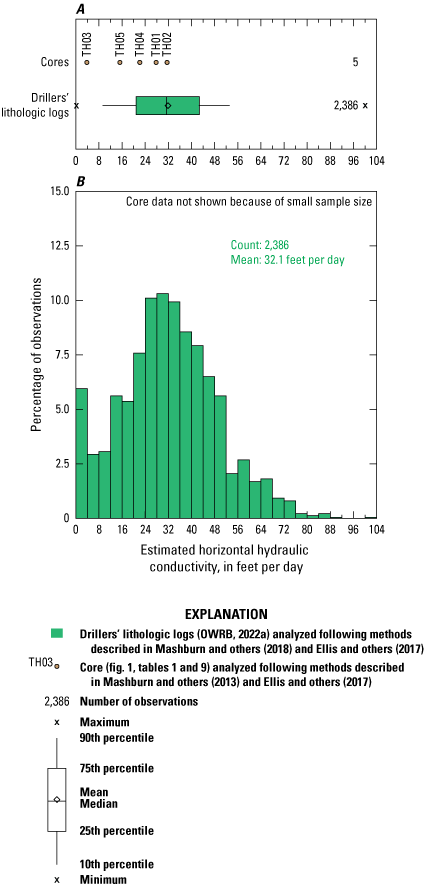
Frequency distribution of hydraulic conductivity values estimated from Oklahoma Water Resources Board (OWRB, 2022a) lithologic logs for wells and core test holes in the Salt Fork Arkansas River and Chikaskia River alluvial aquifers, northern Oklahoma.
Core Sample Description
Five core sediment samples were collected across the Salt Fork Arkansas River alluvial aquifer (TH01-TH05 in fig. 1) at locations where a Geoprobe hydraulic profiling tool was used alongside the direct push coring to log electrical conductivity, pressure (corrected for hydrostatic gradient when saturated), and flow rate with depth (Geoprobe Systems, 2015). By using the Direct Imaging Viewer software by Geoprobe, the hydraulic conductivity could be calculated at different depths in each test hole. To accurately interpret the lithology of the sediments with depth, the ratio of the measured flow rate to the corrected pressure was used in the calculation, as was the Hydraulic Profiling Tool (HPT) pressure and electrical conductivity (Geoprobe Systems, 2020). A conventional HPT log typically includes both HPT pressure and electrical conductivity ranges that the software will use to calculate hydraulic conductivity, which will then show an increase in hydraulic conductivity with increasing grain size (McCall, 2010). Ten HPT test holes were planned in conjunction with the project. The study area was determined to have too much clay and salt that adversely affected HPT equipment functionality, with issues such as clay clogging the probe and high salt content affecting electrical conductivity readings. These continual malfunctions led to the abandonment of the HPT part of the analysis and exclusive reliance on the five cores and lithological logs.
The sediment cores were obtained by using a 66-DT direct-push Geoprobe (Geoprobe Systems, 2007). Sediment cores were collected from land surface to the point of refusal, which was assumed to be the sediment-bedrock contact. Sediment cores were collected in 2.25-in.-diameter by 48-in.-long plastic sleeves. The cores were processed at the USGS office in Oklahoma City, Okla. Two parallel cuts along the length of the core sleeve were made with parallel, double-hooked blades to expose the sediment core for accurate descriptions of color and texture. The sediment cores were described increments of 1-in., and changes in grain size, sorting, and Munsell (1912) color were noted (table 9). On the basis of their lithologic descriptions, each sediment core interval was assigned to one of the five lithologic categories from the lithologic log standardization. A mean horizontal hydraulic conductivity was determined based on the relative proportions of the different lithologic categories found in each core. Some of the maximum core depths did not correlate with the depth of the core interval descriptions because either the core was compressed during processing or the core sleeve was damaged, compromising the sample.
Table 9.
Physical and lithologic descriptions of five core samples from the Salt Fork Arkansas River alluvial aquifer (Munsell, 1912).[ft, foot; DD, decimal degrees; NAD 83, North American Datum of 1983]
| Core interval (in 4 ft sections) | Description | Munsell color (Munsell, 1912) |
Estimated Kh |
|---|---|---|---|
| 0–4 | Loose sand, very fine and fine sand, about 20 percent silty clay | 5 YR 4/3 | 27.6 |
| 4–8 | Very fine and fine sand, well sorted, moist. Sandy shale, overall about 80 percent silty clay/shale | 5 YR 4/6 | 27.6 |
| 8–12 | Sandy silt and clay, no bedding, about 5 percent gravel | 5 YR 4/6 | 27.6 |
| 12–16 | Dry hard poorly sorted sand and silt | 5 YR 4/4 | 27.6 |
| 16–20 | Clay some silt brittle well sorted. Zones of grey-white clay to bedrock. | 5 YR 7/4 | 27.6 |
| 0–4 | Very fine sand, well sorted | 5 YR 6/4 | 31.4 |
| 4–8 | Sand that ranges from silt-size particles to very fine sand. Poorly sorted to well sorted; soft and moist | 5 YR 6/4 | 31.4 |
| 8–12 | Mix of sand with silt and clay; well sorted and moist | 7.5 YR 7/3 | 31.4 |
| 12–16 | Sandy clay some pebbles, some silt. Mostly sand poorly sorted | 7.5 YR 7/2 | 31.4 |
| 16–20 | Salt-mostly clay and silt some sand | 7.5 YR 6/4 | 31.4 |
| 20–24 | About 50 percent sand about 50 percent clay, subangular with some small pebbles | 2.5 YR 7/1 | 31.4 |
| 0–4 | Silt and very fine sand to silt and clay, well sorted. | 5 YR 4/4 | 3.7 |
| 4–8 | Silt and clay hard and dry | 5 YR 4/6 | 3.7 |
| 8–12 | Clay hard, well sorted | 5 YR 4/2 | 3.7 |
| 12–16 | Clay, well sorted. | 5 YR 3/2 | 3.7 |
| 16–20 | Clay hard, no bedding | 5 YR 3/2 | 3.7 |
| 20–24 | Clay hard, no bedding | 2.5 YR 6/1 | 3.7 |
| 24–28 | Clay hard, no bedding | 5 YR 5/1 | 3.7 |
| 0–4 | Sand to silt and clay, well sorted | 5 YR 3/3 | 22.0 |
| 4–8 | Very fine sand to mostly sand with some clay | 7.5 YR 4/3 | 22.0 |
| 8–12 | Silt and clay well blended | 2.5 YR 4/6 | 22.0 |
| 12–16 | Very fine sand and clay/silt fining upward sequence | 2.5 YR 3/6 | 22.0 |
| 0–4 | Mostly clay and sand near the top, about 20 percent fine gravel, some sand | 7.5 YR 5/4 | 15.1 |
| 4–8 | About 90 percent clay and silt, about 10 percent fine sand, and gypsum/salt | 7.5 YR 3/3 | 15.1 |
| 8–12 | About 95 percent clay and silt, about 5 percent fine sand and gravel, gypsum/salt present | 7.5 YR 2.5/3 | 15.1 |
| 12–16 | About 95 percent clay and silt, about 5 percent fine sand and gravel, gypsum/salt present | 7.5 YR 2.5/3 | 15.1 |
| 16–20 | About 95 percent clay and silt, about 5 percent fine sand and gravel, gypsum/salt present | 7.5 YR 2.5/3 | 15.1 |
The five sediment cores were mostly composed of very fine to fine sands, clays, and silts (table 9) (USGS, 2021). Numerous salt layers were distributed throughout each sediment core. Most of the sediment-core layers were well sorted, with no signs of bedding evident, and all of the cores were compressed because of the pliable nature of the alluvial sediments. The Munsell Coloring System describes the color of sediments on the basis of hue, value, and chroma (Munsell, 1912). Most coloring across the study area ranges from 5 to 7.5 YR, meaning 5 to 7.5 parts yellow to 1 part red, respectively (table 9). Hydraulic conductivities were calculated for each core by using the same method described in the “Hydraulic Conductivity Estimation Based on Lithologic Categorization” section of this report. Among all sediment core samples, the maximum computed hydraulic conductivity was 31.4 ft/d and the minimum was 3.74 ft/d (table 9), which is consistent with the hydraulic conductivity described by Eckenstein (1995) for wells in the Salt Fork Arkansas River alluvial aquifer.
Textural and Hydraulic Properties From Other Reports
No sites suitable for multiwell aquifer tests were found in the Salt Fork Arkansas River or Chikaskia River alluvial aquifers. Reed and others (1952) estimated specific yield from nine multiwell aquifer tests of about 0.8- to 1.0-day duration in the Cimarron Terrace aquifer, which is the nearest alluvial aquifer south of the study area. The specific-yield estimates for the Cimarron Terrace aquifer ranged from 0.018 to 0.131 and averaged 0.065 (Reed and others, 1952). The mean specific-yield value from Reed and others (1952) was less than the specific-yield values used in calibrated models for other alluvial aquifers in Oklahoma; however, the range of specific-yield values from Reed and others (1952) included the specific-yield values used in calibrated models for other alluvial aquifers in Oklahoma (Smith and others, 2017, 2021; Ellis and others, 2020; Rogers and others, 2023).
Vertical anisotropy (ratio of horizontal to vertical hydraulic conductivity) and specific storage values have not previously been measured in the Salt Fork Arkansas River or Chikaskia River alluvial aquifers and for this assessment were assumed to be comparable to those used in simulations of water availability in the nearby Salt Fork Red River aquifer (Smith and others, 2021), which used vertical anisotropy and specific storage values of 10.0 and 1×10⁻⁵ ft-1, respectively. Values for vertical anisotropy and specific storage from Smith and others (2021) were each within the ranges suggested by Domenico and Schwartz (1998) for unconsolidated aquifer materials like those of the Salt Fork Arkansas River alluvial aquifer.
Conceptual Groundwater-Flow Model and Water Budget
A conceptual groundwater-flow model is a simplified description (or diagram) of the major inflow and outflow sources (hydrologic boundaries) of a groundwater-flow system and includes a water-budget accounting of the estimated mean flows (water-budget components) from those sources for a specified period (Harbaugh, 1990). A conceptual groundwater-flow model (hereinafter referred to as the “conceptual model”) for the Salt Fork Arkansas River and Chikaskia River alluvial aquifers was developed to guide and constrain the construction and calibration of a numerical groundwater-flow model (hereinafter referred to as the “numerical model”) for the aquifers. The conceptual-model water budget (table 10; fig. 17A) was used to estimate mean annual inflows to, and outflows from, the Salt Fork Arkansas River and Chikaskia River alluvial aquifers for the 1980–2020 study period. The conceptual-model water budget included a subaccounting of mean annual inflows and outflows for reaches of the Salt Fork Arkansas River alluvial aquifer upgradient and downgradient from the Great Salt Plains Reservoir dam and the Chikaskia River alluvial aquifer (fig. 1) to allow more detailed comparisons of groundwater flows in subareas with different mean annual precipitation values and depositional regimes. The conceptual-model (and numerical-model) aquifer area totaled 512,808 acres (table 10).
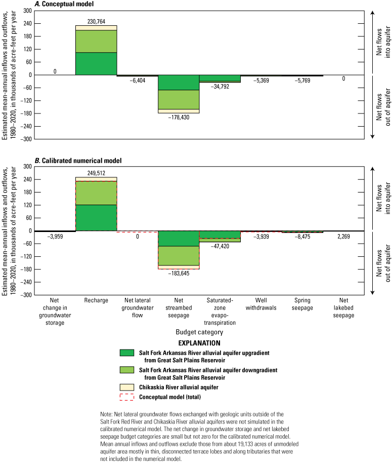
Estimated mean annual inflows and outflows by water-budget component for the A, conceptual model, and B, calibrated numerical model of the Salt Fork Arkansas River and Chikaskia River alluvial aquifers, northern Oklahoma, 1980–2020.
Table 10.
Conceptual-model water budget of estimated mean annual inflows and outflows for simulated wetland areas within the Salt Fork Arkansas River and Chikaskia River alluvial aquifers, northern Oklahoma, 1980–2020.[All water-budget component values are in units of acre-feet per year. Totals may not equal sum of components because of independent rounding. Net streambed seepage, net lateral groundwater flow, and net change in groundwater storage represent the net effect of aquifer inflows and outflows. NWI, National Wetlands Inventory; OWRB, Oklahoma Water Resources Board; in/yr, inch per year. --, not quantified or not applicable]
| Descriptor | Salt Fork Arkansas River alluvial aquifer upgradient from Great Salt Plains Reservoir | Salt Fork Arkansas River alluvial aquifer downgradient from Great Salt Plains Reservoir | Chikaskia River alluvial aquifer | Total | Percentage of water budget | Uncertainty | Notes |
|---|---|---|---|---|---|---|---|
| Modeled area, in cells | 15,802 | 15,768 | 3,333 | 34,903 | -- | -- | |
| Modeled area, in acres | 232,169 | 231,669 | 48,970 | 512,808 | -- | -- | |
| Modeled area, in percent | 45.3 | 45.2 | 9.5 | 100.0 | -- | -- | |
| Wetland area, in acres | 21,748 | 3,945 | 466 | 26,160 | -- | -- | Sum of “Freshwater Emergent Wetland,” “Riverine,” “Lake,” and “Other” categories from NWI (U.S. Fish and Wildlife Service, 2017). |
| Wetland area, in percent | 83.1 | 15.1 | 1.8 | 100.0 | -- | -- | Same as above. |
| Recharge | 104,476 | 104,251 | 22,036 | 230,764 | 100.0 | Medium | 5.4 in/yr or 16.3 percent of mean annual precipitation (table 3) |
| Net change in groundwater storage | -- | -- | -- | -- | -- | Low | Assumed to be a negligible part of water budget |
| Total inflow | 104,476 | 104,251 | 22,036 | 230,764 | 100.0 | -- | |
| Net streambed seepage | 70,571 | 89,774 | 18,084 | 178,430 | 77.3 | Medium | Estimated from base-flow data at streamgages (tables 4, 5) |
| Saturated-zone evapotranspiration | 28,925 | 5,247 | 620 | 34,792 | 15.1 | High | 1.33 ft/yr (Rogers and others, 2023) times riverine- and lake-type wetland area of 26,160 acres (U.S. Fish and Wildlife Service, 2017) |
| Well withdrawals | 1,971 | 2,956 | 442 | 5,369 | 2.3 | Medium | From OWRB reported groundwater-use data (tables 6, 7) |
| Net lateral groundwater flow | 396 | 3,668 | 2,340 | 6,404 | 2.8 | High | Unknown; assumed to be a negligible part of water budget; calculated as balance of water budget |
| Spring seepage | 2,612 | 2,606 | 551 | 5,769 | 2.5 | High | Unknown; assumed to be about 2.5 percent of water budget |
| Net lakebed seepage | -- | -- | -- | -- | -- | High | Unknown; assumed to be a negligible part of water budget |
| Total outflow | 104,476 | 104,251 | 22,036 | 230,764 | 100.0 | -- |
Varying levels of uncertainty are associated with the estimated mean annual flows to hydrologic boundaries of the conceptual model. Where possible, estimated mean annual flows to hydrologic boundaries were based on field measurements from the study area made during the study period. In cases where field measurements were unavailable or outside the scope of this study, estimated flows in the conceptual model were assumed to be analogous to those of published conceptual models from similar aquifers in Oklahoma (Ryter and Correll, 2016; Ellis and others, 2017, 2020; Smith and others, 2017, 2021; Ellis, 2018; Rogers and others, 2023). The “notes” section of table 10 summarizes data sources and assumptions used to construct the conceptual-model water budget for the Salt Fork Arkansas River and Chikaskia River alluvial aquifers.
Water-Budget Components
Water-budget components in the conceptual model summarize actual inflows and outflows of water across the hydrologic boundaries of the aquifer. Water-budget components that act as both inflows and outflows may be referred to as “net inflows” or “net outflows” depending on which flow component dominates.
Recharge
Recharge is the predominant source of water in the Salt Fork Arkansas River and Chikaskia River alluvial aquifers. Recharge is defined in this report as the amount of precipitation and applied irrigation water that infiltrates from the land surface through the unsaturated zone and reaches the groundwater level over a given time. This definition of recharge includes irrigation return flows to groundwater. Other processes, such as stream seepage or lateral groundwater flow from adjacent hydrogeologic units, are not considered recharge and are accounted for separately in the conceptual-model water budget. Recharge rates are controlled by many factors, including precipitation rate, land-surface gradient, soil and sediment permeability, evapotranspiration rates, and vegetation cover type (citation needed). Although recharge rates are difficult to measure because of high spatial and temporal variability, methods involving environmental tracers, physical measurements, streamflow-hydrograph techniques, and computer codes can be used to estimate recharge rates. For this study, a groundwater-hydrograph-based water-table-fluctuation (WTF) method (Healy and Cook, 2002) was used to estimate localized recharge rates for 1981–95 and 2019–21, and a code-based water-balance-estimation technique (Westenbroek and others, 2010) was used to estimate spatially distributed recharge rates for the 1980–2020 study period.
Groundwater Level Fluctuations
Historical and active groundwater well sites were used for monitoring; each well was instrumented with a vented pressure transducer and set to record at 1-hour or 30-minute intervals. Two historical continuous recorder groundwater wells were set to record depth-to-water observations at 1-hour intervals. The first historical continuous recorder groundwater well, Alva near Alva, Okla. (USGS station 365143098404201), was active from July 1980 to September 1995. The second historical continuous recorder groundwater well, Burl near Burl, Okla. (USGS station 365342098175301) was active from August 1983 to May 1990. Two continuous recorder groundwater wells monitoring the Salt Plains National Wildlife Refuge recorded depth-to-water observations at 30-minute intervals from October 2013 to present (2025): well GSP1 (USGS station 364821098144901) and well GSP2 (USGS station 364831098120201) (fig. 1, table 11).
Table 11.
Groundwater well data-collection stations in and near the Salt Fork Arkansas River and Chikaskia River alluvial aquifers, northern Oklahoma.[U.S. Geological Survey (USGS, 2024) data can be accessed using the 15-digit station number or other identifier. M/D/Y, month/day/year; NAD 83, North American Datum of 1983; NAVD 88, North American Vertical Datum of 1988; --, unknown or not applicable, SFR2, Streamflow-Routing package; WTF, water-table-fluctuation method]
| Station name | Station number | Other identifier (fig. 1) | Latitude (decimal degrees NAD 83) | Longitude, (decimal degrees NAD 83) | County | Period of record (may contain gaps) (M/D/Y) |
Land-surface altitude, (feet above NAVD 88) |
Well or hole depth (feet) | Use in numerical groundwater-flow model | |
|---|---|---|---|---|---|---|---|---|---|---|
| Begin | End | |||||||||
| 27N-11W-12 BCB 1 SFAR01A | 365013098202902 | W01 | 36.8369 | −98.3414 | Alfalfa | 4/10/2019 | 3/7/2022 | 1,177 | -- | -- |
| 26N-09W-02 AAD 1 SFAR02 | 364555098074101 | W02 | 36.7654 | −98.1282 | Alfalfa | 4/11/2019 | 3/7/2022 | 1,128 | 33 | Recharge (WTF) |
| 26N-07W-11 CCD 1 SFAR03 | 364422097553901 | W03 | 36.7395 | −97.9275 | Grant | 4/11/2019 | 3/7/2022 | 1,092 | 75 | Recharge (WTF) |
| 26N-03W-33 DAA 1 SFAR04 | 364112097310101 | W04 | 36.6867 | −97.5171 | Grant | 4/12/2019 | 6/16/2021 | 1,000 | 39.4 | Recharge (WTF) |
| 25N-02E-15 AAD 1 SFAR05A | 363856097040401 | W05 | 36.6488 | −97.0677 | Kay | 5/1/2019 | 3/7/2022 | 956 | -- | Recharge (WTF) |
| 27N-09W-09 BBA 2 SFAR06 | 365025098104301 | W06 | 36.8403 | −98.1786 | Alfalfa | 5/2/2019 | 3/7/2022 | 1,226 | 29 | -- |
| 27N-13W-11 CDB 1 SFAR07 | 364947098341401 | W07 | 36.8297 | −98.5705 | Woods | 5/3/2019 | 3/7/2022 | 1,273 | 18.3 | Recharge (WTF) |
| 28N-14W-20 CBA 1 SFAR08 | 365327098440001 | W08 | 36.8908 | −98.7333 | Woods | 5/1/2020 | 9/7/2021 | 1,368 | 30.3 | -- |
| 28N-14W-35 BCC 1 Alva GW Well | 365143098404201 | Alva | 36.8639 | −98.6823 | Woods | 7/30/1980 | 9/29/1995 | 1,360 | 54 | Recharge (WTF) |
| 28N-11W-27 DAD 1 Burlington GW Well | 365342098175301 | Burl | 36.8745 | −98.3604 | Alfalfa | 8/25/1983 | 5/20/1990 | 1,185 | 36 | Recharge (WTF) |
| 27N-09W-19 AAD 1 GSP Refuge GW WELL 2 | 364831098120201 | GSP2 | 36.8086 | −98.2007 | Alfalfa | 10/1/2013 | Present | 1,136 | 22.5 | -- |
| 27N-09W-24 AAC 1 GSP Refuge GW WELL 1 | 364821098144901 | GSP1 | 36.8058 | −98.2471 | Alfalfa | 10/1/2013 | Present | 1,143 | 29.2 | -- |
| 27N-12W-12-BCB 1 (SFAR HPTCo 1) | 365010098270001 | TH01 | 36.836 | −98.45 | Alfalfa | -- | -- | -- | 21.1 | Hydraulic properties and aquifer base |
| 27N-10W-04-CCD 1 (SFAR HPTCo 2) | 365025098170801 | TH02 | 36.8405 | −98.2857 | Alfalfa | -- | -- | -- | 22.6 | Hydraulic properties and aquifer base |
| 26N-07W-28-DCC 1 (SFAR HPTCo 3) | 364142097572401 | TH03 | 36.6951 | −97.9568 | Grant | -- | -- | -- | 38.4 | Hydraulic properties and aquifer base |
| 26N-04W-08-BBB 1 (SFAR HPTCo 4) | 364509097393601 | TH04 | 36.7526 | −97.6602 | Grant | -- | -- | -- | 21.8 | Hydraulic properties and aquifer base |
| 25N-01E-32-CDC 1 (SFAR HPTCo 5) | 363538097132001 | TH05 | 36.594 | −97.2225 | Kay | -- | -- | -- | 39.6 | Hydraulic properties and aquifer base |
| 28N-14W-35 BCC 1 Alva GW Well | 365143098404201 | Alva | 36.8639 | −98.6823 | Woods | 1/5/1980 | 10/3/1995 | 1,361 | 54 | Calibration |
| 27N-11W-23 ABD 1 | 364837098205501 | 9006 | 36.8103 | −98.349 | Alfalfa | 1/28/1980 | 1/14/2015 | 1,180 | 41 | Calibration |
| 26N-05W-31 ADA 1 | 364133097460901 | 9431 | 36.6925 | −97.7695 | Grant | 1/31/1980 | 1/8/2018 | 1,040 | 51 | Calibration |
| 25N-01W-08 BBA 1 | 364001097200001 | 9506 | 36.6653 | −97.3337 | Kay | 2/1/1980 | 2/25/1997 | 962 | -- | Calibration |
| 29N-09W-18 CDD 1 | 365916098125001 | 9009 | 36.9878 | −98.2142 | Alfalfa | 1/29/1980 | 8/27/1993 | 1,225 | 35 | Calibration |
| 27N-09W-19 AAD 1 GSP Refuge GW WELL 2 | 364831098120201 | GSP2 | 36.8086 | −98.2007 | Alfalfa | 9/9/2013 | 6/15/2020 | 1,136 | 22.5 | Calibration |
Eight additional groundwater wells completed in the Salt Fork Arkansas River alluvial aquifer were selected on the basis of their distance from streams, varied geologic setting, and availability for use and were instrumented with Level TROLL 500 vented pressure transducers (In-Situ, Inc., 2023) set to continuously record the depth to water every 30 minutes. Depth-to-water observations were recorded during the following periods:
-
• April 2019 to March 2022 at wells W01 (USGS station 365013098202902), W02 (USGS station 364555098074101), and W03 (USGS station 364422097553901).
-
• April 2019 to June 2021 at well W04 (USGS station 364112097310101).
-
• May 2019 to March 2022 at wells W05 (USGS station 363856097040401), W06 (USGS station 365025098104301), and W07 (USGS station 364947098341401).
-
• May 2020 to September 2021 at well W08 (USGS station 365327098440001); the continuous recorder installed at this well was discontinued after only 17 months of operation because of frequent equipment damage by wildlife.
Hydrologic stressors can cause groundwater-level fluctuations on a spatial and temporal basis (Freeze and Cherry, 1979). The primary hydrologic stressors that affect groundwater-level fluctuations in an alluvial aquifer include precipitation, groundwater/surface-water interactions, groundwater withdrawals, evapotranspiration, and streamflow. Similar groundwater-level fluctuations were observed at the eight instrumented groundwater wells in response to precipitation and because of groundwater/surface-water interactions. During spring and summer, declining groundwater levels are primarily associated with seasonally higher rates of groundwater withdrawals for irrigation during the growing season from April through October; groundwater-level declines caused by evapotranspiration are also highest in spring and summer. Variations in streamflow in response to periods of stormwater runoff and periods of drought can cause groundwater levels to fluctuate appreciably in alluvial aquifers (Freeze and Cherry, 1979).
Water-Table-Fluctuation Method
The WTF method (Healy and Cook, 2002) was the primary method used to estimate recharge to the Salt Fork Arkansas River and Chikaskia River alluvial aquifers. The WTF method assumes that rises in groundwater levels in unconfined aquifers that occurred during a relatively short period (hours to a few days) can be attributed to recharge arriving at the saturated zone following a period of precipitation. The WTF method is most appropriately applied to groundwater wells in areas where the groundwater level is shallow, and hydrographs show sharp increases in groundwater levels after precipitation (Healy and Cook, 2002). The WTF method cannot account for a steady rate of recharge or recharge from sources other than precipitation. Annual recharge (R), in inches per year, was estimated by using the following equation:
whereSy
is the specific yield (dimensionless);
Δh
is the rise in groundwater-level altitude, in inches; and
Δt
is the change in time, in years.
Water-level hydrographs from seven USGS continuous-recorder wells (Alva, Burl, W02, W03, W04, W05, and W07; USGS [2024], fig. 1, table 11) in the Salt Fork Arkansas River alluvial aquifer were used to estimate annual recharge for 1981–95 and 2019–21. Wells Alva, Burl, and W07 (fig. 18A–C) were upgradient from the Great Salt Plains Reservoir, whereas wells W02, W03, W04, and W05 (fig. 18D–G) were downgradient from the Great Salt Plains Reservoir (fig. 1, table 11). The water-level hydrographs from other continuous-recorder wells in the Salt Fork Arkansas River alluvial aquifer were not analyzed because they were affected by surface-water seepage (wells W01, W06, and GSP1, fig. 18H–J), did not show sharp water-level rises (well W08, fig. 18K), or were affected by nearby groundwater withdrawals (well GSP2, fig. 18L). Daily precipitation data were obtained from the climate station with at least 96 percent precipitation-data coverage nearest to each continuously monitored well (fig. 2; National Centers for Environmental Information, 2022); those precipitation data were summed for each year of the analysis period (table 3). A specific yield of 0.12 for wells upgradient from the Great Salt Plains Reservoir and 0.065 for wells downgradient from the reservoir were assumed from aquifer tests in the nearby Cimarron Terrace aquifer (Reed and others, 1952); a larger specific yield (near the upper end of those measured by Reed and others [1952]) was used for the wells upgradient from the Great Salt Plains Reservoir because of the predominance of windblown (presumably well-sorted) dune sand (fig. 9) in the upgradient part of the aquifer (table 12). The annual recharge rate, in inches per year, was calculated as the product of the specific yield and the sum of annual water-level rises, in inches. The annual recharge estimates ranged from 0.0 in. (0.0 percent of the station’s annual precipitation) to 12.1 in. (26.5 percent of the station’s annual precipitation) (table 12).
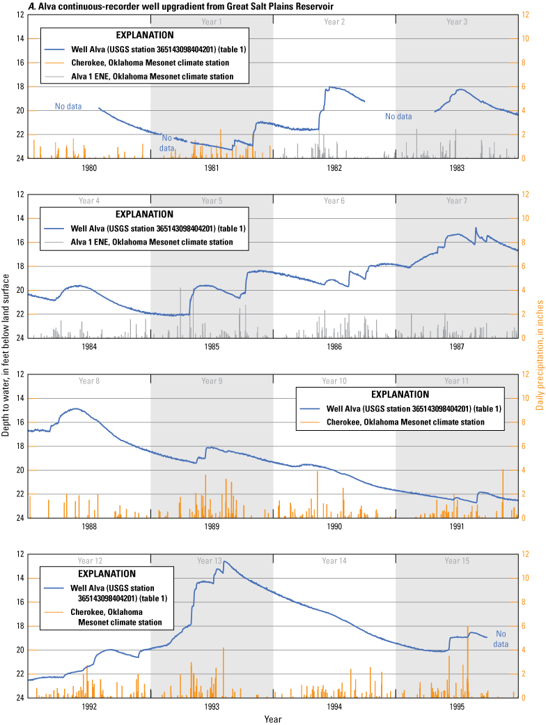
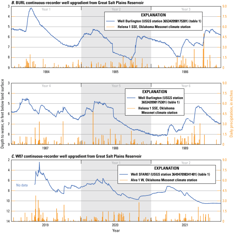
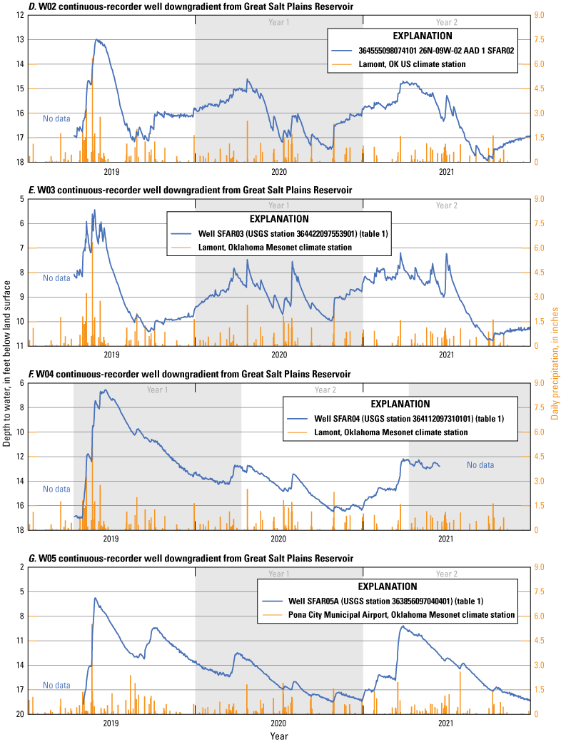
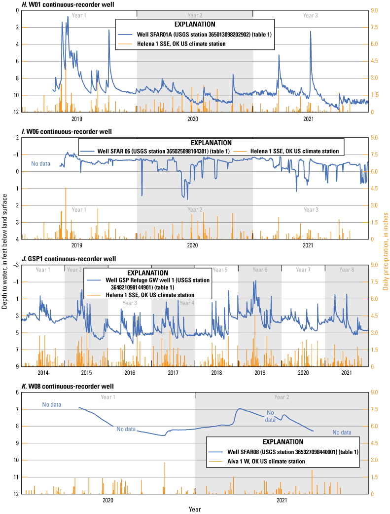
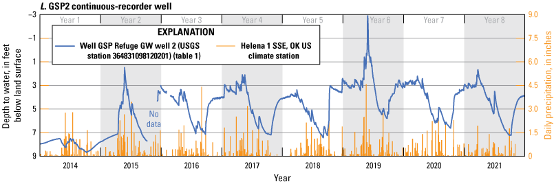
Daily precipitation and depth to water in U.S. Geological Survey (USGS) continuous water-level recorder wells completed in the Salt Fork Arkansas River and Chikaskia River alluvial aquifers, northern Oklahoma, 1981–95 and 2019–21.
Table 12.
Summary of recharge amounts estimated using the water-table-fluctuation method for the Salt Fork Arkansas River alluvial aquifer, northern Oklahoma, 1981–95 and 2019–21.[NCEI, National Centers for Environmental Information. Dates in month, day, year format. Continuous water-level recorder wells W01, W06, W08, GSP1, and GSP2 were not suitable for analysis with the water-table-fluctuation method. E, base-10 exponent (for example, 6.5E-02 equals 6.5×10⁻²); --, not quantified or not applicable]
| Descriptor | U.S. Geological Survey continuous water-level-recorder well (fig. 1; table 11) | ||||||
|---|---|---|---|---|---|---|---|
| Upgradient from Great Salt Plains Reservoir | Downgradient from Great Salt Plains Reservoir | ||||||
| Alva | Burl | W07 | W02 | W03 | W04 | W05 | |
| Mean annual precipitation 1980–2020, in inches, northern Oklahoma (NCEI, 2022; table 3) | 31.4 | 31.4 | 31.4 | 35.1 | 35.1 | 35.1 | 35.1 |
| Climate station (fig. 2, table 2) | ALE, CHE | HEL | ALW | LAM | LAM | LAM | PON |
| Specific yield (dimensionless; values obtained from Reed and others [1952, table 12]) | 1.2E-01 | 1.2E-01 | 1.2E-01 | 6.5E-02 | 6.5E-02 | 6.5E-02 | 6.5E-02 |
| Year 1, beginning date | 1/1/1981 | 1/1/1984 | 1/1/2020 | 1/1/2020 | 1/1/2020 | 4/12/2019 | 1/1/2020 |
| Station annual precipitation, in inches | 30.2 | 21.9 | 30.7 | 31.4 | 31.4 | 45.6 | 29.7 |
| Sum of water-level rises, in feet | 2.9 | 4.0 | 4.9 | 7.1 | 9.9 | 15.5 | 7.8 |
| Recharge, in inches per year | 4.2 | 5.8 | 7.1 | 5.5 | 7.7 | 12.1 | 6.1 |
| Recharge, percent of annual precipitation | 13.8 | 26.3 | 23.0 | 17.7 | 24.6 | 26.5 | 20.5 |
| Recharge, in inches per year, normalized to mean annual precipitation 1980–2020 | 4.3 | 8.3 | 7.2 | 6.2 | 8.6 | 9.3 | 7.2 |
| Year 2, beginning date | 11/1/1982 | 1/1/1985 | 1/1/2021 | 1/1/2021 | 1/1/2021 | 4/12/2020 | 1/1/2021 |
| Station annual precipitation, in inches | 25.6 | 30.2 | 23.2 | 23.3 | 23.3 | 30.9 | 25.6 |
| Sum of water-level rises, in feet | 3.9 | 3.4 | 2.5 | 4.2 | 7.2 | 8.1 | 10.7 |
| Recharge, in inches per year | 5.6 | 4.9 | 3.6 | 3.3 | 5.6 | 6.3 | 8.3 |
| Recharge, percent of annual precipitation | 21.9 | 16.2 | 15.5 | 14.1 | 24.1 | 20.5 | 32.6 |
| Recharge, in inches per year, normalized to mean annual precipitation 1980–2020 | 6.9 | 5.1 | 4.9 | 4.9 | 8.5 | 7.2 | 11.4 |
| Year 3, beginning date | 11/1/1983 | 1/1/1986 | -- | -- | -- | -- | -- |
| Station annual precipitation, in inches | 31.9 | 35.3 | -- | -- | -- | -- | -- |
| Sum of water-level rises, in feet | 2.5 | 4.3 | -- | -- | -- | -- | -- |
| Recharge, in inches per year | 3.6 | 6.2 | -- | -- | -- | -- | -- |
| Recharge, percent of annual precipitation | 11.3 | 17.5 | -- | -- | -- | -- | -- |
| Recharge, in inches per year, normalized to mean annual precipitation 1980–2020 | 3.5 | 5.5 | -- | -- | -- | -- | -- |
| Year 4, beginning date | 1/1/1984 | 1/1/1987 | -- | -- | -- | -- | -- |
| Station annual precipitation, in inches | 21.8 | 36.0 | -- | -- | -- | -- | -- |
| Sum of water-level rises, in feet | 1.5 | 4.1 | -- | -- | -- | -- | -- |
| Recharge, in inches per year | 2.2 | 5.9 | -- | -- | -- | -- | -- |
| Recharge, percent of annual precipitation | 9.9 | 16.4 | -- | -- | -- | -- | -- |
| Recharge, in inches per year, normalized to mean annual precipitation 1980–2020 | 3.1 | 5.1 | -- | -- | -- | -- | -- |
| Year 5, beginning date | 1/1/1985 | 1/1/1988 | -- | -- | -- | -- | -- |
| Station annual precipitation, in inches | 38.6 | 29.7 | -- | -- | -- | -- | -- |
| Sum of water-level rises, in feet | 4.9 | 2.2 | -- | -- | -- | -- | -- |
| Recharge, in inches per year | 7.1 | 3.2 | -- | -- | -- | -- | -- |
| Recharge, percent of annual precipitation | 18.3 | 10.7 | -- | -- | -- | -- | -- |
| Recharge, in inches per year, normalized to mean annual precipitation 1980–2020 | 5.7 | 3.3 | -- | -- | -- | -- | -- |
| Year 6, beginning date | 1/1/1986 | 1/1/1989 | -- | -- | -- | -- | -- |
| Station annual precipitation, in inches | 34.8 | 31.7 | -- | -- | -- | -- | -- |
| Sum of water-level rises, in feet | 3.4 | 4.1 | -- | -- | -- | -- | -- |
| Recharge, in inches per year | 4.9 | 5.9 | -- | -- | -- | -- | -- |
| Recharge, percent of annual precipitation | 14.1 | 18.6 | -- | -- | -- | -- | -- |
| Recharge, in inches per year, normalized to mean annual precipitation 1980–2020 | 4.4 | 5.8 | -- | -- | -- | -- | -- |
| Year 7, beginning date | 1/1/1987 | -- | -- | -- | -- | -- | -- |
| Station annual precipitation, in inches | 33.0 | -- | -- | -- | -- | -- | -- |
| Sum of water-level rises, in feet | 3.3 | -- | -- | -- | -- | -- | -- |
| Recharge, in inches per year | 4.8 | -- | -- | -- | -- | -- | -- |
| Recharge, percent of annual precipitation | 14.4 | -- | -- | -- | -- | -- | -- |
| Recharge, in inches per year, normalized to mean annual precipitation 1980–2020 | 4.5 | -- | -- | -- | -- | -- | -- |
| Year 8, beginning date | 1/1/1988 | -- | -- | -- | -- | -- | -- |
| Station annual precipitation, in inches | 19.3 | -- | -- | -- | -- | -- | -- |
| Sum of water-level rises, in feet | 2.0 | -- | -- | -- | -- | -- | -- |
| Recharge, in inches per year | 2.9 | -- | -- | -- | -- | -- | -- |
| Recharge, percent of annual precipitation | 14.9 | -- | -- | -- | -- | -- | -- |
| Recharge, in inches per year, normalized to mean annual precipitation 1980–2020 | 4.7 | -- | -- | -- | -- | -- | -- |
| Year 9, beginning date | 1/1/1989 | -- | -- | -- | -- | -- | -- |
| Station annual precipitation, in inches | 44.2 | -- | -- | -- | -- | -- | -- |
| Sum of water-level rises, in feet | 1.5 | -- | -- | -- | -- | -- | -- |
| Recharge, in inches per year | 2.2 | -- | -- | -- | -- | -- | -- |
| Recharge, percent of annual precipitation | 4.9 | -- | -- | -- | -- | -- | -- |
| Recharge, in inches per year, normalized to mean annual precipitation 1980–2020 | 1.5 | -- | -- | -- | -- | -- | -- |
| Year 10, beginning date | 1/1/1990 | -- | -- | -- | -- | -- | -- |
| Station annual precipitation, in inches | 30.9 | -- | -- | -- | -- | -- | -- |
| Sum of water-level rises, in feet | 0.5 | -- | -- | -- | -- | -- | -- |
| Recharge, in inches per year | 0.7 | -- | -- | -- | -- | -- | -- |
| Recharge, percent of annual precipitation | 2.3 | -- | -- | -- | -- | -- | -- |
| Recharge, in inches per year, normalized to mean annual precipitation 1980–2020 | 0.7 | -- | -- | -- | -- | -- | -- |
| Year 11, beginning date | 1/1/1991 | -- | -- | -- | -- | -- | -- |
| Station annual precipitation, in inches | 26.9 | -- | -- | -- | -- | -- | -- |
| Sum of water-level rises, in feet | 1.2 | -- | -- | -- | -- | -- | -- |
| Recharge, in inches per year | 1.7 | -- | -- | -- | -- | -- | -- |
| Recharge, percent of annual precipitation | 6.4 | -- | -- | -- | -- | -- | -- |
| Recharge, in inches per year, normalized to mean annual precipitation 1980–2020 | 2.0 | -- | -- | -- | -- | -- | -- |
| Year 12, beginning date | 1/1/1992 | -- | -- | -- | -- | -- | -- |
| Station annual precipitation, in inches | 35.0 | -- | -- | -- | -- | -- | -- |
| Sum of water-level rises, in feet | 3.3 | -- | -- | -- | -- | -- | -- |
| Recharge, in inches per year | 4.8 | -- | -- | -- | -- | -- | -- |
| Recharge, percent of annual precipitation | 13.6 | -- | -- | -- | -- | -- | -- |
| Recharge, in inches per year, normalized to mean annual precipitation 1980–2020 | 4.3 | -- | -- | -- | -- | -- | -- |
| Year 13, beginning date | 1/1/1993 | -- | -- | -- | -- | -- | -- |
| Station annual precipitation, in inches | 38.6 | -- | -- | -- | -- | -- | -- |
| Sum of water-level rises, in feet | 8.0 | -- | -- | -- | -- | -- | -- |
| Recharge, in inches per year | 11.5 | -- | -- | -- | -- | -- | -- |
| Recharge, percent of annual precipitation | 29.9 | -- | -- | -- | -- | -- | -- |
| Recharge, in inches per year, normalized to mean annual precipitation 1980–2020 | 9.4 | -- | -- | -- | -- | -- | -- |
| Year 14, beginning date | 1/1/1994 | -- | -- | -- | -- | -- | -- |
| Station annual precipitation, in inches | 33.4 | -- | -- | -- | -- | -- | -- |
| Sum of water-level rises, in feet | 0.0 | -- | -- | -- | -- | -- | -- |
| Recharge, in inches per year | 0.0 | -- | -- | -- | -- | -- | -- |
| Recharge, percent of annual precipitation | 0.0 | -- | -- | -- | -- | -- | -- |
| Recharge, in inches per year, normalized to mean annual precipitation 1980–2020 | 0.0 | -- | -- | -- | -- | -- | -- |
| Year 15, beginning date | 11/1/1995 | -- | -- | -- | -- | -- | -- |
| Station annual precipitation, in inches | 37.8 | -- | -- | -- | -- | -- | -- |
| Sum of water-level rises, in feet | 1.8 | -- | -- | -- | -- | -- | -- |
| Recharge, in inches per year | 2.6 | -- | -- | -- | -- | -- | -- |
| Recharge, percent of annual precipitation | 6.8 | -- | -- | -- | -- | -- | -- |
| Recharge, in inches per year, normalized to mean annual precipitation 1980–2020 | 2.2 | -- | -- | -- | -- | -- | -- |
| Mean annual recharge 1980–2020, in inches per year, normalized to mean annual precipitation 1980–2020 | -- | -- | -- | -- | -- | -- | 5.4 |
| Mean annual recharge 1980–2020, in percent, normalized to mean annual precipitation 1980–2020 | -- | -- | -- | -- | -- | -- | 16.3 |
The periods of record for the selected continuous water-level recorder wells did not sufficiently overlap to allow separate WTF-calculations of mean annual recharge for parts of the aquifer upgradient and downgradient from the Great Salt Plains Reservoir; the upgradient period of record was biased to the 1980s and the downgradient period of record was biased to 2020–21. Therefore, the annual recharge estimates upgradient and downgradient from the Great Salt Plains Reservoir were averaged to obtain one mean annual recharge value for the Salt Fork Arkansas River alluvial aquifer. That mean annual recharge value was also applied to the Chikaskia River alluvial aquifer in cases where no continuous-recorder wells were available. When all of the annual recharge estimates are normalized by the mean annual precipitation for the 1980–2020 study period (31.4 in. upgradient from and 35.1 in. downgradient from the Great Salt Plains Reservoir), the resulting mean annual recharge value for the period of record is 5.4 in. (table 12), or about 16.3 percent of mean annual precipitation for the period of record, 1895–2020 (33.1 in., table 3, fig. 4). Multiplied by the 512,808-acre total aquifer area and unit converted, the WTF-calculated mean annual recharge for both aquifers was 230,764 acre-ft; this value was used for the conceptual model recharge during 1980–2020 (table 8).
Soil-Water-Balance Code
The Soil-Water-Balance (SWB) code (Westenbroek and others, 2010) was used to estimate the amount and spatial distribution of daily groundwater recharge to the Salt Fork Arkansas and Chikaskia River alluvial aquifers for each month of the 1980–2020 study period. A modified Thornthwaite and Mather (1957) soil-water-balance method based on a gridded data structure is used in the SWB code to compute the daily amount of recharge as infiltrating precipitation that exceeds the storage capacity of the plant root zone and the transpiration demand from plants. The soil-water-balance equation (modified from Westenbroek and others, 2010) has the form of the following equation:
whereR
is recharge, in inches per day;
P
is precipitation, in inches per day;
S
is snowmelt, in inches per day;
Ri
is surface runoff inflow, in inches per day;
Int
is plant interception, in inches per day;
Ro
is surface runoff outflow, in inches per day;
Pet
is potential evapotranspiration, in inches per day; and
ΔSm
is the change in soil moisture, in inches per day.
Use of the SWB code requires climate and landscape characteristic data inputs, including precipitation, temperature, soil-water storage capacity, hydrologic soil group, land-surface flow direction, and land-cover type (Westenbroek and others, 2010). Each of these inputs was assigned to a user-specified grid of 300 by 700 cells, where the dimension of each cell was 800 by 800 ft. The landscape inputs were assumed to remain constant during the study period, but climate data inputs varied daily. Daily climate data, including precipitation (P) and minimum and maximum air temperature, were obtained from the Daymet database (version 4; Thornton and others, 2022) and resampled with bilinear interpolation to match the 800-ft cell size. Accumulated snowmelt (S) was derived in the SWB code based on the daily minimum and maximum air temperatures. Interception (Int) was calculated over a 204-day growing season (April–October [Oklahoma Climatological Survey, 2015; National Agricultural Statistics Service, 2020]). Potential evapotranspiration (Pet) was calculated by using the Hargreaves and Samani (1985) method for a reference latitude range of 36.6–37.1 degrees. Surface runoff (Ri and Ro) was routed downslope by using a flow-direction grid derived from a 10-m DEM (USGS, 2015). As explained in the “Aquifer Extent” section of this report, depressions in the DEM were filled by using the ArcGIS Fill tool (Esri, 2021a); depressions were filled to ensure correct routing of surface runoff and to eliminate areas of internal drainage that can result in unrealistically high rates of recharge. Soil properties (soil–water storage capacity and hydrologic soil group) were derived from the Soil Survey Geographic database (SSURGO; Natural Resources Conservation Service, 2022), which is an inventory of generalized soil characteristics. Land-cover types (Fry and others, 2011; Multi-Resolution Land Characteristics Consortium, 2011; fig. 3) were used in conjunction with hydrologic soil group to partition daily precipitation into interception (Int) and surface runoff (Ri and Ro) components and assign plant root-zone depths. The root-zone depths for grass/pasture and crops (the dominant land-cover types overlying the aquifer; fig. 3) varied with soil texture but ranged from about 1.0 to 1.8 ft (50 percent of the values used by Westenbroek and others [2010] for permeable glacial deposits in Wisconsin). The soil-water storage capacity, analogous to specific yield in the saturated zone, multiplied by the root-zone depth, indicates the maximum volume of water available in the plant root zone. Changes in soil moisture (ΔSm) exceeding the soil-water storage capacity were assumed to be recharge (R) to the saturated zone. Larger root-zone depths resulted in increased evapotranspiration of water from the plant root zone and decreased recharge; smaller root-zone depths resulted in decreased evapotranspiration of water from the plant root zone and increased recharge. Recharge from irrigation was not simulated by using the SWB code but was assumed to be negligible given the relatively small amount (about 2,378.9 acre-ft/yr, tables 6, 7) of irrigation groundwater use in the study area. The resulting SWB model for the Salt Fork Arkansas River aquifer study area is included in the companion USGS model archive data release (Smith and Gammill, 2025).
The SWB-estimated mean annual recharge values for the 1980–2020 study period were 5.13 in. (about 15.5 percent of the mean annual precipitation of 33.1 in. during 1980–2020) for the Salt Fork Arkansas River alluvial aquifer and 3.57 in. (about 10.8 percent of the mean annual precipitation of 33.1 in. during 1980–2020) for the Chikaskia River alluvial aquifer (fig. 19A, C). The minimum and maximum SWB-estimated annual recharge values for the Salt Fork Arkansas River alluvial aquifer were 0.99 in. for 2014 and 10.06 in. for 2007, respectively. The minimum and maximum SWB-estimated annual recharge values for the Chikaskia River alluvial aquifer were 0.85 in. for 2006 and 7.05 in. for 2007, respectively. In both aquifers, recharge efficiency (monthly mean recharge as a percentage of monthly mean precipitation) was greatest during November–March, when evapotranspiration was at a minimum, and lowest during July–September, when evapotranspiration was at a maximum (fig. 19B, D). Spatially, mean annual recharge for the study period was greatest in windblown dune sands northwest of the Great Salt Plains Reservoir and in areas of active alluvium near the Salt Fork Arkansas River and tributaries (figs. 9, 20). SWB-estimated recharge and recharge efficiency were 35.9 percent greater in the Salt Fork Arkansas River alluvial aquifer than in the Chikaskia River alluvial aquifer (fig. 19).
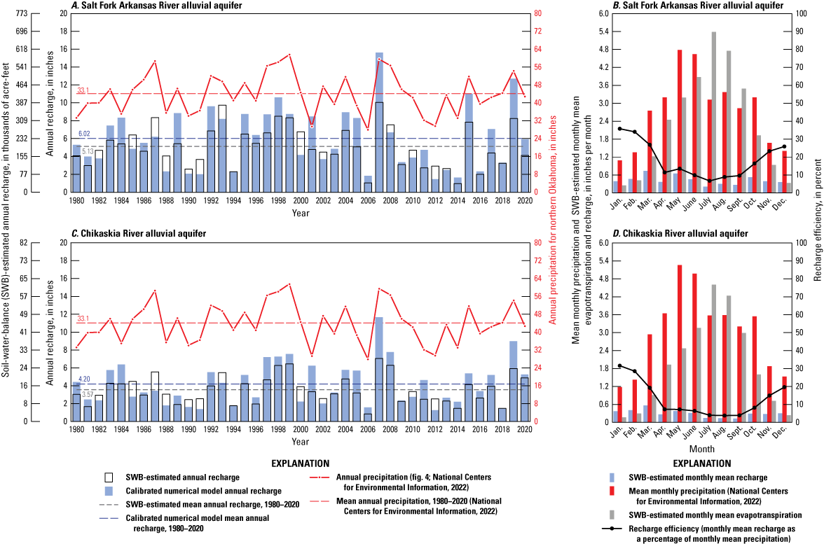
Precipitation and recharge of A, annual precipitation with annual recharge estimated by using the Soil-Water-Balance code (SWB; Westenbroek and others, 2010); B, monthly mean precipitation with mean monthly recharge and evapotranspiration estimated by using the SWB for the Salt Fork Arkansas River alluvial aquifer; C, annual precipitation with annual recharge estimated by using the SWB (Westenbroek and others, 2010); and D, mean monthly precipitation with mean monthly recharge and evapotranspiration estimated by using the SWB for the Chikaskia River alluvial aquifer, northern Oklahoma, 1980–2020.
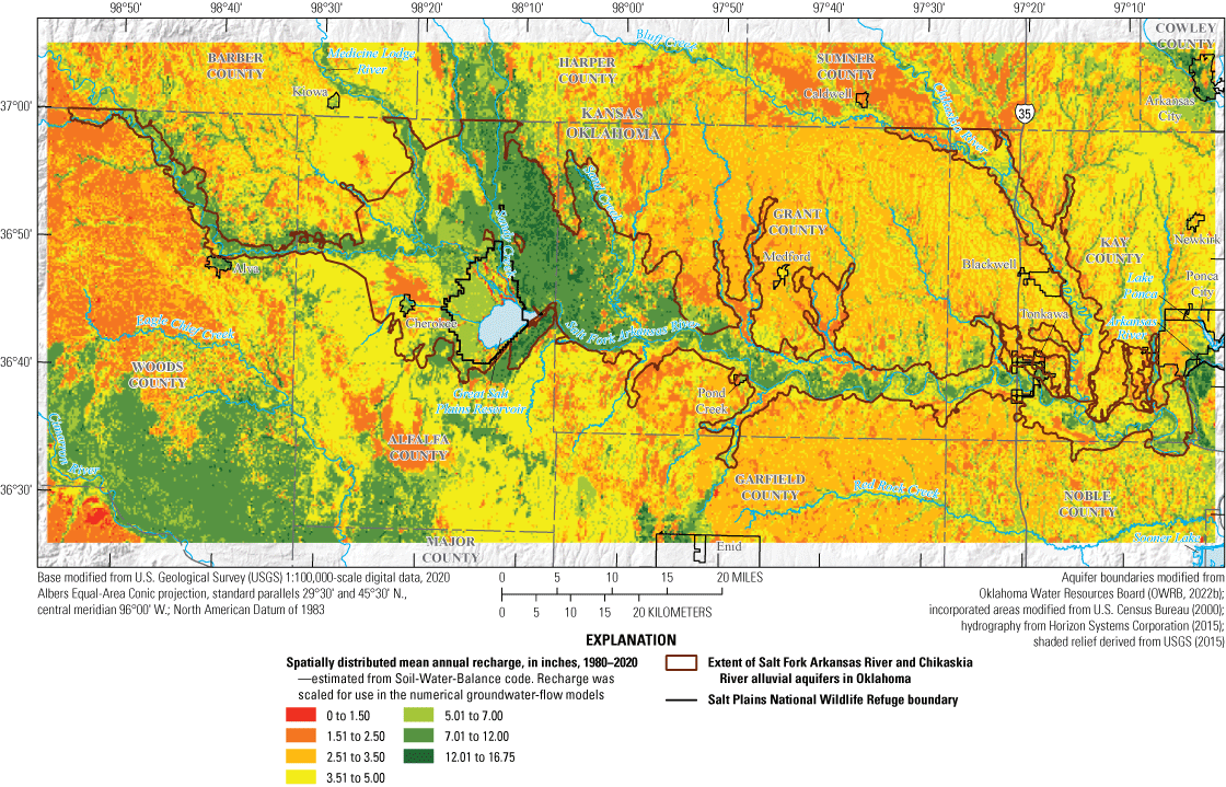
Mean annual recharge estimated by using the Soil-Water-Balance code (Westenbroek and others, 2010) in the Salt Fork Arkansas River and Chikaskia River alluvial aquifers, northern Oklahoma, 1980–2020.
Mean annual recharge rates estimated from SWB were compared to published estimates of mean annual recharge near the study area. Reed and others (1952) estimated a mean annual recharge rate of 4.2 in., or about 14.6 percent of the mean annual precipitation of 28.8 in. during a 1.5-year study period (July 1950–December 1951) in the Cimarron Terrace aquifer, which is mostly composed of dune sands in the southwest part of the study area (fig. 9). The authors cautioned that the recharge estimate may be biased low because the partial year 1950 was unusually dry. Belden (1997) estimated a mean annual recharge rate of 4.5 in. for the Chikaskia River alluvial aquifer, but that estimate was based largely on the estimate of Reed and others (1952). When calculated as a percentage of the mean annual precipitation for the study period 1980–2020, the mean annual recharge rate of 5.4 in. (16.3 percent of mean annual precipitation) that was estimated by using the WTF method for this study area is slightly higher than the published estimates of recharge for comparable aquifers in the study area.
The SWB code is a model used for simulation purposes, and SWB-estimated recharge must, therefore, be checked against and calibrated to field-based measurements or estimates of recharge such as those estimated using the WTF method. In other studies (Smith and others, 2017, 2021; Ellis, 2018; Ellis and others, 2020; Rogers and others, 2023), SWB-estimated recharge was calibrated by decreasing root-zone depths until the SWB-estimated mean annual recharge approximated the conceptual-model recharge. That method was also applied in this study, and the SWB-estimated recharge values reported above reflect those calibration methods. Additional fine-scale adjustment of SWB-estimated recharge was accomplished during calibration of the numerical model, as detailed in the “Numerical Groundwater-Flow Model” section of this report.
Saturated-Zone Evapotranspiration
Evapotranspiration is the process by which water is transferred to the atmosphere directly through evaporation and indirectly through plant transpiration. Most of this process either occurs at the land surface where precipitation pools as surface water or where it infiltrates the soil unsaturated zone and becomes available for uptake in the plant root zone (Lubczynski, 2009). These surface-water and unsaturated-zone components of evapotranspiration were not considered to be a part of the conceptual model for the Salt Fork Arkansas River and Chikaskia River alluvial aquifers, because they occur before infiltrating precipitation has reached the saturated zone to become groundwater recharge. An additional component of evapotranspiration, however, occurs in areas of the aquifer where the saturated zone intersects the plant root zone, most commonly in lower lying or wetland areas along streams (Lubczynski, 2009); this component of evapotranspiration (hereinafter referred to as “saturated-zone evapotranspiration”) was an important part of the conceptual-model water budget.
Rates of saturated-zone evapotranspiration are difficult to estimate over a large area such as the study area but were expected to be roughly proportional to (1) the area where the saturated zone intersects the plant root zone, (2) the mean depth to groundwater in that area during the growing season, and (3) the mean rate of transpiration associated with the assemblage of plants in that area. Based on groundwater-level observations (fig. 15), the area where the saturated zone intersects the plant root zone is small compared to the entire aquifer area and is mostly confined to the low-lying areas around the Great Salt Plains Reservoir and the stream corridors of the Salt Fork Arkansas River and its major tributaries. About 26,160 acres were classified as “freshwater emergent wetland,” “riverine,” “lake” (excepting the Great Salt Plains Reservoir), or “other” wetland (land area with frequently saturated or flooded soils [Cowardin and others, 1979]) by the National Wetlands Inventory (NWI; U.S. Fish and Wildlife Service, 2017). Open water, forested/shrubland, and wetland were excluded from that total because water levels in upland forested areas are far below the land surface and are mostly inaccessible to those plants. The saturated-zone component of evapotranspiration was assumed to be active during the April–October growing season (National Agricultural Statistics Service, 2020; Oklahoma Climatological Survey, 2015), greatest annually in wet and hot years, and greatest monthly in early summer (Scholl and others, 2005) when precipitation and temperature typically exceed their mean values for the year (fig. 5).
By using the assumptions just described pertaining to saturated-zone evapotranspiration, an attempt was made to estimate groundwater outflow by means of saturated-zone evapotranspiration estimated from daily water-level fluctuation data at wells with shallow depths to water according to the commonly used methods of White (1932). Wells with continuously measured groundwater-level data were not available during the study period in the study area, but streamgage-height data from the Alva, Blackwell, State Highway 11, and Tonkawa streamgages indicated daily declines in stream stage during daylight hours in summer low-flow conditions when there was minimal antecedent precipitation. These daily declines in stream stage, with rebounds at night, indicated that saturated-zone evapotranspiration was an active process in the Salt Fork Arkansas River and Chikaskia River alluvial aquifers, but the declines were too small to be accurately measured from the streamgage-height data. For this reason, the White (1932) methods were ultimately not used. Instead, an annual saturated-zone evapotranspiration rate of about 1.33 feet per year (Rogers and others, 2023) was assumed to be appropriate for the Salt Fork Arkansas River alluvial aquifer. If about 26,160 acres of wetland area had similar cover and depths to water, this assumed rate would correspond to an annual saturated-zone evapotranspiration outflow of 34,792 acre-ft/yr (15.1 percent of conceptual model outflows; table 10). This estimated annual saturated-zone evapotranspiration was allocated to areas of the Salt Fork Arkansas River alluvial aquifer upgradient and downgradient from the Great Salt Plains Reservoir and the Chikaskia River alluvial aquifer in proportion to wetland area (83.1, 15.1, and 1.8 percent, respectively). The area immediately upgradient from the Great Salt Plains Reservoir, especially to the north near Sandy Creek and the Salt Fork Arkansas River, is characterized by extensive wetland areas and flowing artesian wells. Groundwater-level altitudes in that area were expected to remain above the land surface and contribute to saturated-zone evapotranspiration continuously throughout the study period.
Streambed Seepage
Base flow can be measured directly in streams when the runoff component of streamflow is at or near zero (Garner and Bills, 2012). When base-flow measurements are made at multiple locations over a short period, they are commonly referred to as “synoptic base-flow” (seepage-run) measurements. These measurements can be used to calculate net streambed seepage and classify stream reaches as gaining or losing at a point in time. Gaining reaches exhibit an increase in base flow between the upstream and downstream endpoints of the reach, whereas losing reaches exhibit a decrease in base flow between the upstream and downstream endpoints. Streambed-seepage rates provided in this report were calculated as the difference in measured base flows (adjusted for tributary inflows) divided by the stream-reach length between measurement locations.
On March 2, 2020, synoptic base-flow measurements were collected by using the methods of Rantz and others (1982) during a period of minimal runoff and used in net streambed seepage computations. These synoptic base-flow measurements, along with streamflow data obtained from the active USGS streamgages listed in table 1 and a synoptic streamflow measurement made by the USGS at the OWRB White Eagle streamgage, served to delineate tributary inflow and base-flow conditions across the Salt Fork Arkansas River and Chikaskia River alluvial aquifers at a given point in time. These data, however, were not ideal for making conclusions about net streambed seepage, computed as the average of base-flow gains and losses over the study period. Excluding the Medicine Lodge and Chikaskia Rivers, tributaries contributed measured base flows ranging from 0.21 cubic feet per second (ft3/s) on an unnamed stream in Noble County to 95.3 ft3/s on Sandy Creek in Alfalfa County (fig. 21). Minor tributaries with unmeasured base flows were assumed to contribute no base flows and were not accounted for in computations of base flows in streams flowing across the Salt Fork Arkansas River and Chikaskia River alluvial aquifers. The base-flow measurements on the Salt Fork Arkansas River main stem generally increased downstream; the only exception was the reach immediately downstream from the Great Salt Plains Reservoir, which had a base-flow loss of 2.3 cubic feet per second per mile. The greatest base-flow gain (6.4 cubic feet per second per mile) occurred in the furthest downstream reach of the Salt Fork Arkansas River near Tonkawa, Okla.
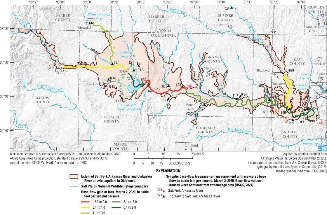
Synoptic streamflow (base-flow) measurements and estimated streambed seepage (base-flow gain or loss) in gaining and losing reaches of the Salt Fork Arkansas River and Chikaskia River alluvial aquifers, northern Oklahoma, March 2, 2020.
Net streambed-seepage terms for the conceptual model were assumed to be net outflows from the Salt Fork Arkansas River and Chikaskia River alluvial aquifers and were estimated primarily from mean annual base flows computed by using the BFI (Wahl and Wahl, 1995; Barlow and others, 2015) at selected streamgages in the study area. Because few streamgages had complete record during the 1980–2020 study period, the full period of record was used to compute mean annual base flows. Net streambed seepage in the reach upgradient from the Great Salt Plains Reservoir (70,571 acre-ft/yr, table 10) was roughly estimated as the mean annual base flow at USGS streamgage 07149520 Salt Fork Arkansas River at State Highway 11 near Cherokee, Okla. (hereinafter referred to as the “State Highway 11 streamgage”) multiplied by a drainage-area ratio of 1.3 (to account for ungaged drainage areas downstream) minus the mean annual base flows at the Kiowa streamgage and USGS streamgage 07148350 Salt Fork Arkansas River near Winchester, Okla. (hereinafter referred to as the “Winchester streamgage”) (fig. 1, table 4; tributary base flows are summarized in Smith and Gammill [2025]). Net streambed seepage in the reach downgradient from the Great Salt Plains Reservoir (89,774 acre-ft/yr, table 10) was estimated as the mean annual base flow at the Tonkawa streamgage multiplied by a drainage-area ratio of 1.1 (to account for ungaged drainage areas downstream) minus the mean annual base flow just downstream from the Great Salt Plains Reservoir (fig. 1, table 5) multiplied by 0.43 (the mean annual base-flow index for the period of record at the Jet streamgage). The tributary base flows are summarized in Smith and Gammill (2025), which were computed as the average of the mean annual base flow at the Jet streamgage and the mean annual reservoir releases (which include runoff and base-flow components; U.S. Army Corps of Engineers, 2023a). Net streambed seepage in the Chikaskia River reach (18,084 acre-ft/yr, table 10) was roughly estimated as the mean annual base flow at the Blackwell streamgage multiplied by a drainage-area ratio of 1.1 (to account for ungaged drainage areas downstream) minus the mean annual base flow at the Corbin streamgage multiplied by a drainage-area ratio of 1.4 (to account for ungaged drainage areas upstream) (fig. 1, table 4; tributary base flows are summarized in Smith and Gammill [2025]). The total net streambed seepage estimated for all reaches was 178,430 acre-ft/yr (table 10) and accounted for 77.3 percent of the total outflows in the conceptual-model water budget.
Well Withdrawals
Well withdrawals were assumed to equal the mean annual reported groundwater use for the period 1980–2020, or about 5,369 acre-ft for the Salt Fork Arkansas River and Chikaskia River alluvial aquifers combined (table 10). This mean annual reported groundwater use accounts for 2.3 percent of conceptual model outflows. Well withdrawals were greatest during dry and hot years because the most water was required during those years to grow healthy crops. Groundwater levels generally decrease during dry and hot years (especially during extended droughts) and increase during wet and cool years (fig. 18). The degree to which the groundwater levels fluctuate annually at a given location is related in part to the volume of nearby well withdrawals and the distribution (or concentration) of recharge near that location.
Change in Groundwater Storage
No wells with annual water-level measurements during the study period 1980–2020 were available for the Salt Fork Arkansas River and Chikaskia River alluvial aquifers, so estimating a net change in groundwater storage was not possible. The net change in groundwater storage in the Salt Fork Arkansas River and Chikaskia River alluvial aquifers was assumed to be a negligible component of the conceptual-model water budget. These assumptions were made with knowledge of net changes in groundwater storage calculated to be 5 percent or less of the water budget for other alluvial aquifers in Oklahoma, such as Salt Fork Red River and North Fork Red River (Smith and others, 2017, 2021)
Lateral Groundwater Flows
Net lateral groundwater flows of unknown magnitude and direction are exchanged between the Salt Fork Arkansas River and Chikaskia River alluvial aquifers and (1) adjacent alluvial deposits (for example, those in Kansas) and (2) adjacent and underlying bedrock units. Net lateral groundwater flows also occur between administrative sections (reaches) of the Salt Fork Arkansas River and Chikaskia River alluvial aquifers, but these components were not shown in the conceptual-model water-budget because lateral groundwater outflows to a reach are probably largely offset by lateral groundwater inflows to that reach (thus contributing minimal net lateral groundwater flows) (Gomo, 2011). No data were available to estimate net lateral groundwater flows, but they were expected to be a minor to negligible part of the conceptual-model water budget based on (1) the relatively small boundary between the alluvial aquifers and adjacent alluvial deposits and (2) the generally fine texture (and thus relatively low permeability) of bedrock units adjacent to and underlying the alluvial aquifers. Therefore, net lateral groundwater flows were calculated as the difference between the aquifer inflows (recharge) and summed aquifer outflows (saturated-zone evapotranspiration, streambed seepage, and well withdrawals) and were used to balance the conceptual-model water budget. The net lateral groundwater flows for the Salt Fork Arkansas River and Chikaskia River alluvial aquifers were outflows and together accounted for 2.8 percent of the conceptual-model water budget (table 10).
By comparison, net lateral groundwater flows accounted for 44 percent of the total inflows in the conceptual-model water budget for reach 1 of the Washita River alluvial aquifer (Ellis and others, 2020) and 65 percent of the total inflows in the conceptual-model water budget for the Canadian River alluvial aquifer (Ellis and others, 2017). Both of those alluvial aquifers, unlike the Salt Fork Arkansas River and Chikaskia River alluvial aquifers, were in contact with major bedrock aquifers. In the study area for this investigation, however, net lateral groundwater flows from the underlying bedrock units were expected to be small because those bedrock units (Hennessey and Sumner Groups) are composed primarily of shale and siltstone (figs. 9, 10), which typically do not transmit water at substantial rates. Studies of the salt flats east of the Great Salt Plains Reservoir serve as anecdotal evidence that some unquantified amount of saline groundwater is locally transmitted from the geologic units of the Hennessey Group to the Salt Fork Arkansas River alluvial aquifer. Johnson (2022) hypothesized that the saline groundwater east of the Great Salt Plains Reservoir is transmitted by lateral and vertical leakage through local collapse features overlying partially dissolved salt beds in the Hennessey Group. The lateral groundwater flows of the Salt Fork Arkansas River alluvial aquifer were assumed to be a negligible component of the conceptual-model water budget.
Conceptual-Model Water Budget
The conceptual-model water budget (table 10) summarizes mean water flows exchanged between each hydrologic boundary and the Salt Fork Arkansas River and Chikaskia River alluvial aquifers for the study period 1980–2020. The components of the water budget were estimated from analyses of available data or assumed on the basis of published analogs as described in the “Water-Budget Components” section of this report. Recharge accounts for 100.0 percent of the conceptual-model inflows to the Salt Fork Arkansas River and Chikaskia River alluvial aquifers, and net streambed seepage accounts for 77.3 percent of the outflows from the Salt Fork Arkansas River and Chikaskia River alluvial aquifers. Saturated-zone evapotranspiration (composing 15.1 percent of outflows) was the only other component estimated to be greater than 5 percent of inflows or outflows. Well withdrawals accounted for 2.3 percent of conceptual-model water-budget outflows, and net lateral groundwater flows accounted for 2.8 percent of conceptual-model water-budget inflows.
Numerical Groundwater-Flow Model
A finite-difference numerical model of the Salt Fork Arkansas River and Chikaskia River alluvial aquifers was constructed by using MODFLOW-2005 (Harbaugh, 2005) with the Newton formulation solver (MODFLOW-NWT, version 1.2.0; Niswonger and others, 2011) for improved solution of problems involving drying and rewetting. In the modular design of MODFLOW, each hydrologic boundary of the conceptual model, such as streambed seepage, recharge, or well withdrawals, is included as a boundary-condition package that, when activated, adds new inflow and outflow terms to the groundwater-flow equation being solved. Data inputs for each package are specified in human- and machine-readable text files. Model space is discretized into cells, and the cell size is the finest resolution at which spatially varying properties (such as land-surface altitude or horizontal hydraulic conductivity) may be represented and varied. Model time is discretized into time steps within stress periods. The stress-period length is the finest resolution at which temporally varying inflows and outflows may be represented and varied, and the time-step length is the finest length of time for which model outputs may be written. Selected numerical-model input values were adjusted to calibrate the model to available groundwater-level altitude and base-flow observations. The calibrated numerical groundwater-flow model inputs, outputs, metadata, directions for use, and ancillary data were published in Smith and Gammill (2025).
Spatial and Temporal Discretization
The model domain (fig. 22) of the Salt Fork Arkansas River and Chikaskia River alluvial aquifers was spatially discretized into 300 rows, 700 columns, 34,903 active cells (31,570 and 3,333 active cells for the Salt Fork Arkansas River and Chikaskia River alluvial aquifers, respectively) measuring 800 by 800 ft each, and a single convertible layer based on the hydrogeologic framework described in this report. Because the model consists of one layer, it was used to simulate only 2-dimensional (horizontal) flow between cells. The cell size was chosen to minimize model-processing time while still representing the variability of properties being simulated. The chosen cell size also ensured that the narrowest parts of the aquifers were represented by no fewer than three cells; model instability and groundwater-level volatility often occur in narrow parts of an aquifer area where groundwater flow is focused into fewer cells. The single convertible layer represented the undivided Quaternary age deposits with variable thickness determined from the hydrogeologic framework; the underlying bedrock was not represented as a layer. The altitude of the top of the aquifer, which was determined from a DEM, was multiplied by 1.01 in the numerical model to prevent confined aquifer conditions that occur as a side effect of model discretization when the simulated water-table altitude exceeds the altitude of the top of the aquifer. This multiplier, which adds about 10 ft to the altitude of the top of the aquifer, has no effect on most parts of the model where the simulated water-table altitude is below the altitude of the top of the aquifer. However, some simulated saturated-zone evapotranspiration and streambed seepage flows could be affected where the simulated water-table altitude is above the altitude of the top of the aquifer, which mostly occurs along simulated streams.
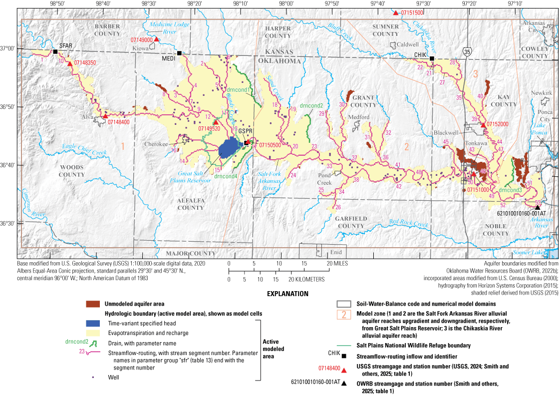
Model domain, active modeled area, hydrologic boundaries, and parameter zones for the numerical groundwater-flow model of the Salt Fork Arkansas River and Chikaskia River alluvial aquifers, northern Oklahoma.
The active modeled area (fig. 22) was initially derived from the extents (modified from OWRB [2022b]) as defined in the hydrogeologic framework of the Salt Fork Arkansas River and Chikaskia River alluvial aquifers. The active modeled area was expanded or contracted in some areas to remove isolated cells and ensure that each active cell was in connection with at least one other active cell. To improve model stability, the active modeled area was further modified by inactivating a relatively small number of model cells, mostly in thin, disconnected terrace lobes and in narrow areas along selected Salt Fork Arkansas River tributaries. These inactivated cells are shown as unmodeled aquifer area in figure 22.
The numerical model was temporally discretized into 492 monthly transient stress periods (each with two time steps to improve model stability) representing the 1980–2020 study period. The numerical-modeling period, hereinafter referred to as the “modeling period,” coincides with the 1980–2020 study period. An initial steady-state stress period represented mean annual inflows to, and outflows from, the aquifer. The steady-state solution was used as the initial condition for subsequent transient stress periods, as well as some groundwater-availability scenarios. The numerical model was constructed by using length and time units of feet and days, respectively.
Simulation of Hydrologic Boundaries and Hydraulic Properties
Hydrologic boundaries in the numerical model (fig. 22) define where and how water may enter or leave the model and include specified-flux and head-dependent boundaries (Harbaugh and others, 2000). Specified-flux boundaries were used to simulate recharge and well withdrawals. Head-dependent boundaries were used to simulate streambed seepage, spring seepage, and saturated-zone evapotranspiration. Lateral groundwater flows exchanged with surrounding and underlying bedrock units were not simulated because they were a small component of the conceptual model. Lateral groundwater flows between the Salt Fork Arkansas River and Chikaskia River alluvial aquifers were simulated in the numerical model, however. When available, hydrologic data, along with data-based assumptions and analogues, were used to estimate or constrain precalibration model inputs for each hydrologic boundary.
Recharge and Distribution With the Soil-Water-Balance Code
Recharge to the Salt Fork Arkansas River and Chikaskia River alluvial aquifers was simulated by using the Recharge package (Harbaugh and others, 2000). Recharge was spatially and temporally distributed for each month of the 1980–2020 study period by using outputs from the SWB method (Westenbroek and others, 2010). The SWB-output monthly recharge grids were converted to model units of feet per day and used as precalibration numerical-model inputs. These inputs were then scaled with multipliers during the numerical-model calibration (described in the “Calibration” section) to improve agreement between the simulated recharge rate and the conceptual-model recharge determined by the WTF method. The initial steady-state recharge-rate multiplier (rch001, table 13) of 1.0 was allowed to vary within 20.0 percent (between 0.8 and 1.2); the initial transient recharge-rate multipliers (rch002–rch493, table 13) of 1.0 for each month within the period 1980–2020 were allowed to vary between 0.50 and 2.00 (Smith and Gammill, 2025). A narrower range was required for the steady-state recharge-rate multiplier to keep the numerical-model recharge closely aligned with the conceptual-model recharge.
Table 13.
Calibration parameters for the numerical groundwater-flow model of the Salt Fork Arkansas River and Chikaskia River alluvial aquifers, northern Oklahoma, 1980–2020.[A more detailed version of this table is available in the associated data release (Smith and Gammill, 2025). drn, MODFLOW Drain package simulating spring seepage; evt, MODFLOW Evapotranspiration package simulating saturated-zone evapotranspiration; hyd, horizontal hydraulic conductivity; rch, MODFLOW Recharge package simulating recharge; sfr, MODFLOW Streamflow-Routing package, version 2, simulating streambed seepage; sto, storage properties]
Lateral Groundwater Flows
Lateral groundwater flows were not simulated in the numerical model because of (1) the fine-grained nature (relative impermeability) of the bedrock geologic units underlying the Salt Fork Arkansas River and Chikaskia River alluvial aquifers; (2) the narrow alluvium (relatively minimal cross sectional area and presumed groundwater flow) of the Salt Fork Arkansas, Chikaskia, and Medicine Lodge Rivers along the Kansas State line; (3) the narrow alluvium (relatively minimal cross sectional area and presumed groundwater flow) of the Salt Fork Arkansas River at the downgradient end of the Salt Fork Arkansas River alluvial aquifer; and (4) the relatively low rate of lateral groundwater flow in the conceptual-model water budget (table 10). Lateral groundwater flows between the alluvial aquifers and underlying bedrock units, which are often simulated by using general-head boundaries (GHBs), were not simulated because of (1) the minimal contributions of these flows the conceptual-model water budget and (2) the increased complexity associated with these boundaries during numerical model calibration and in groundwater-availability scenarios.
Streams
Named streams listed in the National Hydrography Dataset Plus (Horizon Systems Corporation, 2015) were simulated by using the Streamflow-Routing package, version 2 (SFR2) (Niswonger and Prudic, 2005); small, unnamed streams were not simulated. Only base flow (no runoff) was simulated in the SFR2 streams. Inflows for SFR2 stream cells included base flows routed from upstream segments, specified inflows (base flows) from unsimulated tributary streams, and streambed seepage from the aquifer; outflows for SFR2 stream cells included base flows routed downstream and streambed seepage to the aquifer. SFR2 computes streambed seepage between the aquifer and stream according to Darcy’s Law (Darcy, 1856; Bennett, 1976); the flow exchanged between the aquifer and stream is the product of the streambed conductance and the difference between the water-table altitude and stream stage, where the streambed conductance is the product of the hydraulic conductivity of the streambed sediments and the area of the stream channel divided by the streambed thickness. In SFR2, simulated base flows are calculated in each model cell and are routed downstream by segments (groups of cells with uniform hydraulic properties). Accumulated base flows are passed to the next downstream segment until flows are routed out of the active modeled area.
All SFR2 stream segments (1–53, fig. 22) were initially assigned a streambed thickness (sbb01–sbb53, table 13) of 2.0 ft and a streambed hydraulic conductivity (sbk01–sbk53, table 13) of 7.0 ft/d (based on Rogers and others [2023] and Smith and others [2021], respectively), but these properties were adjusted during calibration to be within ranges of 1.0–5.0 ft and 2.0–12.0 ft/d, respectively (Smith and Gammill, 2025). The streambed widths of stream segments (sbw01–sbw53, table 13) were estimated from aerial photographs (Microsoft Corporation, 2022) and ranged from 10 to 320 ft (Smith and Gammill, 2025), gradually increasing downstream. The channel widths of some streams were increased to as much as double the estimated values during calibration; increased stream widths resulted in decreased simulated stream stages and corresponding increases in the flow from the aquifer to the stream, allowing parts of the model to drain more efficiently. The streambed depth below land surface (sbd01–sbd53, table 13) was initially set to 10.0 ft and was adjusted during calibration to be within the range of 0.0–13.0 ft for the Salt Fork Arkansas River downgradient from the Great Salt Plains Reservoir, 0.0–12.0 ft for the Chikaskia River, and 0.0–11.0 ft for other simulated streams (Smith and Gammill, 2025). At model run time, the streambed depth was subtracted from the land-surface altitude, as represented by a 10-m-resolution DEM (USGS, 2015). This streambed incision is necessary to compensate for lost spatial resolution of the stream channel (altitude averaging) caused by the large DEM cell size. When land-surface altitudes of actual features are represented by a DEM cell, the lowest altitudes (often stream channels) and highest altitudes (summits) are generalized to a single value—the mean land-surface altitude in the cell. The difference between the actual altitude of those features and the cell-averaged altitude depends on the local altitude relief and the cell size.
Streamgage records were used to estimate base-flow inflows where available (tables 4, 5). However, streamgages are not always located where, or active when, the data are needed, and streamgage data must be systematically adjusted or synthesized to approximate the needed data. Monthly base-flow inflows were estimated for the Salt Fork Arkansas River, Medicine Lodge River, and Chikaskia River at the boundary of the active modeled area primarily by using streamgage records from the Winchester streamgage, Kiowa streamgage, and Corbin streamgage, respectively; these inflows are denoted on figure 22 as “SFAR,” “MEDI,” and “CHIK.” In the case of Salt Fork Arkansas River inflows, missing records from the Winchester streamgage (October 1993–December 2020) were synthesized from records at the Alva streamgage downstream by using a reduction factor of 0.7; this factor was determined from the mean ratio of monthly base flows for the period when records were available at both streamgages. CHIK inflows were determined as the monthly base flows at the Corbin streamgage, multiplied by a factor of 1.4 to account for ungaged areas mostly along the Bluff Creek tributary to the Chikaskia River (fig. 22). Monthly base-flow inflows also were specified at the outlet of Great Salt Plains Reservoir by using available record (1980–92) at the Jet streamgage or monthly U.S. Army Corps of Engineers (2023b) reservoir releases (1995–2020); these inflows are denoted on figure 22 as “GSPR.” Large flood-control reservoirs like the Great Salt Plains Reservoir complicate the simulation of streambed seepage in numerical groundwater-flow models because they are designed to impound runoff and gradually release it downstream. An unknown portion of those releases is interpreted as base flows by base-flow-separation algorithms used on streamgage records downstream. Releases from the Great Salt Plains Reservoir were multiplied by 0.43, which was the mean base-flow-index value computed for the available record at the Jet streamgage during the study period. The releases were reduced in an attempt to simulate only true base flows, derived directly from groundwater discharge, in simulated streams. These reduced releases were used as Great Salt Plains Reservoir specified inflows. Tributaries with no specified inflows were assumed to contribute negligible base flows to simulated streams.
Permitted surface-water withdrawals, which have been simulated in other alluvial aquifer models (for example, Smith and others, 2021, and Rogers and others, 2023), were not simulated in the numerical model of the Salt Fork Arkansas River and Chikaskia River alluvial aquifers. Surface-water withdrawals, predominantly for irrigation use, were expected to be disproportionately derived during times of high runoff because of the relatively high salinity of surface water (fig. 12) during base-flow conditions. In 2020, active surface-water permits on the Salt Fork Arkansas River and tributaries in Oklahoma excluding the Chikaskia River totaled 6,058.3 acre-ft/yr (OWRB, 2022d); of that total, active permits upgradient from the Great Salt Plains Reservoir accounted for 3,993.0 acre-ft/yr and were all located along Sandy Creek. In 2020, active permits on the Chikaskia River and tributaries in Oklahoma totaled 12,668.8 acre-ft/yr (OWRB, 2022d).
Lake
The Great Salt Plains Reservoir, which is the only large lake overlying the Salt Fork Arkansas River and Chikaskia River alluvial aquifers, was simulated by using the Time-Variant Specified-Head boundary package (Harbaugh and others, 2000). Monthly lake altitude data (USACE, 2023b) were available for November 1994 through the end of the modeling period (December 2020) and were assigned as starting and ending heads for the corresponding stress periods of the transient simulation. Starting and ending heads for the preceding transient stress periods and the steady-state stress period were assigned the normal pool altitude of 1,125.3 ft above NAVD 88. This value was converted from 1,125.0 ft above the National Geodetic Vertical Datum of 1929 (NGVD 29; USACE, 2023b) using VERTCON (National Oceanic and Atmospheric Administration, 2023).
Springs and Seeps
Some groundwater was expected to flow out of the Salt Fork Arkansas River alluvial aquifer through distributed spring and seep discharge areas where terrace deposits extend across major groundwater divides. Spring and seep discharge was simulated along the eastern edge of four selected terrace lobes (drncond1–4; fig. 22) by using the Drain package (Harbaugh and others, 2000). The simulated drains were necessary to prevent these areas from pooling groundwater, but the presence of small spring or distributed seep discharges is indicated by an increased density of vegetation and ponds corresponding to the simulated drain areas. The flow from the aquifer at a drain cell is the product of the specified drain conductance and the difference between the simulated water-table altitude and the specified drain altitude; however, there is no drain flow into the aquifer when the simulated water-table altitude is less than the specified drain altitude. Flows to drains are routed out of the active modeled area. The initial drain conductance varied by location but was roughly equivalent to the horizontal hydraulic conductivity of the aquifer multiplied by the length of one numerical-model cell (about 10,000 square feet per day [ft2/d]). During calibration, drain conductance values were grouped, and each group was allowed to vary between 1,000 and 100,000 ft2/d. The drain altitude was assigned as the DEM altitude minus 5–7 ft to account for lost spatial resolution resulting from the relatively large DEM cell size of 10 m.
Saturated-Zone Evapotranspiration
Saturated-zone evapotranspiration was simulated by using the Evapotranspiration package (Harbaugh and others, 2000) and was expected to occur near streams and riparian wooded areas along the Salt Fork Arkansas River and perennial tributaries. Maximum rates of saturated-zone evapotranspiration were assumed to not exceed the difference between potential and actual evapotranspiration as computed by using the SWB method; this assumption prevented the summed components of evapotranspiration from exceeding the potential evapotranspiration. Arrays representing the potential minus actual evapotranspiration for each monthly transient stress period (evtjan–evtdec, table 13) and the steady-state stress period (evtavg, table 13) were initially scaled by a factor of 1.0. During calibration, the scaling factors were allowed to vary independently in the range of 0.5–1.5 (Smith and Gammill, 2025). The evapotranspiration extinction (root-zone) depth (evtextd, table 13), or the depth below land surface at which the saturated zone becomes inaccessible to plants, was initially set at 1.0 ft in the active modeled area, which was consistent with the mean plant root-zone depth specified for grass/pasture and cropland (the dominant land-cover types, fig. 3) in the SWB code. During calibration, the evapotranspiration extinction depth was allowed to vary in the range of 0.8–1.2 ft. The saturated-zone evapotranspiration reference altitude (evttop, table 13) was initially set to the land-surface altitude of each cell but was adjusted during calibration by a multiplier that was allowed to vary within the range of 1.001–1.015. The narrow range used for the reference altitude multiplier was necessary for numerical model stability (Rogers and others, 2023).
Well Withdrawals
Well withdrawals for the 1980–2020 study period were simulated by using the Well package (Harbaugh and others, 2000). Annual reported groundwater use for each permit was evenly distributed among all well locations recorded for that permit (OWRB, 2022d). In the case of permits for which there were no recorded wells, a single well was placed in the center of the land parcel recorded for the permit. Annual reported groundwater use was temporally split into model stress periods by using the mean monthly water demand distribution (fig. 23; OWRB, 2012a) from Oklahoma Comprehensive Water Plan water-management planning basins 67–70 (fig. 2; OWRB, 2022c). The monthly water demand for irrigation was greatest in the summer months; July–September accounted for about 91 percent of irrigation groundwater use (fig. 23). The monthly water demand for public supply also was greatest in the summer months; however, July–September only accounted for about 34 percent of public-supply groundwater use (fig. 23). The Well package file contains some withdrawals for wells outside of the active modeled area. These withdrawals were not simulated in the model but were included in the Well package file in case the active modeled area is expanded in future versions of the model.
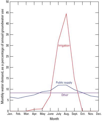
Monthly water demand by groundwater-use type for Oklahoma Comprehensive Water Plan water-management planning basins 67–70, averaged, Salt Fork Arkansas River and Chikaskia River alluvial aquifers, northern Oklahoma (fig. 2; Oklahoma Water Resources Board [OWRB], 2022c). Data from OWRB (2012a).
Storage and Hydraulic Properties
The Upstream Weighting package of MODFLOW-2005 (Niswonger and others, 2011) was used to represent storage and hydraulic properties of the Salt Fork Arkansas River alluvial aquifer. Initial storage and hydraulic property values were assumed to be similar to those used in numerical models for other alluvial aquifers in Oklahoma (Ellis and others, 2017, 2020; Smith and others, 2017, 2021; Rogers and others, 2023). The storage and hydraulic property values were adjusted during model calibration but were held spatially uniform and temporally constant through all stress periods in all simulations. The specific yield (sy1, sy2, and sy3, table 13) for the Salt Fork Arkansas River and Chikaskia River alluvial aquifers was initially set to 0.065 (dimensionless) and was allowed to vary in the range of 0.02–0.10, based on values from aquifer tests in the nearby Cimarron Terrace aquifer (Reed and others, 1952). The specific storage (ss, table 13) was initially set to 1×10⁻⁴ ft–1 based on Fetter and Kreamer (2021) and was allowed to vary plus or minus one order of magnitude (from 1×10⁻³ to 1×10⁻⁵ ft–1). Horizontal hydraulic conductivity (hkpp001–hkpp788, table 13) was represented with 788 pilot points (1–788, fig. 24; Doherty, 2010) placed at 8,000-ft intervals (one at every 10th column and row) within an 11,400-ft buffer (the approximate diagonal distance between pilot points) of the aquifer boundary. Pilot points are regularly spaced control points used to support an interpolation of cell-based horizontal hydraulic conductivity values across an active modeled area. The 788 pilot points were assigned an initial horizontal hydraulic conductivity value of 32.1 ft/d and were allowed to vary independently between 10 and 150 ft/d (Smith and Gammill, 2025) during calibration; the lower bound was from Rogers and others (2023), but the upper bound was adjusted upward from a value of 100 ft/d in Rogers and others (2023) because of improved calibration outcomes. Areas between pilot points were interpolated by kriging the pilot-point values before each model run to create the horizontal hydraulic conductivity array read by the numerical model (Doherty, 2010). Pilot-point kriging factors are outlined in model input files and model-preprocessing scripts in Smith and Gammill (2025).
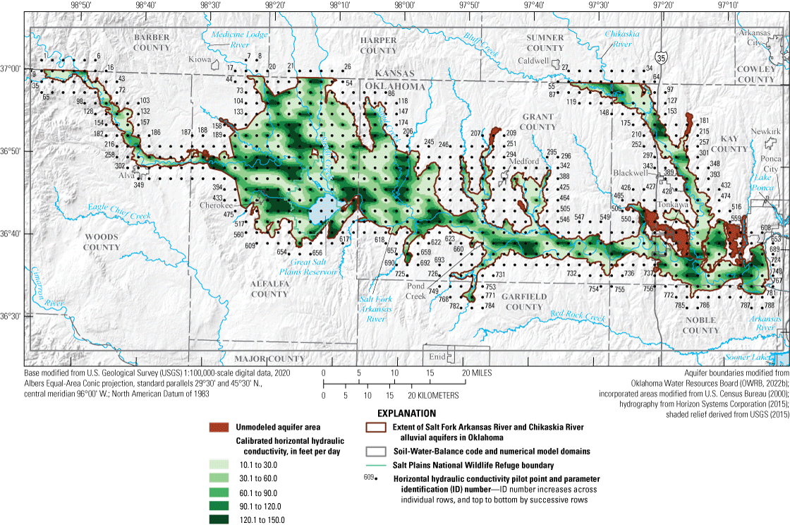
Horizontal hydraulic conductivity pilot points and calibrated horizontal hydraulic conductivity for the numerical groundwater-flow model of the Salt Fork Arkansas River and Chikaskia River alluvial aquifers, northern Oklahoma.
Solver Settings and Budget Percentage Discrepancies
Most of the settings for the Newton solver were unchanged from suggested input values (Winston, 2018), which were converted to model units of feet and days. The head tolerance was increased to 0.075 ft, and the flux tolerance was increased to 5,000 cubic feet per day. These settings improved model stability while keeping solution budget percentage discrepancies under 1.0 percent for all 493 stress periods; the largest budget percentage discrepancy (by absolute value) was 0.49 percent in stress period 382 (Smith and Gammill, 2025).
Calibration
Model calibration is the process of systematically changing selected model input values (parameters) within predetermined limits to improve the fit between model-simulated data and observed data (calibration targets). The preferred calibration results (1) minimize the differences (residuals) between simulated and observed data and (2) conform to the predetermined conceptual model. The calibration process for the numerical model included both manual and automated adjustments of parameters. The manual calibration approach primarily focused on aligning the numerical-model water budget (particularly the recharge and streambed seepage components) to the conceptual-model water budget. The manual calibration also involved selected structural elements of the model, such as boundary altitudes, that are not easily adjusted by automated calibration methods. The automated calibration approach focused solely on minimizing residuals and used the PEST++ iterative ensemble smoother (White, 2018) to reduce run times associated with the calibration of highly parameterized models.
Calibration Targets
The suite of calibrated parameter values was evaluated based on the minimization of an objective function. The objective function was calculated as the sum of squared weighted residuals for calibration targets in seven observation groups: water-table-altitude observations, base-flow observations at the Alva streamgage, base-flow observations at the State Highway 11 streamgage, base-flow observations at the Tonkawa streamgage, base-flow observations at the Blackwell streamgage, base-flow observations (estimated) at the OWRB White Eagle streamgage, and selected conceptual-model (recharge and streambed-seepage) flows (tables 14, 15). The streamgages used for base-flow calibration had observations (or synthesized observations) during the study period and were not used to define base-flow inflows to the active modeled area (fig. 25).
Table 14.
Components of the objective function for the automated precalibration of the numerical groundwater-flow model of the Salt Fork Arkansas River and Chikaskia River alluvial aquifers, 1980–2020.[The objective function is calculated as the sum of squared weighted residuals. Table 1 provides the full station names for streamgages listed in the source column. NAVD 88, North American Vertical Datum of 1988; SS, steady-state simulation; TR, transient simulation; min, minimum; max, maximum; RMSE, root-mean-square error; OWRB, Oklahoma Water Resources Board; USGS, U.S. Geological Survey; E, base-10 exponent (for example, 1.7E-07 equals 1.7×10⁻⁷); ft, foot; ft3/s, cubic foot per second; acre-ft/yr, acre foot per year]
| Observation group | Source | Number of observations | Observation weight | Precalibration residuals (feet unless specified otherwise) | ||||||||
|---|---|---|---|---|---|---|---|---|---|---|---|---|
| SS | TR | SS | TR | Min | Mean | Max | Inter-quartile range | RMSE | Objective function component | |||
| (square feet) | (percent) | |||||||||||
| Groundwater-level altitude (feet above NAVD 88) (headobs) | Water-table-altitude observations (OWRB, 2022a; USGS, 2024) | 68 | 1,261 | 7.30E−01 | 7.30E−01 | −35 | −2.9 | 36.6 | 9.7 | 7.1 | 66,695 | 33.7 |
| Base flow, ft3/s (gageobs1) | Alva streamgage (07148400; USGS, 2024) | 1 | 165 | 3.40E−05 | 1.70E−07 | −48.2 | 1.8 | 66.4 | 11.5 | 0.3 | 38 | 0 |
| Base flow, ft3/s (gageobs2) | State Highway 11 streamgage (07149520; USGS, 2024) | 1 | 86 | 2.00E−05 | 1.00E−07 | −666.7 | −139.4 | 163.3 | 161.1 | 1.1 | 616 | 0.3 |
| Base flow, ft3/s (gageobs3) | Tonkawa streamgage (07151000; USGS, 2024) | 1 | 492 | 4.00E−05 | 2.00E−08 | −1,678.70 | 73.6 | 4,318.60 | 163.3 | 11.4 | 64,370 | 32.5 |
| Base flow, ft3/s (gageobs4) | Blackwell streamgage (07152000; USGS, 2024) | 1 | 483 | 2.00E−05 | 1.00E−08 | −314.4 | 45.5 | 1,008.30 | 71.9 | 3.8 | 7,274 | 3.7 |
| Base flow, ft3/s (gageobs5) | OWRB White Eagle Streamgage (621010010160-001AT; estimated as sum of the base flows at the Tonkawa and Blackwell streamgages plus 10 percent) | 1 | 483 | 1.00E−05 | 5.00E−09 | −1,515.70 | 150.5 | 6,123.80 | 272.9 | 6.2 | 18,998 | 9.6 |
| Conceptual model (recharge and stream-seepage) flows, acre-ft/yr (budgetobs) | Conceptual model (table 10) | 5 | 5 | 3.00E−03 | 3.00E−03 | −31,398.60 | −3,059.70 | 20,571.80 | 36,679.50 | 63.3 | 40,115.80 | 20.2 |
| Total | -- | 78 | 2,975 | -- | -- | -- | -- | -- | -- | -- | -- | -- |
| Objective function | -- | -- | -- | -- | -- | -- | -- | -- | -- | -- | 198,108 | -- |
Table 15.
Components of the objective function for the automated precalibration of the numerical groundwater-flow model of the Salt Fork Arkansas River and Chikaskia River alluvial aquifers, 1980–2020.[The objective function is calculated as the sum of squared weighted residuals. Table 1 provides the full station names for streamgages listed in the source column. NAVD 88, North American Vertical Datum of 1988; SS, steady-state simulation; TR, transient simulation; min, minimum; max, maximum; RMSE, root-mean-square error; OWRB, Oklahoma Water Resources Board; USGS, U.S. Geological Survey; E, base-10 exponent (for example, 1.7E-07 equals 1.7×10⁻⁷); ft, foot; ft3/s, cubic foot per second; acre-ft/yr, acre foot per year]
| Observation group | Source | Number of observations | Observation weight | Calibrated residuals | ||||||
|---|---|---|---|---|---|---|---|---|---|---|
| (feet unless specified otherwise) | ||||||||||
| SS | TR | SS | TR | Min | Mean | Max | Inter-quartile range | RMSE | ||
| Groundwater-level altitude (feet above NAVD 88) (headobs) | Water-table-altitude observations (OWRB, 2022a; USGS, 2024) | 68 | 1,261 | 7.30E−01 | 7.30E−01 | −28.7 | −3 | 30 | 7.3 | 5.7 |
| Base flow, ft3/s (gageobs1) | Alva streamgage (07148400; USGS, 2024) | 1 | 165 | 3.40E−05 | 1.70E−07 | −57.1 | 0.6 | 64.2 | 11.6 | 0.1 |
| Base flow, ft3/s (gageobs2) | State Highway 11 streamgage (07149520; USGS, 2024) | 1 | 86 | 2.00E−05 | 1.00E−07 | −678.7 | −150.9 | 122.3 | 163.5 | 2.1 |
| Base flow, ft3/s (gageobs3) | Tonkawa streamgage (07151000; USGS, 2024) | 1 | 492 | 4.00E−05 | 2.00E−08 | −1,713.30 | 39.4 | 4,258.10 | 153.5 | 5.6 |
| Base flow, ft3/s (gageobs4) | Blackwell streamgage (07152000; USGS, 2024) | 1 | 483 | 2.00E−05 | 1.00E−08 | −311.6 | 42.4 | 1,006.30 | 70.6 | 3.6 |
| Base flow, ft3/s (gageobs5) | OWRB White Eagle streamgage (621010010160-001AT; estimated as sum of Tonkawa and Blackwell streamgages plus 10 percent) | 1 | 483 | 1.00E−05 | 5.00E−09 | −1,547.00 | 108.1 | 6,052.60 | 264.5 | 4.4 |
| Conceptual model (recharge and stream-seepage) flows, acre-ft/yr (budgetobs) | Conceptual model (table 10) | 5 | 5 | 3.00E−03 | 3.00E−03 | −10,188.70 | −1,357.50 | 7,102.80 | 8,669.10 | 17.4 |
| Total | -- | 78 | 2,975 | -- | -- | -- | -- | -- | -- | -- |
| Objective function | -- | -- | -- | -- | -- | -- | -- | -- | -- | -- |
Base-flow observation groups accounted for nearly half (46.1 percent) of the precalibration objective function; the precalibration weighting scheme reflects an assumption that base-flow observations are more important than groundwater-level altitude observations for the purpose of determining the parameter values that are most influential in estimating water availability (the primary subject of this report). Base flows are generally more sensitive to changes in specific yield, which is a primary factor determining the volume of water in the aquifer, whereas groundwater-level altitudes are generally more sensitive to changes in horizontal hydraulic conductivity, which is a primary factor determining the rates of groundwater flow in the aquifer (Arnold and others, 2000). Also, because streamgages monitor base flows originating from all areas upstream, these base-flow observations are more likely to summarize regional (rather than localized) conditions in the aquifer than local well observations.
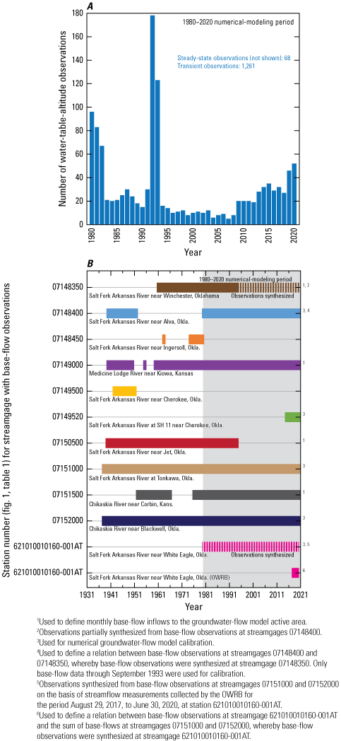
The temporal distribution of U.S. Geological Survey and Oklahoma Water Resources Board (OWRB) A, groundwater-level-altitude observations; and B, streamflow observations used for calibration of the numerical groundwater-flow model of the Salt Fork Arkansas River and Chikaskia River alluvial aquifers, northern Oklahoma.
Groundwater-Level Altitude Observations
The Head Observation (HOB) package (Hill and others, 2000) was used to compare simulated groundwater-level altitudes to observed groundwater-level altitudes in the Salt Fork Arkansas River and Chikaskia River alluvial aquifers for the modeling period 1980–2020. Observed groundwater-level altitudes were calculated by subtracting the depth-to-water measurements from the land-surface altitude obtained from a 10-m DEM (USGS, 2015). For consistency, the land-surface altitude was obtained from the DEM, even when the data source provided a land-surface altitude. Groundwater-level altitude observations were filtered such that only one observation per cell per stress period was included in the HOB package. Only 1,261 groundwater-level-altitude observations (OWRB, 2022a; USGS, 2024) from 68 wells were included for the transient simulation in the HOB package (fig. 25A, tables 14, 15). Groundwater-level-altitude observations from the transient simulation were averaged by well to derive 68 calibration targets (one for each well) for the steady-state simulation because few groundwater-level-altitude observations were available at the beginning of the modeling period (1980; fig. 25A, tables 14, 15).
Base-Flow Observations
Base-flow observations were available for 492 months (the full modeling period) at the Tonkawa streamgage on the Salt Fork Arkansas River (07151000, fig. 25B), 86 months at the State Highway 11 streamgage on the Salt Fork Arkansas River (07149500), and 483 months at the Blackwell streamgage on the Chikaskia River (07152000). Base-flow observations were available for 491 months at the Alva streamgage on the Salt Fork Arkansas River (07148400), but only the first 165 months (through September 1993) at the Alva streamgage were used as calibration targets because the rest were used to formulate Salt Fork Arkansas River inflows. Base-flow records also were available for the 2017–20 period at the OWRB White Eagle streamgage near the downgradient end of the active modeled area (fig. 2; streamgage data available in Smith and Gammill [2025]). Base-flow records at the OWRB White Eagle streamgage were used to calculate a scaling factor of 1.1 by which monthly base flows for 483 months could be estimated from summed base-flow observations at the Tonkawa streamgage on the Salt Fork Arkansas River and the Blackwell streamgage on the Chikaskia River (fig. 25). The monthly mean base flows determined for five streamgages (the Alva, State Highway 11, Tonkawa, and OWRB White Eagle streamgages on the Arkansas River, and the Blackwell streamgage on the Chikaskia River) (tables 14, 15) were used as calibration targets for the transient simulation. The mean annual base flows for these five streamgages were also used as calibration targets for the steady-state simulation. Base-flow observations from other selected streamgages were not used as calibration targets because they (1) were previously used to define inflows for SFR2 or (2) had periods of record that were less than 10 years, and thus too short to be representative of streamflow conditions during the modeling period.
Conceptual-Model Flow Observations
Conceptual-model flow observations consisted of five steady-state observations and five transient observations (tables 14, 15) derived from the conceptual-model water budget (table 10); both sets of observations were identical and were compared to the respective steady-state and transient budgets. Each set of observations included three recharge observations, one for each subarea, and two streambed seepage observations, upgradient and downgradient from the Great Salt Plains Reservoir dam. These conceptual model recharge and streambed seepage flows were initially used as observations to ensure that the numerical model budget honored the conceptual model. During manual calibration of the numerical model, however, the simulated base flows at the streamgages furthest downstream were always underestimated compared to the base-flow observations. During automated calibration, the conceptual-model recharge and streambed-seepage flow observations were increased by about 10 percent to increase simulated base flows and improve the calibration outcomes.
Calibration Results
Calibration results were evaluated based on the reduction of the objective function and the general fit of the calibrated numerical-model water budget to the predetermined (adjusted) conceptual-model water budget. Automated calibration reduced the objective function total by about 60 percent from precalibration inputs (tables 14, 15). Most of that reduction resulted from reducing conceptual-model-flow residuals from 20.2 to 3.8 percent of the objective function and base-flow residuals at the Tonkawa streamgage from 32.5 to 19.2 percent of the objective function. Some observation groups, most notably groundwater-level-altitude observations, increased in the percent contribution to the objective function after calibration. However, the objective function component decreased for all observation groups except for base-flow observations at the State Highway 11 streamgage (gageobs2).
Observation-Sensitivity Analysis
As part of the calibration process, an observation-sensitivity analysis was performed with the iterative parameter estimation software package PEST (Doherty, 2010) to identify which parameters were most effective, and most ineffective, at reducing the objective function. PEST measures the changes in calibration-target residuals resulting from 1-percent changes in each parameter and records those changes in a Jacobian matrix with dimensions equal to the number of observations by the number of parameters (Doherty, 2010). Parameters with the greatest effects on calibration-target residuals have the greatest observation sensitivities. Observation sensitivity values and ranks for individual parameters are available in the companion USGS model archive data release (Smith and Gammill, 2025) that accompanies this report.
Parameters closely linked, either spatially or temporally, to observations typically had the greatest observation sensitivities in the numerical model. Parameters with the greatest observation sensitivities were the saturated-zone evapotranspiration reference altitude multiplier (evttop) and extinction depth (evtextd), the steady-state recharge-rate multiplier (rch001), the steady-state saturated-zone evapotranspiration-rate multiplier (evtavg), and the streambed depth for SFR2 zone 10 (sbd10) (Smith and Gammill, 2025; table 13). Horizontal hydraulic conductivity pilot points 145, 203, 204, 218, and 282 (hkpp145, hkpp203, hkpp204, hkpp218, and hkpp282) were the only horizontal hydraulic conductivity pilot points with sensitivities ranking in the top 20 of the 1,516 calibration parameters. The horizontal hydraulic conductivity pilot points with the highest-ranking sensitivities were in parts of the aquifer with high spatial and temporal density of groundwater-level-altitude observations. The specific yield for reach 1 (sy1) and the specific yield for reach 2 (sy2) ranked 8 and 14, respectively, of the 1,516 calibration parameters. The steady-state recharge-rate multiplier parameter (rch001) determined how much recharge was applied in the steady-state simulation, which included many of the groundwater-level altitude observations (Smith and Gammill, 2025). The specific yield parameters sy1 and sy2 controlled the volume of water released from storage as streambed seepage to streams across the entire aquifer, which in turn partially controlled how much base flow was simulated in the Salt Fork Arkansas River.
To simplify and graphically summarize the observation-sensitivity analysis, parameters were placed into six groups (table 13), and observation-group sensitivities were calculated as the sum of the Jacobian matrix output for each parameter group (fig. 26). Sensitivities less than 1×10⁻⁵ with respect to the drain parameter group indicate no sensitivity to those parameters. All observation groups were most sensitive to changes in saturated-zone-evapotranspiration (evt) parameters. Base-flow observations also were sensitive to changes in recharge (rch) parameters, and to a lesser degree, hydraulic conductivity (hyd) and streamflow-routing (sfr) parameters; groundwater-level-altitude and conceptual-model flow observations were roughly equally sensitive to recharge (rch) and hydraulic conductivity (hyd) parameters. The storage (sto) parameter group, which included specific yield and specific storage parameters, and the drain (drn) parameter group had the least observation-group sensitivities. Base-flow observations in gageobs1, gageobs2, and gageobs4 (fig. 26B, C, E) are all far upgradient from and, therefore, unaffected by, drains in the model where groundwater flows out of the modeled area.
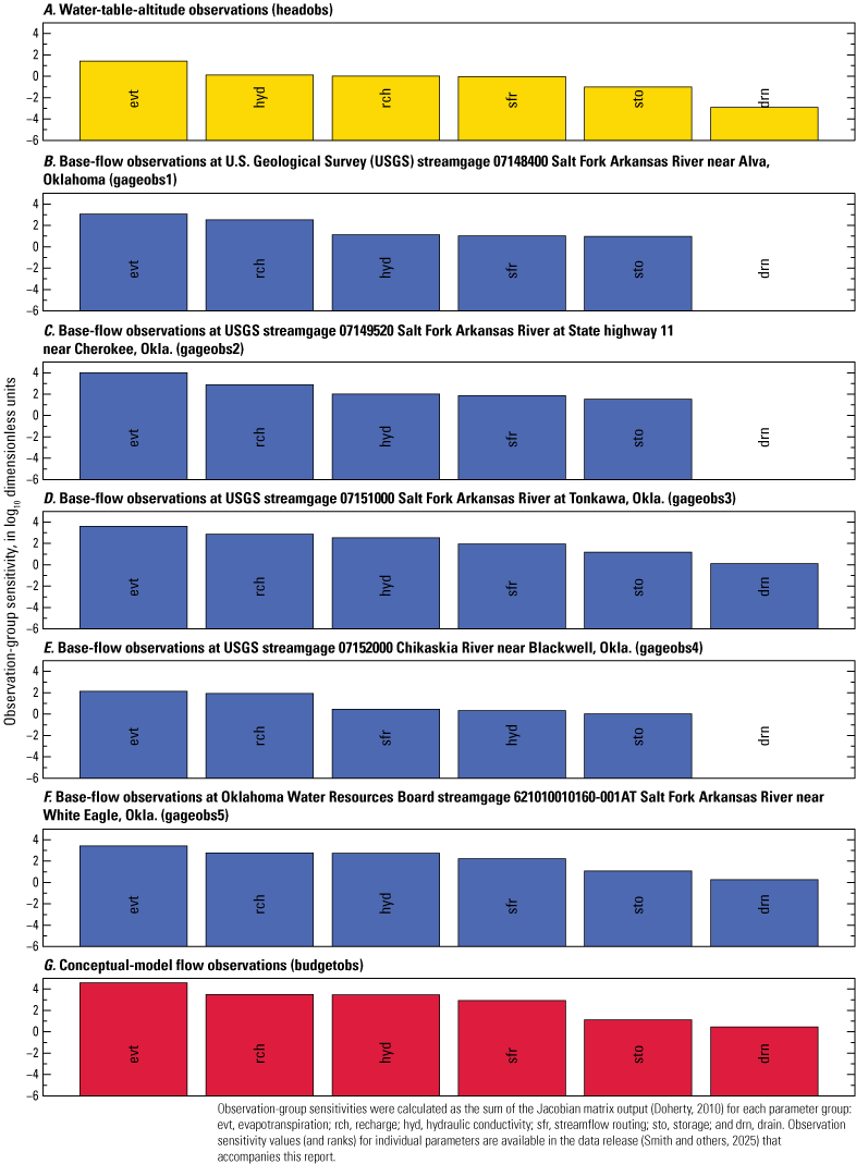
Observation-group sensitivity for calibration targets by parameter group in the numerical groundwater-flow model of the Salt Fork Arkansas River and Chikaskia River alluvial aquifers, northern Oklahoma.
Calibrated Parameter Values
The calibrated parameter values (Smith and Gammill, 2025) selected for the numerical model were the combined result of manual and automated calibration approaches. Many of the calibrated parameter values were at the minimum or maximum bounds specified in the PEST control file (Smith and Gammill, 2025), indicating that the objective function could likely be further reduced by expanding those bounds; doing so, however, would divert the numerical model further from the conceptual model or increase model instability. For the recharge parameter group (rch, table 13), 319 of 493 calibrated recharge-rate multiplier values were assigned to either the minimum or maximum bounds; 166 of those values were at the minimum bound (0.50), and 153 were at the maximum bound (2.00 for the transient multiplier values or 1.20 for the steady-state multiplier value) (Smith and Gammill, 2025). For the horizontal hydraulic conductivity parameter group (hyd, table 13), 523 of 788 calibrated parameter (pilot point) values were assigned to either the minimum or maximum bounds; 243 of those values were at the minimum bound (10.0 ft/d), and 280 were at the maximum bound (150 ft/d) (Smith and Gammill, 2025). Several of the calibrated parameter values in the evapotranspiration group (evt, table 13) were at bounds, including the steady-state saturated-zone evapotranspiration-rate multiplier, and 7 of the 12 transient (monthly) saturated-zone evapotranspiration-rate multipliers. For the streamflow-routing parameter group (sfr, table 13), all but 15 of the streambed hydraulic conductivity zone calibrated parameter values (sbk01–sbk53), all but 15 of the streambed thickness zone calibrated parameter values (sbb01–sbb53), and all but 23 of the streambed depth zone calibrated parameter values (sbd01–sbd53) were at bounds; only five of the streambed width zone calibrated parameter values were at bounds. All four storage parameter values (sy1, sy2, sy3, and ss) were at bounds; given the absence of field data on specific yield and the relative importance of that parameter in storage volume estimates, however, a uniform specific-yield value was used in the calibrated numerical model.
Comparison of Simulated and Observed Calibration Targets
Conforming to MODFLOW convention (Harbaugh, 2005), calibration-target residuals in this report were calculated as observed minus simulated values; positive residuals indicate lower simulated than observed values, and negative residuals indicate higher simulated than observed values. The mean calibrated residual for groundwater-level-altitude observations was –3.0 ft (tables 14, 15), indicating that, on average, simulated water levels were slightly higher than observed water levels. The combined (steady-state and transient simulation) groundwater-level altitude root-mean-square error was 7.8 ft, and the interquartile range was 7.3 ft (tables 14, 15; fig. 27B). When averaged by well, the mean groundwater-level altitude residuals with the greatest magnitudes mostly were associated with wells north and east of the Great Salt Plains Reservoir (fig. 28). Several wells completed in the Salt Fork Arkansas River alluvial aquifer had multiple groundwater-level altitude observations spanning multiple years of the modeling period; simulated and observed hydrographs for six of those wells (Alva; GSP2; OWRB wells 9006, 9009, 9431, and 9506) are shown in figure 27C–E (table 11, fig. 1; OWRB, 2022a; USGS, 2024).
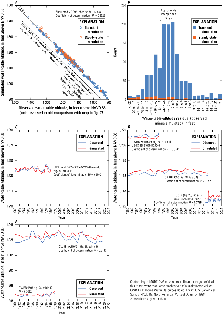
A, Relation between simulated and observed groundwater-level altitudes; B, groundwater-level-altitude residual distribution; and C–E, observed and simulated groundwater-level altitudes for selected observation wells for the numerical groundwater-flow model of the Salt Fork Arkansas River and Chikaskia River alluvial aquifers, northern Oklahoma, 1980–2020.
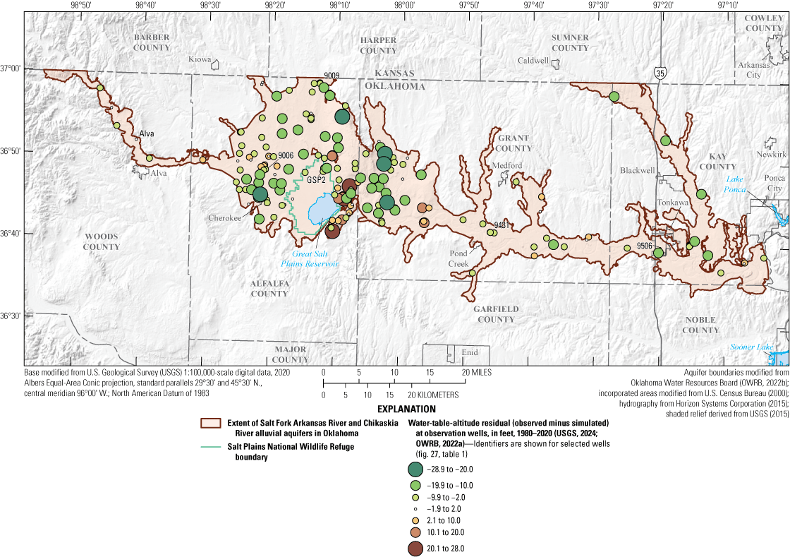
Mean groundwater-level-altitude residuals at observation wells used to calibrate the numerical groundwater-flow model of the Salt Fork Arkansas River and Chikaskia River alluvial aquifers, northern Oklahoma, 1980–2020.
The mean calibrated residuals for base-flow observations at the Tonkawa streamgage (on the Salt Fork Arkansas River), Blackwell streamgage (on the Chikaskia River), and OWRB White Eagle streamgage (on the Salt Fork Arkansas River) indicated that, on average, simulated base flows were 39.4, 42.4, and 108.1 ft3/s (tables 14, 15) lower, respectively, than the observed base flows of 412.2 of 192.2 ft3/s (tables 4, 5) and 664.8 ft3/s ([synthesized as 110 percent of the sum of 412.2 and 192.2 ft3/s], respectively). Although the model was able to match lower base flows well (fig. 29A–D), it was unable to match the highest observed base flows at these streamgages (fig. 29B–D). This mismatch is likely caused by a combination of factors, including (1) overestimation of observed base flows obtained from the BFI method, especially at the Tonkawa streamgage, which receives uncontrolled releases from the Great Salt Plains Reservoir, (2) underestimation of base-flow inflows GSPR and CHIK (fig. 22), and (3) overestimation of the scaling factor used to estimate base-flow observations at the OWRB White Eagle streamgage. The inability to simulate extreme values in the observed data is typical of groundwater-flow models (Ellis and others, 2017; Smith and others, 2017, 2021; Rogers and others, 2023) and may result from numerical-model discretization, or the necessary simplification of spatially and temporally variable hydrologic processes that occur in the physical world (Mandelbrot, 1983).
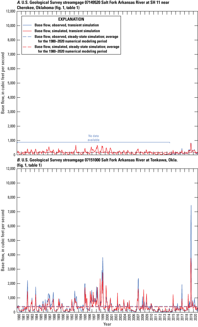
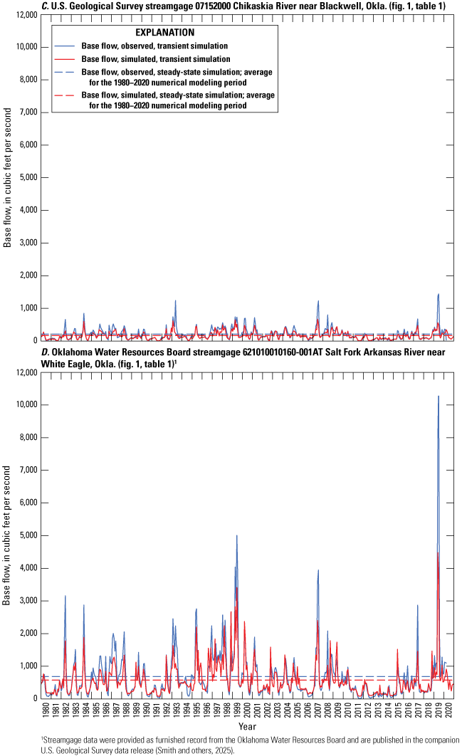
Observed base flow and simulated base flow at U.S. Geological Survey streamgages A, 07149520 Salt Fork Arkansas River at State Highway 11 near Cherokee, Oklahoma; B, 07151000 Salt Fork Arkansas River at Tonkawa, Okla.; C, 07152000 Chikaskia River near Blackwell, Okla.; and D, Oklahoma Water Resources Board streamgage 621010010160-001AT White Eagle Salt Fork Arkansas River near White Eagle, Okla., for the numerical groundwater-flow model of the Salt Fork Arkansas River and Chikaskia River alluvial aquifers, northern Oklahoma, 1980–2020.
Calibrated Numerical-Model Water Budget
The calibrated numerical-model water budget (table 16; fig. 17B) shows simulated mean annual inflows and outflows for the 1980–2020 modeling period; a subaccounting for the Chikaskia River alluvial aquifer and Salt Fork Arkansas River alluvial aquifer reaches upgradient and downgradient from the Great Salt Plains Reservoir dam was computed by using the ZONEBUDGET utility (Harbaugh, 1990). Simulated recharge (249,512 acre-ft/yr) was the only inflow for the calibrated numerical model and accounted for 100.0 percent of inflows in the water budget (table 16; fig. 17B). Net streambed seepage was the largest outflow for the calibrated numerical model, accounting for 72.3 percent of outflows in the water budget; saturated-zone evapotranspiration accounted for 20.4 percent of outflows; and well withdrawals accounted for 1.6 percent of outflows (table 16; fig. 17B). Most components of the calibrated numerical-model water budget compare well with those of the conceptual-model water budget (table 10; fig. 17). The recharge and saturated-zone evapotranspiration components, however, were greater in the calibrated numerical-model than in the conceptual-model water budget (table 10; fig. 17). These components of the conceptual model, especially the saturated-zone evapotranspiration component, were poorly constrained by available field data. No field data were available to quantify saturated-zone evapotranspiration, and effective modeling of saturated-zone evapotranspiration was outside the scope of this study. Outflows to spring seepage, net lakebed seepage, and net change in groundwater storage also were poorly constrained by available field data, but their contribution to the calibrated numerical-model budget is relatively small. Historical base-flow observations at the OWRB White Eagle streamgage on the Salt Fork Arkansas River were estimated from observations at the Tonkawa streamgage, which included uncontrolled releases from the Great Salt Plains Reservoir that could not be distinguished and separated from groundwater-derived base flows; thus, the conceptual-model net streambed seepage for the reach of the Salt Fork Arkansas River alluvial aquifer downgradient from the Great Salt Plains Reservoir may be biased high.
Table 16.
Calibrated numerical-model water budget of simulated mean annual inflows and outflows for the Salt Fork Arkansas River and Chikaskia River alluvial aquifers, 1980–2020.[All water-budget component values are in units of acre-feet per year. Totals may not equal sum of components because of independent rounding. Net water-budget totals are calculated as the difference between outflow and inflow; negative values indicate outflow from the aquifer, and positive values indicate inflow to the aquifer. Net streambed seepage, net lateral groundwater flow, and net change in groundwater storage represent the net effect of aquifer inflows and outflows. Negative net change in groundwater storage indicates gain of groundwater storage to the aquifer, which is reported as an aquifer outflow in the numerical groundwater-flow model mass balance. --, not applicable]
Simulated annual net changes in groundwater storage reflect climatic patterns during the 1980–2020 modeling period (fig. 30). Groundwater storage, for the purposes of this report, is the volume of water that would drain from the aquifer under gravity. Simulated groundwater storage was calculated by multiplying the calibrated specific yield (Smith and Gammill, 2025) by the simulated saturated thickness of each active model cell (see section “Simulated Saturated Thickness and Groundwater Storage”). The cumulative net change in simulated groundwater storage (surplus or deficit), referenced to the simulated groundwater storage at the end of the transient simulation (1,625,447 acre-ft, table 17), was between −5 and 10 percent in most years. The greatest simulated groundwater storage surplus (12.7 percent) occurred in 2007 after a year of record high recharge for the period 1980–2020. The greatest simulated groundwater storage deficit (−7.2 percent) occurred in 2012 after a year of record low recharge for the period 1980–2020. The 2012 groundwater storage deficit was fully regained by 2015, however. The transient simulation modeling period ended with a slight (1.6 percent) groundwater storage deficit (fig. 30).
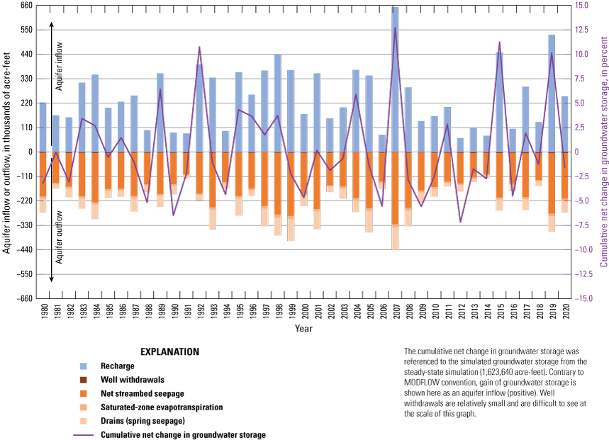
Simulated annual inflows, outflows, and cumulative net change in groundwater storage for the calibrated numerical groundwater-flow model of the Salt Fork Arkansas River and Chikaskia River alluvial aquifers, northern Oklahoma, 1980–2020.
Table 17.
Simulated hydraulic properties, storage properties, and available groundwater in storage at the end of the numerical-modeling period for the Salt Fork Arkansas River and Chikaskia River alluvial aquifers, 2020.[Kh, hydraulic conductivity; E, base-10 exponent (for example, 1.00E-04 equals 1×10⁻⁴)]
Simulated Saturated Thickness and Groundwater Storage, 2020
The simulated saturated thickness of the Salt Fork Arkansas River alluvial aquifer was determined by subtracting the altitude of the aquifer base (fig. 14) from the simulated groundwater-level altitude at the end of the modeling period (2020). The simulated saturated thickness exceeded 80 ft in the dune sand area (fig. 9) northeast of the Great Salt Plains Reservoir (fig. 31). The simulated mean thickness (defined as the sum of saturated and unsaturated thicknesses) of the Salt Fork Arkansas River alluvial aquifer was 38.86 ft (Smith and Gammill, 2025), and the simulated mean saturated thickness was 33.85 ft (table 17). The simulated mean saturated thicknesses for the Salt Fork Arkansas River alluvial aquifer reaches upgradient and downgradient from the Great Salt Plains Reservoir were 35.42 and 32.29 ft, respectively (table 17). For the Salt Fork Arkansas River alluvial aquifer, a simulated mean transmissivity of 1,962 ft2/d was calculated as the mean of the product of the calibrated horizontal hydraulic conductivity and saturated thickness for each cell. The simulated groundwater storage of the Salt Fork Arkansas River alluvial aquifer at the end of the modeling period (2020) was 1,625,447 acre-ft; of that total, 852,067 acre-ft (52.4 percent) was in the reach upgradient from the Great Salt Plains Reservoir and 773,380 acre-ft (47.6 percent) was in the reach downgradient from the reservoir (table 17). The simulated groundwater storage of the Chikaskia River alluvial aquifer was 140,789 acre-ft at the end of the modeling period (2020).
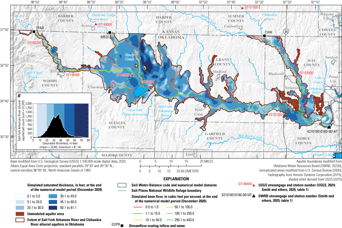
Simulated base flows and simulated saturated thickness at the end of the 1980–2020 numerical-modeling period for the calibrated numerical model of the Salt Fork Arkansas River and Chikaskia River alluvial aquifers, northern Oklahoma.
Groundwater-Availability Scenarios
Three types of groundwater-availability scenarios were evaluated by using the calibrated numerical model: 20-, 40-, and 50-year EPS scenarios, projected 50-year groundwater withdrawal scenarios, and a hypothetical 10-year drought scenario. These three types of scenarios were used to (1) estimate the EPS groundwater withdrawal rate that results in a minimum 20-, 40-, and 50-year life of the Salt Fork Arkansas River alluvial aquifer; (2) quantify the potential effects of projected well withdrawals on groundwater storage over a 50-year period; and (3) simulate the potential effects of a hypothetical 10-year drought on base flow and groundwater storage in the Salt Fork Arkansas River alluvial aquifer. The inputs and outputs for the groundwater-availability scenarios are available in Smith and Gammill (2025). The Chikaskia River alluvial aquifer was not included in the analysis and discussion of the EPS and projected 50-year groundwater withdrawal scenarios, but it was included in the numerical model to allow for that possibility in the future. However, the Chikaskia River alluvial aquifer was included in the analysis and discussion of the drought scenario, which was mostly analyzed by comparing results with those of the calibrated final model. The three groundwater-availability scenarios can help support an evaluation of the MAY for the Salt Fork Arkansas River alluvial aquifer.
Equal-Proportionate Share
EPS scenarios for the Salt Fork Arkansas River alluvial aquifer were run for periods of 20, 40, and 50 years. The 2020 simulated groundwater level from the calibrated numerical model was used as the starting groundwater level in each EPS scenario. Annual stress periods were used in these scenarios instead of monthly stress periods to simplify the analysis, improve model stability, and shorten run times. Annual model inputs for recharge, saturated-zone evapotranspiration, and stream inflows (with the exception of GSPR [fig. 22], discussed below) were assigned the means of monthly values used for each year simulated in the calibrated numerical model.
The Time-Variant Specified-Head boundary package (Harbaugh and others, 2000) representing the Great Salt Plains Reservoir was disabled for the EPS scenarios, because the shallow reservoir would quickly go dry and stop supplying water to the alluvial aquifer in an extreme groundwater withdrawal scenario. Likewise, GSPR specified inflows (fig. 22) were removed for the EPS scenarios. All simulated wells from the calibrated numerical model, including wells with prior-right permits, were discarded and replaced with a hypothetical well in every active cell, each representing about 14.7 acres. The multiplier for the altitude of the top of the aquifer was reduced to 1.00 for the EPS scenarios; these extreme groundwater withdrawal scenarios are sensitive to the aquifer top altitude, because well groundwater withdrawals are automatically reduced when the ratio of saturated thickness to aquifer thickness (aquifer top minus aquifer base altitude) approaches zero. The adjustment of specified well groundwater withdrawals is necessary because the full groundwater withdrawal rate is not possible in cells with minimal saturated thickness. The MODFLOW-2005 Well package PHIRAMP variable (Niswonger and others, 2011), which specifies the ratio of saturated thickness to aquifer thickness at which to begin reducing groundwater withdrawal rates, was set to 0.05 (5 percent of aquifer thickness) for the EPS scenarios. PEST++ (White and others, 2020), a software package for iterative parameter estimation, was used to determine the EPS groundwater withdrawal rate for the selected period (20, 40, or 50 years). In each PEST++ iteration, the hypothetical wells were assigned a uniform groundwater withdrawal rate for the selected period. If a saturated thickness of at least 5 ft was determined for more than (or less than) 50 percent of the active cells at the end of an iteration, successive iterations with an increased (or decreased) uniform groundwater withdrawal rate were performed until a saturated thickness of less than 5 ft was determined for 50 percent of the cells. To account for potential climate variability, additional EPS scenarios were run with recharge increased and decreased by 10 percent.
The Well package PHIRAMP variable (Niswonger and others, 2011) complicates the reporting of EPS groundwater withdrawal rates because the actual (reduced) EPS groundwater withdrawal rate is not uniform across cells and may be substantially less, on average, than the nominal EPS groundwater withdrawal rate specified in the Well package file (Harbaugh, 2005). The nominal and actual EPS groundwater withdrawal rates are provided in table 18 and shown on fig. 32, but only the actual EPS groundwater withdrawal rates are discussed in this section of the report. The 20-, 40-, and 50-year EPS groundwater withdrawal rates for the Salt Fork Arkansas River alluvial aquifer under normal recharge conditions were about 0.63, 0.58, and 0.57 acre-foot per acre, per year (table 18), respectively. Given the 463,838-acre modeled area of the Salt Fork Arkansas River alluvial aquifer, these EPS groundwater withdrawal rates correspond to annual yields of about 260,000–290,000 acre-ft/yr. Decreasing and increasing recharge by 10 percent resulted in about an 8- to 9-percent change in the EPS groundwater withdrawal rate (table 18). The EPS scenarios reached equilibrium (less than 0.1 percent annual change in storage) after about 35 years, so the 40- and 50-year scenarios were nearly identical (fig. 33A–C). At the end of all EPS scenarios, the simulated groundwater storage had decreased by about 74 percent, and simulated base flows on the Salt Fork Arkansas River had all substantially decreased (fig. 33). After 20 years of EPS groundwater withdrawal, the Salt Fork Arkansas River likely would be dry (less than 1.0 ft3/s) or nearly dry (1.1–10.0 ft3/s) at all locations between the Great Salt Plains Reservoir and the confluence with the Chikaskia River (figs. 33–34). Moreover, only two areas of the Salt Fork Arkansas River alluvial aquifer retained more than 5 ft of saturated thickness: (1) the high recharge area (fig. 20) corresponding to dune sand deposits (fig. 9) between Sandy Creek and Sand Creek in northeastern Alfalfa County and western Grant County, and (2) the area along streams with specified SFR2 inflows (fig. 34); areas along those simulated streams remained saturated only because they received streambed seepage inflows.
Table 18.
Equal-proportionate-share (EPS) groundwater withdrawal rates for periods of 20, 40, and 50 years for the calibrated numerical model of the Salt Fork Arkansas River alluvial aquifer, northern Oklahoma.[Results from calibrated model with no Time-Variant-Specified-Head package (Harbaugh and others, 2000) and no releases from Great Salt Plains Reservoir. All values are in units of acre-feet per acre, per year]
The MODFLOW-2005 Well package PHIRAMP variable (Niswonger and others, 2011), which specifies the ratio of saturated thickness to aquifer thickness at which to begin reducing groundwater withdrawal rates, was set to 0.05 (5 percent of aquifer thickness) for the EPS scenarios. If PHIRAMP is not specified, then a default value of 0.2 is used.
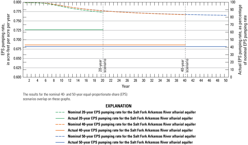
Nominal and actual equal-proportionate-share groundwater withdrawal rates for periods of 20, 40, and 50 years for the Salt Fork Arkansas River alluvial aquifer, northern Oklahoma.
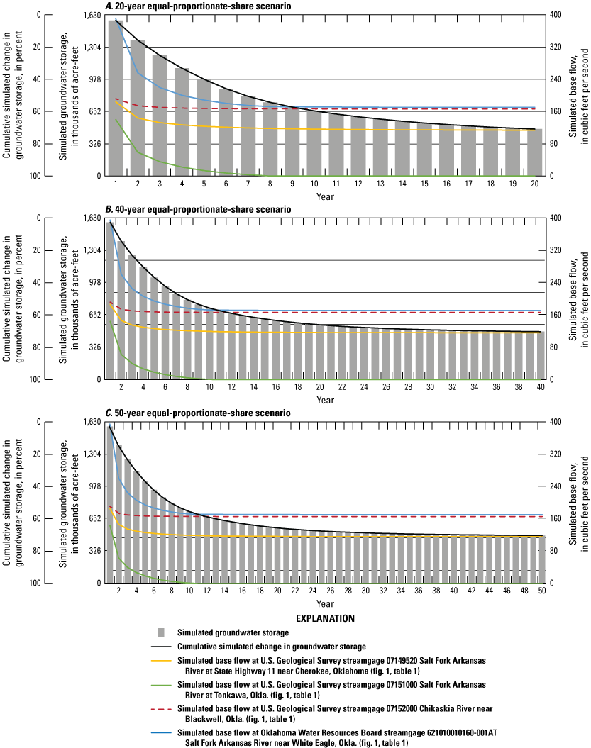
Changes in simulated base flows on the main stems of the Salt Fork Arkansas and Chikaskia Rivers and simulated groundwater storage in the Salt Fork Arkansas River alluvial aquifer, northern Oklahoma, during A, 20, B, 40, and C, 50 years of continuous equal-proportionate-share groundwater withdrawal in the Salt Fork Arkansas River alluvial aquifer, northern Oklahoma.
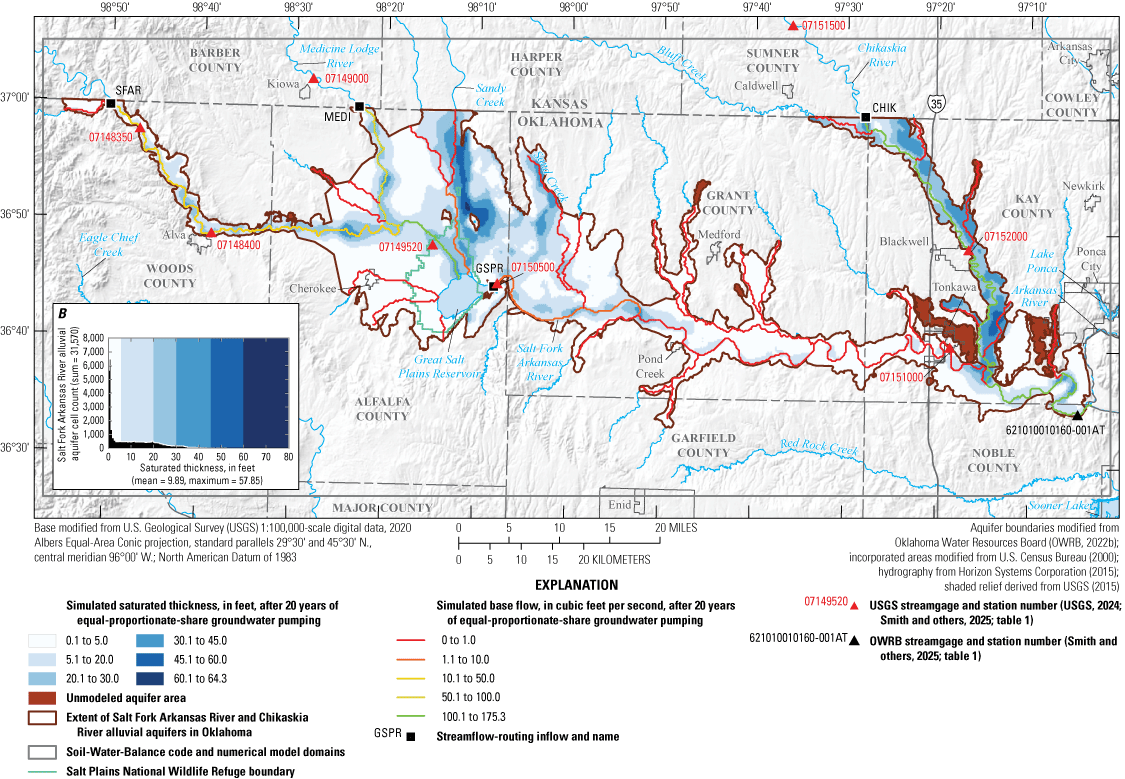
The simulated base flows and simulated saturated thickness in the Salt Fork Arkansas River and Chikaskia River alluvial aquifers after 20 years of continuous equal-proportionate-share groundwater withdrawal in the Salt Fork Arkansas River alluvial aquifer, northern Oklahoma.
EPS scenarios represent an extreme theoretical construct in which the aquifer is fully developed with regularly spaced wells (one per model cell, each representing 14.7 acres of modeled area), with each well’s groundwater withdrawal occurring at a high uniform rate. This level of development is unlikely to occur, and these EPS scenarios bear no resemblance to the current (2025) level of development in the Salt Fork Arkansas River alluvial aquifer in terms of well distribution and groundwater withdrawal rates. Some parts of the aquifer may be more developed than others, but the current level of development in the aquifer is far smaller than the level of development simulated in the EPS scenarios. Likewise, the conditions simulated in the EPS scenarios are different from the observed historical range of inflows and outflows on which the numerical model was calibrated; therefore, the results from this scenario are an extrapolation from the calibrated numerical model. The total groundwater use from the Salt Fork Arkansas River alluvial aquifer in 2020 (6,106.4 acre-ft/yr, tables 6, 7), if divided by the modeled area (463,838 acres), is equivalent to an aquifer-averaged groundwater withdrawal rate of about 0.013 acre-foot per acre, per year—less than 2 percent of the 20-year EPS groundwater withdrawal rate for the Salt Fork Arkansas River alluvial aquifer.
Projected 50-Year Groundwater Withdrawal
Projected 50-year groundwater withdrawal scenarios covering the period 2021–70 were used to simulate the effects of modified well withdrawal rates on groundwater storage in the Salt Fork Arkansas River alluvial aquifer and base flows in the Salt Fork Arkansas River. Monthly stress periods were used in these scenarios. Well withdrawals in these scenarios, unlike those in the EPS scenarios, utilized historical well withdrawal rates (or multipliers on historical well withdrawal rates) and historical well locations used in the transient simulation of the calibrated numerical model. The effects of modified well withdrawals were evaluated by quantifying differences in groundwater storage and base flow in four 50-year scenarios, which applied (1) no groundwater withdrawal, (2) mean groundwater withdrawal rates for the study period (1980–2020), (3) 2020 groundwater withdrawal rates, and (4) increasing demand groundwater withdrawal rates at simulated wells. The increasing demand groundwater withdrawal rates assumed a cumulative 45.7-percent increase (0.756-percent compounding annual increase) in groundwater withdrawal over 50 years based on 2010–60 demand projections for southern Oklahoma (OWRB, 2012b). Other monthly model inputs were assigned as the mean monthly values (for example, the mean of all January stress periods) from the calibrated numerical model and repeated for each year of the projected 50-year groundwater withdrawal scenarios; the scenarios assumed that future climate conditions were comparable to those in the 1980–2020 study period. The simulated groundwater level from the end of the calibrated numerical modeling period (2020) was used as the starting groundwater table in each of the four projected 50-year groundwater withdrawal scenarios.
Because well withdrawals were a small part of the calibrated numerical-model water budget (table 16), changes to the well groundwater withdrawal rates had little effect on simulated Salt Fork Arkansas River base flows (fig. 35) and groundwater storage (table 19) in the Salt Fork Arkansas River alluvial aquifer. For convenience of comparison, all groundwater storage changes were referenced to the groundwater storage at the end of the 2020-groundwater withdrawal-rate scenario (1,587,282 acre-ft, table 19). Groundwater storage after 50 years with no groundwater withdrawal was 1,596,164 acre-ft, or 8,882 acre-ft (0.560 percent) greater than the groundwater storage at the end of the 2020-groundwater-withdrawal-rate scenario; this groundwater storage increase is equivalent to a mean groundwater-level-altitude rise of 0.173 ft. Groundwater storage at the end of the 50-year period with the increasing demand groundwater withdrawal rates was 1,584,738 acre-ft, or 2,544 acre-ft (0.160 percent) less than the storage at the end of the 2020-groundwater-withdrawal-rate scenario; this groundwater storage decrease is equivalent to a mean groundwater-level-altitude decline of 0.050 ft. Groundwater storage after 50 years of groundwater withdrawal at the mean rate for the study period (1980–2020) was 1,588,921 acre-ft, or 1,639 acre-ft (0.103 percent) more than the groundwater storage at the end of the 2020-groundwater-withdrawal-rate scenario; this groundwater storage increase is equivalent to a mean groundwater-level-altitude rise of 0.032 ft. Although changes in groundwater storage were minimal for the model as a whole, some cells near simulated wells showed increased development of simulated cones of depression.
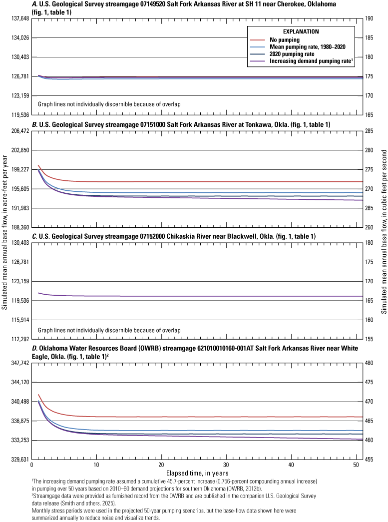
Simulated mean annual base flow at U.S. Geological Survey streamgages A, 07149520 Salt Fork Arkansas River at State Highway 11 near Cherokee, Oklahoma; B, 07151000 Salt Fork Arkansas River at Tonkawa, Okla.; C, 07152000 Chikaskia River near Blackwell, Okla.; and D, Oklahoma Water Resources Board streamgage 621010010160-001AT White Eagle Salt Fork Arkansas River near White Eagle, Okla., based on four 50-year projected groundwater withdrawal scenarios in the Salt Fork Arkansas River alluvial aquifer, northern Oklahoma.
Table 19.
Simulated changes in groundwater storage after 50 years of groundwater withdrawal at selected rates for the calibrated numerical model of the Salt Fork Arkansas River and Chikaskia River alluvial aquifers, northern Oklahoma.[Sy, specific yield]
| 50-year projected groundwater withdrawal scenario | Groundwater storage at end of 2020-groundwater- withdrawal-rate scenario (acre-feet) |
Groundwater storage at end of scenario (acre-feet) |
Change in groundwater storage (acre-feet) |
Change in groundwater storage (percent) |
Mean change in groundwater-level altitude (feet, using mean calibrated Sy of 0.1000 [table 17]) |
|---|---|---|---|---|---|
| No groundwater withdrawal | 1,587,282 | 1,596,164 | 8,882 | 0.560 | 0.173 |
| Mean groundwater withdrawal rate, 1980–2020 | 1,587,282 | 1,588,921 | 1,639 | 0.103 | 0.032 |
| 2020 groundwater withdrawal rate | 1,587,282 | 1,587,282 | 0 | 0.000 | 0.000 |
| Increasing demand groundwater withdrawal rate (cumulative 34.3-percent increase)1 | 1,587,282 | 1,584,738 | −2,544 | -0.160 | −0.050 |
The increasing demand groundwater withdrawal rate assumed a cumulative 45.7-percent increase (0.756-percent compounding annual increase) in groundwater withdrawal over 50 years based on 2010–60 demand projections for southern Oklahoma (OWRB, 2012b).
Hypothetical 10-Year Drought
A hypothetical 10-year drought scenario was used to simulate the potential effects of a prolonged period of reduced recharge on groundwater storage. The hypothetical drought period was applied to the historical period January 1983–December 1992, because that historical period had a mean annual recharge rate (5.7 in) comparable to that of the 1980–2020 study period (5.4 in., table 12); thus, scenario results were not biased to a particularly wet or dry historical period. Drought effects were quantified by comparing the results of the drought scenario to those of the calibrated numerical model (no drought) at the end of the hypothetical drought period (1992). To simulate the hypothetical drought, recharge in the calibrated numerical model was reduced by 50 percent during the hypothetical 1983–92 drought period, and inflows were reduced by 75 percent, which was comparable to the reduction in Salt Fork Arkansas River base flows at the Tonkawa streamgage during the 2010–14 drought period (fig. 6A).
Simulated groundwater storage with drought at the end of the hypothetical 10-year drought period (stress period 157) was 1,400,622 acre-ft, which is 238,283 acre-ft (14.5 percent) less than the simulated groundwater storage of the calibrated numerical model (with no drought) at the end of the drought period (1,638,905 acre-ft, fig. 36, table 20). This decrease in simulated groundwater storage is equivalent to a mean groundwater-level-altitude decline of 5.1 ft (table 20). The Salt Fork Arkansas River alluvial aquifer is more susceptible than other alluvial aquifers in Oklahoma to the effects of drought on storage and base flows because of the relatively small, saturated thickness as compared to those other alluvial aquifers (Smith and others, 2017, 2021; Ellis and others, 2020; Rogers and others, 2023). The largest simulated groundwater-level-altitude declines occurred in the terrace areas farthest upgradient from the Salt Fork Arkansas River (Smith and Gammill, 2025). The simulated saturated thickness of areas near the Salt Fork Arkansas River and its major tributaries changed little during the hypothetical drought, but the simulated base flow in streams in those areas decreased rapidly. After 12 months of the hypothetical drought, simulated base flows in the Salt Fork Arkansas River at the State Highway 11 streamgage, Tonkawa streamgage, and OWRB White Eagle streamgage and in the Chikaskia River at the Blackwell streamgage had all decreased by greater than 50 percent as compared to the calibrated numerical model (fig. 37). At the end of the hypothetical 10-year drought period (120 months), simulated base flows at the State Highway 11 streamgage, Tonkawa streamgage, Blackwell streamgage, and OWRB White Eagle streamgage had decreased by about 68, 66, 74, and 69 percent, respectively (fig. 37). After the drought period, simulated base flows mostly recovered (returned to less than a 1-percent decrease in simulated base flow) after about 5 years (fig. 37).
Table 20.
Change in simulated groundwater storage in the Salt Fork Arkansas River alluvial aquifer, northern Oklahoma, after a hypothetical 10-year drought, 1983–92.[Sy, specific yield]
| Scenario | Groundwater storage of calibrated model (with no drought) (1992) (acre-feet) | Groundwater storage at end of drought period (1992) (acre-feet) | Change in groundwater storage, 1983–92 (acre-feet) | Change in groundwater storage, 1983–92 (percent) | Mean change in groundwater-level altitude (feet, using mean calibrated Sy of 0.1000 [table 17]) |
|---|---|---|---|---|---|
| Hypothetical 10-year drought | 1,638,905 | 1,400,622 | 238,283 | 14.5 | 5.1 |
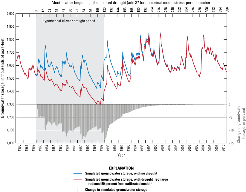
Simulated groundwater storage with drought, simulated groundwater storage with no drought, and changes in simulated groundwater storage resulting from a hypothetical 10-year drought (1983–92) for the Salt Fork Arkansas River alluvial aquifer, northern Oklahoma, 1980–2010.
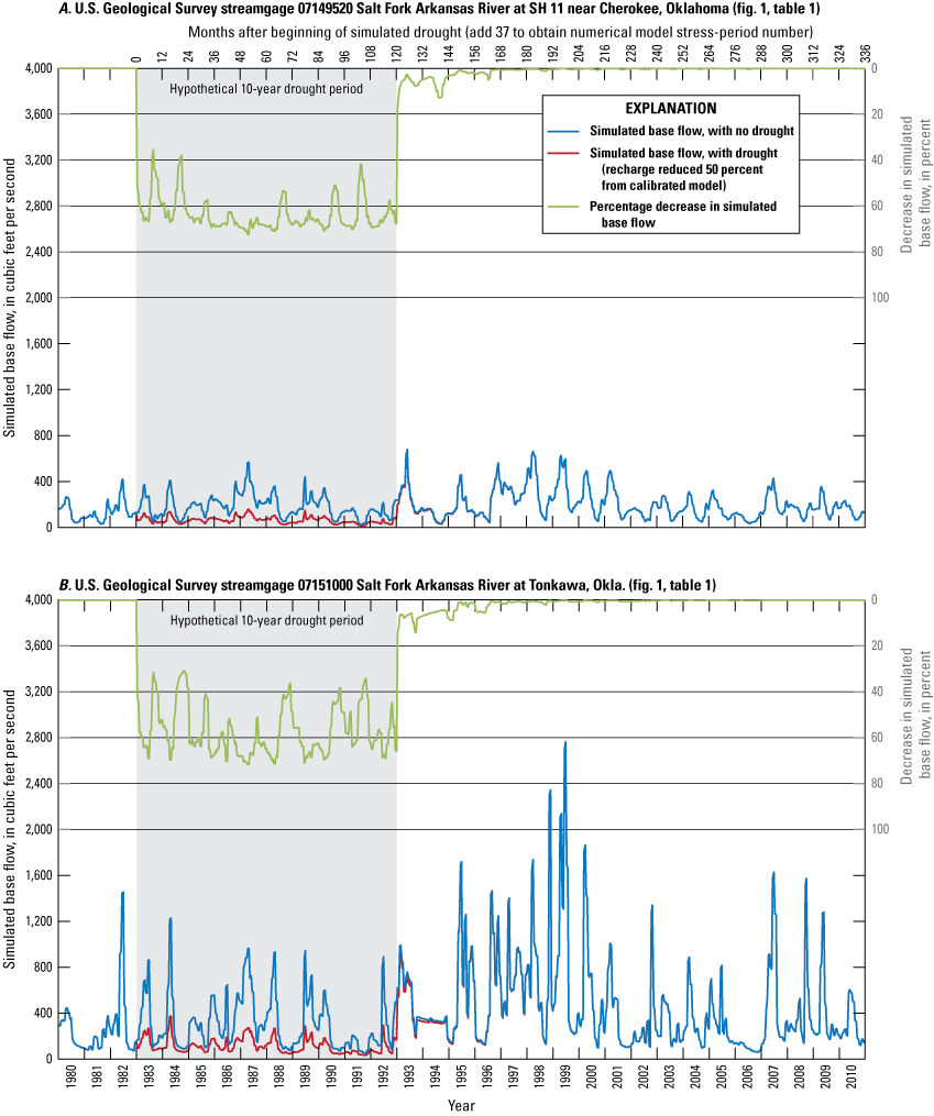
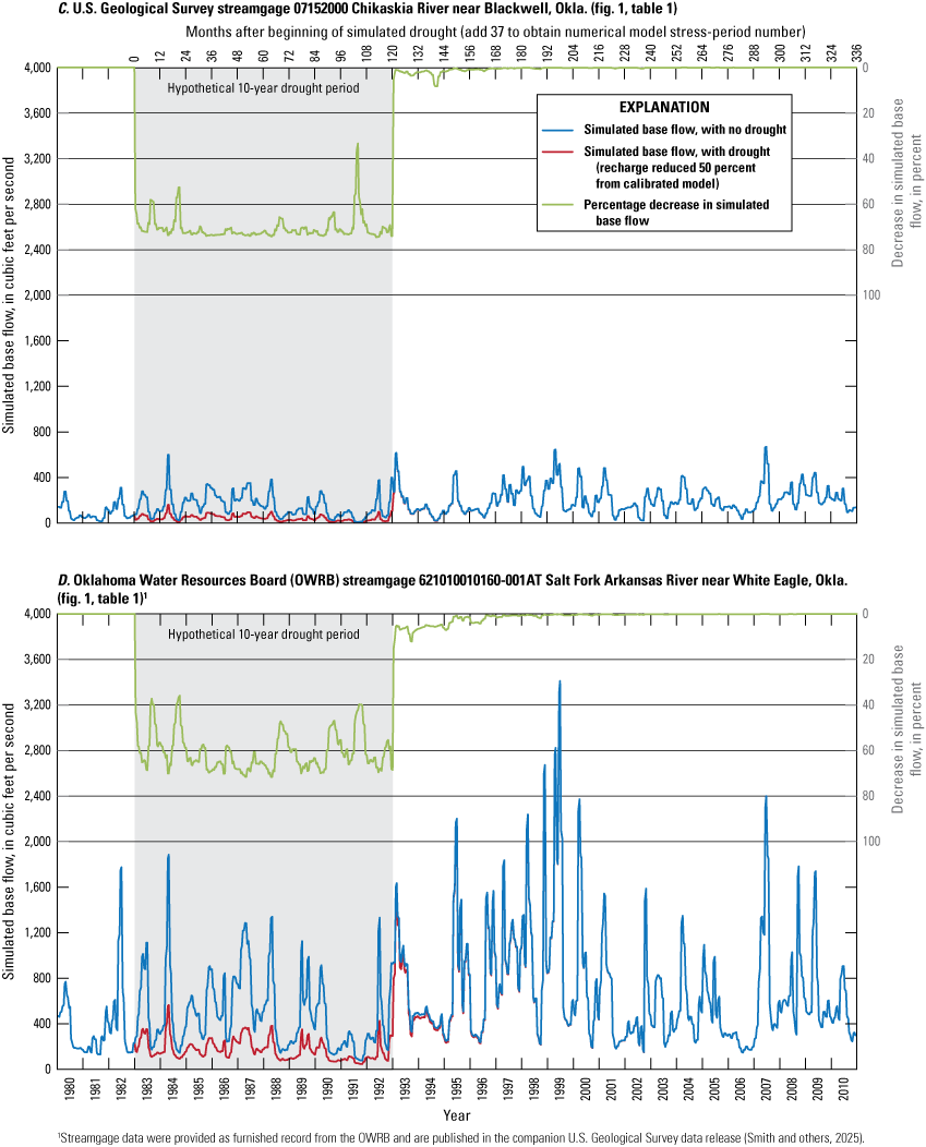
Simulated base flows with drought, simulated base flows with no drought, and changes in simulated base flows at U.S. Geological Survey streamgages A, 07149520 Salt Fork Arkansas River at State Highway 11 near Cherokee, Oklahoma; B, 07151000 Salt Fork Arkansas River at Tonkawa, Okla.; C, 07152000 Chikaskia River near Blackwell, Okla.; and D, Oklahoma Water Resources Board streamgage 621010010160-001AT White Eagle Salt Fork Arkansas River near White Eagle, Okla., resulting from a hypothetical 10-year drought (1983–92) for the Salt Fork Arkansas River and Chikaskia River alluvial aquifers, northern Oklahoma, 1980–2010.
Model Limitations
Some assumptions and simplifications were necessary in the simulation of groundwater flow in the calibrated numerical model. The use of the MODFLOW code requires the assumptions that groundwater flows are governed by Darcy’s Law (Darcy, 1856), water is incompressible and of uniform density, and the aquifer hydrogeology can be simulated appropriately by the cell size and number of layers present. Computing and time limitations and low-input data densities (that is, data that are relatively sparse spatially, vertically, or temporally) prevented the use of cell sizes that could better represent the true variability of the hydrogeologic characteristics of the aquifer; therefore, results generated by the model may be more applicable to a regional, rather than local, area. No groundwater-level-altitude observations were available for the beginning of the modeling period (1980), so the steady-state simulation was calibrated to mean groundwater-level-altitude observations from the transient period at each observation well. Uneven temporal and spatial distributions of groundwater-level-altitude observations caused data gaps in the calibration data (figs. 26, 29), which can reduce confidence in model results for those times and areas. Additionally, base flow is based on the simulated groundwater level and may not be accurately represented in locations where groundwater-level-altitude observation data were relatively sparse.
The edges of most of the modeled area, including the bottoms of active cells, were simulated as no-flow boundaries. This practice is common in numerical-model simulations, but it is a simplification that, given the large number of cells involved, likely adds uncertainty to the results described in this report. The stream network used in the numerical model is also a simplification of the actual stream geometry and hydraulic properties. Refined measurement of the stream channel width and streambed conductivity at the local scale could improve the numerical-model calibration because these factors control the amount of streambed seepage exchange with the aquifer. The numerical model was calibrated primarily to base-flow estimates; therefore, additional streamflow data that represent other hydrologic conditions could help further reduce uncertainty in local-scale simulation results.
The specific-yield value, which acts as a multiplier on aquifer storage, was not constrained by any field data from the Salt Fork Arkansas River or Chikaskia River alluvial aquifers, and the initial specific-yield values were obtained from nine multiwell aquifer tests documented by Reed and others (1952). Additional measurements of specific yield obtained from aquifer tests in the study area could improve the numerical model calibration. However, the specific-yield value (0.1000) ultimately used in the calibrated numerical model was within the range of specific-yield values used in other alluvial aquifer models for Oklahoma (Ellis and others, 2020; Smith and others, 2021; Rogers and others, 2023).
No historical streamflow data were available from the most downstream part of the study area, so streambed seepage data were estimated using a scaling factor. No field data were available to quantify saturated-zone evapotranspiration. Exact amounts of annual groundwater use are unknown because groundwater wells are not metered, and reported groundwater-use data are based on estimates of varying quality submitted to the OWRB by permit holders. Additionally, groundwater use for domestic supply, though assumed to be relatively small, was not included in the numerical model.
Summary
The 1973 Oklahoma Groundwater Law (Oklahoma Statute §82–1020.5) requires that the Oklahoma Water Resources Board (OWRB) conduct hydrologic investigations of the State’s aquifers to determine the maximum annual yield (MAY) for each groundwater basin. The MAY is defined as the total amount of fresh groundwater that can be annually withdrawn while allowing a minimum 20-year life of that groundwater basin. The equal-proportionate-share (EPS) groundwater withdrawal rate is defined as the annual volume of groundwater allocated per acre of land. The U.S. Geological Survey (USGS), in cooperation with the OWRB, conducted an updated hydrologic investigation of the Salt Fork Arkansas River and Chikaskia River alluvial aquifers in northern Oklahoma for a study period spanning 1980–2020 and evaluated the simulated effects of potential groundwater withdrawals on groundwater flow and availability in the Salt Fork Arkansas River alluvial aquifer to support the OWRB’s evaluation of the MAY for that aquifer. The conceptual-model and numerical-model aquifer area totaled 512,808 acres.
The purpose of this report is to describe a hydrologic investigation of the Salt Fork Arkansas River and Chikaskia River alluvial aquifers in northern Oklahoma. This description included (1) a summary of the hydrogeology with a definition of a hydrogeologic framework of the aquifer, (2) development of conceptual and calibrated numerical groundwater-flow models for the aquifer representing the 1980–2020 study period, and (3) results of simulations of groundwater-availability scenarios. The calibrated numerical groundwater-flow model and groundwater availability scenarios were archived and released in a USGS data release.
A groundwater-hydrograph-based water-table-fluctuation (WTF) method was used to estimate localized annual recharge rates. Groundwater-level hydrographs from seven USGS continuous-recorder wells in the Salt Fork Arkansas River alluvial aquifer were used to estimate annual recharge for 1981–95 and 2019–21. The resulting WTF annual recharge estimates were normalized by the mean annual precipitation for the study period 1980–2020 and averaged; the resulting mean annual recharge value for the period of record was 5.4 inches (in.), or 16.3 percent of mean annual precipitation for the period 1980–2020. Multiplied by the 512,808-acre total aquifer area and unit converted, the WTF-calculated mean annual recharge for both aquifers was 230,764 acre-feet (acre-ft); this value was used for the conceptual model recharge 1980–2020.
The Soil-Water-Balance code was calibrated to the WTF-calculated mean annual recharge and used to estimate spatially distributed recharge rates. The Soil-Water-Balance code-estimated mean annual recharge values for the 1980–2020 study period were 5.13 in. (15.5 percent of the mean annual precipitation of 33.1 in. during 1980–2020) for the Salt Fork Arkansas River alluvial aquifer and 3.57 in. (10.8 percent of the mean annual precipitation of 33.1 in. during 1980–2020) for the Chikaskia River alluvial aquifer. Spatially, mean annual recharge for the study period was greatest in windblown dune sands northwest of the Great Salt Plains Reservoir and in areas of active alluvium near the Salt Fork Arkansas River and tributaries.
The numerical groundwater-flow model of the Salt Fork Arkansas River and Chikaskia River alluvial aquifers was constructed by using the USGS modular groundwater-flow model MODFLOW-2005 with the Newton formulation solver. The model domain of the Salt Fork Arkansas River and Chikaskia River alluvial aquifers was spatially discretized into 300 rows, 700 columns, 34,903 active cells (31,570 and 3,333 active cells for the Salt Fork Arkansas River and Chikaskia River alluvial aquifers, respectively) measuring 800 by 800 feet (ft) each, and a single convertible layer based on the hydrogeologic framework described in this report. The numerical model was temporally discretized into 492 monthly transient stress periods (each with two time steps to improve model stability) representing the 1980–2020 study period. An initial steady-state stress period represented mean annual inflows to, and outflows from, the aquifer. The steady-state solution was used as the initial condition for subsequent transient stress periods, as well as some groundwater-availability scenarios. The numerical model was calibrated to groundwater-level-altitude observations at selected wells, base-flow observations at selected streamgages, and selected components of a conceptual-model water budget.
The simulated saturated thickness exceeded 80 ft in the dune sand area northeast of the Great Salt Plains Reservoir. The simulated mean thickness (sum of saturated and unsaturated thicknesses) of the Salt Fork Arkansas River alluvial aquifer was 38.86 ft, and the simulated mean saturated thickness was 33.85 ft. The simulated mean saturated thicknesses for the Salt Fork Arkansas River alluvial aquifer reaches upgradient and downgradient from the Great Salt Plains Reservoir were 35.42 and 32.29 ft, respectively. For the Salt Fork Arkansas River alluvial aquifer, a simulated mean transmissivity of 1,962 square feet per day was calculated as the mean of the calibrated horizontal hydraulic conductivity multiplied by the saturated thickness of each cell. The simulated groundwater storage of the Salt Fork Arkansas River alluvial aquifer at the end of the modeling period (2020) was 1,625,447 acre-ft; 852,067 acre-ft (52.4 percent) of that total was in the reach upgradient from the Great Salt Plains Reservoir, and 773,380 acre-ft (47.6 percent) of that total was in the reach downgradient from the Great Salt Plains Reservoir. The simulated groundwater storage of the Chikaskia River alluvial aquifer at the end of the modeling period (2020) was 140,789 acre-ft.
Three types of groundwater-availability scenarios were evaluated by using the calibrated numerical model: 20-, 40-, and 50-year EPS scenarios, projected 50-year groundwater withdrawal scenarios, and a hypothetical 10-year drought scenario. The three types of scenarios were limited to the Salt Fork Arkansas River alluvial aquifer. The 20-, 40-, and 50-year EPS groundwater withdrawal rates for the Salt Fork Arkansas River alluvial aquifer under normal recharge conditions were about 0.63, 0.58, and 0.57 acre-foot per acre, per year, respectively. Given the 463,838-acre modeled area of the Salt Fork Arkansas River alluvial aquifer, these EPS groundwater withdrawal rates correspond to annual yields of about 260,000–290,000 acre-feet per year. Decreasing and increasing recharge by 10 percent resulted in about an 8- to 9-percent change in the EPS groundwater withdrawal rate. The EPS scenarios reached equilibrium (less than 0.1 percent annual change in storage) after 35 years, which resulted in nearly identical 40- and 50-year scenarios. At the end of all EPS scenarios, the simulated groundwater storage had decreased by 74 percent, and simulated base flows on the Salt Fork Arkansas River had all substantially decreased. After 20 years of EPS groundwater withdrawal, the Salt Fork Arkansas River likely would be dry (less than 1.0 cubic feet per second) or nearly dry (1.1–10.0 cubic feet per second) at all locations between the Great Salt Plains Reservoir and the confluence with the Chikaskia River. After 20 years of EPS groundwater withdrawal, only areas along streams with specified SFR2 inflows retained more than 5 ft of saturated thickness; areas along those streams remained saturated only because they received streambed seepage. Projected 50-year groundwater withdrawal scenarios were used to simulate the effects of modified well withdrawal rates on groundwater storage in the Salt Fork Arkansas River alluvial aquifer and base flows in the Salt Fork Arkansas River. The effects of modified well withdrawals were evaluated by quantifying differences in groundwater storage and base flow in four 50-year scenarios, which applied (1) no groundwater withdrawal, (2) 2020 groundwater withdrawal rates, (3) projected increasing demand groundwater withdrawal rates at simulated wells, and (4) mean groundwater withdrawal rates for the study period (1980–2020). Because well withdrawals were a small part of the calibrated numerical-model water budget, changes to the well groundwater withdrawal rates had little effect on simulated Salt Fork Arkansas River base flows or groundwater storage in the Salt Fork Arkansas River alluvial aquifer. A hypothetical 10-year drought scenario was used to simulate the potential effects of a prolonged period of reduced recharge on groundwater storage. January 1983– December 1992 was chosen as the hypothetical drought period because it had a mean annual recharge rate (5.7 in) comparable to that of the 1980–2020 study period. Drought effects were quantified by comparing the results of the drought scenario to those of the calibrated numerical model (no drought) at the end of the hypothetical drought period (1992). To simulate the hypothetical drought, recharge in the calibrated numerical model was reduced by 50 percent during the hypothetical drought period (1983–92), and inflows were reduced by 75 percent, which was comparable to the reduction in Salt Fork Arkansas River base flows at the Tonkawa streamgage during the 2010–14 drought period.
Simulated groundwater storage with drought at the end of the hypothetical 10-year drought period (stress period 157) was 1,400,622 acre-ft, which is 238,283 acre-ft (14.5 percent) less than the simulated groundwater storage of the calibrated numerical model (with no drought) at the end of the drought period (1,638,905 acre-ft). This decrease in simulated groundwater storage is equivalent to a mean groundwater-level-altitude decline of 5.1 ft. Because of its relatively small, saturated thickness, the Salt Fork Arkansas River alluvial aquifer can be more susceptible to the effects of drought on storage and base flows as compared to other alluvial aquifers in Oklahoma. The largest simulated groundwater-level-altitude declines occurred in the terrace areas most upgradient from the Salt Fork Arkansas River. The simulated saturated thickness of areas near the Salt Fork Arkansas River and its major tributaries changed little during the hypothetical drought, but the simulated base flow in streams in those areas decreased rapidly. At the end of the hypothetical 10-year drought period (120 months), simulated base flows at the State Highway 11 streamgage, Tonkawa streamgage, Blackwell streamgage, and OWRB White Eagle streamgage had decreased by about 68, 66, 74, and 69 percent, respectively. After the drought period, simulated base flows mostly recovered, returning to less than a 1-percent decrease in simulated base flow, after about 5 years.
References Cited
Arnold, J.G., Muttiah, R.S., Srinivasan, R., and Allen, P.M., 2000, Regional estimation of base flow and groundwater recharge in the Upper Mississippi River Basin: Journal of Hydrology, v. 227, nos. 1–4, p. 21–40, accessed April 15, 2024, at https://doi.org/10.1016/S0022-1694(99)00139-0.
Barlow, P.M., Cunningham, W.L., Zhai, T., and Gray, M., 2015, U.S. Geological Survey groundwater toolbox, a graphical and mapping interface for analysis of hydrologic data (version 1.0)—User guide for estimation of base flow, runoff, and groundwater recharge from streamflow data: U.S. Geological Survey Techniques and Methods, book 3, chap. B10, 27 p., accessed June 5, 2020, at https://doi.org/10.3133/tm3B10.
Barlow, P.M., and Leake, S.A., 2012, Streamflow depletion by wells—Understanding and managing the effects of groundwater pumping on streamflow: U.S. Geological Survey Circular 1376, 84 p., accessed June 5, 2020, at https://doi.org/10.3133/cir1376.
Belden, M., 1997, Hydrologic report of the minor groundwater basins in Garfield, Grant and Kay Counties: Oklahoma Water Resources Board, Planning and Management Division Technical Report, v. 97, no. 4, 24 p., accessed September 14, 2023, at https://www.owrb.ok.gov/studies/reports/reports_pdf/TR97_4%20Minor%20GW%20Basins%20Garfield%20Grant%20Kay%20-%20North%20Central%20and%20Chikaskia.pdf.
Bennett, G.D., 1976, Introduction to ground-water hydraulics, a programmed text for self-instruction: U.S. Geological Survey Techniques of Water-Resources Investigations, book 3, chap. B2, 172 p., accessed July 21, 2022, at https://doi.org/10.3133/twri03B2.
Bingham, R.H., and Bergman, D.L., 1980, Reconnaissance of the water resources of the Enid quadrangle, north-central Oklahoma: Oklahoma Geological Survey Hydrologic Atlas 7, 4 sheets, scale 1:250,000, accessed July 24, 2022, at https://www.ou.edu/ogs/maps/hydrologicatlases.
Cleveland, W., 1979, Robust locally weighted regression and smoothing scatterplots: Journal of the American Statistical Association, v. 74, no. 368, p. 829–836, accessed August 4, 2022, at https://doi.org/10.1080/01621459.1979.10481038.
Cowardin, L.M., Carter, V., Golet, F.C., and LaRoe, E.T., 1979, Classification of wetlands and deepwater habitats of the United States: Washington, D.C., U.S. Fish and Wildlife Service, FWS/OBS–79/31, 131 p., accessed July 21, 2022, at https://www.fws.gov/media/classification-wetlands-and-deepwater-habitats-united-states-0.
Cunningham, W.L., and Schalk, C.W., 2011, Groundwater technical procedures of the U.S. Geological Survey: U.S. Geological Survey Techniques and Methods, book 1, chap. A1, 151 p., accessed June 5, 2020, at https://doi.org/10.3133/tm1A1.
Davis, J.L., 1968, Meteorologic and hydrologic relationships on the Great Salt Plains of Oklahoma: Oklahoma Geology Notes, v. 28, no. 5, p. 163–168, accessed August 8, 2022, at http://ogs.ou.edu/docs/geologynotes/GN-V28N5.pdf.
Doherty, J., 2010, PEST, model independent parameter estimation user manual (5th ed., ver. 18): Brisbane, Australia, Watermark Numerical Computing, accessed August 3, 2022, at https://pesthomepage.org/programs.
Dover, T.B., 1957, Water quality—A factor in Arkansas River development: U.S. Geological Survey Open-File Report 57–40, 14 p., accessed August 26, 2024, at https://pubs.usgs.gov/publication/ofr5740.
Dover, T.B., Leonard, A.R., and Laine, L.L., 1968, Water for Oklahoma: U.S. Geological Survey Water-Supply Paper 1890, 107 p., accessed July 23, 2020, at https://books.google.com/books?hl=en&lr=&id=NVr834zaDbsC&oi=fnd&pg=PA1&dq=dover+1957+salt+fork&ots=KMKlqcOM9E&sig=xDo-fU_lPoLK_a4iM4goMPrGSYg#v=onepag e&q&f=false.
Eckenstein, E., 1994, Surface-groundwater study of the alluvium and terrace aquifer of the Salt Fork of the Arkansas River and saline surface water in north Oklahoma: Oklahoma Water Resources Board, FY 92 106 Groundwater Task 410, 44 p., accessed January 4, 2021, at https://www.owrb.ok.gov/studies/reports/reports_pdf/Study%20of%20the%20Aquifer%20of%20the%20Salt%20Fork%20Arkansas%20River.pdf.
Eckenstein, E., 1995, Sensitivity of the alluvial and terrace-alluvial aquifer of the Salt Fork of the Arkansas River to induced infiltration: Stillwater, Okla., Oklahoma State University, master’s thesis, 69 p., accessed August 3, 2022, at https://openresearch.okstate.edu/bitstreams/81ed2c5d-45aa-4b16-b50e-a6dc9e05f2ac/download.
Ellis, J.H., 2018, Simulation of groundwater flow and analysis of projected water use for the Rush Springs aquifer, western Oklahoma: U.S. Geological Survey Scientific Investigations Report 2018–5136, 156 p., accessed March 1, 2019, at https://doi.org/10.3133/sir20185136.
Ellis, J.H., Mashburn, S.L., Graves, G.M., Peterson, S.M., Smith, S.J., Fuhrig, L.F., Wagner, D.L., and Sanford, J.E., 2017, Hydrogeology and simulation of groundwater flow and analysis of projected water use for the Canadian River alluvial aquifer, western and central Oklahoma: U.S. Geological Survey Scientific Investigations Report 2016–5180, 64 p., accessed August 2, 2022, at https://doi.org/10.3133/sir20165180.
Ellis, J.H., Ryter, D.W., Fuhrig, L.T., Spears, K.W., Mashburn, S.L., and Rogers, I.M.J., 2020, Hydrogeology, numerical simulation of groundwater flow, and effects of future water use and drought for reach 1 of the Washita River alluvial aquifer, Roger Mills and Custer Counties, western Oklahoma, 1980–2015: U.S. Geological Survey Scientific Investigations Report 2020–5118, 81 p., accessed August 3, 2022, at https://doi.org/10.3133/sir20205118.
Esri, 2021a, ArcGIS for desktop help—Fill tool: Esri web page, accessed May 6, 2021, at https://desktop.arcgis.com/en/arcmap/10.7/tools/spatial-analyst-toolbox/fill.htm.
Esri, 2021b, ArcGIS for desktop help—IDW tool: Esri web page, accessed May 6, 2021, at https://desktop.arcgis.com/en/arcmap/10.7/tools/spatial-analyst-toolbox/idw.htm.
Fader, S.W., and Morton, R.B., 1975, Ground water in the middle Arkansas River Basin, Kansas and Oklahoma: U.S. Geological Survey Open-File Report 75–367, 44 p., accessed July 22, 2022, at https://doi.org/10.3133/ofr75367.
Fry, J.A., Xian, G., Jin, S., Dewitz, J.A., Homer, C.G., Yang, L., Barnes, C.A., Herold, N.D., and Wickham, J.D., 2011, Completion of the 2006 National Land Cover Database for the conterminous United States: Photogrammetric Engineering and Remote Sensing, v. 77, no. 9, p. 858–864, accessed August 4, 2019, at https://pubs.usgs.gov/publication/70034549.
Garner, B.D., and Bills, D.J., 2012, Spatial and seasonal variability of base flow in the Verde Valley, central Arizona, 2007 and 2011: U.S. Geological Survey Scientific Investigations Report 2012–5192, 33 p., accessed August 4, 2022, at https://doi.org/10.3133/sir20125192.
Geoprobe Systems, 2015, Geoprobe Hydraulic Profiling Tool (HPT) system, standard operating procedure: Salina, Kans., Kejr, Inc., Technical Bulletin MK3137, 22 p., accessed March 14, 2017, at https://geoprobe.com/literature/hpt-sop.
Geoprobe Systems, 2020, Direct Image Viewer user guide (revision 2.0, April 2020): Salina, Kans., Kejr, Inc., 40 p., accessed July 31, 2020, at https://geoprobe.com/sites/default/files/storage/pdfs/DI%20Viewer%20User%20Guide%20Rev.2.0.pdf.
Gomo, M., 2011, A groundwater-surface water interaction study of an alluvial channel aquifer: Bloemfontein, South Africa, University of the Free State, Ph.D. dissertation, 201 p., accessed September 20, 2024, at https://scholar.ufs.ac.za/server/api/core/bitstreams/2db68146-56ee-474a-aa7f-9cc191e336e5/content.
Guy, H.P., 1969, Laboratory theory and methods for sediment analysis: U.S. Geological Survey Techniques of Water-Resources Investigations, book 5, chap. C1, 58 p., accessed August 28, 2020, at https://doi.org/10.3133/twri05C1.
Harbaugh, A.W., 1990, A computer program for calculating subregional water budgets using results from the U.S. Geological Survey modular three-dimensional groundwater-flow model: U.S. Geological Survey Open-File Report 90–392, 46 p., accessed June 5, 2020, at https://doi.org/10.3133/ofr90392.
Harbaugh, A.W., 2005, MODFLOW-2005, the U.S. Geological Survey modular ground-water model—The Ground-Water Flow Process: U.S. Geological Survey Techniques and Methods, book 6, chap. A16, 253 p., accessed May 30, 2020, at https://doi.org/10.3133/tm6A16.
Harbaugh, A.W., Banta, E.R., Hill, M.C., and McDonald, M.G., 2000, MODFLOW-2000, the U.S. Geological Survey modular ground-water model—User guide to modularization concepts and the ground-water flow process: U.S. Geological Survey Open-File Report 2000–92, 121 p., accessed August 3, 2022, at https://doi.org/10.3133/ofr200092.
Hargreaves, G.H., and Samani, Z.A., 1985, Reference crop evapotranspiration from temperature: Applied Engineering in Agriculture, v. 1, no. 2, p. 96–99, accessed August 3, 2022, at https://doi.org/10.13031/2013.26773.
Healy, R.W., and Cook, P.G., 2002, Using groundwater levels to estimate recharge: Hydrogeology Journal, v. 10, no. 1, p. 91–109, accessed August 3, 2022, at https://doi.org/10.1007/s10040-001-0178-0.
Heath, R.C., 1983, Basic ground-water hydrology: U.S. Geological Survey Water-Supply Paper 2220, 84 p., accessed August 27, 2020, at https://doi.org/10.3133/wsp2220.
Helsel, D.R., Hirsch, R.M., Ryberg, K.R., Archfield, S.A., and Gilroy, E.J., 2020, Statistical methods in water resources: U.S. Geological Survey Techniques and Methods, book 4, chap. A3, 458 p., accessed August 19, 2024, at https://doi.org/10.3133/tm4A3. [Supersedes USGS Techniques of Water-Resources Investigations, book 4, chap. A3, version 1.1.]
Hem, J.D., 1985, Study and interpretation of the chemical characteristics of natural water (3d ed.): U.S. Geological Survey Water-Supply Paper 2254, 263 p., accessed August 23, 2022, at https://doi.org/10.3133/wsp2254.
Hill, M.C., Banta, E.R., Harbaugh, A.W., and Anderman, E.R., 2000, MODFLOW-2000, the U.S. Geological Survey modular ground-water model—User guide to the observation, sensitivity, and parameter-estimation processes and three post-processing programs: U.S. Geological Survey Open-File Report 00–184, 210 p., accessed June 5, 2020, at https://doi.org/10.3133/ofr00184.
Horizon Systems Corporation, 2015, National Hydrography Dataset Plus (NHDPlus) version 2: Horizon Systems Corporation database, accessed August 3, 2022, at https://nhdplus.com/NHDPlus/.
In-Situ, Inc., 2023, Level TROLL 400, 500 & 700 data loggers [specifications sheet]: Fort Collins, Colo., In-Situ, Inc., 2 p., accessed December 15, 2023, at https://in-situ.com/pub/media/support/documents/LevelTROLL_Spec-Sheet_ltr_en_0723.pdf.
Johnson, K.S., 2022, Salt Plains and brines in western Oklahoma—Results from dissolution of Permian salt and distinguishing those brines from oil-field brines: Oklahoma Geological Survey Bulletin 153, 73 p., accessed April 4, 2024, at https://www.ou.edu/content/dam/ogs/documents/bulletins/Bulletin%20153.pdf.
Jordan, L., and Vosburg, D., 1963, Permian salt and associated evaporites in the Anadarko Basin of the western Oklahoma-Texas Panhandle region: Oklahoma Geological Survey Bulletin 102, 76 p., accessed January 11, 2021, at http://www.ogs.ou.edu/pubsscanned/BULLETINS/Bulletin102mm.pdf.
Kendall, M.G., 1938, A new measure of rank correlation: Biometrika, v. 30, nos. 1–2, p. 81–93, accessed August 3, 2022, at https://doi.org/10.1093/biomet/30.1-2.81.
Koller, M., Chatelain, J.L., Guiltier, B., Duval, A.M., Atakan, K., Lacave, C., and Bard, P.Y., 2004, Practical user guidelines and software for the implementation of the H/V ratio technique—Measuring conditions, processing method and results interpretation in 13th World Conference on Earthquake Engineering, Vancouver, British Columbia, Canada, August 16, 2004, [Proceedings]: International Association for Earthquake Engineering, SESAME Project Team, World Conference on Earthquake Engineering, Paper No. 3132, accessed April 23, 2020, at https://citeseerx.ist.psu.edu/viewdoc/download?doi=10.1.1.626.6948&rep=rep1&type=pdf.
Lubczynski, M.W., 2009, The hydrogeological role of trees in water-limited environments: Hydrogeology Journal, v. 17, no. 1, p. 247–259, accessed June 5, 2020, at https://doi.org/10.1007/s10040-008-0357-3.
Mandelbrot, B.B., 1983, The fractal geometry of nature: New York, W.H. Freeman, 468 p. [Also available at https://doi.org/10.1119/1.13295.]
Mashburn, S.L., Ryter, D.W., Neel, C.R., Smith, S.J., and Correll, J.S., 2018, Hydrogeology and simulation of groundwater flow in the Central Oklahoma (Garber-Wellington) aquifer, Oklahoma, 1987 to 2009, and simulation of available water in storage, 2010–2059: U.S. Geological Survey Scientific Investigations Report 2013–5219, 92 p., accessed June 5, 2020, at https://doi.org/10.3133/sir20135219.
McCall, W., 2010, Tech guide for calculation of estimated hydraulic conductivity (Est. K) log from HPT data: Salina, Kans., Kejr, Inc., 20 p., accessed August 3, 2022, at https://geoprobe.com/sites/default/files/pdfs/tech_guide_estk_v5_0_0.pdf.
Microsoft Corporation, 2022, Bing Maps imagery API: Microsoft web page, accessed May 30, 2022, at https://learn.microsoft.com/en-us/bingmaps/rest-services/imagery/.
Miller, G.W., and Stanley, T.M., 2003, Geologic map of the Alva 30' X 60' quadrangle, Alfalfa, Grant, Major, Woods, and Woodward Counties, Oklahoma: Oklahoma Geological Survey Geologic Quadrangle Map OGQ–42, 1 sheet, scale 1:100,000, accessed February 4, 2022, at http://ogs.ou.edu/docs/OGQ/OGQ-42-color.pdf.
Moreland, J.A., 1993, Drought: U.S. Geological Survey Open-File Report 93–642, 1 sheet, accessed September 3, 2024, at https://doi.org/10.3133/ofr93642.
Morton, R.B., 1980, Reconnaissance of the water resources of the Woodward quadrangle, northwestern Oklahoma: Oklahoma Geological Survey Hydrologic Atlas 8, 4 sheets, scale 1:250,000, accessed February 4, 2022, at https://www.ou.edu/ogs/maps/hydrologicatlases.
Multi-Resolution Land Characteristics Consortium, 2011, National Land Cover Database 2006 (NLCD 2006): Multi-Resolution Land Characteristics Consortium database, accessed October 3, 2020, at https://www.mrlc.gov/data/nlcd-2006-land-cover-conus.
Munsell, A.H., 1912, A pigment color system and notation: American Journal of Psychology, v. 23, no. 2, p. 236–244. [Also available at https://dx.doi.org/10.2307/1412843.]
National Agricultural Statistics Service, 2020, Oklahoma agricultural statistics 2020: National Agricultural Statistics Service and Oklahoma Department of Agriculture, Food and Forestry, Oklahoma Annual Statistical Bulletin, 2020 edition, 84 p., accessed May 24, 2020, at https://www.nass.usda.gov/Statistics_by_State/Oklahoma/Publications/Annual_Statistical_Bulletin/ok-bulletin-2020-web-versionupdatedlinks-2.pdf.
National Agricultural Statistics Service, 2022, CropScape, cropland data layers, 2010–20: U.S. Department of Agriculture database, accessed June 30, 2022, at https://nassgeodata.gmu.edu/CropScape/.
National Centers for Environmental Information [NCEI], 2022, Daily observational data—GHCN daily: National Oceanic and Atmospheric Administration database, accessed August 3, 2022, at https://www.ncei.noaa.gov/maps/daily/.
National Oceanic and Atmospheric Administration, 2023, Orthometric height conversion: National Oceanic and Atmospheric Administration, National Geodetic Survey web page, accessed February 1, 2023, at https://www.ngs.noaa.gov/TOOLS/Vertcon/vertcon.html.
Natural Resources Conservation Service, 2022, Soil Survey Geographic Database (SSURGO): U.S. Department of Agriculture database, accessed August 3, 2022, at https://www.nrcs.usda.gov/resources/data-and-reports/soil-survey-geographic-database-ssurgo.
Niswonger, R.G., Panday, S., and Ibaraki, M., 2011, MODFLOW-NWT, a Newton formulation for MODFLOW-2005: U.S. Geological Survey Techniques and Methods, book 6, chap. A37, 44 p., accessed June 5, 2020, at https://doi.org/10.3133/tm6A37.
Niswonger, R.G., and Prudic, D.E., 2005, Documentation of the Streamflow-Routing (SFR2) Package to include unsaturated flow beneath streams—A modification to SFR1: U.S. Geological Survey Techniques and Methods, book 6, chap. A13, 50 p., accessed June 5, 2020, at https://doi.org/10.3133/tm6A13.
Oklahoma Climatological Survey, 2015, Average length of growing season: Oklahoma Climatological Survey web page, accessed November 25, 2020, at https://www.mesonet.org/past-data/temperature-normals/average-length-growing-season.
Oklahoma Climatological Survey, 2022a, County climate summaries—Kay County: Oklahoma Climatological Survey, 1 p., accessed December 9, 2022, at https://www.ou.edu/ocs/oklahoma-climate/county-climatologies.
Oklahoma Climatological Survey, 2022b, County climate summaries—Woods County: Oklahoma Climatological Survey, 1 p., accessed December 9, 2022, at https://www.ou.edu/ocs/oklahoma-climate/county-climatologies.
Oklahoma Climatological Survey, 2023, Norman annual snowfall: Oklahoma Climatological Survey web page, accessed August 17, 2023, at https://www.mesonet.org/past-data/precipitation-normals/normal-annual-snowfall.
Oklahoma Mesonet, 2019, Daily data retrieval: Oklahoma Mesonet web page, accessed May 2019 at http://www.mesonet.org/index.php/weather/daily_data_retireval.
Oklahoma State Legislature, 2021a, Definitions, chap. 1020, section 1 in Title 82 of Waters and water rights—Oklahoma Statutes: Oklahoma Senate, p. 179–180, accessed October 19, 2021, at https://oksenate.gov/sites/default/files/2019-12/os82.pdf.
Oklahoma State Legislature, 2021b, Determination of maximum annual yield, chap. 1020, section 5 in Title 82 of Waters and water rights—Oklahoma Statutes: Oklahoma Senate, p. 185, accessed October 19, 2021, at https://oksenate.gov/sites/default/files/2019-12/os82.pdf.
Oklahoma State Legislature, 2021c, Domestic use–Spacing of wells and waste, chap. 1020, section 3 in Title 82 of Waters and water rights—Oklahoma Statutes: Oklahoma Senate, p. 184, accessed October 19, 2021, at https://oksenate.gov/sites/default/files/2019-12/os82.pdf.
Oklahoma Water Resources Board [OWRB], 2012a, Oklahoma Comprehensive Water Plan—Upper Arkansas watershed planning region report (ver. 1.1): Oklahoma Water Resources Board, 121 p., accessed August 4, 2022, at https://oklahoma.gov/content/dam/ok/en/owrb/documents/water-planning/ocwp/upper-arkansas-planning-region-report.pdf.
Oklahoma Water Resources Board [OWRB], 2012b, Oklahoma Comprehensive Water Plan—Executive report (revised February 2012): Oklahoma Water Resources Board, 151 p., accessed August 4, 2022, at https://www.owrb.ok.gov/supply/ocwp/pdf_ocwp/WaterPlanUpdate/draftreports/OCWP%20Executive%20Rpt%20FINAL.pdf.
Oklahoma Water Resources Board [OWRB], 2014, Taking and use of groundwater, chap. 30 in Title 785 of Oklahoma Administrative Code—Oklahoma Water Resources Board: Oklahoma Secretary of State, 449 p., accessed August 3, 2022, at https://oklahomarules.blob.core.windows.net/titlepdf/Title_785.pdf.
Oklahoma Water Resources Board [OWRB], 2018, 2018 Oklahoma groundwater report—Beneficial Use Monitoring Program: Oklahoma Water Resources Board, 172 p., accessed July 5, 2020, at https://oklahoma.gov/content/dam/ok/en/owrb/documents/maps-and-data/water-monitoring/oklahoma-groundwater-monitoring-report.pdf.
Oklahoma Water Resources Board [OWRB], 2020, Maximum annual yield: Oklahoma Water Resources Board Fact Sheet, 2 p., accessed June 5, 2020, at https://oklahoma.gov/content/dam/ok/en/owrb/documents/science-and-research/hydrologic-investigations/maximum-annual-yield-determinations-fact-sheet.pd f.
Oklahoma Water Resources Board [OWRB], 2022a, Interactive maps & GIS data: Oklahoma Water Resources Board database, accessed November 2022 at https://oklahoma.gov/owrb/data-and-maps.html.
Oklahoma Water Resources Board [OWRB], 2022b, OWRB open data—Groundwater: Oklahoma Water Resources Board database, accessed November 2022 at https://home-owrb.opendata.arcgis.com/search?tags=groundwater.
Oklahoma Water Resources Board [OWRB], 2022c, OWRB open data—OCWP: Oklahoma Water Resources Board database, accessed November 2022 at https://home-owrb.opendata.arcgis.com/search?tags=OCWP.
Oklahoma Water Resources Board [OWRB], 2022d, OWRB open data—Water rights: Oklahoma Water Resources Board database, accessed November 2022 at https://home-owrb.opendata.arcgis.com/search?tags=rights.
Oklahoma Water Resources Board [OWRB], 2023, Lakes of Oklahoma (3d ed.): Oklahoma Water Resources Board web page, accessed September 11, 2023, at https://oklahoma.gov/owrb/data-and-maps/lakes-of-oklahoma.html.
Oklahoma Water Resources Board [OWRB], 2024, File a water use report: Oklahoma Water Resources Board web page, accessed March 20, 2024, at https://oklahoma.gov/owrb/water-permitting/file-a-water-use-report.html.
Rantz, S.E., and others, 1982, Measurement and computation of streamflow—Volume 1. Measurement of stage and discharge: U.S. Geological Survey Water-Supply Paper 2175, 284 p., accessed June 5, 2020, at https://doi.org/10.3133/wsp2175.
Reed, E.W., Mogg, J.L., Barclay, J.E., and Peder, G.H., 1952, Ground-water resources of the terrace deposits along the northeast side of the Cimarron River in Alfalfa, Garfield, Kingfisher, and Major Counties, Oklahoma: Oklahoma Planning and Resources Board Bulletin 9, 99 p., accessed December 28, 2022, at https://www.owrb.ok.gov/studies/reports/reports_pdf/Bulletin%209_Cimarron%20Terrace.pdf.
Rogers, I.M.J., Smith, S.J., Gammill, N.C., Gillard, N.J., Lockmiller, K.A., Fetkovich, E.J., Correll, J.S., and Hussey, S.P., 2023, Hydrogeology and simulated groundwater availability in reaches 3 and 4 of the Washita River aquifer, southern Oklahoma, 1980–2017: U.S. Geological Survey Scientific Investigations Report 2023–5072, 83 p., accessed October 1, 2023, at https://doi.org/10.3133/sir20235072.
Ryter, D.W., and Correll, J.S., 2016, Hydrogeological framework, numerical simulation of groundwater flow, and effects of projected water use and drought for the Beaver-North Canadian River alluvial aquifer, northwestern Oklahoma (ver.1.1, February 2016): U.S. Geological Survey Scientific Investigations Report 2015–5183, 63 p., accessed June 5, 2020, at https://doi.org/10.3133/sir20155183.
Schoff, S.L., 1950, Ground-water in the Cherokee area, Alfalfa County, Oklahoma: Oklahoma Geological Survey, Mineral Report 21, 11 p., accessed April 4, 2023, at http://ogs.ou.edu/docs/mineralreports/MR21.pdf.
Scholl, M., Christenson, S., Cozzarelli, I., Ferree, D., and Jaeschke, J., 2005, Recharge processes in an alluvial aquifer riparian zone, Norman Landfill, Norman, Oklahoma, 1998–2000: U.S. Geological Survey Scientific Investigations Report 2004–5238, 54 p., accessed July 5, 2020, at https://doi.org/10.3133/sir20045238.
Sen, P.K., 1968, Estimates of the regression coefficient based on Kendall’s tau: Journal of the American Statistical Association, v. 63, no. 324, p. 1379–1389, accessed August 4, 2022, at https://doi.org/10.1080/01621459.1968.10480934.
Shivers, M.J., and Andrews, W.J., 2013, Hydrologic drought of water year 2011 compared to four major drought periods of the 20th century in Oklahoma: U.S. Geological Survey Scientific Investigations Report 2013–5018, 52 p., accessed July 5, 2020, at https://doi.org/10.3133/sir20135018.
Smith, S.J., Ellis, J.H., Paizis, N.C., Becker, C.J., Wagner, D.L., Correll, J.S., and Hernandez, R.J., 2021, Hydrogeology and model-simulated groundwater availability in the Salt Fork Red River aquifer, southwestern Oklahoma, 1980–2015: U.S. Geological Survey Scientific Investigations Report 2021–5003, 85 p., accessed June 22, 2022, at https://doi.org/10.3133/sir20215003.
Smith, S.J., Ellis, J.H., Wagner, D.L., and Peterson, S.M., 2017, Hydrogeology and simulated groundwater flow and availability in the North Fork Red River aquifer, southwest Oklahoma, 1980–2013: U.S. Geological Survey Scientific Investigations Report 2017–5098, 107 p., accessed July 5, 2020, at https://doi.org/10.3133/sir20175098.
Smith, S.J., and Esralew, R.A., 2010, StreamStats in Oklahoma—Drainage-basin characteristics and peak-flow frequency statistics for ungaged streams: U.S. Geological Survey Scientific Investigations Report 2009–5255, 59 p. accessed October 1, 2022, at https://pubs.usgs.gov/sir/2009/5255/.
Smith, S.J., and Gammill, N.C., 2025, MODFLOW-NWT model used in hydrogeology and simulated groundwater availability in the Salt Fork Arkansas River aquifer, northern Oklahoma, 1980–2020: U.S. Geological Survey data release, https://doi.org/10.5066/P1KASBTM.
Stanley, T.M., and Miller, G.W., 2007, Geologic map of the Ponca City 30' X 60' quadrangle, Garfield, Grant, Kay, Noble, Osage, and Pawnee Counties, Oklahoma: Oklahoma Geological Survey Geologic Quadrangle Map OGQ–69, 1 sheet, scale 1:100,000, accessed February 4, 2022, at http://ogs.ou.edu/docs/OGQ/OGQ-69-color.pdf.
Stanley, T.M., and Miller, G.W., 2008, Geologic map of the Enid 30' X 60' quadrangle, Garfield, Kingfisher, Logan, Noble, Osage, Pawnee, and Payne Counties, Oklahoma: Oklahoma Geological Survey Geologic Quadrangle Map OGQ–73, 1 sheet, scale 1:100,000, accessed February 4, 2022, at http://ogs.ou.edu/docs/OGQ/OGQ-73-color.pdf.
Stanley, T.M., Miller, G.W., and Suneson, N.H., 2003, Geologic map of the Fairview 30' X 60' quadrangle, Alfalfa, Blaine, Dewey, Garfield, Kingfisher, Major, Woods, and Woodward Counties, Oklahoma: Oklahoma Geological Survey Geologic Quadrangle Map OGQ–41, 1 sheet, scale 1:100,000, accessed February 4, 2022, at http://ogs.ou.edu/docs/OGQ/OGQ-41-color.pdf.
Stiff, H.A., Jr., 1951, The interpretation of chemical water analysis by means of patterns: Journal of Petroleum Technology, v. 3, no. 10, p. 15–17. [Also available at https://doi.org/10.2118/951376-G.]
Stoeser, D.B., Green, G.N., Morath, L.C., Heran, W.D., Wilson, A.B., Moore, D.W., and Van Gosen, B.S., 2005, Preliminary integrated geologic map databases for the United States—Central states—Montana, Wyoming, Colorado, New Mexico, Kansas, Oklahoma, Texas, Missouri, Arkansas, and Louisiana: U.S. Geological Survey Open-File Report 2005–1351, accessed August 3, 2022, at https://doi.org/10.3133/ofr20051351.
Sudicky, E.A., 1986, A natural gradient experiment on solute transport in a sand aquifer—Spatial variability of hydraulic conductivity and its role in the dispersion process: Water Resources Research, v. 22, no. 13, p. 0043–1397, accessed June 22, 2021, at https://doi.org/10.1029/WR022i013p02069.
Thornthwaite, C.W., and Mather, J.R., 1957, Instructions and tables for computing potential evapotranspiration and the water balance—Centerton, N.J., Drexel Institute of Technology, Laboratory of Climatology: Publications in Climatology, v. 10, no. 3, p. 185–311, accessed July 21, 2022, at https://www.wrc.udel.edu/wp-content/publications/ThornthwaiteandMather1957Instructions_Tables_ComputingPotentialEvapotranspiration_Water%20Balance.pdf.
Thornton, M.M., Shrestha, R., Wei, Y., Thornton, P.E., Kao, S., and Wilson, B.E., 2022, Daymet—Daily surface weather data on a 1-km grid for North America, version 4: Oak Ridge, Tenn., Oak Ridge National Laboratory, Distributed Active Archive Center database, accessed October 1, 2021, at https://doi.org/10.3334/ORNLDAAC/1840.
Tortorelli, R.L., 2008, Hydrologic drought of water year 2006 compared with four major drought periods of the 20th century in Oklahoma: U.S. Geological Survey Scientific Investigations Report 2008–5199, 46 p., accessed June 5, 2020, at https://doi.org/10.3133/sir20085199.
Tromino, 2012, Tromino portable ultra-light acquisition system for seismic noise and vibrations—User’s manual. Patent no. WO2006011021 (A1): Treviso, Italy, Moho Science and Technology, 2 p., accessed June 22, 2023, at https://www.scribd.com/document/768179216/2017-Tromino-user-s-manualESP.
U.S. Army Corps of Engineers [USACE], 2021, National Inventory of Dams: U.S. Army Corps of Engineers database, accessed April 23, 2021, at https://nid.sec.usace.army.mil/#/.
U.S. Army Corps of Engineers [USACE], 2023a, Great Salt Plains Lake pertinent data: U.S. Army Corps of Engineers web page, accessed August 31, 2023, at https://www.swt.usace.army.mil/Locations/Tulsa-District-Lakes/Oklahoma/Great-Salt-Plains-Lake/Pertinent-Data/.
U.S. Army Corps of Engineers [USACE], 2023b, GSPO2—Great Salt Plains Lake: U.S. Army Corps of Engineers web page, accessed August 31, 2023, at https://www.swt-wc.usace.army.mil/GSAL.lakepage.html.
U.S. Census Bureau, 2000, TIGER/Line Shapefiles and TIGER/Line Files: U.S. Census Bureau, accessed December 15, 2024, at https://www.census.gov/geographies/mapping-files/time-series/geo/tiger-line-file.2000.html#list-tab-790442341.
U.S. Environmental Protection Agency [EPA], 2017, Drinking water regulations and contaminants: U.S. Environmental Protection Agency web page, accessed March 24, 2020, at https://www.epa.gov/sdwa/drinking-water-regulations-and-contaminants.
U.S. Environmental Protection Agency [EPA], 2020a, Secondary Drinking Water Standards—Guidance for nuisance chemicals: U.S. Environmental Protection Agency web page, accessed December 16, 2020, at https://www.epa.gov/sdwa/secondary-drinking-water-standards-guidance-nuisance-chemicals.
U.S. Environmental Protection Agency [EPA], 2020b, National Primary Drinking Water Regulations: U.S. Environmental Protection Agency web page, accessed December 16, 2020, at https://www.epa.gov/ground-water-and-drinking-water/national-primary-drinking-water-regulations.
U.S. Fish and Wildlife Service, 2017, National Wetlands Inventory—Download seamless wetlands data by State: U.S. Fish and Wildlife Service database, accessed March 28, 2017, at https://www.fws.gov/program/national-wetlands-inventory/download-state-wetlands-data.
U.S. Fish and Wildlife Service, 2023, Salt Plains National Wildlife Refuge: U.S. Fish and Wildlife Service web page, accessed September 11, 2023, at https://www.fws.gov/refuge/salt-plains.
U.S. Geological Survey [USGS], 2015, National Elevation Dataset (NED) 1/3 arc-second DEM: U.S. Geological Survey database, accessed September 21, 2015, at https://apps.nationalmap.gov/downloader/#/?z=9&y=36.9&x=-97.9&basemap=usgs_topo&datasets=elevation-products-three-dep.
U.S. Geological Survey [USGS], 2021, GeoLog locator: U.S. Geological Survey web page, accessed July 13, 2021, at https://webapps.usgs.gov/GeoLogLocator/#!/search.
U.S. Geological Survey [USGS], 2024, USGS water data for Oklahoma, in USGS water data for the Nation: U.S. Geological Survey National Water Information System database, accessed January 17, 2024, at https://doi.org/10.5066/F7P55KJN. [State water data directly accessible at https://waterdata.usgs.gov/ok/nwis/.]
Van Houten, F.B., 1968, Iron oxides in red beds: Geological Society of America Bulletin, v. 79, no. 4, p. 399–416, accessed September 10, 2024, at https://doi.org/10.1130/0016-7606(1968)79[399:IOIRB]2.0.CO;2.
Virtanen, P., Gommers, R., Oliphant, T.E., Haberland, M., Reddy, T., Cournapeau, D., Burovski, E., Peterson, P., Weckesser, W., Bright, J., van der Walt, S.J., Brett, M., Wilson, J., Millman, K.J., Mayorov, N., Nelson, A.R.J., Jones, E., Kern, R., Larson, E., Carey, C.J., Polat, I., Feng, Y., Moore, E.W., VanderPlas, J., Laxalde, D., Perktold, J., Cimrman, R., Henriksen, I., Quintero, E.A., Harris, C.R., Archibald, A.M., Ribeiro, A.H., Pedregosa, F., van Mulbregt, P., Vijaykumar, A., Bardelli, A.P., Rothberg, A., Hilboll, A., Kloeckner, A., Scopatz, A., Lee, A., Rokem, A., Woods, C.N., Fulton, C., Masson, C., Häggström, C., Fitzgerald, C., Nicholson, D.A., Hagen, D.R., Pasechnik, D.V., Olivetti, E., Martin, E., Wieser, E., Silva, F., Lenders, F., Wilhelm, F., Young, G., Price, G.A., Ingold, G.-L., Allen, G.E., Lee, G.R., Audren, H., Probst, I., Dietrich, J.P., Silterra, J., Webber, J.T., Slavič, J., Nothman, J., Buchner, J., Kulick, J., Schönberger, J.L., de Miranda Cardoso, J.V., Reimer, J., Harrington, J., Rodríguez, J.L.C., Nunez-Iglesias, J., Kuczynski, J., Tritz, K., Thoma, M., Newville, M., Kümmerer, M., Bolingbroke, M., Tartre, M., Pak, M., Smith, N.J., Nowaczyk, N., Shebanov, N., Pavlyk, O., Brodtkorb, P.A., Lee, P., McGibbon, R.T., Feldbauer, R., Lewis, S., Tygier, S., Sievert, S., Vigna, S., Peterson, S., More, S., Pudlik, T., Oshima, T., Pingel, T.J., Robitaille, T.P., Spura, T., Jones, T.R., Cera, T., Leslie, T., Zito, T., Krauss, T., Upadhyay, U., Halchenko, Y.O., and Vázquez-Baeza, Y., 2020, SciPy 1.0—Fundamental algorithms for scientific computing in Python: Nature Methods, v. 17, no. 3, p. 261–272, accessed June 15, 2021, at https://doi.org/10.1038/s41592-019-0686-2.
Ward, P.E., 1961, Geology and groundwater features of the salt springs, seeps, and plains in the Arkansas and Red River basins of western Oklahoma and adjacent parts of Kansas and Texas: U.S. Geological Survey Open File Report 63–132, 94 p., accessed March 28, 2022, at https://doi.org/10.3133/ofr63132.
Wahl, K.L., and Wahl, T.L., 1995, Determining the flow of Comal Springs at New Braunfels, Texas, in Texas Water ‘95, a component conference of the First International Conference on Water Resources Engineering, San Antonio, Texas, August 16–17, 1995, [Proceedings]: American Society of Civil Engineers, p. 77–86, accessed June 8, 2021, at https://www.usbr.gov/tsc/techreferences/hydraulics_lab/pubs/PAP/PAP-0708.pdf.
Wentworth, C.K., 1922, A scale of grade and class terms for clastic sediments: Journal of Geology, v. 30, no. 5, p. 377–392, accessed August 28, 2020, at https://doi.org/10.1086/622910.
Westenbroek, S.M., Kelson, V.A., Dripps, W.R., Hunt, R.J., and Bradbury, K.R., 2010, SWB—A modified Thornthwaite-Mather Soil-Water-Balance code for estimating groundwater recharge: U.S. Geological Survey Techniques and Methods, book 6, chap. A31, 60 p., accessed June 5, 2020, at https://doi.org/10.3133/tm6A31.
White, J.T., 2018, A model-independent iterative ensemble smoother for efficient history-matching and uncertainty quantification in very high dimensions: Environmental Modelling & Software, v. 109, p. 191–201, accessed June 5, 2020, at https://doi.org/10.1016/j.envsoft.2018.06.009.
White, J.T., Hunt, R.J., Fienen, M.N., and Doherty, J.E., 2020, Approaches to highly parameterized inversion—PEST++ version 5, a software suite for parameter estimation, uncertainty analysis, management optimization and sensitivity analysis: U.S. Geological Survey Techniques and Methods, book 7, chap. C26, 51 p., accessed August 25, 2021, at https://doi.org/10.3133/tm7C26.
White, W.N., 1932, A method of estimating ground-water supplies based on discharge by plants and evaporation from soil—Results of investigations in Escalante Valley, Utah: U.S. Geological Survey Water-Supply Paper 659–A, 105 p., accessed June 5, 2020, at https://doi.org/10.3133/wsp659A.
Winslow, A.G., and Kister, L.R., 1956, Saline-water resources of Texas: U.S. Geological Survey Water-Supply Paper 1365, 105 p., accessed January 15, 2021, at https://doi.org/10.3133/wsp1365.
Winston, R.B., comp., 2018, Online guide to MODFLOW-NWT—Suggested input values for the NWT input file: U.S. Geological Survey web page, accessed November 2018 at https://water.usgs.gov/ogw/modflow-nwt/MODFLOW-NWT-Guide/index.html?suggested_input_values_for_the.htm.
Yang, J., Liu, H., Tang, Z., Peeters, L., and Ye, M., 2022, Visualization of aqueous geochemical data using Python and WQChartPy—National Groundwater Association: Ground Water, v. 60, no. 4, p. 555–564, accessed March 5, 2024, at https://doi.org/10.1111/gwat.13185.
Conversion Factors
U.S. customary units to International System of Units
Temperature in degrees Celsius (°C) may be converted to degrees Fahrenheit (°F) as follows:
°F = (1.8 × °C) + 32.
Temperature in degrees Fahrenheit (°F) may be converted to degrees Celsius (°C) as follows:
°C = (°F – 32) / 1.8.
Datum
Vertical coordinate information is referenced to the North American Vertical Datum of 1988 (NAVD 88), unless otherwise noted.
Horizontal coordinate information is referenced to the North American Datum of 1983 (NAD 83).
Altitude, as used in this report, refers to distance above the vertical datum.
Supplemental Information
Specific conductance is given in microsiemens per centimeter at 25 degrees Celsius (µS/cm at 25 °C).
Concentrations of chemical constituents in water are given in either milligrams per liter (mg/L) or micrograms per liter (µg/L).
Abbreviations
BFI
base-flow index
CHIK
Chikaskia streamflow-routing inflow
DEM
digital elevation model
EPA
U.S. Environmental Protection Agency
EPS
equal-proportionate-share
GMAP
Groundwater Monitoring and Assessment Program
GSPR
Great Salt Plains Reservoir streamflow-routing inflow
HOB
Head Observation package
HPT
Hydraulic Profiling Tool
MAY
maximum annual yield
MCL
maximum contaminant level
MEDI
Medicine Lodge River streamflow-routing inflow
NAD 83
North American Datum of 1983
NAVD 88
North American Vertical Datum of 1988
NGVD 29
National Geodetic Vertical Datum of 1929
NWIS
National Water Information System
OWRB
Oklahoma Water Resources Board
SFAR
Salt Fork Arkansas River streamflow-routing inflow
SFR2
Streamflow Routing package, version 2
SMCL
secondary maximum contaminant level
SWB
Soil-Water-Balance code
TDS
total dissolved solids
USACE
U.S. Army Corps of Engineers
USGS
U.S. Geological Survey
WTF
water-table-fluctuation
For more information about this publication, contact
Director, Oklahoma-Texas Water Science Center
U.S. Geological Survey
1505 Ferguson Lane
Austin, TX 78754–4501
For additional information, visit
https://www.usgs.gov/centers/ot-water
Publishing support provided by
Lafayette Publishing Service Center
Disclaimers
Any use of trade, firm, or product names is for descriptive purposes only and does not imply endorsement by the U.S. Government.
Although this information product, for the most part, is in the public domain, it also may contain copyrighted materials as noted in the text. Permission to reproduce copyrighted items must be secured from the copyright owner.
Suggested Citation
Gammill, N.C., and Smith, S.J., 2025, Hydrogeology, water budget, and simulated groundwater availability in the Salt Fork Arkansas River and Chikaskia River alluvial aquifers, northern Oklahoma, 1980–2020: U.S. Geological Survey Scientific Investigations Report 2025–5043, 111 p., https://doi.org/10.3133/sir20255043.
ISSN: 2328-0328 (online)
Study Area
| Publication type | Report |
|---|---|
| Publication Subtype | USGS Numbered Series |
| Title | Hydrogeology, water budget, and simulated groundwater availability in the Salt Fork Arkansas River and Chikaskia River alluvial aquifers, northern Oklahoma, 1980–2020 |
| Series title | Scientific Investigations Report |
| Series number | 2025-5043 |
| DOI | 10.3133/sir20255043 |
| Publication Date | June 25, 2025 |
| Year Published | 2025 |
| Language | English |
| Publisher | U.S. Geological Survey |
| Publisher location | Reston, VA |
| Contributing office(s) | Oklahoma-Texas Water Science Center |
| Description | Report: xii, 111 p.; 1 Figure: 11.00 x 17.00 inches: 2 Data Releases |
| Country | United States |
| State | Oklahoma |
| Online Only (Y/N) | Y |