

Random Forest Regression Models for Estimating Low-Streamflow Statistics at Ungaged Locations in New York, Excluding Long Island
Links
- Document: Report (8.99 MB pdf) , HTML , XML
- Related Works:
- Scientific Investigations Report 2024–5055 - Low-Flow Statistics for Selected Streams in New York, Excluding Long Island
- StreamStats
- Data Releases:
- USGS data release - Low-flow statistics for New York State, excluding Long Island, computed through March 2022
- USGS data release - Random forest regression model archive for estimating low-streamflow statistics at ungaged locations in New York, excluding Long Island
- Download citation as: RIS | Dublin Core
Abstract
Models to estimate low-streamflow statistics at ungaged locations in New York, excluding Long Island and including hydrologically connected basins from bordering States, were developed for the first time by the U.S. Geological Survey, in cooperation with the New York State Department of Environmental Conservation. A total of 224 basin characteristics were developed for 213 unaltered streamgages (locations where the human effects on streamflow were limited), across the following categories: basin geometry, climate, land cover, soils, surficial geology, and other characteristics. The basins with unaltered streamgages were evaluated for potential redundancy, and streamgages in close proximity and with similar drainage areas were flagged and removed from the testing and cross-validation datasets to prevent data leaking from the training dataset to the testing dataset.
Random forest regression models were created by using basin characteristics as predictor variables and by developing a workflow to train, tune, and test the model. Models were developed to estimate the ungaged lowest annual 7-day and 30-day average streamflow that occurs (on average) once every 10 years (7Q10 and 30Q10). The top four basin characteristics used for the 7Q10 and 30Q10 models were drainage area, total stream length, perimeter of the basin, and length of the longest flow path. Results for the 7Q10 and 30Q10 models had coefficients of determination (R2) of 0.796 and 0.853, respectively. The output model results were bias-corrected for ungaged locations across New York and are available within the interactive StreamStats tool.
Introduction
This report describes a continuation of work completed by the U.S. Geological Survey, in cooperation with the New York State Department of Environmental Conservation, and reported in Stagnitta and others (2024a). The low-streamflow statistics for the lowest annual 7-day and 30-day average streamflow that occurs (on average) once every 10 years (7Q10 and 30Q10) were calculated for 213 streamgages in unaltered watersheds and 79 streamgages in altered watersheds (hereafter referred to as “unaltered streamgages” and “altered streamgages,” respectively) across New York and hydrologically connected streams from bordering States. Stagnitta and others (2024a) defined altered streamgages as those with “documented alterations of observed daily streamflow due to human-related water use and management such as reservoir operations, surface water or groundwater withdrawals, diversions, engineered drainage systems, and impervious areas from urban development” (p. 2). The U.S. Geological Survey streamgage network in New York (https://waterdata.usgs.gov/ny/nwis/nwis) is well maintained and provides adequate spatial coverage for monitoring current and evaluating past streamflow conditions across the State (U.S. Geological Survey, 2024b). Historically, users of low-streamflow statistics, such as the New York State Department of Environmental Conservation (NYSDEC), have often required estimates of low-streamflow statistics in areas without available streamgages (Randall, 2010; Feaster and Lee, 2017; Randall and Freehafer, 2017; Lukasz, 2021). The NYSDEC uses low-streamflow statistics to determine pollutant loading limits for effluent from wastewater treatment facilities (NYSDEC, 1998). Currently, for facilities that are not near streamgages, low-streamflow statistics are estimated by methods such as the drainage area ratio between a correlated nearby streamgage with low-streamflow statistics available (Edward Schneider, New York State Department of Environmental Conservation, written commun., 2024). Low-streamflow statistics are also used for drought monitoring, watershed management, and dam operations (Smakhtin, 2001).
Development of multiple linear regression equations is a common approach to estimating low-streamflow statistics for ungaged basins (Feaster and Lee, 2017; Lukasz, 2021). Randall (2010) and Randall and Freehafer (2017) derived regression equations to estimate low-streamflow statistics at ungaged locations in New York; the data included in these studies were for the Susquehanna River Basin and the lower Hudson River Basin, respectively.
Furthermore, recent literature has shown that machine learning methods, such as random forest regression models, can provide improved model performance to estimate low-streamflow statistics (Eng and others, 2017; Worland and others, 2018; Eng and Wolock, 2022; DelSanto and others, 2023). The objective of this study was to develop random forest regression models that can be used to estimate the 7Q10 and 30Q10 flows for ungaged locations in New York (excluding Long Island) and to make the modeled output data available in StreamStats (U.S. Geological Survey, 2024a) to enable users to estimate low-streamflow statistics. Streamgages across Long Island were not used because its unique hydrogeology, urbanization, and regulation would require additional analysis beyond the scope of this study (Stagnitta and others, 2024a).
This report describes how the random forest regression models were developed, including the methods of basin delineation and removal of redundant or altered basins; the selection of basin characteristics as candidate predictor variables; and the process of training, tuning, and testing the models through machine learning methods. The report compares the modeled low-flow statistics with the observed statistics, presents the explanatory power of each basin characteristic in the 7Q10 and 30Q10 models, and shows the results of bias correction. Uncertainty, limitations, patterns, and interpretations of the results are also discussed. The low-flow statistics used to develop the models are available in Stagnitta and others (2024b) and discussed in Stagnitta and others (2024a). The basin characteristics developed for unaltered streamgage locations and R scripts (version 4.3.2; R Core Team, 2023) used to develop the models are available in Stagnitta and Woda (2025) and discussed in this report.
Study Area and Supporting Work
The scope of Stagnitta and others (2024a) included selection of streamgages in New York and hydrologically connected streams in bordering States, identification of unaltered and altered streamgages, data handling for missing and irregular annual minimum n-day values, a trend analysis to subset the annual minimum n-day time series for streamgages with significant trends, and calculation of the 7Q10 and 30Q10 statistics. The trend analysis performed in Stagnitta and others (2024a) identified streamgages with significant trends using a “Wilcoxon rank-sum hypothesis test to determine whether data from the most recent 30 years of record are statistically different from data from 30 years ago and earlier” (p. 5–6). Low-streamflow statistics were calculated for streamgages with a significant trend (p value less than or equal to 0.1) by using data from the most recent 30 years of record and for the remaining streamgages (p value more than 0.1) by using data from the entire period of record (Stagnitta and others, 2024a).
The study area for this study was the same as for Stagnitta and others (2024a), and the 7Q10 and 30Q10 statistics for the 213 unaltered streamgages were used to develop the models described in this report, for estimating low-streamflow statistics at ungaged locations (8 unaltered streamgages were identified as outliers and removed from model development, resulting in a total of 205 streamgages used for this study; see the “Outlier Streamflow Data” section). The 7Q10 statistics ranged from 0.03 to 945 cubic feet per second (ft3/s), and the median value was 5.21 ft3/s (Stagnitta and others, 2024b). The 30Q10 statistics ranged from 0.07 to 1,113 ft3/s, and the median value was 6.98 ft3/s (Stagnitta and others, 2024b). In addition, the drainage areas ranged from 0.6 to 7,782 square miles (mi2), and the median drainage area was 68 mi2.
Methods
Random forest regression models were developed to estimate 7Q10 and 30Q10 statistics for ungaged locations using basin characteristics as predictor variables. A machine learning methodology was used to train, tune, test, and bias-correct the models, and a redundancy analysis was done to prevent data leaking from the training dataset to the testing dataset.
Basin Delineation
A streamgage measures parameters used to derive the total amount of streamflow passing a point on a river, and the basin of a streamgage is the total land area that drains to that point. The basins for each unaltered streamgage were delineated on the basis of the upstream physical topography by using the StreamStats Batch Processor (U.S. Geological Survey, 2023b) with streamgage coordinates from the National Water Information System (NWIS; U.S. Geological Survey, 2024b). To verify that the basin delineations were accurate, the drainage area for each delineated basin was compared to the drainage area published for each streamgage in NWIS. Drainage area differences of less than 5 percent were considered acceptable. For streamgages with drainage area differences greater than 5 percent, differences were resolved and accurate delineations were obtained by addressing the reasons for each discrepancy. For every streamgage with a discrepancy that needed to be resolved, it was determined that the streamgage coordinates or drainage areas published on NWIS were inaccurate or imprecise and required revision. After the necessary revisions were made, it was found that the basins for all unaltered streamgages used in this study could be accurately delineated by using the StreamStats Batch Processor with streamgage coordinates from NWIS.
Redundancy Analysis
U.S. Geological Survey streamgages have a variety of purposes including, but not limited to, monitoring for flood or drought conditions, dam operations, and water supply management (Hester and others, 2006). Where monitoring interests or needs are greater, streamgages can be numerous within relatively small, localized areas of the State. One example is the approximately 1,600 mi2 area upstream from the six New York City drinking water supply reservoirs in the Catskill Mountains region of New York, where 52 streamgages are presently active (June 2024).
Concentrated streamgaging networks can serve many important functions, but during development of a model in which two streamgages are nested or redundant (two nested streamgages represent the same stream reach, are close in proximity, and have similar drainage areas), there is a potential for data leakage, such that one nested streamgage is in the training dataset and the other nested streamgage is in the testing dataset (Meyer and others, 2018). Leakage of information from the training to the testing dataset produces an overfit model that does not accurately represent unseen data.
Veilleux and Wagner (2021) described a method to remove redundant basins to improve regional skew coefficients for a flood-frequency analysis. This method uses the standardized distance between centroids of two basins (SD) and the drainage area ratio of each basin (DAR) to compare two potentially redundant basins.
whereDij
is the distance between the centroid of the drainage basins upstream of the two streamgages i and j, in miles;
DAi
is the drainage area of streamgage i, in square miles; and
DAj
is the drainage area of streamgage j, in square miles.
DAR
is the maximum of the two values in brackets;
DAi
is the drainage area of streamgage i, in square miles; and
DAj
is the drainage are of streamgage j, in square miles.
Pairs of streamgages were flagged for potential redundancy if the SD was less than or equal to 0.5 and the DAR was less than or equal to 5. Figure 1 shows the delineated basins for the 213 unaltered streamgages and which basins were flagged as redundant. This analysis identified 69 streamgages with redundant basins, which were not included in the testing dataset or the cross-validation procedure to tune the model hyperparameters. The full dataset of 213 unaltered streamgages were considered when selecting the 70-percent training dataset to maximize the number of streamgages available to develop the models.
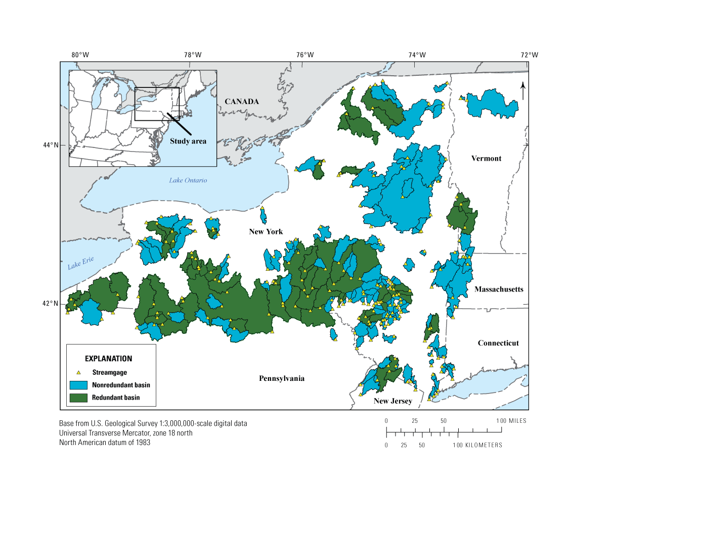
Map showing the delineated basins for the 213 unaltered streamgages used for this study in New York and adjacent States (U.S. Geological Survey, 2024b). Basins that were determined as nonredundant are shaded blue, and basins that were determined as redundant are shaded green (Stagnitta and Woda, 2025).
Basin Characteristics
A total of 224 basin characteristics were used as candidate predictor variables and were represented by variables that describe basin geometry, climatic conditions, land cover, soils and surficial geology, and other characteristics for each unaltered watershed (Koltun and Whitehead, 2002; Southard, 2013; Feaster and others, 2020).
Basin Geometry
Following basin delineation and determination of the total drainage area for each unaltered streamgage, additional basin characteristics related to the physical basin geometry were calculated from the delineated basins of all 213 unaltered streamgages. These additional basin characteristics were calculated and compiled by using the Zonal Statistics tool (in the Spatial Analyst toolbox in ArcGIS Pro, ver. 3.0), a geospatial tool commonly used to aggregate data by basin (for example, Goodman, and others, 2019; Lanping and others, 2021).
The basin elevation, slope, perimeter, relief, and several stream characteristics related to the longest flow path (including the slope and elevation) were determined by using a digital elevation model (DEM; U.S. Geological Survey, 2023a), the geometry tools in ArcGIS Pro (ver. 3.0), and custom ArcGIS software (Harvey and Eash, 1995; Stagnitta and Woda, 2025). The total stream length and stream density were determined by using the National Hydrography Dataset Plus (NHDPlus) version 2.1 dataset (Wieczorek and others, 2018; Stagnitta and Woda, 2025). In addition, the topographic wetness index, a measure that indicates how local topography affects both the direction and accumulation of overland flow, was calculated (Mattivi and others, 2019).
Climatic
Meteorological and climatic characteristics can influence both long- and short-term streamflow conditions. Climate related variations in low-streamflow conditions from year to year are primarily influenced by precipitation and temperature. Several temperature and precipitation variables were downloaded from the Parameter-Elevation Regressions on Independent Slopes Model (PRISM) Gridded Climate Dataset (PRISM Climate Group, 2014). The PRISM dataset was generated by using a digital elevation model to spatially interpolate long-term average precipitation and temperature datasets from 1981 to 2010 with a grid at a spatial resolution of 1 square kilometer for each cell. The temperature and precipitation datasets developed include the mean, minimum, and maximum across annual, monthly, and seasonal time intervals and were averaged within each unaltered basin by using Zonal Statistics (Stagnitta and Woda, 2025). In addition, the standard deviations for annual and monthly minimum and maximum values were averaged within each unaltered basin by using Zonal Statistics (Stagnitta and Woda, 2025).
The U.S. Drought Monitor compiles multiple drought indices and receives local input from cooperators to develop weekly maps of current drought conditions (U.S. Drought Monitor, 2023a). Data and information are compiled to develop spatial coverage maps, which include the severity of the current drought conditions ranked as follows: none, D0 (abnormally dry), D1 (moderate drought), D2 (severe drought), D3 (extreme drought), and D4 (exceptional drought). In addition, the U.S. Drought Monitor provides a historical dataset of weekly drought conditions from 2000 to the present.
Historical U.S. Drought Monitor conditions were obtained for the study area from January 2000 through December 2020. First, the weekly drought severity and coverage index was determined by multiplying the total area of drought (in square miles) by the current severity level (no drought, 0; D0, 1; D1, 2; D2, 3; and D3, 4) for each weekly dataset (U.S. Drought Monitor, 2023b). Second, the weekly shapefile dataset was converted to a raster dataset, and incremental values were assigned on the basis of the current drought conditions. For example, areas with no drought were assigned 0, whereas areas of D3 severity (extreme droughts) were assigned a value of 4. Finally, the sum of all weekly drought coverages was calculated across all years of data and the median was determined by using Zonal Statistics within each unaltered streamgage’s delineated basin (Stagnitta and Woda, 2025). This resulting index provides an estimate of the total amount of time and area (including severity) of drought in a basin, from 2000 to 2020.
Land Cover
The land cover types within a basin mediate the conveyance of rainfall runoff to streams and waterbodies. The National Land Cover Database (NLCD) 2021 includes several types of land cover classes derived from Landsat satellite imagery at a 30-meter spatial resolution (Dewitz, 2023). The land cover classes for each streamgage include the percentage of each basin covered by each of the following classes: open water, forest (deciduous, deciduous shrubland, evergreen, and mixed), wetland (woody and emergent), agriculture (fields, pasture, and agriculture), barren, developed (open space, low intensity, medium intensity, and high intensity), and shrublands. The land cover percentages were calculated using Zonal Statistics (ArcGIS Pro 3.0—Spatial Analyst toolbox; Stagnitta and Woda, 2025). A riparian area raster dataset was available from Abood and others, (2022) and was intersected with the NLCD forested and developed land cover classes (Stagnitta and Woda, 2025). Then, the percentage of each basin covered by the forested and developed riparian areas was determined by using Zonal Statistics. In addition, the national inventory of wetlands from the U.S. Fish and Wildlife Service was included as a separate land cover basin characteristic, and the percentage of each basin covered by wetlands, as designated by the U.S. Fish and Wildlife Service, was determined (U.S. Fish and Wildlife Service, 2023; Stagnitta and Woda, 2025).
Soils and Surficial Geology
The type of subsurface material within a basin influences the amount of groundwater storage available. Generally, basins with well-draining sand and gravel soils and surficial geological materials recharge groundwater storage in the spring, then discharge to streams during the dry summer months, and contribute to baseflow throughout the year (Randall and Freehafer, 2017). The types of surficial geologic materials included within the study include the following: alluvial, bedrock, bedrock/thin till, coarse, coarse/alluvial, colluvial, colluvial/weathered rock, fine, moraine, till, and wetland (selected from Shepps and others, 1959; Newell and others, 2000; Stone and others, 2002; Soller and others, 2009; Massachusetts Bureau of Geographic Information, 2022; Connecticut Department of Energy and Environmental Protection, 2023; New York State Museum, 2023; Vermont Agency of Natural Resources, 2023). Surficial geologic coverages are available at different resolutions on a State-by-State basis. National surficial coverage is available at a limited resolution (1:5,000,000 scale; Soller and others, 2009). To increase the resolution of this multi-State surficial geologic coverage, the highest resolution statewide coverages were joined together, and the national coverage was used to fill in areas with missing data. These datasets include the following:
-
• statewide (1:250,000) surficial geologic coverage for New York (New York State Museum, 2023),
-
• statewide (1:62,500) surficial geologic coverage for Vermont (Vermont Agency of Natural Resources, 2023),
-
• statewide (1:24,000) surficial geologic coverage for Massachusetts (Massachusetts Bureau of Geographic Information, 2022),
-
• statewide (1:24,000) surficial geologic coverage for Connecticut (Connecticut Department of Energy and Environmental Protection, 2023), and
-
• statewide (1:100,000) surficial geologic coverage for New Jersey (Newell and others, 2000; Stone and others, 2002; Stagnitta and Woda, 2025).
The information for soils is available from the Gridded Soil Survey Geographic Database (Soil Survey Staff, 2023). The soil survey database includes several types of related characteristics, such as hydrologic soil groups A, B, C, and D (zonal percent), slope gradient (zonal mean), root zone depth/storage (zonal mean), water table depth and storage (zonal mean), the presence of hydric soils (zonal percent), an erodibility factor (zonal percent), flood frequency (zonal percent), soil drainage class (zonal percent), nonirrigated capability classes 1–8 (zonal percent), soil loss tolerance factor classes 0–5 (zonal percent), and wind erodibility indices 0–250 (zonal percent; calculated with Spatial Analyst toolbox in ArcGIS Pro, ver. 3.0; Stagnitta and Woda, 2025). In addition, the percentages of the following soils classes were determined for each basin by using Zonal Statistics: coarse-silty, coarse-loamy, loamy, coarse-loamy-sandy-skeletal, sandy, sandy-skeletal, fine, fine-loamy-skeletal, fine-silty, and droughty soils (Stagnitta and Woda, 2025).
Other Characteristics
For each individual basin, the mean of each of the following additional basin characteristics was calculated by using Zonal Statistics:
-
• Subsurface contact time—estimated number of days when infiltrated water resides in the saturated subsurface zone of the basin before discharging into the stream (Wieczorek and others, 2018; Stagnitta and Woda, 2025);
-
• Horton overland flow—the average percentage of infiltration-excess overland flow in total streamflow, estimated by the watershed model TOPMODEL (Wolock, 2003b; Stagnitta and Woda, 2025); and
-
• Base flow index—interpolated base-flow index values, estimated at U.S. Geological Survey streamgages, used to develop 1-kilometer raster datasets nationwide (Wolock, 2003a; Stagnitta and Woda, 2025; base flow is the component of streamflow that can be attributed to groundwater discharge into streams).
Outlier Streamflow Data
Stagnitta and others (2024a) analyzed which streamgages were classified as altered and unaltered. For this study, 213 of the streamgages classified as unaltered in Stagnitta and others (2024a) were considered for use in developing the model to estimate 7Q10 and 30Q10 statistics for ungaged locations in New York. Streamgages classified as unaltered in Stagnitta and others (2024a) included streamgages that were determined to have “minor alterations”; that is, the streamflow at the streamgage showed limited alteration patterns from human activity upstream from the streamgage. The minor alterations of streamflow at 8 of the 213 study streamgages were determined to be too substantial for use in model development in this study. These eight streamgages were flagged as outliers on the basis of residual plots used during the initial development of the models, and remark comments were included on the NWIS web page for each streamgage (U.S. Geological Survey, 2024b).
The following Susquehanna River streamgages, which were classified as unaltered in Stagnitta and others (2024a), were later considered altered during development of the model because of slight alterations from upstream dams and reservoirs for flood control:
-
• 01531500 Susquehanna River at Towanda, Pennsylvania (drainage area 7,797 mi2),
-
• 01515000 Susquehanna River near Waverly, New York (drainage area 4,773 mi2),
-
• 01513831 Susquehanna River at Owego, N.Y. (drainage area 4,216 mi2),
-
• 01513500 Susquehanna River at Vestal, N.Y. (drainage area 3,941 mi2), and
-
• 01503000 Susquehanna River at Conklin, N.Y. (drainage area 2,232 mi2).
The following streamgages were also removed before modeling for reasons relating to flow alteration:
-
• 01326500 Hudson River at Spier Falls, N.Y. (drainage area 2,779 mi2)—Streamflow data were only available from 1912 to 1923, which predates the upstream reservoir built in 1930 at Sacandaga Lake,
-
• 04254500 Moose River at Mckeever, N.Y. (drainage area 363 mi2)—Streamflow has been altered by the upstream Fulton Chain Lakes in the Adirondack Mountains since about 1880, and
-
• 01512500 Chenango River near Chenango Forks, N.Y. (drainage area 1,483 mi2)—Streamflow is altered by upstream Whitney Point Lake and by slight diversions from upstream tributaries to the New York State Barge Canal.
Model Development
Recent literature has shown that machine learning methods can outperform more traditional modeling approaches such as multiple linear regression for estimating low-streamflow statistics in ungaged basins (Eng and others, 2017; Worland and others, 2018; Eng and Wolock, 2022; DelSanto and others, 2023). For example, Eng and Wolock (2022) compared the performance of multiple linear regression with three machine learning methods (random forest, cubist regression, and support vector regression) to evaluate the performance of each method for several streamflow statistics across the contiguous United States. The random forest regression model estimated the 7Q10 and 30Q10 low-streamflow statistics more accurately compared to other methods. DelSanto and others (2023) focused their study on the Northeast region of the United States and compared multiple methods of estimating 7Q10, including multiple linear regression, random forest, neural networks, and a generalized additive model. Overall, the random forest regression method more accurately predicted measured 7Q10 values compared to other methods across a range of small (less than 15 mi2), medium (15–70 mi2), and large (more than 70 mi2) basins in the Northeast.
The model development for this study used R code available from Zipper and others (2021) and followed a workflow similar to the one they used to evaluate stream intermittency across several stream metrics using a random forest regression model. The R packages tidymodels (Kuhn and Wickham, 2020), ranger (Wright and Ziegler, 2017), and partykit (Hothorn and Zeileis, 2015) were used to train, tune, and test random forest regression models to estimate 7Q10 and 30Q10 statistics for unaltered streamgages in the study area.
Figure 2 shows the modeling workflow used to evaluate the unaltered streamgages (that is, to identify redundant basins and outlier streamgages; after their removal, a total of 205 streamgages were available for development of the model), the 70/30 training/testing dataset split, and the modeling procedure to train, tune, and test the model. The following steps explains a more detailed description of the modeling workflow.
-
1. Log-transform the 7Q10 and 30Q10 dependent variables. Other transformations were explored such as dividing the low-streamflow statistics by the drainage area, but the log-transformation produced the most accurate output model results.
-
2. Randomly split 70 (143 streamgages) and 30 (62 streamgages) percent of the dataset into training and testing datasets (streamgages with basins flagged as redundant are not included in the testing dataset but can be included in the training dataset).
-
3. Train an initial random forest model by using a conditional random forest model to determine the most important predictor variables (described in more detail in the “Training—Variable Importance” section).
-
4. Train a second random forest model, in which the number of predictor variables is incrementally increased, starting with the most important variables (from step 3), and determine the models with the lowest mean square error (MSE) and coefficient of determination (R2; described in more detail in the “Training—Forward Feature Selection” section).
-
5. Use the results from step 4 to tune the model hyperparameters—mtry, the maximum number of predictor variables in an individual tree; ntree, the maximum number of trees; and min_n, the minimum number of nodes or observations in an individual tree—using a tenfold cross-validation procedure (the resampled training dataset does not include redundant basins, which is described in more detail in the “Model Tuning” section).
-
6. Test the tuned model with the 30-percent testing dataset and evaluate the performance of the model (described in more detail in the “Testing—Performance Metrics” section).
-
7. Bias-correct the modeled output data by using an empirical cumulative distribution function to match modeled output with the observed data (described in more detail in the “Bias Correction” section).
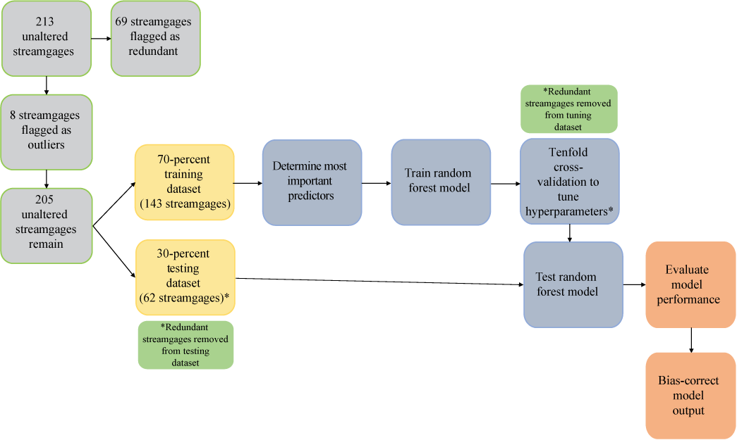
Diagram of the random forest regression model workflow used for this study (Stagnitta and Woda, 2025).
Training—Variable Importance
Random forest regression models do not generally lose performance when linearly correlated predictor variables are included in the models (Konapala and Mishra, 2020). A random forest regression model is developed using hundreds of decision trees: a randomly selected subset of predictor variables is used within each decision tree, and the best predictors from the random subset are selected at each split (Ishwaran and others, 2010). Groups of correlated predictor variables that are important for estimating the dependent variable are split into separate trees to diminish the influence of multicollinearity but can ultimately be included as potential predictor variables in the final model (Ishwaran and others, 2010).
The initial models developed to calculate the importance of each predictor variable use a conditional variable importance parameter to select variables with a significance level (p value) of 0.05 or lower (the hyperparameter mincriterion equal to 0.95). The conditional random forest regression model measures the “mean decrease in accuracy” and accounts for both the main and interactive effects among predictor variables (Strobl and others, 2008). Also, the ntree hyperparameter for the cforest function was set to a high number (1,750 trees) to ensure that the same predictor variables were output with different randomly sampled training and testing datasets. After the initial models to determine the conditional variable importance for all 224 basin characteristics were developed for this study, 188 and 192 basin characteristics remained for the 7Q10 and 30Q10 models, respectively (basin characteristics less than or equal to 0.05 significance level remained).
Training—Forward Feature Selection
The forward feature selection method is a common approach in machine learning to reduce the total number of predictor variables used for a model (Khalid and others, 2014; Meyer and others, 2018). Removing predictor variables that may not be relevant or are potentially redundant improves model accuracy (Khalid and others, 2014). Several search methods exist for identifying the optimal models, such as forward and backward feature selection and compound, weighted, and random feature selection (Khalid and others, 2014). The forward feature selection method incrementally increases the number of predictor variables in successive model runs, and predictor variables for the model with the lowest error are used for additional model tuning and testing.
The methods for this study includes the following three steps:
-
1. The output from the initial variable importance model was run to sort the predictor variables in order of importance.
-
2. The individual models were run while the number of predictor variables within each model was increased incrementally.
-
3. The model with the lowest MSE was determined.
The model with the lowest MSE is not always the best model to select, and models with fewer predictor variables are generally preferred (Helsel and others, 2020). Therefore, for this study, the total number of predictor variables within each model was considered. After forward feature selection models were developed and the total number of predictor variables was considered, the models with the 4th lowest (7Q10) and 5th lowest (30Q10) MSE, each of which had a total of 26 different predictor variables, were selected. A few models had lower MSE values (marginal improvements of log 0.01 ft3/s), but all these models had more than 30 predictor variables.
Model Tuning
The goal of model tuning is to provide an optimal tradeoff between underfitting and overfitting the dependent variable by tuning the model hyperparameters. A common approach to model tuning in machine learning applications is a k-fold cross-validation, in which the training dataset is randomly split into equally sized folds and each successive fold is held out as a validation dataset to tune the model (Meyer and others, 2018). In addition, Meyer and others (2018) determined that a “target-oriented” validation procedure, in which the spatial location of sites was considered, reduced overfitting and improved overall model accuracy. Sites that were in similar locations were separated from the random subset of the dataset for validating the models.
The random forest regression models included three hyperparameters to tune: the total number of predictor variables (mtry), the total number of trees (ntree), and the minimum number of observations or nodes within each tree (min_n). The models were tuned by a tenfold cross-validation procedure, in which 10 equally sized and randomly selected subsets of the 70-percent training dataset were held out individually to validate the model (redundant basins were removed from the 70-percent training dataset; a total of 80 streamgages remained). The cross-validation procedure allows for a grid search of the hyperparameters: mtry, which ranged from 1 to the maximum number of predictor variables determined from the forward feature selection for the 7Q10 and 30Q10 models (26 predictor variables for both 7Q10 and 30Q10), ntree, which ranged from 250 to 1,750, and min_n, which ranged from 3 to 25. The models with the lowest mean average error were selected, and the tuned hyperparameters were used for evaluating the performance of the models with the 30-percent testing dataset. The tuned 7Q10 model included a total of 8 predictor variables (mtry), 464 individual trees (ntree), and a minimum of 3 separate gaged observations within each tree (min_n). The tuned 30Q10 model included a total of 18 predictor variables (mtry), 464 individual trees (ntree), and a minimum of 3 separate gaged observations within each tree (min_n).
Testing—Performance Metrics
Performance metrics were used to evaluate how well each model fit to observed data from the testing dataset and included the following: the mean absolute error (MAE), the root mean square error (RMSE), the coefficient of determination (R2), and the Kling-Gupta efficiency (KGE). The KGE is similar to the Nash-Sutcliffe Efficiency in that the KGE accounts for bias, correlation, and variability as separate components (Gupta and others, 2009; Zipper and others, 2021). A KGE value more than or equal to −0.41 determines that a model is better than using the mean flow to estimate streamflows, and a perfect fit model has a KGE equal to 1 (Knoben and others, 2019 and Zipper and others, 2021).
There have been recent efforts to improve the interpretability of machine learning models, including the development of Shapley additive explanations (SHAP; Molnar, 2022). SHAP values are an estimation of Shapley values, a method derived from coalitional game theory, where features are “players,” and the prediction is the “payout” (Molnar, 2022). SHAP values are used to evaluate the explanatory power of the predictor variables on the individual predictions of the dependent variables (Lundberg and Lee, 2017). Several studies related to water resources have used SHAP values to aid in explaining the effects of predictor variables within a machine learning model related to water quality and quantity (Ransom and others, 2022; Madhushani and others, 2024). In this study, SHAP values were calculated and visualized by using the R packages fastshap (Greenwell, 2024) and shapvis (Mayer and Stando, 2024), respectively.
Results
The random forest regression models for finding the 7Q10 and 30Q10 statistics were evaluated by using a 30 percent testing dataset held out of the training and tuning procedures (Stagnitta and Woda, 2025). The streamflow values in the testing dataset ranged from 0.05 to 76.53 ft3/s for the 7Q10 model and from 0.08 to 91.99 ft3/s for the 30Q10 model. The ranges of the 7Q10, 30Q10, and basin characteristic values used for testing and training datasets for each model are shown in table 1.
Table 1.
The ranges of the ungaged lowest annual 7-day and 30-day average streamflow that occurs (on average) once every 10 years and the predictor basin characteristic values for the training and testing datasets used for developing models to estimate low-streamflow statistics at ungaged locations in New York (Stagnitta and Woda, 2025).[Basin characteristics are defined in the “Model Performance” section of this report. %, percent; 7Q10, the lowest annual 7-day average streamflow that occurs (on average) once every 10 years; 30Q10, the lowest annual 30-day average streamflow that occurs (on average) once every 10 years; ft3/s, cubic foot per second; NA, not applicable; mi2, square mile; mi, mile; ft/mi, foot per mile; in., inch; °F, degree Fahrenheit]
Model Performance
The 7Q10 and 30Q10 models yielded evenly distributed homoscedastic residuals and an adequate fit to the observed data (figs. 3 and 4). The overall performance results for the 7Q10 model (MAE equal to 3.214 ft3/s, RMSE equal to 5.686 ft3/s, R2 equal to 0.796, and KGE equal to 0.716) and the 30Q10 model (MAE equal to 3.677 ft3/s, RMSE equal to 6.133 ft3/s, R2 equal to 0.853, and KGE equal to 0.811) confirmed that the models accurately predicted 7Q10 and 30Q10 values, and the prediction accuracies were similar to those from the random forest models used for estimating low-streamflow statistics, which are described in the literature (Eng and Wolock, 2022; DelSanto and others, 2023).
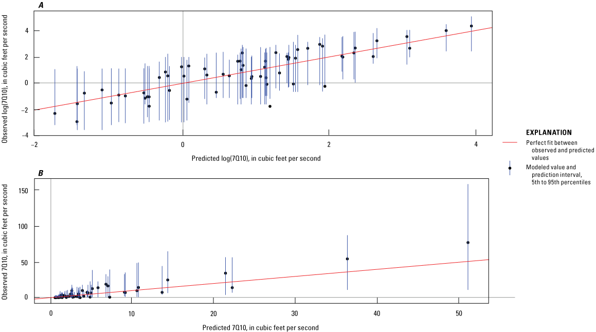
Graphs showing comparisons of estimated and observed 7Q10 in (A) log space and (B) real space. The red line represents a perfect fit between the observed and predicted values. The blue lines for each individual value represent the prediction interval between the 5th- and 95th-percentile modeled output values. 7Q10 is the lowest annual 7-day average streamflow that occurs (on average) once every 10 years.
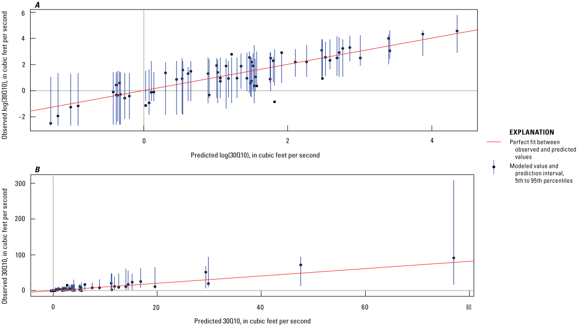
Graphs showing comparisons of predicted and observed 30Q10 in (A) and log space and (B) real space. The red line represents a perfect fit between the observed and predicted values. The blue lines for each individual value represent the prediction interval between the 5th- and 95th-percentile modeled output. 30Q10 is the lowest annual 30-day average streamflow that occurs (on average) once every 10 years.
The models tend to overpredict at lower 7Q10 (less than about 2.7 ft3/s) and 30Q10 (less than about 1 ft3/s) observed values in log space (figs. 3A and 4A). In addition, the models tend to underpredict at higher 7Q10 (greater than about 50 ft3/s) and 30Q10 (greater than about 75 ft3/s) observed values (figs. 3B and 4B). Prediction intervals were determined by using quantile random forest regression to calculate the 5th and 95th percentiles of individual predictions from the model (Meinshausen, 2006; Wright and Ziegler, 2017); these intervals indicate the uncertainty in the model-predicted streamflows.
Figures 5 and 6 show, for 7Q10 and 30Q10, the mean absolute SHAP value and the range of individual SHAP values for basin characteristics (in log space), and the figures include both the training and testing datasets for the top 8 and 18 most important predictor variables for the 7Q10 and 30Q10 models, respectively. SHAP values represent the explanatory power of each feature (basin characteristic) on an individual 7Q10 or 30Q10 value prediction (Molnar, 2022). Larger average SHAP values indicate a larger influence of the predictor variable on the estimate of the low-streamflow statistics.
Graph showing Shapley additive explanations (SHAP) values for the top 8 most important predictor variables for the 7Q10 model. The absolute mean SHAP value is the number displayed for each predictor variable, and the absolute mean values are shown in descending order. The SHAP values are calculated and displayed in the same units as the dependent variable (log-space 7Q10). Color-coded points represent the range of values for the predictor variable (cooler colors are lower values and warmer colors are higher values). The modeled outputs for both the training and testing datasets (205 streamgages) were used to generate this figure. Predictor variables are listed in table 1 and are defined in the “Model Performance” section of this report. 7Q10 is the lowest annual 7-day average streamflow that occurs (on average) once every 10 years.
Graph showing Shapley additive explanations (SHAP) values for the top 18 most important predictor variables for the 30Q10 model. The absolute mean SHAP value is the number displayed for each predictor variable, and the absolute mean values are shown in descending order. The SHAP values are calculated and displayed in the same units as the dependent variable (log-space 30Q10). Color-coded points represent the range of values for the predictor variable (cooler colors are lower values and warmer colors are higher values). The modeled output for both the training and testing datasets (205 streamgages) were used to generate this figure. Predictor variables are listed in table 1 and are defined in the “Model Performance” section of this report. 30Q10 is the lowest annual 30-day average streamflow that occurs (on average) once every 10 years.
The basin geometry characteristics Drainage_Area, Basin_Stream_Length, Basin_Perimeter, and Longest_Flow_Path were the most influential predictor variables for both the 7Q10 and 30Q10 models. These variables were well distributed from low to high SHAP values, indicating these variables are important for predicting both large and small 7Q10 and 30Q10 values.
Several additional basin characteristics differed in prediction influence for 7Q10 and 30Q10 models. Three basin characteristics were significant only for predicting 7Q10 values:
-
• Mean_Oct_Tmax—basinwide average of maximum October temperatures,
-
• Slope_LFP_Ratio—the ratio of the basin slope to the longest flow path, and
-
• Mean_Jun_Tmax—basinwide average of maximum June temperatures.
-
• SSURGO_Hydric_Class_Presence—the basinwide percentage of soils from the hydric class presence category (an indicator of wetland soils),
-
• STD_Apr_Tmin—the basinwide standard deviation of minimum April temperatures,
-
• Mean_Jun_Tmean—basinwide average of mean June temperatures,
-
• PS_Coarse_Loamy—basinwide percentage of soils classified as coarse-loamy,
-
• Mean_Mar_Precip—basinwide average of March precipitation,
-
• Mean_Apr_Tmean—basinwide average of mean April temperatures,
-
• STD_Oct_Tmax—the basinwide standard deviation of maximum October temperatures,
-
• STD_Aug_Tmax—basinwide standard deviation of maximum August temperatures,
-
• STD_Apr_Tmax—basinwide standard deviation of maximum April temperatures,
-
• Surficial_LF_Alluvial—basinwide percentage of the basin classified as alluvial surficial geologic materials,
-
• STD_Jun_Tmin—basinwide standard deviation of minimum June temperatures,
-
• STD_May_Tmin—basinwide standard deviation of minimum May temperatures, and
-
• Slope_LFP_Upper—the slope between the 0- and 50-percentile elevations along the longest flow path.
Bias Correction
Machine learning regression models, like many other related models, can systematically overestimate small values and underestimate large values (Belitz and Stackelberg, 2021). Belitz and Stackelberg (2021) evaluated six methods for correcting bias in predictions from machine learning regression models and determined that a simple empirical matching of the distributions of predicted values to observed values most accurately predicted hold-out datasets of all methods evaluated. Here, the training dataset was used to match the observed empirical distribution to the predicted values, and this distribution was then used to bias-correct predicted values from the testing dataset. Figures 7 and 8 show the cumulative distribution for the observed, modeled, and bias-corrected training and testing datasets. Figures 7A and 8A show that the modeled training dataset fits the observed distribution well before bias correction, whereas figures 7B and 8B show that when the models are used for testing with unseen data, the bias in predictions is pronounced. The testing dataset shows the bias in machine learning regression models to overestimate small values and underestimate large values, and the bias correction improves the predictions of these extreme values (figs. 7B and 8B). In addition, a bias correction in log space ensures that large 7Q10 or 30Q10 values do not dominate the distributions (Belitz and Stackelberg, 2021).
Graphs showing the cumulative distribution (in log space) for the observed, modeled, and bias-corrected 7Q10 values for both the (A) training and (B) testing datasets. 7Q10 is the lowest annual 7-day average streamflow that occurs (on average) once every 10 years.
Graphs showing the cumulative distribution (in log space) for the observed, modeled, and bias-corrected 30Q10 values for both the (A) training and (B) testing datasets. 30Q10 is the lowest annual 30-day average streamflow that occurs (on average) once every 10 years.
Discussion
Figures 3 and 4 show the 95-percent prediction interval for each modeled prediction of 7Q10 and 30Q10, and the potential ranges of predicted values were large (Stagnitta and Woda, 2025). The bias correction described in the previous section can help to reduce the error in predictions for new, unseen datasets, but there is still a level of uncertainty in the modeled output data. The percentages of observed values from the testing dataset outside the range of the prediction intervals were 4.8 (3 out of 62 streamgages) and 8.1 (5 out of 62 streamgages) for the 7Q10 and 30Q10 models, respectively.
The models were developed using a total of 205 unaltered or minimally altered streamgages. The models are not intended to be used in locations where there are potential human-induced effects on streamflow, such as withdrawals, dam operations, canal diversions, or high urbanization. If a user predicts a low-streamflow statistic at an ungaged location where there is a known flow alteration, the user should account for the potential effects of alteration.
Random forest models can accurately model low-streamflow statistics with smaller datasets (a few hundred observations), but model accuracy improves as the amount of observed data available to train the model increases. Biau (2012), found that model accuracy generally improved when at least 500 observations were included while training the model. As additional streamgages come online and newer data become available for model training, further updates and improvements to the models developed for this study may be warranted.
The models developed for this study were created to prioritize the prediction of 7Q10 and 30Q10 for ungaged locations across New York. These models were not developed to be used in basins with drainage areas outside the ranges in the training dataset (table 1). In addition, the models are not intended to be used to identify the physical drivers influencing low streamflow (correlated predictor variables in the final models diminish the usability of the models to describe the drivers). Because some variables in the final models were correlated, further study of the influence of predictor variables (described below) could improve understanding of the drivers of low-streamflow statistics in the study area.
The basin characteristics Drainage_Area, Basin_Stream_Length, Basin_Perimeter, and Longest_Flow_Path were the four most important predictor variables for the 7Q10 and 30Q10 models. These basin characteristics describe the physical topography and the overall length of streams within the basin and are the main physical drivers that determine the amount of runoff from precipitation that could be feasibly received within a network of streams. The models showed that larger values for these four predictor variables had larger low-streamflow statistics and that smaller variables had lower low-streamflow statistics.
In addition, the 7Q10 model included the slope between the most upstream and downstream points of the longest flow path divided by the mean basin slope (Slope_LFP_Ratio; determined by the intersection of basin polygon coverages and a digital elevation model). The 30Q10 model included the slope between the 0- and 50-percentile elevations of the longest flow path (Slope_LFP_Upper). The 7Q10 model showed that basins with a higher Slope_LFP_Ratio (basins in which the slope of the longest flow path and the mean basin slope were similar) had higher low-streamflow statistics. Generally, these were larger basins, in which the mean basin slope is less influenced by extreme elevations within the basin than basins with higher Slope_LFP_Ratio values (these were generally smaller basins). The Slope_LFP_Upper showed a similar pattern to the Slope_LFP_Ratio but to a much lesser extent: lower values of Slope_LFP_Upper corresponded to higher low-streamflow statistics.
Several basin characteristics related to temperature were included for the 7Q10 (Mean_Oct_Tmax and STD_Apr_Tmin) and 30Q10 (STD_Apr_Tmin, Mean_Jun_Tmean, Mean_Apr_Tmean, STD_Oct_Tmax, STD_Apr_Tmax, STD_Aug_Tmax, STD_May_Tmin, and STD_June_Tmin) models, respectively. The 7Q10 model showed that basins with higher maximum October temperatures tended to have lower 7Q10 values, indicating the influence of high temperatures in reducing streamflow during earlier fall months (September and October). The 30Q10 model showed a similar influence, to a lesser extent, of spring and early summer temperatures on streamflow. The 7Q10 and 30Q10 models showed that temperatures with a higher standard deviation or variability across the basin (on the basis of PRISM grid cells) of temperatures in spring, summer, and fall months for 7Q10 and 30Q10 models tended to have higher low-streamflow values. The higher variability temperature values occurred in basins that were largely forested and included both low and high elevations within the basins (Catskill and Adirondack Mountain regions). This may indicate basins with potentially more groundwater storage could provide more sustained low-streamflow values throughout the year. The 30Q10 model included the Mean_Mar_Precip, where lower values indicated lower low-streamflow statistics, which may indicate the importance of late winter or early spring precipitation in recharging groundwater-dominated basins.
In addition, basin characteristics related to soils and surficial geology were included with the 7Q10 model (SSURGO_HSGA) and 30Q10 model (SSURGO_Hydric_Class_Presence, SSURGO_HSGA, PS_Coarse_Loamy, Surficial_LF_Alluvial). The SSURGO_HSGA variable shows the percentage of the basin covered by hydrologic soil group A and is defined by well-draining soils. Basins with a low percentage of well-draining soils tended to have relatively low low-streamflow statistics. High SSURGO_HSGA percentages could be indicative of basins less able than others to infiltrate runoff to groundwater, and in such basins, groundwater would have less influence on streams during the seasonal low-streamflow period.
The 30Q10 model included more basin characteristics related to soils and surficial geology than the 7Q10 model. The 30Q10 low-streamflow statistics were calculated from a 30-day moving average, which is a longer period than the 7-day moving average used for the 7Q10 statistics. The soils and surficial geologic basin characteristics indicate a basin’s ability to store and mediate the flow of groundwater, which is likely more applicable to low-streamflow statistics calculated from longer moving average periods than from shorter periods. The percentage of the basin covered by the surficial coarse and loamy geologic soil class (PS_Coarse_Loamy) showed a pattern similar to that of the SSURGO_HSGA percentage but to a lesser degree: lower values corresponded to lower low-streamflow statistics. The percentage of the basin classified as “hydric” soils (SSURGO_Hydric_Class_Presence) is an indicator of wet soils and could also indicate the presence of wetlands; basins with higher percentages of hydric soils tended to have lower low-streamflow statistics than other basins. Generally, basins with wet soils and high percentages of wetlands store more water and could limit the amount of water available during the low-streamflow period. The percentage of the basin covered by the surficial geologic class of alluvial materials (Surficial_LF_Alluvial) showed a pattern similar to that of the SSURGO_Hydric_Class_Presence percentage but to a lesser degree: higher values of alluvium coverage corresponded to lower low-streamflow statistics.
The final models developed generally were well fit to the observed data, with an R2 of 0.796 for the 7Q10 model and an R2 of 0.853 for the 30Q10 model. The random forest regression model results are consistent with other studies across the Northeast and conterminous United States, which show that random forest regression models have higher prediction accuracies than models developed by linear regression methods (Eng and Wolock, 2022; DelSanto and others, 2023). DelSanto and others (2023) developed a random forest regression model for predicting 7Q10 across 106 streamgage locations from the Northeast, and they reported an R2 of 0.61 from a leave-one-out cross-validation procedure.
Additionally in this study, a bias-correction method was developed to remove bias by matching the distribution of predicted to observed values. The matched distribution can then be used to bias-correct new model results for ungaged locations. The bias correction will automatically be applied to output model results available in StreamStats.
StreamStats Web Application for Modeled Results in Ungaged Locations
The U.S. Geological Survey developed and maintains the interactive web application StreamStats (U.S. Geological Survey, 2024a). StreamStats provides functionality for users to delineate basins and obtain peak- and low-streamflow statistics for gaged and ungaged locations across the United States. The at-site 7Q10 and 30Q10 low-streamflow statistics calculated by Stagnitta and others (2024a) were the first low-streamflow statistics that were made available in StreamStats for New York. The interactive web application includes functionality to obtain predictions of 7Q10 and 30Q10 by using the models developed for this study in ungaged locations across the State. The tool includes functionality that allows users to click on a stream grid cell to delineate a basin and to then obtain basin characteristics and predictions for 7Q10 and 30Q10 statistics for ungaged locations. For more information about StreamStats and how to use the tool, refer to the help section of the web interface (U.S. Geological Survey, 2024a).
Summary
Low-streamflow statistics are often needed for applications related to permitting and drought monitoring in locations without available streamgages. The U.S. Geological Survey, in cooperation with the New York State Department of Environmental Conservation, used basin characteristics as predictor variables to develop random forest regression models to predict low-streamflow statistics at ungaged locations in New York, excluding Long Island but including hydrologically connected basins from bordering States. The models were trained, tuned, and tested to ensure that they performed well across the State. A redundancy analysis was performed for all basins with unaltered streamgages to flag those that were close in proximity and had similar drainage areas. The redundancy analysis flagged 69 gaged basins, which were removed from the testing dataset and cross-validation procedures to prevent data leaking from the training dataset to the testing dataset. In addition, 8 streamgages were flagged as outliers, and a total of 205 streamgages were available for model development.
Basin characteristics were developed across the following categories: basin geometry, climate, land cover, soils and surficial geology, and other characteristics. The basin characteristics were used as predictor variables in the model. The most important predictor variables were determined by developing a model to calculate initial conditional variable importance, and the total number of predictor variables was further reduced by using a forward feature selection method. The physical basin characteristics related to the drainage area, total stream length, the perimeter of the basin, and the longest flow path were the top predictor variables for the models of the lowest annual 7-day and 30-day average streamflow that occurs (on average) once every 10 years (7Q10 and 30Q10). Additional basin characteristics related to slope, temperature, precipitation, soils, and surficial geology were also important predictors for the models.
The models were trained to determine importance values of the predictor variables and to reduce the number of predictor variables for tuning by using a forward feature selection method. The models were tuned by using a tenfold cross-validation procedure to determine the optimal maximum number of predictor variables within each tree (mtry), the total number of decision trees within the random forest model (ntree), and the minimum number of observed data points within each tree (min_n). The models were evaluated by using the testing dataset held out from training, and results indicted well-fit generalized models, with coefficients of determination (R2) of 0.796 and 0.853 for the 7Q10 and 30Q10 models, respectively. The output model results for ungaged locations within the study area are available in StreamStats.
Acknowledgments
We would like to thank Rob Dudley and Cathy Chamberlin of the U.S. Geological Survey for their detailed reviews of this manuscript and data release. We would also like to thank Robin Glas and Chris Gazoorian of the U.S. Geological Survey, who developed the proposal for this work and were instrumental in securing funding to complete this project.
References Cited
Abood, S.A., Spencer, L., and Wieczorek, M., 2022, U.S. Forest Service national riparian areas base map for the conterminous United States in 2019: Forest Service Research Data Archive, accessed May 15, 2023, at https://doi.org/10.2737/RDS-2019-0030.
Belitz, K., and Stackelberg, P.E., 2021, Evaluation of six methods for correcting bias in estimates from ensemble tree machine learning regression models: Environmental Modelling & Software, v. 139, article 105006, 12 p., accessed April 23, 2024, at https://doi.org/10.1016/j.envsoft.2021.105006.
Biau, G., 2012, Analysis of a random forests model: Journal of Machine Learning Research, v. 13, no. 1, p. 1063–1095, accessed May 1, 2024, at https://www.jmlr.org/papers/volume13/biau12a/biau12a.pdf.
Connecticut Department of Energy and Environmental Protection, 2023, Surficial materials set: Connecticut Department of Energy and Environmental Protection dataset, accessed May 15, 2023, at https://deepmaps.ct.gov/maps/608054746f2d4577a5683c8f9d190d8f/about.
DelSanto, A., Bhuiyan, M.A.E., Andreadis, K.M., and Palmer, R.N., 2023, Low-flow (7-day, 10-year) classical statistical and improved machine learning estimation methodologies: Water, v. 15, no. 15, article 2813, 31 p., accessed March 13, 2024, at https://doi.org/10.3390/w15152813.
Dewitz, J., 2023, National Land Cover Database (NLCD) 2021 products: U.S. Geological Survey data release, accessed May 15, 2023, at https://doi.org/10.5066/P9JZ7AO3.
Eng, K., Grantham, T.E., Carlisle, D.M., and Wolock, D.M., 2017, Predictability and selection of hydrologic metrics in riverine ecohydrology: Freshwater Science, v. 36, no. 4, p. 915–926, accessed March 13, 2024, at https://doi.org/10.1086/694912.
Eng, K., Wolock, D.M., 2022, Evaluation of machine learning approaches for predicting streamflow metrics across the conterminous United States: U.S. Geological Survey Scientific Investigations Report 2022–5058, 27 p., accessed on March 13, 2024, at https://doi.org/10.3133/sir20225058.
Feaster, T.D., Kolb, K.R., Painter, J.A., and Clark, J.M., 2020, Methods for estimating selected low-flow frequency statistics and mean annual flow for ungaged locations on streams in Alabama (ver. 1.2, November 20, 2020): U.S. Geological Survey Scientific Investigations Report 2020–5099, 21 p., accessed on March 13, 2024, at https://doi.org/10.3133/sir20205099.
Feaster, T.D., and Lee, K.G., 2017, Low-flow frequency and flow-duration characteristics of selected streams in Alabama through March 2014: U.S. Geological Survey Scientific Investigations Report 2017–5083, 371 p., accessed March 13, 2024, at https://doi.org/10.3133/sir20175083.
Goodman, S., BenYishay, A., Lv, Z., and Runfola, D, 2019, GeoQuery—Integrating HPC systems and public web-based geospatial data tools: Computers and Geosciences, v. 122, p. 103–112, accessed June 11, 2024, at https://doi.org/10.1016/j.cageo.2018.10.009.
Greenwell, B., 2024, fastshap—Fast approximate shapley values (ver. 0.1.1): R software package, accessed April 18, 2024, at https://github.com/bgreenwell/fastshap.
Gupta, H.V., Kling, H., Yilmaz, K.K, and Martinez, G.F., 2009, Decomposition of the mean squared error and NSE performance criteria—Implications for improving hydrological modelling: Journal of Hydrology, v. 377, no. 1, p. 80–91, accessed April 15, 2024, at https://doi.org/10.1016/j.jhydrol.2009.08.003.
Harvey, C.A., and Eash, D.A., 1995, Description, instructions, and verification for Basinsoft, a computer program to quantify drainage-basin characteristics: U.S. Geological Survey Water-Resources Investigations Report 95–4287, 25 p., accessed June 15, 2023, at https://doi.org/10.3133/wri954287.
Helsel, D.R., Hirsch, R.M., Ryberg, K.R., Archfield, S.A., and Gilroy, E.J., 2020, Statistical methods in water resources: U.S. Geological Survey Techniques and Methods, book 4, chap. A3, 458 p., accessed September 2023 at https://doi.org/10.3133/tm4A3. [Supersedes USGS Techniques of Water-Resources Investigations, book 4, chap. A3, version 1.1.]
Hester, G., Carsell, K., and Ford, D., 2006, Benefits of USGS streamgaging program—Users and uses of USGS streamflow data: Denver, National Hydrologic Warning Council, prepared by David Ford Consulting Engineers, Inc., 17 p., accessed April 28, 2025, at https://www.hydrologicwarning.org/content.aspx?page_id=70&club_id=617218&item_id=3068&cat_id=8714.
Hothorn, T., and Zeileis, A., 2015, partykit—A modular toolkit for recursive partytioning in R: Journal of Machine Learning Research, v. 16, no. 118, p. 3905–3909, accessed April 3, 2024, at https://jmlr.org/papers/v16/hothorn15a.html.
Ishwaran, H., Kogalur, U.B., Gorodeski, E.Z., Minn, A.J., and Lauer, M.S., 2010, High-dimensional variable selection for survival data: Journal of the American Statistical Association, v. 105, no. 489, p. 205–217, accessed April 30, 2024, at https://doi.org/10.1198/jasa.2009.tm08622.
Khalid, S., Khalil, T., and Nasreen, S., 2014, A survey of feature selection and feature extraction techniques in machine learning, in Proceedings of 2014 Science and Information Conference, London, U.K., August 27–29, 2014: London, Science and Information Organization, p. 372–378, accessed April 5, 2024, at https://doi.org/10.1109/SAI.2014.6918213.
Knoben, W.J.M., Freer, J.E., and Woods, R.A., 2019, Technical note—Inherent benchmark or not? Comparing Nash-Sutcliffe and Kling-Gupta efficiency scores: Hydrology and Earth System Sciences, v. 23, no. 10, p. 4323–4331, accessed April 15, 2024, at https://hess.copernicus.org/articles/23/4323/2019/.
Koltun, G.F., and Whitehead, M.T., 2002, Techniques for estimating selected streamflow characteristics of rural, unregulated streams in Ohio: U.S. Geological Survey Water-Resources Investigations Report 02–4068, 50 p., accessed February 21, 2024, at https://doi.org/10.3133/wri024068.
Konapala, G., and Mishra, A., 2020, Quantifying climate and catchment control on hydrological drought in the continental United States: Water Resources Research, v. 56, no. 1, article e2018WR024620, 25 p., accessed April 30, 2024, at https://doi.org/10.1029/2018WR024620.
Kuhn, M., and Wickham, H., 2020, Tidymodels—A collection of packages for modeling and machine learning using tidyverse principles: R software packages, accessed April 3, 2024, at https://www.tidymodels.org.
Lanping T., Ke X., Yuanyuan C., Liye W., Qiushi Z., Weiwei Z., and Bangyong X., 2021, Which impacts more seriously on natural habitat loss and degradation? Cropland expansion or urban expansion?: Land Degradation & Development, v. 32, no. 2, p. 946–964, accessed June 11, 2024, at https://doi.org/10.1002/ldr.3768.
Lukasz, B.S., 2021, Methods for estimating low-flow frequency statistics, mean monthly and annual flow, and flow-duration curves for ungaged locations in Kansas: U.S. Geological Survey Scientific Investigations Report 2021–5100, 69 p., accessed February 21, 2024, at https://doi.org/10.3133/sir20215100.
Lundberg, S.M., and Lee, S.I., 2017, A unified approach to interpreting model predictions: Advances in neural information processing systems 30 [proceedings from Conference on Neural Information Processing Systems, 31st, Long Beach, Calif., Dec. 4-9, 2017], 10 p., accessed April 18, 2024, at https://proceedings.neurips.cc/paper_files/paper/2017/file/8a20a8621978632d76c43dfd28b67767-Paper.pdf.
Madhushani, C., Dananjaya, K., Ekanayake, I.U., Meddage, D.P.P., Kantamaneni, K., and Rathnayake, U., 2024, Modeling streamflow in non-gauged watersheds with sparse data considering physiographic, dynamic climate, and anthropogenic factors using explainable soft computing techniques: Journal of Hydrology, v. 631, article 130846, 19 p., accessed April 18, 2024, at https://doi.org/10.1016/j.jhydrol.2024.130846.
Massachusetts Bureau of Geographic Information, 2022, MassGIS Data—USGS 1:24,000 surficial geology: Massachusetts Bureau of Geographic Information digital datasets, accessed May 15, 2023, at https://www.mass.gov/info-details/massgis-data-usgs-124000-surficial-geology.
Mattivi, P., Franci, F., Lambertini, A., and Bitelli, G., 2019, TWI computation—A comparison of different open source GISs: Open Geospatial Data, Software and Standards, v. 4, article 6, 12 p., accessed June 11, 2024, at https://doi.org/10.1186/s40965-019-0066-y.
Mayer, M., and Stando, A., 2024, shapviz—SHAP visualizations (ver. 0.9.3): R software package, accessed April 18, 2024, at https://github.com/ModelOriented/shapviz.
Meinshausen, N., 2006, Quantile regression forests: Journal of Machine Learning Research, v. 7, no. 35, p. 983–999, accessed April 30, 2024, at https://jmlr.org/papers/v7/meinshausen06a.html.
Meyer, H., Reudenbach, C., Hengl, T., Katurji, M., and Nauss, T., 2018, Improving performance of spatio-temporal machine learning models using forward feature selection and target-oriented validation: Environmental Modelling & Software, v. 101, p. 1–9, accessed April 3, 2024, at https://doi.org/10.1016/j.envsoft.2017.12.001.
Molnar, C., 2022, Interpretable machine learning—A guide for making black box models explainable (2d ed.): [independently published], accessed April 18, 2024, at christophm.github.io/interpretable-ml-book/.
Newell, W.L., Powars, D.S., Owens, J.P., Stanford, S.D., and Stone, B.D., 2000, Surficial geologic map of central and southern New Jersey: U.S. Geological Survey Miscellaneous Investigations Series Map I–2540–D, 3 pls., 21-p. pamphlet, accessed May 15, 2023, at https://doi.org/10.3133/i2540D.
New York State Department of Environmental Conservation [NYSDEC], [1998], Technical and operational guidance series 1.3.1—Total maximum daily loads and water quality based effluent limits: New York State Department of Environmental Conservation Division of Water webpage, accessed January 7, 2025 at https://extapps.dec.ny.gov/docs/water_pdf/togs131.pdf.
New York State Museum, 2023, Surficial geology shape files: NYS GIS Clearinghouse digital datasets, accessed May 15, 2023, at https://www.nysm.nysed.gov/research-collections/geology/gis.
PRISM Climate Group, 2014, PRISM climate data: Oregon State University website, accessed January 16, 2022, at https://prism.oregonstate.edu.
R Core Team, 2023, R—A language and environment for statistical computing, version 4.3.2 (Eye Holes): R Foundation for Statistical Computing software release, accessed November 2023 at https://www.R-project.org/ and https://cran.r-project.org/src/base/R-4/.
Randall, A.D., 2010, Low flow of streams in the Susquehanna River basin of New York: U.S. Geological Survey Scientific Investigations Report 2010–5063, 57 p., accessed April 11, 2024, at https://pubs.usgs.gov/sir/2010/5063.
Randall, A.D., and Freehafer, D.A., 2017, Estimation of low-flow statistics at ungaged sites on streams in the Lower Hudson River Basin, New York, from data in geographic information systems: U.S. Geological Survey Scientific Investigations Report 2017–5019, 42 p., accessed April 11, 2024, at https://doi.org/10.3133/sir20175019.
Ransom, K. M., Nolan, B. T., Stackelberg, P. E., Belitz, K., and Fram, M. S., 2022, Machine learning predictions of nitrate in groundwater used for drinking supply in the conterminous United States: Science of the Total Environment, v. 807, pt. 3, article 151065, 11 p., accessed April 18, 2024, at https://doi.org/10.1016/j.scitotenv.2021.151065.
Shepps, V.C., White, G.W., Droste, J.B., and Sitler, R.F., 1959, Glacial geology of northwestern Pennsylvania: Pennsylvania Geological Survey Bulletin G–32, digital data, scale 1:125,000, accessed May 15, 2023, at https://www.pasda.psu.edu/uci/DataSummary.aspx?dataset=1452.
Smakhtin, V.U., 2001, Low flow hydrology—A review: Journal of Hydrology, v. 240, nos. 3–10, p. 147–186, accessed February 21, 2024, at https://doi.org/10.1016/S0022-1694(00)00340-1.
Soller, D.R., Reheis, M.C., Garrity, C.P., and Van Sistine, D.R., 2009, Map database for surficial materials in the conterminous United States: U.S. Geological Survey Data Series 425, digital data, scale 1:5,000,000, accessed May 15, 2023, at https://pubs.usgs.gov/ds/425/.
Soil Survey Staff, 2023, Gridded Soil Survey Geographic Database for the conterminous United States [June 2023 release]: U.S. Department of Agriculture, Natural Resources Conservation Service, accessed June 12, 2023, at https://gdg.sc.egov.usda.gov/.
Southard, R.E., 2013, Computed statistics at streamgages, and methods for estimating low-flow frequency statistics and development of regional regression equations for estimating low-flow frequency statistics at ungaged location in Missouri: U.S. Geological Survey Scientific Investigations Report 2013–5090, 28 p., accessed August 15, 2024 at https://doi.org/10.3133/sir20135090.
Stagnitta, T.J., Graziano, A.P., Woda, J.C., Glas, R.L., and Gazoorian, C.L., 2024a, Low-flow statistics for selected streams in New York, excluding Long Island: U.S. Geological Survey Scientific Investigations Report 2024–5055, 39 p., accessed August 15, 2024, at https://doi.org/10.3133/sir20245055.
Stagnitta, T.J., Graziano, A.P., Woda, J.C., Glas, R.L., and Gazoorian, C.L., 2024b, Low-flow statistics for New York State, excluding Long Island, computed through March 2022: U.S. Geological Survey data release, accessed August 15, 2024, at https://doi.org/10.5066/P9NOM6FR.
Stagnitta, T.J., and Woda, J.C., 2025, Random forest regression model archive for estimating low-streamflow statistics at ungaged locations in New York, excluding Long Island: U.S. Geological Survey data release, https://doi.org/10.5066/P146MTRS.
Stone, B.D, Stanford, S.D., and Witte, R.W., 2002, Surficial geologic map of northern New Jersey: U.S. Geological Survey Miscellaneous Investigations Series Map I–2540–C, 3 sheets, scale 1:100,000, 41-p. pamphlet, accessed May 15, 2023, at https://doi.org/10.3133/i2540C.
Strobl, C., Boulesteix, A.-L., Kneib, T., Augustin, T., and Zeileis, A., 2008, Conditional variable importance for random forests: BMC Bioinformatics, v. 9, no. 1, article 307, 11 p., accessed May 1, 2024, at https://doi.org/10.1186/1471-2105-9-307.
U.S. Drought Monitor, 2023a, Data tables—Percent area in U.S. drought monitor categories [New York]: National Drought Mitigation Center dataset, accessed August 14, 2023, at https://droughtmonitor.unl.edu/DmData/DataTables.aspx.
U.S. Drought Monitor, 2023b, Drought severity and coverage index: National Drought Mitigation Center web page, accessed August 14, 2023, at https://droughtmonitor.unl.edu/About/AbouttheData/DSCI.aspx.
U.S. Fish and Wildlife Service, 2023, U.S. Fish and Wildlife Service National Wetlands Inventory: U.S. Fish and Wildlife Service digital data, accessed May 15, 2023, at https://www.fws.gov/wetlands/Data/Mapper.html.
U.S. Geological Survey, 2023a, 1/3rd arc-second digital elevation models (DEMs)—USGS National Map 3DEP downloadable data collection: U.S. Geological Survey dataset, accessed June 15, 2023, at https://www.sciencebase.gov/catalog/item/4f70aa9fe4b058caae3f8de5.
U.S. Geological Survey, 2023b, StreamStats batch processor (ver. 1.0.0, October 20, 2023): U.S. Geological Survey StreamStats database tool, accessed 2023, at https://streamstats.usgs.gov/ss/?BP=submitBatch.
U.S. Geological Survey, 2024a, StreamStats (ver. 4.19.4, February 8, 2024): U.S. Geological Survey map viewer, accessed April 15, 2024, at https://streamstats.usgs.gov/ss/.
U.S. Geological Survey, 2024b, USGS water data for the Nation: U.S. Geological Survey National Water Information System database, accessed June 3, 2024, at https://doi.org/10.5066/F7P55KJN.
Veilleux, A.G., and Wagner, D.M., 2021, Methods for estimating regional skewness of annual peak flows in parts of eastern New York and Pennsylvania, based on data through water year 2013: U.S. Geological Survey Scientific Investigations Report 2021–5015, 38 p., accessed August 15, 2024 at https://doi.org/10.3133/sir20215015.
Vermont Agency of Natural Resources, 2023, Surficial geologic map of Vermont, 1970—Units: Vermont Open Geodata Portal website, accessed May 15, 2023, at https://geodata.vermont.gov/datasets/VTANR:surficial-geologic-map-of-vermont-1970-units/about.
Wieczorek, M.E., Jackson, S.E., and Schwarz, G.E., 2018, Select attributes for NHDPlus version 2.1 reach catchments and modified network routed upstream watersheds for the conterminous United States (ver. 4.0, August 2023): U.S. Geological Survey data release, accessed August 8, 2023 at https://doi.org/10.5066/F7765D7V.
Wolock, D.M., 2003a, Base-flow index grid for the conterminous United States: U.S. Geological Survey data release, accessed August 8, 2023 at https://doi.org/10.5066/P9MCTH3J.
Wolock, D.M., 2003b, Infiltration-excess overland flow estimated by TOPMODEL for the conterminous United States: U.S. Geological Survey data release, accessed August 8, 2023 at https://doi.org/10.5066/P9QNTGCQ.
Worland, S.C., Farmer, W.H., and Kiang, J.E., 2018, Improving predictions of hydrological low-flow indices in ungaged basins using machine learning: Environmental Modelling & Software, v. 101, p. 169–182, accessed March 13, 2024, at https://doi.org/10.1016/j.envsoft.2017.12.021.
Wright, M.N., and Ziegler, A., 2017, ranger—A fast implementation of random forests for high dimensional data in C++ and R: Journal of Statistical Software, v. 77, no. 1, p. 1–17, accessed April 3, 2024, at https://doi.org/10.18637/jss.v077.i01.
Zipper, S.C., Hammond, J.C., Shanafield, M., Zimmer, M., Datry, T., Jones, C.N., Kaiser, K.E., Godsey, S.E., Burrows, R.M., Blaszczak, J.R., Busch, M.H., Price, A.N., Boersma, K.S., Ward, A.S., Costigan, K., Allen, G.H., Krabbenhoft, C.A., Dodds, W.K., Mims, M.C., Olden, J.D., Kampf, S.K., Burgin, A.J., and Allen, D.C., 2021, Pervasive changes in stream intermittency across the United States: Environmental Research Letters, v. 16, no. 8, article 084033, 16 p, accessed March 19, 2023, at https://doi.org/10.1088/1748-9326/ac14ec.
Conversion Factors
Abbreviations
30Q10
the lowest annual 30-day average streamflow that occurs (on average) once every 10 years
7Q10
the lowest annual 7-day average streamflow that occurs (on average) once every 10 years
D0
abnormally dry
D1
moderate drought
D2
severe drought
D3
extreme drought)
D4
exceptional drought
DAR
drainage area ratio
KGE
Kling-Gupta efficiency
MAE
mean absolute error
MSE
mean square error
NLCD
National Land Cover Database
NWIS
National Water Information System
NYSDEC
New York State Department of Environmental Conservation
PRISM
Parameter-Elevation Regressions on Independent Slopes Model
R2
coefficient of determination
RMSE
root mean square error
SD
standardized distance
SHAP
Shapley additive explanations
Director, New York Water Science Center
U.S. Geological Survey
425 Jordan Road
Troy, NY 12180–8349
dc_ny@usgs.gov
or visit our website at
Disclaimers
Any use of trade, firm, or product names is for descriptive purposes only and does not imply endorsement by the U.S. Government.
Although this information product, for the most part, is in the public domain, it also may contain copyrighted materials as noted in the text. Permission to reproduce copyrighted items must be secured from the copyright owner.
Suggested Citation
Stagnitta, T.J., Woda, J.C., and Graziano, A.P., 2025, Random forest regression models for estimating low-streamflow statistics at ungaged locations in New York, excluding Long Island: U.S. Geological Survey Scientific Investigations Report 2025–5060, 23 p., https://doi.org/10.3133/sir20255060.
ISSN: 2328-0328 (online)
Study Area
| Publication type | Report |
|---|---|
| Publication Subtype | USGS Numbered Series |
| Title | Random forest regression models for estimating low-streamflow statistics at ungaged locations in New York, excluding Long Island |
| Series title | Scientific Investigations Report |
| Series number | 2025-5060 |
| DOI | 10.3133/sir20255060 |
| Publication Date | August 01, 2025 |
| Year Published | 2025 |
| Language | English |
| Publisher | U.S. Geological Survey |
| Publisher location | Reston, VA |
| Contributing office(s) | New York Water Science Center |
| Description | Report: v, 23 p.; 2 Data Releases |
| Country | United States |
| State | New York |
| Other Geospatial | New York excluding Long Island |
| Online Only (Y/N) | Y |
| Additional Online Files (Y/N) | N |