

Methods for Estimating Selected Low-Flow Statistics at Gaged and Ungaged Stream Sites in Massachusetts
Links
- Document: Report (7.49 MB pdf) , HTML , XML
- Data Releases:
- USGS data release - Low-flow statistic equations and supplementary data for Massachusetts
- USGS data release - MODPATH6 datasets using MODFLOW and SEAWAT input for development of groundwater contributing areas for estimating low-flow statistics for the Plymouth-Carver aquifer area and Cape Cod, Massachusetts
- USGS data release - Low-flow statistic equations and supplemental data for the Plymouth-Carver Kingston-Duxbury aquifer area in southeastern Massachusetts and Cape Cod
- Download citation as: RIS | Dublin Core
Acknowledgments
The authors thank Viki Zoltay (Massachusetts Department of Conversation and Recreation, Office of Water Resources), Julie Butler (Massachusetts Department of Environmental Protection), and Kate Bentsen (Massachusetts Division of Ecological Restoration) for providing their expertise and input for this study.
Thanks are extended to Carl Carlson, Timothy McCobb, Donald Walter, and John Masterson of the U.S. Geological Survey (USGS) for expertise on groundwater models and modeling techniques for the Plymouth-Carver-Kingston-Duxbury aquifer system in southeastern Massachusetts and on Cape Cod. Additionally, thanks to Caroline Mazo, Luke Sturtevant, Kristina Hyslop, and Alex Butcher of the USGS for providing their geographic information system expertise to this study.
Abstract
The U.S. Geological Survey, in cooperation with the Massachusetts Department of Conservation and Recreation, Office of Water Resources, computed selected at-site streamflow statistics at U.S. Geological Survey streamgages in and near Massachusetts and developed regional regression equations for estimating selected streamflows at ungaged stream sites in Massachusetts. Two sets of regional regression equations were developed: (1) the “mainland” equations, for mainland Massachusetts excluding the area covered by the second set, and (2) the “southeastern” equations, for the Plymouth-Carver-Kingston-Duxbury aquifer area in southeastern Massachusetts and for Cape Cod. The regression equations and at-site statistics may be used by Federal, State, and local water managers in addressing water-resources issues relevant in Massachusetts.
Regional regression analyses for the mainland equations were developed to estimate the following 27 streamflow statistics: 99-, 98-, 95-, 90-, 85-, 80-, 75-, 70-, 60-, and 50-percent flow durations; monthly June, July, August, and September 90- and 50-percent flow durations; February, June, and August median of the monthly means; harmonic mean; and medians of the following annual low-flow frequency statistics: 7-day; 7-day, 2-year; 7-day, 10-year; 30-day, 2-year; and 30-day, 10-year. The analyses used 81 streamgages with minimal to no regulations in and near Massachusetts. The regression analyses determined that four basin characteristics—drainage area, combined hydrologic soils A and B, streamflow variability index, and annual mean temperature—were the only significant explanatory variables for the different mainland equations.
Regional regression equations were developed for the Plymouth-Carver-Kingston-Duxbury aquifer area in southeastern Massachusetts and Cape Cod, because surface-water drainage areas and groundwater contributing areas do not always coincide in this area of the State. The regression analyses to estimate 10 flow durations from the 99th to 50th percentiles used 18 streamflow sites with some occasional minor regulations—because there are few unregulated streams in southeastern Massachusetts. The analyses determined that groundwater contributing area and storage (combined water bodies and wetlands) were the only significant explanatory variables in the southeastern equations.
Introduction
Flow statistics for streams are crucial for water-resources planning, management, and permitting to allocate adequate water for consumptive use, water-quality standards, recreation, and aquatic habitat. For example, the minimum 7-day-average flow that has a probability of occurring once every 10 years (7Q10) is a streamflow statistic used as a hydrologically-based design flow for water-quality standards and toxic wasteload allocation studies relating to chronic effects on aquatic life (U.S. Environmental Protection Agency, 1986). Information on streamflow statistics is critical for water-resource managers, especially during drought periods. In Massachusetts, drought periods have occurred during 1879–83 and 1908–12 (Kinnison, 1931); 1929–32, 1939–44, 1961–69, and 1980–83 (Walker and Lautzenheiser, 1991); and 1985–88, 1995, 1998–1999, 2001–03, 2007–08, 2010, and 2016–17 (Massachusetts Executive Office of Energy and Environmental Affairs and Massachusetts Emergency Management Agency, 2023). In 2020 and 2022, Massachusetts also experienced drought conditions across parts of the State (Massachusetts Water Resources Commission, 2024). Most of these drought periods correspond to intervals when the annual mean streamflow was below the mean annual streamflow of 75 cubic feet per second (ft3/s) at Wading River at Norton (01109000) in southeastern Massachusetts and of 200 ft3/s at West Branch Westfield River at Huntington (01181000) in western Massachusetts for their periods of record (figs. 1 and 2). Although these streamgages have minimal to no regulations, the major drought and wet periods during water years 1924–2023 are reflected in the mean annual streamflows.
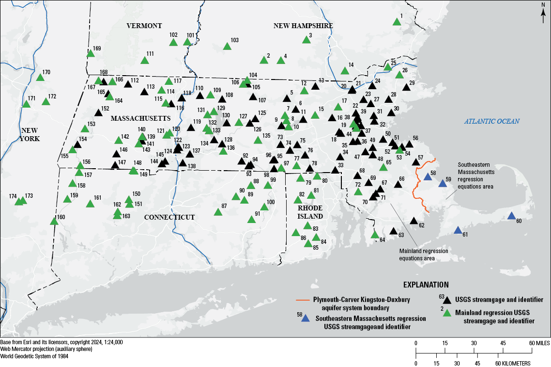
Locations of U.S. Geological Survey (USGS) streamgages in and near Massachusetts for which at-site low-flow statistics were computed. Streamgages used in the mainland Massachusetts low-flow regional regression equations are green triangles and in the southeastern Massachusetts equations are blue triangles. Streamgages described in table 1.
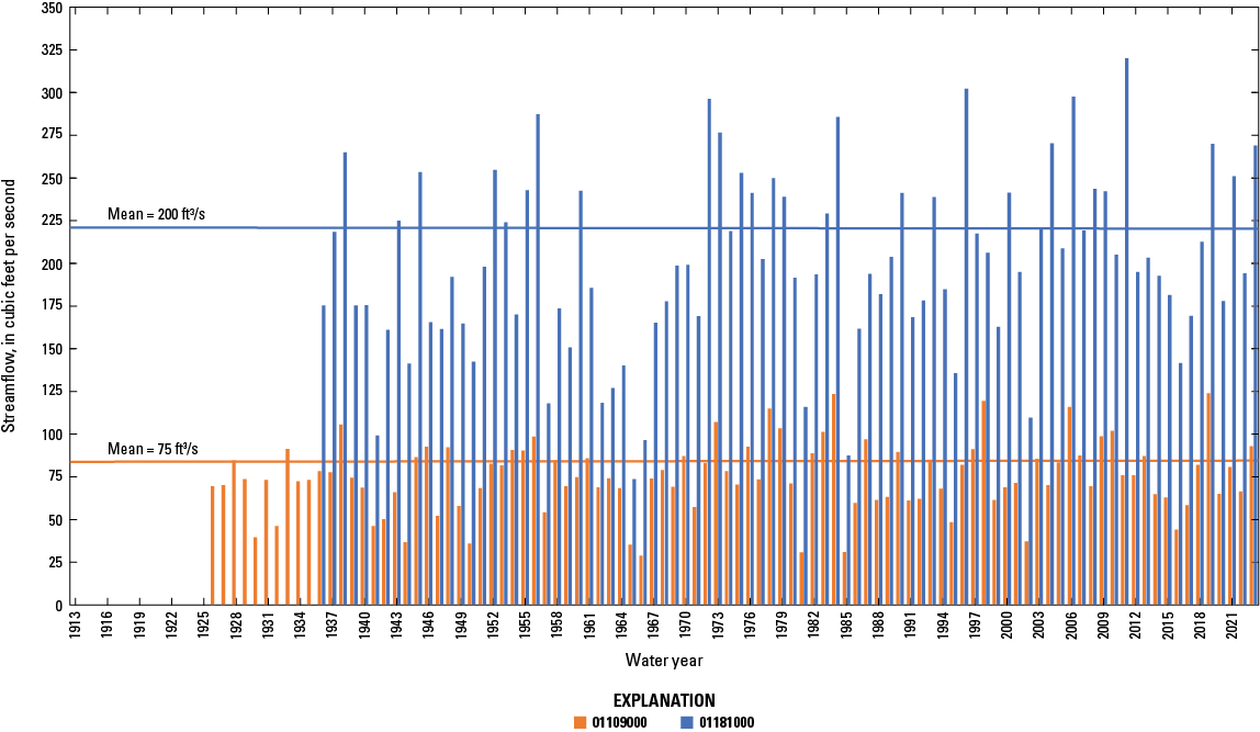
Mean annual streamflows at the U.S. Geological Survey streamgages Wading River at Norton, Massachusetts (01109000; map number 69), and West Branch Westfield River at Huntington, Mass. (01181000; map number 143), for water years 1926–2022 and 1936–2022, respectively. Streamgages shown in figure 1 and described in table 1. ft3/s, cubic foot per second.
Massachusetts streamflow standards have been a critical topic since the 1980s. In 1986, the Massachusetts Department of Environmental Protection’s (MassDEP) Water Management Act (WMA) Program began to regulate the amount of water withdrawn from groundwater and surface-water resources (Massachusetts Department of Environmental Protection, 2023). The WMA allocates adequate supplies for current and future needs, while taking into account the potential effects on aquatic habitats. Some permits for water-supply withdrawals in Massachusetts are linked to selected streamflow or groundwater level statistics of selected U.S. Geological Survey (USGS) streamgages or observation wells, respectively (Duane LeVangie, Massachusetts Department of Environmental Protection, written commun., 2022; Massachusetts Department of Environmental Protection, 2024b).
In 1999, the Massachusetts Water Resources Commission directed an interagency committee to define a “stressed basin,” which includes water quantity, quality, and habitat factors (Massachusetts Water Resources Commission, 2023). In 2003, the Massachusetts Water Resources Commission began a study to determine “index streamflows” (Massachusetts Department of Conservation and Recreation, Office of Water Resources, 2008). This study included determining streamflow statistics by using three different approaches (target hydrograph, aquatic base flow, and indicators of hydrologic alteration) at the index gages (minimal to no regulations) in and near Massachusetts.
The U.S. Environmental Protection Agency (EPA) and MassDEP regulate wastewater discharges in Massachusetts through the National Pollutant Discharge Elimination System (NPDES). NPDES permits are based on selected streamflow statistics of the receiving streams, such as the 7Q10, harmonic mean, or 30Q10 (30-day, 10-yr) flow (U.S. Environmental Protection Agency, 1986). Regulatory determination of the perennial and intermittent status of streams also uses streamflow statistics. Streams shown as intermittent on a USGS topographic map with drainage areas between 0.5 and 1 square mile (mi2) are determined to be perennial if the 99-percent flow duration is equal to or greater than 0.01 ft3/s (Massachusetts Department of Environmental Protection, 2024a). Finally, the August median flow is an important statistical measure for fisheries and often is used for the summer maintenance of aquatic habitat in New England streams (U.S. Fish and Wildlife Service, 1981).
This study was completed between 2019–24 by the USGS in cooperation with the Massachusetts Department of Conservation and Recreation, Office of Water Resources. The study provides regression equations for estimating selected streamflow statistics for ungaged stream sites and at-site streamflow statistics for many streamgages in and near Massachusetts. Streamflow statistics can inform planning, management, and permitting decisions related to providing adequate water for consumptive use, water-quality standards, recreation, and aquatic habitat in Massachusetts.
Purpose and Scope
This report describes regression equations developed for estimating selected statistics for streamflows in Massachusetts from basin characteristics (hydrography, elevation, physical, land-use, soil, surficial geology, and climate). The selected streamflow statistics estimated with the regression equations are for near-natural flow conditions (minimal to no regulations). Regression equations were developed for selected streamflow statistics, including selected annual and monthly flow durations; selected monthly median flows; selected 7- and 30-day low-flow frequencies; and other statistics, such as the harmonic mean, for the mainland area of Massachusetts (fig. 1) (hereafter referred to as the “mainland” equations). Selected streamflow statistics are also provided for streamgages with regulations and streamgages with minimal to no regulations in and near Massachusetts. These statistics include the ones estimated for the regression equations and other selected annual flow durations for higher streamflows, monthly flow durations, and median of the monthly means streamflows. The streamflow statistics, basin characteristics, streamflow variability index, and regression analyses for the mainland equations are provided in a USGS data release (Bent and others, 2025).
A separate set of regression equations were developed that only estimate annual flow durations between the 50- and 99-percentiles for the Plymouth-Carver-Kingston-Duxbury aquifer system in southeastern Massachusetts and Cape Cod (fig. 1; hereafter referred to as the “southeastern” equations). Additionally, similar streamflow statistics, for which equations were not developed, are also provided for the southeastern area. The streamflow statistics, basin characteristics (aquifer, elevation, physical, land-use, soil, surficial geology, and climate), regression analyses, and other information for the southeastern equations are provided in a separate USGS data release (Carlson, 2025; Sturtevant and others, 2025).
An evaluation of the accuracies of both the mainland and southeastern equations and the limitations for their use is provided, as are considerations for further studies. Discussion about the USGS StreamStats web-based application is also provide in the report.
Previous Studies
Fennessey and Vogel (1990), Vogel and Kroll (1990), Ries (1990), Risley (1994), Ries (1994a, b, 1997, 1999), Ries and Friesz (2000), Ries and others (2000), and Archfield and others (2010) provided estimated streamflow statistics and regression equations for various flow durations such as the 7-day, 2-year low-flow frequency (7Q2) and 7Q10 in Massachusetts. These studies have included equations for low-flow frequencies and low-flow durations. Explanatory variables for the low-flow equations in these studies have included drainage area, area of stratified-drift deposits per unit of total stream length, mean basin slope, basin relief (maximum minus minimum basin elevation), average annual precipitation, open water, sand and gravel deposits, average maximum monthly temperature, X- and Y-location of basin outlet, X- and Y-location of basin centroid, and region of the State.
Wandle and Randall (1994) developed regression equations for estimating low-flow frequencies, 7Q2 and 7Q10, for high- and low-relief regions of central New England. Explanatory variables for the equations included drainage area, surficial geology, area of swamps and lakes, mean basin elevation, mean channel length, and mean annual runoff. Wandle (1983, 1987) previously developed low-flow-frequency and flow-duration equations for Massachusetts and New England, respectively. Ries (1990) developed regression equations to estimate monthly and mean annual runoff from major drainage areas in Massachusetts and Rhode Island draining to Narragansett Bay. Explanatory variables for the equations included area of till, area of stratified-drift deposits and storage (water bodies and swamps), and area of urban land. Armstrong and others (2008) provided regression equations for estimating median monthly streamflows in Massachusetts. DelSanto and others (2023) developed equations for estimating the 7Q10 for the northeastern United States (included Massachusetts streamgages) using linear regression and machine learning estimation methodologies: random forest decision trees, neural networks, and generalized additive models. Their equations included the minimum 30-day cumulative precipitation and average 30-day high temperature as well as drainage area, slope, mean elevation, wetlands area, and forest area. Bent and Archfield (2002) and Bent and Steeves (2006) provided logistic regression equations for estimating the probability of a stream flowing perennially in Massachusetts.
Regression equations for estimating selected low-flow statistics have been published in Connecticut, Rhode Island, New Hampshire, and New York studies over the last 20 years. Low-flow equations have not, currently (2025), been developed for Vermont. Ahearn and others (2006) and Ahearn (2008, 2010) and provided estimated streamflow statistics and regression equations for various flow durations, 7Q2, 7Q10, and seasonal flows based on aquatic habitat needs in Connecticut. Kliever (1996) estimated the 99-, 98-, 97-, 95-, 90-, 85-, 80-, 70-, 60-, 50-percent flow durations, 7Q10, and mean monthly streamflows for August, February, April, and May for 16 partial-record stations in northern Rhode Island. Cervione and others (1993) calculated the 99-, 98-, 95-, 90-, and 80- percent flow durations for 25 partial-record stations in southern Rhode Island. Cervione and others (1993) also presented a regression equation to estimate the 7Q10 for selected streams in Rhode Island. Bent and others (2014) provided low-flow equations for the 99- to 1-percent flow duration and the 7Q2 and 7Q10 in Rhode Island. Flynn (2003a, b) developed low-flow equations to estimate seasonal (winter, spring, summer, and fall) and annual 98-, 95-, 90-, 80-, 70-, and 60-percent flow durations and the 7Q2 and 7Q10 in New Hampshire. Randall and Freehafer (2017) developed low-flow equations for the lower Hudson River Basin, New York (area adjacent to Massachusetts and Connecticut), for the 7Q2 and 7Q10.
Description of Study Area
Low flows are greatly affected by the geography, climate, and surficial geology upstream from the measurement location. Massachusetts encompasses 8,093 mi2 in the northeastern United States (fig. 1). Elevations range from sea level in coastal areas to about 3,500 feet (ft) above sea level (referenced to the North American Vertical Datum of 1988 [NAVD 88]) in the northwest. Elevations generally increase from eastern to western Massachusetts. The climate in Massachusetts is humid, with average annual precipitation ranging from about 40 to 45 inches (in.) in eastern Massachusetts to about 40 to 50 in. in western Massachusetts, where higher elevations may cause orographic effects. Average annual temperature is about 50 degrees Fahrenheit (°F) in eastern Massachusetts and about 45 °F in western Massachusetts (Bent and Waite, 2013). About half of the annual precipitation is returned to the atmosphere through evaporation and plant transpiration, with the remainder becoming groundwater recharge or stream runoff (Bent and Waite, 2013).
Surficial deposits that overlie bedrock in most of Massachusetts were deposited mainly during the last glacial period but can include areas of recent floodplain alluvium deposits along rivers and streams (Bent and Waite, 2013). In this report, these surficial deposits are classified as either till (which includes till, till with bedrock outcrops, sandy till over sand, and end-moraine deposits) or stratified deposits (which include sand and gravel, coarse sand, floodplain alluvium deposits, and fine-grained sand). Till (also known as ground moraine) is an unsorted, unstratified mixture of clay, silt, sand, gravel, cobbles, and boulders, typically deposited by glaciers on top of bedrock throughout much of the State. Till is primarily found in upland areas but can also be found at depth in river valleys. Stratified deposits include sorted and layered glaciofluvial and glaciolacustrine deposits. Glaciofluvial deposits are material of all grain sizes (clay, silt, sand, gravel, and cobbles) deposited by glacial meltwater streams in outwash plains and river valleys. Glaciolacustrine deposits generally consist of clay, silt, and fine sand deposited in temporary lakes that formed after the retreat of the glacial ice sheet. Stratified deposits are more widespread in eastern Massachusetts than in western Massachusetts. In eastern Massachusetts, stratified deposits include extensive outwash plains, particularly in the southeast (Stone and others, 2018). In other areas of the State, stratified deposits are more likely to be found in river valleys. On Cape Cod and the islands and areas of southeastern Massachusetts, the surficial geology is mainly stratified deposits (Stone and others, 2018). In these areas, precipitation percolates through the more permeable soils and unsaturated zone to the groundwater table (reducing surface runoff) and ultimately discharges to a pond or stream as base flow. Thus, runoff peaks in areas of extensive stratified deposit can be diminished in magnitude, and medium and lower flows generally have a higher component of base flow (in other words, groundwater discharge).
Hydrologic variability may also be associated with different physiographic provinces, and Denny (1982) identifies seven physiographic provinces within the study area. From eastern to western Massachusetts, the physiographic provinces are the Coastal Plain, coastal lowlands, central highlands, Connecticut Valley, Hudson-Green-Notre Dame highlands, Vermont Valley, and the Taconic highlands. Additionally, the EPA has divided the United States into ecological regions (U.S. Environmental Protection Agency, 2022b). These regions are based on ecosystems that generally are similar and have been identified through the analysis of the patterns and the composition of biotic and abiotic features. These features include geology, physiography, vegetation, climate, soils, land use, wildlife, and hydrology. The study area includes four EPA level III ecoregions: Atlantic Coastal Pine Barrens, Northeastern Coastal Zone, and Northeastern Highlands (U.S. Environmental Protection Agency, 2022b).
Land cover for the study area ranges from highly developed in and around cities in eastern Massachusetts, such as Boston (metropolitan area), Lowell-Lawrence, Brockton, Fall River, and New Bedford, to the less developed rural forested areas of communities in central and western parts of Massachusetts. However, central and western Massachusetts have highly developed areas in and around Worcester and Springfield, respectively, and several additional smaller cities. Overall, Massachusetts is about 64 percent forested and about 21 percent “built” (urban and suburban) (Harvard Forest, 2020). Water bodies and wetlands tend to be slightly more prevalent in eastern and southeastern Massachusetts, respectively, than in central and western Massachusetts—excluding Quabbin Reservoir in central Massachusetts.
Development of Low-Flow Statistics and Basin-Characteristic Datasets for Massachusetts
Historical streamflow data for USGS streamgages are available in the USGS National Water Information System (NWIS) database at the website https://waterdata.usgs.gov/nwis. These streamflow data can be analyzed to determine selected statistics—such as flow durations, flow frequencies, and monthly and annual statistics. Physical, land-use and -cover, and climatological basin characteristics are developed with geographic information system (GIS) data layers from Federal, State, and local governmental agencies and nongovernmental agencies.
Site Selection
All active and discontinued streamgages in Massachusetts with 8 or more years of record through September 30, 2022 (both water years1 and climatic years2 ), were evaluated for possible use in the regional regression analyses. Streamgages in Connecticut, Rhode Island, southern New Hampshire and Vermont, and eastern New York with at least part of their drainage areas within 25 miles of the Massachusetts border were also evaluated for the regression analyses. This list of streamgages included 174 streamgages (table 1); it excluded Mother Brook (01104000) (not shown) because it is a diversion channel and would not be used for at-site streamflow statistics or in regional regression equations for ungaged sites.
A water year is the 12-month period beginning October 1 and ending September 30. It is numbered by the calendar year in which it ends.
A climatic year is the 12-month period beginning April 1 and ending March 31. It is numbered by the calendar year in which it starts.
Table 1.
U.S. Geological Survey streamgages used for this study in and near Massachusetts.[Map number of streamgages are shown in figure 1. A water year is from October 1 to September 30; a climatic year is from April 1 to March 31. Latitude (lat) and longitude (long) are in decimal degrees. no., number; USGS, U.S. Geological Survey; NWIS, National Water Information System; mi2, square mile; ML, mainland; SE, southeastern; MA, Massachusetts; NH, New Hampshire; BK, Brook; BL, below; R, River; RES, Reservoir; TRIB, tributary; NR, near; RT, Route; E., East; ST, Street; W., West; RI, Rhode Island; RD, Road; VT, Vermont; NY, New York]
The mainland regression equations are for the area of Massachusetts excluding the Plymouth-Carver-Kingston-Duxbury aquifer system in southeastern Massachusetts and Cape Cod. The southeastern equations are for the Plymouth-Carver-Kingston-Duxbury aquifer system in southeastern Massachusetts and Cape Cod.
All potential streamgages were evaluated for flow regulations such as water withdrawals, diversions, flood control, hydropower generation, and wastewater discharge. Average annual withdrawal and wastewater discharge data for 2010–14 in Massachusetts (Levin and Granato, 2018) were retrieved from USGS StreamStats (https://streamstats.usgs.gov/ss/). Water-use data from Connecticut and Rhode Island were for annual water withdrawals and did not include wastewater discharge data (Laura Medalie, U.S. Geological Survey, written commun., 2021). No water withdrawal data were available for sites in New Hampshire, Vermont, and New York. Therefore, streamgages selected in these States were limited to those used in previous low-flow studies or known to have minimal to no regulations (Scott Olson and Andrew Waite, U.S. Geological Survey, oral commun., 2022). The EPA Enforcement and Compliance History Online (ECHO) database (U.S. Environmental Protection Agency, 2022a) was used for supplemental wastewater discharge data in the evaluations of the sites. Additionally, the USGS Gages II “hydrologic disturbance index” (Falcone, 2011) was used to evaluate sites on the basis of seven variables: (1) major dam density in 2009; (2) water withdrawals; (3) changes in dam storage, 1950–2009; (4) streams coded as a canal, ditch, or pipeline in the National Hydrography Dataset Plus (NHDPlus); (5) straight-line distance of the gage location to the nearest major NPDES point in the watershed; (6) road density; and (7) fragmentation index of undeveloped land in the watershed. Those streamgages with known regulations within their drainage basins that were substantial enough to clearly change the recorded daily mean streamflows due to dam operations, withdrawals, diversions, or wastewater discharges for more than several days during each water year were excluded from the dataset. Streamgages that have be used in previous low-flow studies were included in the site selection process. The final list of streamgages for the regression analyses included 81 streamgages with 10 or more climatic and water years of record and minimal to no regulations, located as follows:
Flow-Duration Statistics
Flow durations represent the percentage of time that a given flow is equaled or exceeded without regard to the sequence of recorded flows (Searcy, 1959). Typically, flow durations characterize the range of flow rates for the period over which data were collected. Flow durations were computed for complete water years for the entire period of record and for selected months for 174 streamgages (table 1 and fig. 1) with 8 or more complete water years of record in and near Massachusetts.
Flow durations are computed by sorting the daily mean streamflows for the period of interest (the entire record, a monthly period, or another period) from largest to smallest and assigning each streamflow value a rank, starting with one for the largest value. The frequencies of exceedance are then computed by using the Weibull plotting-position formula (Weibull, 1939):
whereP
is the probability that a given streamflow will be equaled or exceeded (percentage of time),
M
is the ranked position (dimensionless), and
n
is the number of events (daily mean streamflow values) for the period of record (dimensionless).
Examples of flow-duration curves are provided for the streamgages Squannacook River near West Groton, Massachusetts (01096000; map number 12 in fig. 1 and table 1), and Mill River at Northampton, Mass. (01171500; map number 120 in fig. 1 and table 1), both of which are used in the mainland regression equations (fig. 3). Additional examples are provided for the streamgages Jones River at Kingston, Mass. (01105870; map number 58 in fig. 1 and table 1), and Quashnet River at Waquoit Village, Mass. (011058837; map number 61 in fig. 1 and table 1), both of which are used in the southeastern equations. Notably, Quashnet River at Waquoit Village, Mass. (011058837), has a very different shape to its flow-duration curves than the other streamgages. Its flow-duration curve is flatter (less of a slope), which is likely due to the surficial geology of its contributing drainage area. This streamgage’s drainage area is in the western part of Cape Cod and is mainly underlain by sand and gravel deposits (about 95 percent; Sturtevant and others, 2025). Its surface-water drainage area does not coincide with the groundwater contributing area, and the groundwater contributing area (10.6 mi2; Sturtevant and others, 2025) is significantly larger than the surface-water drainage area (2.58 mi2; Bent and others, 2025). Jones River at Kingston, Mass. (01105870), has a drainage area that is primarily underlain by sand and gravel deposits (about 77 percent, Bent and others, 2025) and is somewhat different than the other three flow-duration curves. This streamgage has a groundwater contributing area of 21.8 mi2 (Sturtevant and others, 2025) and a surface-water drainage area of 20.1 mi2 (both areas include the about 4.4 mi2 contributing area to Silver Lake, a water supply for the City of Brockton, Bent and others, 2025). Differences in flow-duration curves can also be the results of different periods of record; regulations; and basin characteristics. Although these streamgages (fig. 3) have drainage areas ranging from about 2.58 to 65.9 mi2 and their periods of records range from about 33 to 85 years for this study (table 1), the differences in their flow-duration curves are most likely due to the surficial geology.
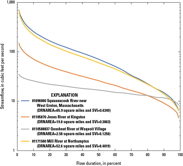
Example flow-duration curves at U.S. Geological Survey streamgages (A) Squannacook River near West Groton, Massachusetts (01096000; map number 12), (B) Jones River at Kingston, Mass. (01105870; map number 58), (C) Quashnet River at Waquoit Village, Mass. (011058837; map number 61), and (D) Mill River at Northampton, Mass. (01171500; map number 120). Streamgages are shown in figure 1 and described in table 1. DRNAREA, drainage area; SVI, streamflow variability index.
The USGS Hydrologic Toolbox software was used to compute flow durations (Barlow and others, 2022). The selected flow durations range from 99 to 1 percent (table 2), with the number of selected durations increasing in the extreme percentile ranges (from 99 to 90 and from 10 to 1). Estimated flow statistics at the 174 streamgages in the study for their periods of record are available in Bent and others (2025).
Table 2.
Selected streamflow statistics computed for regression analyses at U.S. Geological Survey streamgages used in and near Massachusetts.[POR, period of record; ABF, aquatic base flow; –, no regression equations determined for this study]
| Statistic | Analysis year | Description | Regression equations | |
|---|---|---|---|---|
| Mainland1 | Southeastern2 | |||
| 50 | Water year | 50th percentile of all daily mean discharges | Yes | Yes |
| 60 | Water year | 60th percentile of all daily mean discharges | Yes | Yes |
| 70 | Water year | 70th percentile of all daily mean discharges | Yes | Yes |
| 75 | Water year | 75th percentile of all daily mean discharges | Yes | Yes |
| 80 | Water year | 80th percentile of all daily mean discharges | Yes | Yes |
| 85 | Water year | 85th percentile of all daily mean discharges | Yes | Yes |
| 90 | Water year | 90th percentile of all daily mean discharges | Yes | Yes |
| 95 | Water year | 95th percentile of all daily mean discharges | Yes | Yes |
| 98 | Water year | 98th percentile of all daily mean discharges | Yes | Yes |
| 99 | Water year | 99th percentile of all daily mean discharges | Yes | Yes |
| June 50 | Water year | 50th percentile of the monthly medians; POR for complete months | Yes | – |
| June 90 | Water year | 90th percentile of the monthly medians; POR for complete months | Yes | – |
| July 50 | Water year | 50th percentile of the monthly medians; POR for complete months | Yes | – |
| July 90 | Water year | 90th percentile of the monthly medians; POR for complete months | Yes | – |
| August 50 | Water year | 50th percentile of the monthly medians; POR for complete months | Yes | – |
| August 90 | Water year | 90th percentile of the monthly medians; POR for complete months | Yes | – |
| September 50 | Water year | 50th percentile of the monthly medians; POR for complete months | Yes | – |
| September 90 | Water year | 90th percentile of the monthly medians; POR for complete months | Yes | – |
| 7Q2 | Climatic year | 2-year recurrence interval of the annual 7-day low-flow | Yes | – |
| 7Q10 | Climatic year | 10-year recurrence interval of the annual 7-day low-flow | Yes | – |
| 30Q2 | Climatic year | 2-year recurrence interval of the annual 30-day low-flow | Yes | – |
| 30Q10 | Climatic year | 10-year recurrence interval of the annual 30-day low-flow | Yes | – |
| Annual minima | Climatic year | Median of the annual 7-day low flow | Yes | – |
| Harmonic mean | Water year | Computed from the streamflow POR, and is generally smaller than the corresponding mean streamflow over POR, is adjusted for the days with zero flow, and gives greater weight to low daily mean streamflows than high daily mean streamflows (Rossman, 1990, and Koltun and Whitehead, 2002, equation 1) | Yes | – |
| February ABF | Water year | Median of monthly means over POR (Massachusetts Department of Conservation and Recreation, Office of Water Resources, 2008) | Yes | – |
| June ABF | Water year | Median of monthly means over POR (Massachusetts Department of Conservation and Recreation, Office of Water Resources, 2008) | Yes | – |
| August ABF | Water year | Median of monthly means over POR (Massachusetts Department of Conservation and Recreation, Office of Water Resources, 2008) | Yes | – |
Mainland regression equations are for Massachusetts, excluding the Plymouth-Carver Kingston-Duxbury aquifer system in southeastern Massachusetts and Cape Cod.
Southeastern regression equations are for the Plymouth-Carver Kingston-Duxbury aquifer system in southeastern Massachusetts and Cape Cod.
Flow durations represent the percentage of time that a given flow is equaled or exceeded without regard to the sequence of recorded flows (Searcy, 1959).
Other streamflow statistics—annual flow durations (40-, 30-, 25, 20-, 15-, 10-, 5-, 2-, and 1-percent), monthly 90- and 50-percent flow durations (January–May and October–December), and median of the monthly means (January, March–May, July, and September–December)—were computed for streamgages for the mainland area (Bent and others, 2025) and for streamgages and partial-record stations in the southeastern area (Sturtevant and others, 2025).
Low-Flow Frequency Statistics
Low-flow frequencies are computed for streamgages by determining the frequency of an annual series for a consecutive number of low-flow days (Riggs, 1972)—for example, the 7-day, 10-year low flow-frequency (7Q10). This statistic is the minimum consecutive D-day mean streamflow that is expected to occur once in any Y-year period, or that has a probability of 1/Y of not being exceeded in any given year. Any combination of number of days of mean minimum streamflow and years of recurrence may be used to determine the low-flow frequencies. The annual series for the determination of low-flow frequencies for this study was based on a climatic year. Use of a climatic year rather than a water year allows for an analysis of an uninterrupted low-flow period; in Massachusetts, this low-flow period typically occurs from early August through mid-October. The minimum number of climatic years of record for the streamgages was 8 years, although all streamgages used in the mainland and southeastern regression equations had 10 or more climatic years.
For this study, low-flow frequencies were computed for the 7-day, 2-year (7Q2); 7-day, 10-year (7Q10); 30-day, 2-year (30Q2); and 30-day, 10-year (30Q10) statistics (Bent and others, 2025). Low-flow frequencies were computed by using the USGS Hydrologic Toolbox software (Barlow and others, 2022). An example plot of the annual 7-day low-flows with the log-Pearson type III distribution fit is shown in figure 4. The 7Q2 and 7Q10 streamflow are where, in figure 4, the annual non-exceedance probabilities of 50 and 10 percent, respectively, intersect with the log-Pearson type III curve.

Graph showing example of the fit of the log-Pearson type III distribution to the annual 7-day low flow at the U.S. Geological Survey streamgage Quaboag River at West Brimfield, Massachusetts (01176000; map number 136 in fig. 1 and table 1), for climatic years 1913–2021. The 7-day, 2-year and 7-day, 10 year low-flow frequencies (7Q2 and 7Q10) are 32.4 and 14.2 cubic feet per second, respectively.
Annual, Monthly, and Other Statistics
The streamflow statistics harmonic mean, monthly flow duration, median of the monthly means, and the median of the annual 7-day low flow were computed by using R packages (Bent and others, 2025). Harmonic mean was computed with the R DVstats package (U.S. Geological Survey, 2024b) according to the EPA DFLOW user’s manual (Rossman, 1990). The median of the annual 7-day low-flows was computed from the annual 7-day low-flow, which was determined by using the USGS Hydrologic Toolbox software (Barlow and others, 2022).
Trends in Low-Flows
The traditional assumption underlying low-flow analysis is stationarity in time. The assumption allows researchers to estimate low-flow statistics from past records and apply them to the future without adjustments. Milly and others (2008) called the assumption of climate-related stationarity into question and advocated for new methods to replace models based on stationarity. Several studies have shown that streamflows can be nonstationary by documenting increases in low and median flows across the United States (McCabe and Wolock, 2002; Lins and Slack, 2005; Small and others, 2006; Hodgkins and Dudley, 2011; Dudley and others, 2020).
For the trend analysis, the annual 7-day low-flow data were analyzed for long-term trends at streamgages in and near Massachusetts by using the same methodology as Ahearn and Hodgkins (2020). Subsets of streamgages with longer records were created to evaluate trends during the periods of 30, 50, 70, and 90 climatic years up to 2019 (tables 3, 4, 5, and 6, respectively). All 10-year blocks within each time period analyzed were required to be at least 80 percent complete so that no part of the time series would have substantial missing data. These length and completeness criteria resulted in 64 streamgages for the 30-year period (1990–2019), 58 streamgages for the 50-year period (1970–2019), 43 streamgages for the 70-year period (1950–2019), and 14 streamgages for the 90-year period (1930–2019). The magnitudes of the trends were computed with the Sen slope (also known as the Kendall-Theil robust line). The Sen slope was calculated by determining the median of all possible pairwise slopes in each time series (Helsel and Hirsch, 2002). The Sen slope is multiplied by the number of annual 7-day low flows to obtain the magnitude of the trend or total change in the annual 7-day low flows over the period analyzed. For example, a Sen slope of 0.099 cubic foot per second per year multiplied by 70 for the 70-year period results in a trend of 6.92 ft3/s for the North River at Shattuckville, Mass. (01169000; map number 114 in fig. 1 and table 1) (table 5).
Table 3.
Trends for annual 7-day low flows for the 30-year period of climatic years 1990–2019 at U.S. Geological Survey streamgages used in this study in and near Massachusetts.[Map numbers of streamgages are shown in figure 1 and described in table 1. no., number; USGS, U.S. Geological Survey; ML, mainland; SE, southeastern; MA, Massachusetts; ft3/s, cubic foot per second; ft3/s/yr, cubic foot per second per year; NSS, not statistically significant using a 0.05 p-value; I, increase; NH, New Hampshire; R, River; BL, below; RI, Rhode Island; CT, Connecticut; VT, Vermont]
The mainland regression equations are for the area of Massachusetts excluding the Plymouth-Carver-Kingston-Duxbury aquifer system in southeastern Massachusetts and Cape Cod. The southeastern equations are for the Plymouth-Carver-Kingston-Duxbury aquifer system in southeastern Massachusetts and Cape Cod.
Table 4.
Trends for annual 7-day low flows for the 50-year period of climatic years 1970–2019 at U.S. Geological Survey streamgages used in this study in and near Massachusetts.[Map numbers of streamgages are shown in figure 1 and described in table 1. no., number; USGS, U.S. Geological Survey; ML, mainland; SE, southeastern; MA, Massachusetts; ft3/s, cubic foot per second; ft3/s/yr, cubic foot per second per year; NSS, not statistically significant using a 0.05 p-value; D, decrease; I, increase; NH, New Hampshire; R, River; BL, below; RI, Rhode Island; CT, Connecticut; VT, Vermont]
The mainland regression equations are for the area of Massachusetts excluding the Plymouth-Carver-Kingston-Duxbury aquifer system in southeastern Massachusetts and Cape Cod. The southeastern equations are for the Plymouth-Carver-Kingston-Duxbury aquifer system in southeastern Massachusetts and Cape Cod.
Table 5.
Trends for annual 7-day low flows for the 70-year period of climatic years 1950–2019 at U.S. Geological Survey streamgages used in this study in and near Massachusetts.[Map numbers of streamgages are shown in figure 1 and described in table 1. no., number; USGS, U.S. Geological Survey; ML, mainland; SE, southeastern; MA., Massachusetts; ft3/s, cubic foot per second; ft3/s/yr, cubic foot per second per year; NSS, not statistically significant using a 0.05 p-value; D, decrease; I, increase; NH, New Hampshire; R, River; BL, below; RI, Rhode Island; CT, Connecticut; VT, Vermont]
The mainland regression equations are for the area of Massachusetts excluding the Plymouth-Carver-Kingston-Duxbury aquifer system in southeastern Massachusetts and Cape Cod. The southeastern equations are for the Plymouth-Carver-Kingston-Duxbury aquifer system in southeastern Massachusetts and Cape Cod.
Table 6.
Trends for annual 7-day low flows for the 90-year period of climatic years 1930–2019 at U.S. Geological Survey streamgages used in this study in and near Massachusetts.[Map numbers of streamgages are shown in figure 1 and described in table 1. no., number; USGS, U.S. Geological Survey; ML, mainland; SE, southeastern; MA, Massachusetts; ft3/s, cubic foot per second; ft3/s/yr, cubic foot per second per year; BL, below; NSS, not statistically significant using a 0.05 p-value; D, decrease; I, increase]
The mainland regression equations are for the area of Massachusetts excluding the Plymouth-Carver-Kingston-Duxbury aquifer system in southeastern Massachusetts and Cape Cod. The southeastern equations are for the Plymouth-Carver-Kingston-Duxbury aquifer system in southeastern Massachusetts and Cape Cod.
The trends were computed with methods that consider the possibility of short-term persistence (STP) and long-term persistence (LTP) in the temporal data. This is an important issue that is often ignored in trend studies. Trends over time are sensitive to assumptions of whether underlying hydroclimatic data are independent, have STP, or have LTP (Cohn and Lins, 2005; Koutsoyiannis and Montanari, 2007; Hamed, 2008; Khaliq and others, 2009; Kumar and others, 2009). STP and LTP may represent the occurrence of wet or dry conditions that tend to cluster from year to year (Koutsoyiannis and Montanari, 2007; Hodgkins and others, 2017). For further discussion and references on persistence, refer to Hodgkins and Dudley (2011). Because the long-term time-series structure of low-flow data is not well understood, temporal trend significance with three different null hypotheses of the serial structure of the data is reported: independence, STP, and LTP (Hamed and Ramachandra Rao, 1998; Hamed, 2008). The serial structure of data referred to as “independence” means annual 7-day low flows from year to year are independent from each other (ignores any short or long clusters of wet and dry years). Trends were considered statistically significant at a p-value ≤0.05; this level represents a 5-percent probability that a trend is due to random chance. Results from the trend analyses for 30-, 50-, 70- and 90-year time periods under the three serial correlation structures, magnitudes of Sen slopes, and p-values are shown in tables 3 through 6. Low-flow trend results depend on the period of record analyzed and assumptions about the serial correlation structure of the annual peak flows.
For streamflow records influenced by regulation or other anthropogenic influences, interpretation of trend analyses is more complicated. Like near-natural sites, streamflow patterns at gages influenced by anthropogenic activities are also influenced by changes in climate patterns or basin characteristics. However, and this is especially true for regulated streamgages, those changes can be mitigated, enhanced, or even offset by changes in regulation patterns or other diversions. Nonetheless, trend assessments of flow patterns at such streamgages can be informative and, therefore, are included in these analyses.
For the 30-year period (1990–2019), 0 of the 24 streamgages used in the mainland regression analyses had statistically significant increasing or decreasing trends (p-value ≤0.05) if independence, STP, or LTP of 7-day annual low flows is assumed (table 3). For the southeastern regression analyses, one of two streamgages (Quashnet River at Waquoit Village, Mass.; 011058837; map number 61 in fig. 1 and table 1), had a statistically significant trend—increasing for independence and STP tests. For the other 38 streamgages not used in either of the regression analyses: 2 streamgages had a statistically significant increasing trend and 36 streamgages had no statistically significant trend for either independence, STP, or LTP tests.
For the 50-year period (1970–2019), 3 of the 21 streamgages used in the mainland regression analyses had statistically significant decreasing trends (p-value ≤0.05) (Nashoba Brook near Acton, Mass., 01097300, map number 17; Parker River at Byfield, Mass., 01101000, map number 26; and Branch River at Forestdale, Rhode Island, 01111500, map number 80—in fig. 1 and table 1) if independence, STP, or LTP of 7-day annual low flows is assumed (table 4). For the one streamgage in the southeastern regression analyses, there was no statistically significant trend. For the other 36 streamgages not used in either of the regression analyses: 3 streamgages had a statistically significant increasing trend, 5 had a decreasing trend, and 28 had no statistically significant trend in either independence, STP, or LTP tests. Two of these streamgages not used in either regression analyses also had statistically significant increasing trends for the 30-year period: Swift River at West Ware, Mass. (01175500; map number 134 in fig. 1 and table 1), and Deerfield River at Charlemont, Mass. (01168500; map number 113 in fig. 1 and table 1). Swift River at West Ware, Mass. (01175500), is downstream from Quabbin Reservoir, which is the water-supply for much of the Boston metropolitan area, and flows at Deerfield River at Charlemont (01168500) are affected by hydropower generation.
For the 70-year period (1950–2019), 4 of the 13 streamgages used in the mainland regression analyses had statically significant trends (p-value ≤0.05): 3 streamgages increasing and 1 streamgage decreasing if independence, STP, or LTP of 7-day annual low flows is assumed (table 5). No streamgages used in the southeastern regression analyses have period of records that go back 70 years. For the other 30 streamgages not used in either of the regression analyses: 6 streamgages had a statistically significant increasing trend, 2 had a decreasing trend, and 22 streamgages had no statistically significant trend in either independence, STP, or LTP tests. Only one of the streamgages also had statistically significant similar trends for the 30- and 50-year periods: increasing for Deerfield River at Charlemont, Mass. (01168500; map number 113 in fig. 1 and table 1).
For the 90-year period (1930–2019), only one streamgage was used in the mainland regression analyses, and it did not have a statistically significant trend for the other three assessments (table 6). No streamgages used in the southeastern regression analyses have periods of records that go back 90 years. For the other 13 streamgages not used in either regression analyses, 2 had statistically significant trends: 2 increasing and 2 decreasing in either independence, STP, or LTP tests. Only one of these streamgages also had similar statically significant trend for the 30-, 50-, and 70-year periods: increasing for Deerfield River at Charlemont, Mass. (01168500; map number 113 in fig. 1 and table 1), where flows are affected by hydropower generation.
As the science evolves and new data are obtained, further analysis could improve understanding of the trends observed in this study and the effects on low flows. Historical low-flow trends in and near Massachusetts do not offer clear and convincing evidence of the need to incorporate trends into low-flow analyses. If the evidence becomes clear, a well-defined deterministic mechanism should be identified prior to incorporating trends (Salas and others, 2018). For this study, the traditional assumption of stationarity is used with no adjustment for historical trends.
Basin Characteristics
The characteristics of streamflow are directly related to a drainage basin’s physical, land-cover, land-use, geologic, and climatological characteristics (table 7). Characteristics of the drainage basin were selected for use as potential explanatory variables in the regression analysis on the basis of their theoretical relations to low flows, the results of previous low-flow studies in similar hydrologic regions, and the feasibility of determining the basin characteristics with digital datasets and GIS technology. Measuring the basin characteristics with GIS technology facilitates automation of the process of solving the regional regression equations by using the USGS StreamStats web-based application.
Table 7.
Basin characteristics determined for drainage areas of U.S. Geological Survey streamgages used in this study in and near Massachusetts.[NAVD 88, North American Vertical Datum of 1988; SSURGO, Soil Survey Geographic Database; PRISM, Parameter-Elevation Regressions on Independent Slopes Model]
The basin boundaries delineated with StreamStats for the 174 streamgages in and near Massachusetts were overlaid on areal coverages of the basin characteristics of interest to determine the characteristics’ values for the basin upstream from each site (Bent and others, 2025). Basin, land-use, land cover, surficial geology, soil, and climatological characteristics were determined for the 174 streamgages in and near Massachusetts. These data and the sources of the GIS data are published in a USGS data release (Bent and others, 2025).
Streamflow Variability Index
Streamflow variability index (SVI) is a measure of the variability in streamflow resulting from variability in precipitation, as mitigated by characteristics of the basin such as surface storage and groundwater discharge (base flow). SVI has been found to be an explanatory variable in low-flow equations for recent studies in Alabama (Feaster and others, 2020), Iowa (Eash and Barnes, 2012), Kentucky (Martin and Ruhl, 1993; Martin and Arihood, 2010), Missouri (Southard, 2013), Ohio (Koltun and Whitehead, 2002; Whitehead, 2002; Koltun and Kula, 2013; VonIns and Koltun, 2024), and West Virginia (Friel and others, 1989). Unregulated streams with relatively small SVIs tend to have proportionally more flow contributed from groundwater discharge and (or) surface storage than streams with larger SVIs (Searcy, 1959). Figure 3 shows the flow duration curves for four selected streamgages and their associated calculated SVIs. Note that the Quashnet River at Waquoit Village, Mass. (011058837; map number 61 in fig. 1 and table 1), has a small SVI and has a relatively high more contribution to flow from groundwater discharge given that 95 percent of the drainage area is underlain by sand and gravel deposits (Sturtevant and others, 2025). Lane and Lei (1950) proposed SVI as a method to help produce synthetic flow-duration curves. The SVI is defined as the standard deviation of the logarithms of the 19 streamflow values at 5-percent class intervals from 5 to 95 percent on the daily flow-duration curve for the analysis period (Searcy, 1959). The formula for the SVI discussed in this report is
whereSVI
is the streamflow variability index, in logarithm of cubic feet per second;
Di
is the ith percent duration streamflow (i=95, 90, 85, … 5);
()
is the mean of the 19 streamflow values at 5-percent class intervals from 95 to 5 percent on the flow-duration curve of daily mean streamflows and
n
is the number of flow duration from the 95 to 5 percent in 5-percent class intervals, which is 19.
SVIs determined initially from streamgages with 8 or more water years of record in southern New England and eastern New York were plotted on a map (not shown) to assess spatial trends. Although there were visually identifiable spatial trends (for example, a cluster of low SVIs at streamgages in southeastern Massachusetts and Cape Cod—an area known for relatively high groundwater discharge)—it was apparent that, in some areas, SVIs can change appreciably over relatively small distances of 10–20 miles. Consequently, it was deemed important to compute and use as much SVI data as possible to prepare the grid. Therefore, in development of an SVI map for southern New England and eastern New York, SVI was computed at additional streamgages (some with periods of record less than 8 water years) and partial-record stations to improve the SVI map (Bent and others, 2025).
Koltun and Kula (2013) also estimated SVIs for other streamgages and partial-record stations in Ohio to assist in development of a detailed SVI map. Streamgages and partial-record stations within southern New England and eastern New York with published flow durations were added to the SVI database for creating the map (Bent 1995, table 5; Ries 1999, table 3; Bent, 1999, tables 8 and 9; Bent and others, 2014, tables 3 and 6). For the streamgages with a period of record less than 8 years, the flow-duration curve was used to compute the SVI for that streamgage. But for most of the partial-record stations, only flow durations from the 99th to 50th percentiles were available because they were mainly low-flow partial-record stations. Therefore, a relation between streamgages’ SVIs for the 10 flow durations in 5-percent class intervals from the 95th to 50th percentiles (SVI95–50) and the 19 flow durations in 5-percent class intervals from the 95th to 5th percentiles (SVI95–5) was developed (fig. 5). Development of this relation started with 304 streamgages with 8 or more water years of record in southern New England and eastern New York. During analyses, 56 streamgages were removed from the relation as they were determined to be outliers. Evaluation of these 56 streamgages’ flow-duration curves from the 99th to 1st percentiles showed clear changes that were associated with regulations, such as major water supply withdrawals, flood-control dams, and hydropower generation. The final relation between the SVI95–50 and the SVI95–5 was determined by using 248 long-term streamgages in southern New England and eastern New York (Bent and others, 2025). The relation is very good, with a coefficient of determination (R2) of 0.9583. The power regression equation for this relation was then used to estimate the SVI for the 95th- to 5th-percentile flow durations at partial-record stations that only have published flow durations from the 95th to 50th percentiles in 5-percent class intervals:
whereSVI95–5
is the streamflow variability index (SVI) based on 19 streamflows at the 95th to 5th percentile flow durations in 5-percent class increments, and
SVI95–50
is the streamflow variability index (SVI) based on 10 streamflows at the 95th- to 50th-percentile flow durations in 5-percent class increments.

Relation of the streamflow variability index (SVI) for the 95- to 50-percent flow durations to the SVI for the 95- to 5-percent flow durations, using U.S. Geological streamgages in southern New England and eastern New York.
SVI must be regionalized in some fashion to permit its estimation at ungaged sites. The geostatistical techniques of kriging, inverse distance weighting, and natural neighbor were all examined as possible methods for regionalizing SVI (Esri, 2023c). Maps of SVI regionalized by geostatistical techniques were developed by using 664 sites (276 streamgages with 8 or more water years of record, 102 streamgages with less than 8 water years of record, and 286 partial-record stations) in and near southern New England and eastern New York (Bent and others, 2025). Of the 276 streamgages with 8 or more water years of record, 28 streamgages were just outside the southern New England and eastern New York area. These streamgages were included to make sure that the drainage areas of streamgages on the perimeter of the area being used in the regression analyses would be covered by the map to determine a mean basin SVI. Evaluation of maps of the regional SVI for southern New England and eastern New York created using the geostatistical techniques determined kriging to be the most representative method (Esri, 2023b). Kriging is based on statistical models that include autocorrelation, which is the statistical relations among the measured data points (Esri, 2023a). Kriging fits a specified number of data points within a specified radius to determine output values. It has multiple steps, including exploratory statistical analyses, variogram modeling, and creating the output values. Kriging is often used when there is spatial correlation or bias in the data, especially with soil and geologic related data. Thus, kriging is appropriate for SVI data. The final SVI grid for southern New England and eastern New York is illustrated in figure 6. This SVI grid was used to determine a mean SVI value for each streamgage’s drainage area in and near southern New England. The mean basin SVI values for the 174 streamgages tested for possible use in the regression analyses are in Bent and others (2025).

Streamflow variability index (SVI) map developed from kriging techniques for southern New England and eastern New York.
Comparison of the mean SVI values from kriging to the computed at-site SVI values using equation 2 was possible at 135 of the 174 streamgages. Of the 39 streamgages not used in the comparison, 37 sites had regulations, such as major water supply withdrawals, flood-control dams, and hydropower generation; and for 2 sites on Cape Cod, an accurate surface-water drainage area could not be determined. The average and median of the mean SVI values were 0.468 and 0.464, respectively, which compared well to the average and median of the at-site SVI values of 0.472 and 0.464, respectively, for the 135 streamgages.
Methods for Estimating Selected Low-Flow Statistics in Mainland Massachusetts
Streamflow information for ungaged sites is critical for Federal, State, county, city, and town agencies; nongovernmental and private organizations; and individuals and public groups dealing with water-resources issues. Flow-frequency and duration-streamflow statistics for streams at ungaged sites can be estimated by several methods. These methods include the use of (1) a drainage-area ratio and (2) a regression equation relating streamflow statistics to basin characteristics.
Drainage-Area Ratio Methods
The drainage-area ratio method is based on the assumption that the near-natural (minimal to no regulations) streamflow at an ungaged site is the same per unit of drainage-basin area as that at a nearby hydrologically similar streamgage with near-natural flows. Drainage areas of the ungaged site and the streamgage are determined from topographic maps or the USGS StreamStats web-based application (https://streamstats.usgs.gov/ss/). Streamflow statistics are computed for the streamgage, and then the statistics (streamflow values) are divided by the drainage area to determine the streamflow for each statistic per unit area, in cubic feet per second per square mile, at the streamgage. These values are multiplied by the drainage area to the ungaged site to obtain estimated statistics for that site. This method is most commonly applied if the index streamgage is on the same stream as the ungaged site because the accuracy of the method depends on the proximity of the two sites, on similarities in drainage area, and on other physical and climatological characteristics of their drainage basins.
Several studies have provided estimates of the maximum difference in drainage areas for which the use of the drainage-area ratio method would generate more accurate estimates of streamflow statistics than the use of regression equations. Guidelines have been provided for estimating peak-flow statistics, and usually the recommendation has been that the drainage area to the ungaged site should be 0.5 to 1.5 times the drainage area of the index streamgage (Choquette, 1988, p. 41; Koltun and Roberts, 1990, p. 6; Lumia, 1991, p. 34; Bisese, 1995, p. 13; Koltun and Whitehead, 2002, p. 22; Martin and Arihood, 2010, p. 28). Koltun and Schwartz (1987, p. 32) recommended a narrower range of 0.85 to 1.15 times the drainage area of the index streamgage for estimating low flows at ungaged sites in Ohio. Ries and Friesz (2000), however, determined that the drainage-area ratio method could be used to estimate low-flow statistics for ungaged sites in Massachusetts if the drainage area for an ungaged site was between 0.3 and 1.5 times the drainage area of the index streamgage site. They found that this method was generally as accurate as, or more accurate than, regression equations for this range of drainage areas.
In the drainage-area ratio method, the streamflow values are transferred from a streamgage to the ungaged site by the following formula:
whereQu
is the estimated streamflow at the ungaged site,
Qg
is the streamflow at the streamgage,
DRNAREAu
is the drainage area at the ungaged site, and
DRNAREAg
is the drainage area at the streamgage.
Eash and Barnes (2012) compared estimates of the 7-day, 10-year low flow developed by using regional regression equations, the drainage-area ratio method, and the weighted drainage-area ratio method to estimates from streamflow records for 48 streamgages (31 pairs of streamgages) on rivers in Iowa. They found that the weighted drainage-area ratio provided the best estimate if the drainage area to the ungaged site was between 0.4 and 1.5 times the drainage area of the streamgage.
In the weighted drainage-area ratio method, the streamflow values are transferred from a streamgage to the ungaged site by using the following formula:
whereQuw
is the weighted estimated streamflow at the ungaged site,
Qur
is the streamflow at the ungaged site estimated from the regression equation,
Qgs
is the streamflow at the streamgage estimated from measured data,
Qgr
is the streamflow at the streamgage estimated from the regression equation,
|DRNAREA|
is the absolute value of the difference between the drainage areas to the streamgage (DRNAREAg) and the ungaged site (DRNAREAu),
DRNAREAg
is the drainage area to the streamgage, and
DRNAREAu
is the drainage area to the ungaged site.
As the ratio (Qgs/Qgr) approaches 1, or the ratio of DRNAREAu to DRNAREAg approaches 0.5 or 1.5, the weighting factor in equation 5 approaches 1 and it no longer has an effect on the regression equation estimate for the ungaged site (Qur). Additionally, both the drainage-area and weighted drainage-area ratio methods may not be applicable for ungaged sites where physical, land-cover, land-use, surficial-deposit, or climatological characteristics or regulations are substantially different between the ungaged site and the streamgage. The error associated with estimates based on the drainage-area and weighted drainage-area ratio methods cannot be calculated.
Regional Regression Analysis
Studies to develop regional regression equations for estimating streamflow statistics at ungaged sites have been done in many States throughout the United States, including those adjacent to Massachusetts (refer to the report section “Previous Studies”). Multiple regression analyses provide a mathematical equation for estimating a response (dependent) variable—that is, a streamflow statistic—from one or more explanatory (independent) variable(s), such as basin characteristics. Ideally, the development of regression equations involves the use of streamflow data from a large number of long-term streamgages on unaltered streams evenly distributed across the region of interest and with a range of basin characteristics. But in many cases, the number of streamgages representing unaltered flow is limited, the streamgage network is biased toward representing larger streams or rivers, the network is unevenly distributed geographically, and the range of basin characteristics upstream from streamgages does not cover the complete range found in the region. In Massachusetts, the number of streamgages on streams with minimal to no regulations is limited; for this reason, nearby streamgages in the surrounding States within about 25 miles of the border were used. The daily mean streamflow records at these streamgages were used to compute selected low-flow statistics, and then those statistics and basin characteristics at these streamgages were used to develop regional regression equations for estimating selected low-flow statistics at ungaged sites in Massachusetts.
Multiple regression is used to create equations that relate streamflow statistics for streamgages to the physical, land-cover, land-use, surficial-deposit, soil, and climatological characteristics of their upstream drainage areas. Once an optimal equation has been determined, a streamflow statistic at a nearby ungaged site in a basin with similar characteristics can then be estimated by applying the equation to the ungaged site.
The basic equation describing a linear multiple regression analysis is
whereYi
is the response (dependent) variable (an estimated streamflow statistic) for the ungaged site i,
b0 to bn
are the coefficients determined in the analysis,
Xi to Xn
are the explanatory (independent) variables (basin characteristics) for the ungaged site i, and
ei
is the residual error or difference between the observed and estimated response variables for ungaged site i.
Linear regression analysis is based on the following assumptions: (1) the mean of the residuals (ei) is zero, (2) the variance of the residuals is constant, (3) the residuals are normally distributed, and (4) the residuals are independent of each other. In addition to these assumptions, the selected explanatory variables (X) should have a physical basis as predictors of the streamflow statistic, the explanatory variables (basin characteristics) in the equation should not be highly correlated with each other, and the signs of the terms of the equation should make hydrological sense. For example, the variable drainage area should have a positive coefficient because an increase in drainage area should result in an increase in the value of the streamflow statistic.
In almost all regionalization studies to determine low-flow and peak-flow statistics, the response and explanatory variable datasets are skewed. As a consequence, the data need to be transformed to ensure that the mean of the residuals equals zero. In many studies, a logarithmic transformation is used. A base-10 log-transformed multiple regression equation has the form
After the coefficients have been determined through regression analysis, the equation is transformed back to its original units in a form that can be used to estimate a specific streamflow statistic at an ungaged site. The retransformed equation has the following form:
A linear regression equation provides an unbiased estimate of the mean response of the response variable. Although estimates provided by equation 7 are unbiased, these estimates are in log units, whereas estimates in the original units are needed to calculate specific streamflow statistics at an ungaged site. Estimates from equation 8 are in the original units. However, this equation predicts the median, instead of the mean, value of the response variable. A streamflow statistic based on a median creates an estimate that is biased and tends to be lower than the mean (Ries and Friesz, 2000). Bias correction factors (BCFs) were used in some studies in Massachusetts and New Hampshire to remove the bias from the estimate (Ries, 1994a, b; Ries and Friesz, 2000; Flynn, 2003a, b; Archfield and others, 2010). In other studies (Risley, 1994; Stuckey, 2006; Armstrong and others, 2008; Ahearn, 2010), BCFs were not used because they were generally very small. In this study, BCFs were also not used because if they were, then the streamflows estimated from the regression equations would not have an equal chance of being higher or lower than their actual values (Julie Kiang, U.S. Geological Survey, oral commun., 2011).
Development of Regression Equations
In regional regression studies, explanatory and response variables often need to be transformed before the regression equation is created to ensure a linear relation. Scatterplots, correlation tables, and linear regression analyses were done by applying the statistical software TIBCO Spotfire S+ 8.1 for Windows (TIBCO Software, Inc., 2008) to the selected low-flow statistics at the 81 streamgages (Bent and others, 2025) and the basin characteristics (Bent and others, 2025) to determine if variable transformations were needed (Farmer and others, 2019). The scatterplots indicated that a log transformation was needed to meet the assumptions of linear regression. Therefore, the logarithmic (base-10) transformation was selected and applied to streamflow statistics (response variables) and basin characteristics (explanatory variables) to linearize the relation between the explanatory variables and the response variables, to ensure equal variance about the regression line, and to decrease the spread of the data. Several potential explanatory variables (basin characteristics) for the drainage basin upstream from a few streamgages had one or a few values of zero. The variables were generally limited to land-cover, land-use, soil, or surficial deposit characteristics of the drainage basin, such as forested land, water bodies, wetlands, storage, developed land, Soil Survey Geographic Database (SSURGO) hydrologic soil groups, and surficial geology. To logarithmically (base-10) transform all the values of that basin characteristic, a constant value of 0.10 was added to all values of the characteristic. Scatterplots of logarithmically (base-10) transformed basin characteristics were then examined to determine if particular characteristics were correlated with other characteristics. If two basin characteristics were found to have a moderate or strong correlation with an absolute value of Pearson’s correlation coefficient (r) greater than or equal to 0.50, then those basin characteristics were tested separately in the variable-selection process of the regression analyses. This separate testing was done to eliminate redundant basin characteristics in the variable-selection process.
For the initial regression analyses of the selected potential explanatory variables, the automated statistical procedures called “subset selection” were used in TIBCO Spotfire S+ 8.1 for Windows (TIBCO Software, Inc., 2008). The selection procedures determined the statistical combination that was entered in the equation for each of the explanatory variables (basin characteristics), and variables were retained or deleted on the basis of their statistical importance. In the procedure “best subsets,” the equations with the highest adjusted R2, the Mallows’ Cp closest to the number of explanatory variables plus the constant 1, the lowest residual standard error, and the predicted residual error sum of squares (PRESS) statistics were evaluated for each of the possible combinations of selected explanatory variables to determine the best possible combinations of the explanatory variables. The procedure identified the best combinations of explanatory variables for models with one, two, and three explanatory variables.
The top few potential explanatory variables identified in the subset selection were further evaluated with the ordinary least-squares (OLS) regression procedure. No explanatory variables that were highly correlated (absolute value of r greater than or equal to 0.50) were included in the same equation. For the OLS regression procedure, the explanatory variables’ p-values and t-statistic values were evaluated to determine those to be less than or equal to 0.05 and to have absolute values greater than or equal to 2.00, respectively. Graphical output for the OLS regression procedure was evaluated for model fit as well as influential outliers. The graphical output included plots of the residuals (difference between the actual streamflow statistic and the fitted value) versus the fitted (predicted) values; the actual streamflow statistic values versus the fitted values; residuals versus the quartiles of the standard normal distribution; and the Cook’s distance for each streamgage (TIBCO Software, Inc., 2008). Additionally, regression equations with two or three explanatory variables were compared to determine if the equations were significantly improved by adding an additional explanatory variable.
In the initial evaluations of the regression equations, hydrologic regions were also evaluated to determine if regional equations would be more accurate than statewide equations. Hydrologic regions refer to areas in which streamgages indicate a similarity of flow response that differs from the flow response in adjacent regions. Potential hydrologic regions were evaluated by dividing the streamgages in southern New England and eastern New York into separate regions based on broad physiographic regions (Denny, 1982) and level III ecoregions (U.S. Environmental Protection Agency, 2022b). These regions are based on similarities in topography, geology, and (or) ecosystems. In addition, streamgages in eastern and western Massachusetts were evaluated as separate hydrologic regions, divided by the Connecticut River, similar to regions in Ries and Friesz (2000). Eight-digit hydrologic unit code (HUC8) boundaries were followed wherever possible to avoid dividing basins into multiple regions. Error metrics (mean square error, MSE, and root mean square error, RMSE) that are commonly used for evaluating and reporting the performance of regression models were used in assessing model performance based on the hydrologic regions tested for this study. No clear improvements in the performance metrics were found to warrant regional equations based on the hydrologic regions tested.
Final Regression Equations
The final regression equations were determined by using the technique in the weighted-multiple-linear regression (WREG) program (Eng and others, 2009) and left-censored regression (Kroll and Stedinger, 1999). This was done by using the R package for WREG (Farmer, 2023) and the R package for left-censored regression (Lorenz, 2015).
The final regression equations for the flow-duration statistics from 99 to 50 percent; June to September 90- and 50-percent flow duration; median of the February, June, and August means; harmonic mean; and median of the annual 7-day low flow were developed by using weighted least-squares (WLS) regression. WLS is used for these low-flow statistics because they are not frequency statistics that involve the log-Pearson type III distribution for their estimation.
For the low-flow frequency statistics 30Q2 and 30Q10, the final regression equations were developed by using generalized least-squares regression (GLS). GLS requires the skew, K, and standard deviation for the log-Pearson type III distribution (Eng and others, 2009), which were computed by using the USGS Hydrologic Toolbox (Barlow and others, 2022).
For the low-flow frequency statistics 7Q2 and 7Q10, the final regression equations were developed by using weighted left-censored regression. This was because, for the 7Q2 statistic, 1 of 81 streamgages had a flow value of zero and, for the 7Q2 statistic, 5 streamgages had flow values of zero. The value of zero cannot be logarithmically transformed, but logarithmic transformation of streamflow statistics (that are not normally distributed) is needed to develop regression equations. The method of handling the zero values in a regression analysis depends on the number of streamgages in the dataset with response variables equal to zero. If the number is small, left-censored regression analysis is used: either an adjusted maximum-likelihood estimation (Cohn, 1988; Helsel, 2005) or a censoring method that adds a small constant value (0.01, 0.10, and 1.00) to all response variables in a dataset (Kroll and Stedinger, 1999). Censoring and coding data as “less than” a threshold value (0.01, 0.10, and 1.00) allows the use of a log transformation on the data and, therefore, allows all the data (uncensored and censored) to be used in the regression analysis to develop the regional equations (Watson and McHugh, 2014). For the 7Q2 and 7Q10 regression analyses, a small constant value of 0.01 (censoring threshold value of 0.01 ft3/s) was used because this is the lowest flow value reported by the USGS. Weighted left-censored regression techniques were used for the final regression analyses, with the weights being based on the number of years of record at the streamgages (Ziegeweid and others, 2015; Gotvald, 2017; Feaster and others, 2020).
The regression analyses determined that drainage area (represented by the variable DRNAREA) was a significant explanatory variable (p-value less than or equal to 0.05) in all 27 of the regression equations. Drainage area generally is the most significant explanatory variable in all regional streamflow regression equations, whether for low flows; peak flows; or mean annual, mean monthly, or median monthly statistics. The final regression equations for the 27 streamflow statistics are listed in table 8.
Table 8.
Summary of regression equations and measures of model accuracy for estimating selected streamflow statistics for the mainland area of Massachusetts (excludes the Plymouth-Carver-Kingston-Duxbury aquifer system area in southeastern Massachusetts and Cape Cod).[Flow duration is the percentage of time that streamflow was equaled or exceeded. R2, coefficient of determination; MSE, mean square error in log-base 10 logarithm; RMSE, root mean square error, in percent; DRNAREA, drainage area in square miles; SOILAB+0.1, percent area of the combined Soil Survey Geographic Database (SSURGO; Natural Resources Conservation Service, 2022) hydrologic soil type A and B plus the value of 0.1 to ensure there are no zero values; WLS, weighted least-squares regression; WREG, weighted-multiple-linear regression (Eng and others, 2009); SVI, streamflow variability index (unitless); TEMP, mean annual temperature; GLS, generalized least-squares regression]
The SVI (unitless) was a significant explanatory variable (p-value less than or equal to 0.05) in 20 of the 27 regression equations and was in the equations estimating lower streamflow statistics (for example, the 99- to 75-percent flow durations). The combined percentage of SSURGO hydrologic soil groups A and B (SOILAB) was a significant explanatory variable in the remaining 7 of the 27 regression equations, and this variable tended to be in the equations estimating more moderate streamflow statistics (for example, the 70- to 50-percent flow durations). Mean annual temperature from 1981 to 2010 (TEMP) was in one equation, to estimate the February median of the monthly means.
As noted previously, several recent low-flow studies have SVI as an explanatory variable for low-flow statistic regression equations—for example, in Alabama, Iowa, Kentucky, Ohio, and West Virginia. Both hydrologic soil groups A and B were explanatory variables in low-flow equations in Iowa (Eash and Barnes, 2012).
The coefficient for SVI was negative in the 20 regression equations it was in, and the coefficient was more negative for the lower streamflow statistics, −4.7437 coefficient at the 99-percent flow duration and −1.4915 coefficient at the 75-percent flow duration (table 8). As shown in figure 3, streamgages with larger SVIs (for example, Squannacook River near West Groton, Mass.; 01096000; map number 12 in fig. 1 and table 1) tend to have a flow-duration curve with a steeper slope. In order to reduce the larger SVI values, the coefficient needs to become more negative as the streamflows get lower.
The coefficient SOILAB was positive in all the regression equations, which is expected because hydrologic soil group A consists of well-drained sands and gravelly sands with high infiltration and low runoff rates and group B consists of well-drained, moderately fine to moderately coarse-textured soils with moderate rates of infiltration and runoff (Esri, 2022). SOILAB tends to be located in areas with more sand and gravel, alluvium, and fine sand surficial deposits, and therefore those areas tend to have higher contributions from groundwater discharge (base flow) at the lower streamflows. SOILAB is shown in the regression equations as SOILAB+0.1 (table 8). This is to ensure that no SOILAB value could be zero, because a value of zero cannot be logarithmically transformed.
Mean annual temperature (TEMP) was a positive coefficient in the regression equation for the February median of the monthly means (table 8). During February, those areas with higher mean annual temperatures may have more runoff, due either to more precipitation as rain rather than snow or to more snowmelt, than areas with slightly colder mean annual temperatures.
The RMSE for the 27 regression equations ranged from 17.85 to 130.70 percent (table 8). The low-flow statistics—the 99- and 98-percent flow durations, August and September 90-percent flow durations, and 7Q10 and 30Q10—had standard errors of the estimate greater than 100 percent. Generally, the higher the flow statistic, the lower the standard error of the estimate. Although the standard errors of the estimate are high for the lower flow statistics, they were similar to those calculated for regional regression equations developed to estimate low-flow statistics in Rhode Island (Bent and others, 2014), Connecticut (Ahearn, 2010), and Massachusetts (Ries and Friesz, 2000), and in other USGS low-flow studies.
Review of areal plots (not shown) of the residuals (differences between streamflow statistics estimated from measured streamflow and those estimated from the regression equations) for selected low-flow frequencies and durations at the 81 streamgages did not indicate any strong regional biases (clear groups of negative or positive residuals). Additionally, plots of the streamflow statistics estimated from measured streamflow (observed data) as functions of the same statistics estimated from the regression equations (predicted data) are presented in figures 7A–G. These plots show no clear bias of the streamflow values generated by regression equations with respect to measured streamflows versus predicted values. However, at lower flows (7Q10, 99-percent flow duration, 30Q2, and 90-percent flow duration), the range of the data is clearly wider than that for slightly higher low-flows (median of the monthly means for August, harmonic mean, and June 50-percent flow duration). Again, a wide range between observed and predicted data is generally found in all low-flow studies, especially for the equations for estimating lower flows with the higher percent RMSE—for example, equations where the RMSE is greater than 50 percent (table 8).

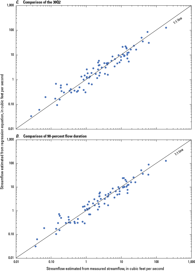
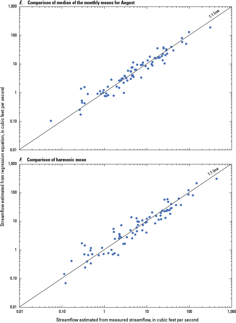
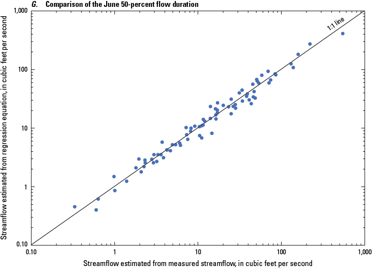
Graphs showing comparisons of the (A) 7-day, 10-year low-flow frequency (7Q10), (B) 99-percent flow duration, (C) 30-day, 2-year low-flow frequency (30Q2), (D) 90-percent flow duration, (E) median of the monthly means for August, (F) harmonic mean, and (G) June 50-percent flow duration estimated from measured streamflow and the mainland regression equations for U.S. Geological Survey streamgages in and near Massachusetts. The mainland area of Massachusetts excludes the Plymouth-Carver-Kingston-Duxbury aquifer system area in southeastern Massachusetts and Cape Cod.
Prediction Intervals
Prediction intervals indicate the uncertainty inherent in use of the equations. At the 90-percent confidence level, prediction intervals can be calculated for estimates obtained from the regression equations. There is a 90-percent probability that the true value of the streamflow statistic for an ungaged site will be within the prediction interval (Ries and Friesz, 2000). The lower and upper boundaries of the 90-percent prediction intervals can be computed by
whereQ
is the estimated streamflow statistic for the site,
QLPI
is the estimated lower boundary of the 90-percent prediction interval,
QUPI
is the estimated boundary of the upper 90-percent prediction interval, and
T
is the 90-percent prediction interval determined from equation 10:
t (α/2, n−p)
is the critical value from the Student’s t distribution,
α
is the alpha level (α = 0.10 for 90-percent prediction intervals),
n−p
is the number of degrees of freedom with n data values (number of streamgages) used in the regression analysis,
p
is the number of parameters in the equation (equal to the number of explanatory variables or basin characteristics plus 1), and
Si
is computed from equation 11, below.
Critical values from the Student’s t distribution are listed in many introductory statistics textbooks. The value of Si is computed by using the equation
whereγ2
is the model-error variance (equal to the root mean square error (RMSE) squared),
xi
is a row vector of the logarithms of the basin characteristics for site i which has been augmented by a 1 as the first element,
U
is the covariance matrix for the regression coefficients, and
xi'
is the transpose of xi (Ludwig and Tasker, 1993).
The values of t(α/2, n−p) and U needed for equations 10 and 11 for the 21 regression equations are presented in table 9. The value of γ2 needed in equation 11 is the value of the MSE (base-10 logarithm) in table 9.
Table 9.
Information needed for calculation of the 90-percent prediction intervals for estimates of selected statistics calculated by regression equations for streamflows in the mainland area of Massachusetts (excludes the Plymouth-Carver-Kingston-Duxbury aquifer system area in southeastern Massachusetts and Cape Cod).[Flow duration is the percentage of time that streamflow was equaled or exceeded. no., number; p, number of parameters is equal to the number of explanatory variables plus 1; t, Student’s t distribution using an alpha of 0.10 and 77 or 78 degrees of freedom (number of streamgages – p, only the February median of the monthly means has 77 degrees of freedom and all other equations have 78 degrees of freedom); WLS, weighted least-squares regression; MSE, mean square error; log, base-10 logarithm; RMSE, root mean square error; %, percent; U, covariance matrix for the regression coefficients; DRNAREA, drainage area in square miles; SOILAB, percent area of Soil Survey Geographic Database (SSURGO; Natural Resources Conservation Service, 2022) hydrologic soil groups A and B plus 0.1; SVI, streamflow variability index; Aug., August; Sept., September; Feb., February; TEMP, mean annual temperature in degrees Fahrenheit; 7Q2, the annual minimum average streamflow for 7 consecutive days that has a 0.50 probability of not being exceeded in a given year; 7Q10, the annual minimum average streamflow for 7 consecutive days that has a 0.10 probability of not being exceeded in a given year; 30Q2, 30-day, 2-year low-flow frequency; 30Q10, 30-day, 10-year low-flow frequency]
Development of Low-Flow Statistics and Basin-Characteristic Datasets for Southeastern Massachusetts and Cape Cod
The Plymouth-Carver-Kingston-Duxbury aquifer system of southeastern Massachusetts and Cape Cod (fig. 8) is distinctly different hydrologically from other parts of Massachusetts. Southeastern Massachusetts and Cape Cod have glacially derived aquifers, which compose the largest groundwater reservoir in the State (Masterson and Walter, 2009). These coastal aquifers are the sole source of water for many municipalities and the primary source of water for streams, kettle-hole ponds, and wetlands in the region. The groundwater discharge from these aquifers also maintains the ecology of the coastal estuaries and salt marshes.
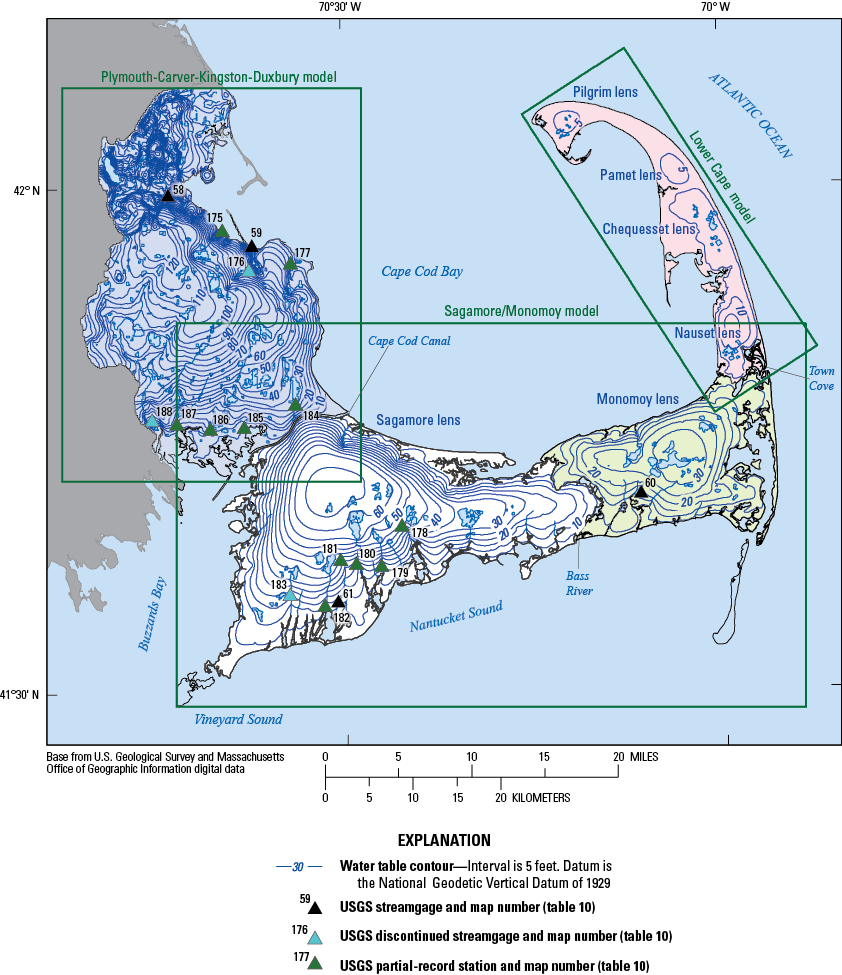
Locations of 7 U.S. Geological Survey streamgages and 11 U.S. Geological Survey partial-record stations in the Plymouth-Carver-Kingston-Duxbury aquifer system area in southeastern Massachusetts and on Cape Cod. U.S. Geological Survey streamgages and partial-record stations are described in table 10. Figure modified from Walter and others (2016).
For the Plymouth-Carver-Kingston-Duxbury aquifer system of southeastern Massachusetts and Cape Cod, the groundwater contributing areas and surface-water drainage areas do not always coincide because of the hydrogeology of this area (Masterson, 2004; Masterson and others, 2009; Walter and others, 2016). In these areas, groundwater can flow from one surface-water drainage area into another; therefore, for basins whose groundwater contributing areas are larger than their surface-water drainage areas, the mainland equations would likely underestimate streamflows. Conversely, for areas whose groundwater contributing areas are smaller than their surface-water drainage areas, the mainland equation would likely overestimate streamflows. Thus, the mainland regression equations are not applicable to this area of the State because of its known appreciable differences between surface-water drainage areas and groundwater contributing areas, and a different set of equations are needed to estimate selected low-flow statistics.
Currently (2025), no “southeastern” Massachusetts regional regression equations exist within USGS StreamStats for estimating selected streamflow statistics at ungaged sites in the Plymouth-Carver-Kingston-Duxbury aquifer system of southeastern Massachusetts and on Cape Cod. Tasker (1972) developed regression equations to estimate the low-flow statistics—7Q2 and 7Q10—in the Taunton River Basin and Plymouth-Carver aquifer system of southeastern Massachusetts based on the surface-water drainage area and a groundwater factor. The three groundwater factors were the area of the basin where wells generally (1) yield more than 300 gallons per minute (gal/min), (2) yield between 100 and 300 gal/min, and (3) yield less than 100 gal/min. The study found that by including average groundwater available from wells, the error was significantly reduced relative to regression equations with only surface-water drainage area for estimating the 7Q2 and 7Q10.
Selected at-site streamflow statistics have been summarized for selected streamgages whose periods of record are shorter (for this study less than 8 years, hereafter referred to as “short-term streamgage”) and partial-record stations in the Plymouth-Carver-Kingston-Duxbury aquifer system by Wandle and Morgan (1984), Bent (1995), Ries (1999), and Masterson and others (2009, app. 3). On Cape Cod, flow data at short-term streamgages and partial-record stations have primarily been used in conjunction with water-quality samples, groundwater seepage runs, and for calibration of groundwater models. Some limited streamflow statistics have been published for several sites on Cape Cod (Ries, 1999). Selected streamflow statistics for the four long-term streamgages in the Plymouth-Carver-Kingston-Duxbury aquifer system and on Cape Cod (fig. 8) are available in the USGS National Water Information System (NWIS) and USGS StreamStats.
The Plymouth-Carver-Kingston-Duxbury aquifer system is an unconfined, mainly sand and gravel aquifer and is the second largest aquifer system in Massachusetts. The aquifer contains more than 500 billion gallons of freshwater (Williams and Tasker, 1974a). It is composed mostly of glacially deposited sediments ranging in size from clay to boulders, and it ranges in thickness from less than 20 to more than 200 ft (Hansen and Lapham, 1992). Groundwater discharge from the aquifer supports numerous kettle ponds and coastal streams. The aquifer was designated as a sole source aquifer by the EPA, a recognition that groundwater is a vital source of drinking water for many of the communities in the area. Extensive water-resources studies of all or parts of the Plymouth-Carver-Kingston-Duxbury aquifer system have been completed by Williams and Tasker (1974a, b), Williams and others (1975, 1977), Hansen and Lapham (1992), Bent (1995), Masterson and others (2009), Carlson and others (2017), and U.S. Geological Survey (2024a).
Cape Cod is underlain by sand and gravel sediments and is an unconfined aquifer that is the sole source of freshwater for local municipalities. Cape Cod has six hydraulically distinct groundwater flow systems (Barbaro and others, 2014). Barbaro and others (2014) reported that in most areas of Cape Cod, the groundwater in sand and gravel aquifers is shallow, and about 69 percent of the water discharges to the coast, 24 percent discharges to streams, and the remaining 7 percent is withdrawn for public water supplies. Numerous Cape Cod water-resources studies have been completed over the last 50-plus years by the USGS and others (U.S. Geological Survey, 2024a).
The Sagamore/Monomoy groundwater model area for Cape Cod is between the Cape Cod Canal and the elbow of Cape Cod and has two separate freshwater flow lenses—Sagamore and Monomoy (west to east, fig. 8), which consist of unconsolidated glacial sediments (Walter and Whealan, 2005). The unconfined Sagamore and Monomoy aquifer systems are surrounded by saltwater—Buzzards Bay (west), Cape Cod Bay (north), and Nantucket Sound (south). The Sagamore and Monomoy lenses are hydraulically separated by the Bass River, which is along the border between the towns of Yarmouth and Dennis (not shown). The Sagamore lens on western Cape Cod is bounded at its northwest extent by the Cape Cod Canal, and the Momonoy lens is bounded at its northeast extent by Town Cove, which borders the towns of Orleans and Eastham (not shown). Depth to bedrock ranges from 50 to 900 ft below NAVD 88, and glacial deposits overlying the bedrock range in thickness from 70 to 500 ft (Walter and Whealan, 2005).
The Lower Cape groundwater model area for Cape Cod is between the towns of Eastham and Provincetown (not shown) and has four separate freshwater flow lenses—Nauset, Chequesset, Pamet, and Pilgrim (south to north, fig. 8), which are bound laterally and below by saltwater (Masterson, 2004). Groundwater flows radially from the tops of the groundwater mounds of each of the four lenses towards the coast and towards the inter-lens surface-water discharge areas (Masterson, 2004). Depth to bedrock ranges from 450 to 900 ft below NAVD 88, and the depth to the freshwater/saltwater interface of the aquifers is as much as 400 ft below NAVD 88.
The groundwater models used to determine the areas contributing recharge directly to individual stream reaches or reachsheds (Timothy McCobb, U.S. Geological Survey, written commun., 2024; hereafter referred to as “groundwater contributing areas) to the long- and short-term streamgages and partial-record stations and all stream cells were the Plymouth-Carver-Kingston-Duxbury aquifer system model (Masterson and others, 2009), the Sagamore/Monomoy model (LeBlanc and others, 2019), and the Lower Cape model (Nauset, Chequesset, Pamet, and Pilgrim lenses) (Masterson, 2004) (fig. 8). The groundwater contributing areas were determined by using the new MODPATH version 6 (Pollock, 2012) water-particle-tracking simulations. In these MODPATH version 6 simulations, water-particle endpoints associated with unique hydrologic model cells (200 by 200 ft) representing streams in the groundwater models were identified by tracking the movement of water particles through the simulated hydrologic system. This simulation was run such that any groundwater flow into a water body remained in the water body and only flowed out through the outflow point of the water body (that is, no groundwater was allowed to move out of the water body to an adjacent aquifer). Methods and data for the groundwater contributing areas for all hydrologic model cells representing streams cells in the three models, representing the streams in the Plymouth-Carver-Kingston-Duxbury aquifer system model and those streams on Cape Cod in the Sagamore/Monomoy and Lower Cape models, are available in associated USGS data releases (Carlson, 2025; Sturtevant and others, 2025).
Site Selection for the Southeastern Regression Equations
There are a limited number of streamgages in the Plymouth-Carver-Kingston-Duxbury aquifer system of southeastern Massachusetts and on Cape Cod (fig. 8). Currently (2025), three active streamgages with 30 years or more of continuous record (table 10) are in the study area. The study area also includes one discontinued streamgage with 14 water years of record: Eel River at Rt. 3A near Plymouth, Mass. (01105876; map number 59 in fig. 8 and table 10). Three other discontinued streamgages within the study area had no more than 4 water years of record. Additionally, the study area includes about 27 partial-record stations with 10 or more miscellaneous streamflow measurements over about the last 50 years. Streamflow data for the streamgages and partial-record sites are available from the USGS National Water Information System (https://waterdata.usgs.gov/nwis) (U.S. Geological Survey, 2024c).
Table 10.
Description of 7 U.S. Geological Survey streamgages and 11 U.S. Geological Survey partial-record stations and Maintenance of Variance Extension, type 1, analyses information for the Plymouth-Carver-Kingston-Duxbury aquifer system area in southeastern Massachusetts and on Cape Cod.[U.S. Geological Survey streamgages and partial-record stations are shown on figure 8. Latitude (lat) and longitude (long) are in decimal degrees. Station types: I, index streamgage; P, partial-record station; S, streamgage. no., number; USGS, U.S. Geological Survey; POR, period of record; WREG, weighted-multiple-linear regression program; MOVE.1, Maintenance of Variance Extension, type 1; r, correlation coefficient; MA, Massachusetts; --, not applicable; RD, Road; RT, Route; RV, River; DS, downstream; Out., outside; MARS. Mills, Marstons Mills; NR, near; R., River; MI, mile; E., east; DR, Drive; GT, Great; P, Pond]
Estimation of Flow-Duration Statistics at Streamgages and Partial-Record Stations
Estimates of streamflow statistics often are often needed for short-term streamgages and may not represent long-term hydrologic conditions, as well as for partial-record stations with only a limited number of streamflow measurements. Through correlation and streamflow-record-extension techniques, streamflow statistics for the streamgages with record lengths less than 10 years and partial-record stations can be estimated (Riggs, 1972; Hirsch, 1982). For this study, streamflow statistics were estimated by using streamflow-record-extension techniques for 3 streamgages with 1 to 4 water years of record and 11 partial-record stations (table 10 and fig. 8) with at least 10 streamflow measurements in the Plymouth-Carver-Kingston-Duxbury aquifer system and on Cape Cod. If two sites on the same river were within 0.5 to 2.0 times the other’s groundwater contributing area, then the site with the better relation in the streamflow-record-extension techniques was used.
For short-term streamgages and partial-record stations, daily mean streamflows and miscellaneous streamflow measurements, respectively, are related to the concurrent daily mean streamflows at nearby index streamgages. For the 11 partial-record stations, if 2 or more streamflow measurements were made on the same day, then the streamflow measurements were averaged to 1 value. The index streamgage selected for the relation to a short-term streamgage or partial-record station is based on proximity; similarity of the physical, land-cover, land-use, surficial-deposit, and climatological characteristics between the two sites; and the linearity and Pearson’s correlation coefficient (r) of the relation between concurrent streamflows. The relations of the 3 streamgages with 1 to 4 water years of record and 11 partial-record stations to the index streamgages were assessed, and if the correlation coefficient was less than 0.6, then the site was excluded. Only one site included had a correlation coefficient for its relation to an index streamgage between 0.6 and 0.8, and that was Eel River at Russell Mill Road near Plymouth (011058756; map number 176 in fig. 8 and table 10), which was a streamgage with 4 water years of record (table 10).
For this study, the relation is defined by use of a streamflow-record-extension technique known as the Maintenance of Variance Extension, type 1 (MOVE.1) (Hirsch, 1982). The selection of index streamgages used for estimating streamflows at 3 streamgages with 1 to 4 water years of record and 11 partial-record stations was limited to those streamgages in the Plymouth-Carver-Kingston-Duxbury aquifer system of southeastern Massachusetts (Jones River at Kingston, 01105870 and map number 58; and Eel River at Rt. 3A near Plymouth, 01105876 and map number 59) and on Cape Cod (Herring River at North Harwich, 01105880 and map number 60; and Quashnet River at Waquoit Village, 011058837 and map number 61) (fig. 8 and table 10). Although streamflows for each of these rivers are sometimes regulated for cranberry bog maintenance, irrigation, harvesting, and water supplies (U.S. Geological Survey, 2024d, e), their streamflow characteristics were considered to be representative of longer-term hydrologic conditions and minimal regulated streamflows in the Plymouth-Carver-Kingston-Duxbury aquifer system of southeastern Massachusetts and on Cape Cod.
Scatterplots of log-transformed streamflow at each of the 3 streamgages and 11 partial-record stations in relation to concurrent log-transformed daily mean streamflow at each of the 4 index streamgages were made by using the computer program SREF (Granato, 2009) to determine the nature and quality of the relations between the streamflows. Generally, the relation with the highest correlation coefficient between the streamflows at the streamgage or partial-record station and the index streamgage was used. All plots were evaluated to make sure that the relation was linear, as it is possible to have curvilinear relations that also have high correlation coefficients. Additionally, if any daily mean discharge values at a streamgage or streamflow measurements at the partial-record station plotted as outliers, then the values were evaluated, and in some cases where substantial regulations could be identified, those values were removed from the analysis. Most of these outliers were the result of regulations due to upstream cranberry bogs. For this study, the MOVE.1 technique (Hirsch, 1982) was then used to provide an equation that related streamflow at the short-term streamgage or partial-record station to the concurrent streamflow at the index streamgage. The MOVE.1 equation is
whereYi
is the streamflow or streamflow statistic at the short-term streamgage or partial-record station,
Xi
is the streamflow or streamflow statistic at the index streamgage,
Y
is the mean of the daily mean streamflows at the short-term streamgage or streamflow measurements at the partial-record station,
X
is the mean of the concurrent daily mean streamflows at the index streamgage,
Sy
is the standard deviation of the daily mean streamflows or streamflow measurements at the short-term streamgage or partial-record station, respectively, and
Sx
is the standard deviation of the concurrent daily mean streamflows at the index streamgage.
The streamflow data used in the MOVE.1 equation are base-10 log transformed, and the resulting streamflow (Yi) must then be retransformed back to arithmetic units. An example of the MOVE.1 relation is shown in figure 9, for the partial-record station Mashpee River at Ashers Path near Mashpee (011058835951 and map number 180), in relation to the index streamgage Quashnet River at Waquoit Village (011058837 and map number 61) (fig. 8 and table 10). Streamflow statistics were estimated by using the MOVE.1 record-extension technique for 3 streamgages with 1 to 4 water years of record and 11 partial-record stations. The index streamgage selected for estimating selected streamflow statistics at a streamgage or partial-record station, the correlation coefficient describing that relation, and the number of data points used in the analyses are listed in table 10.
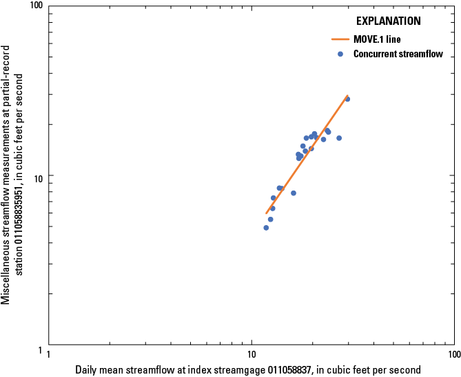
Example of Maintenance of Variance Extension, type 1 (MOVE.1), for U.S. Geological Survey partial-record station Mashpee River at Ashers Path, near Mashpee, Massachusetts (011058835951 and map number 180), with U.S. Geological Survey index streamgage Quashnet River at Waquoit Village, Mass. (011058837 and map number 61). U.S. Geological Survey streamgage and partial-record station are shown in figure 8 and described in table 10.
The streamflow statistics at the index streamgages (Sturtevant and others, 2025) were then entered in the best MOVE.1 relations in table 10 to estimate the statistics at the streamgages and partial-record station. At-site streamflow statistics are provided for the 4 index streamgages, and estimated streamflow statistics based on the MOVE.1 relations are provided for the 3 streamgages and 11 partial-record stations in the Plymouth-Carver-Kingston-Duxbury aquifer system in southeastern Massachusetts and on Cape Cod (Sturtevant and others, 2025).
Groundwater Contributing Areas and Basin Characteristics
Groundwater contributing areas were determined for 4 index streamgages, 3 streamgages with 1 to 4 water years of record, and 11 partial-record stations, as discussed previously. Basin characteristics (aquifer, elevation, physical, land-use, soil, surficial geology, and climate) (table 11) were determined for each of the 18 sites’ groundwater contributing areas (Sturtevant and others, 2025). Aquifer characteristics were determined by using the three previously published groundwater models for the Plymouth-Carver-Kingston-Duxbury aquifer system (Masterson and others, 2009), mid-Cape (LeBlanc and others, 2019), and Lower Cape (Masterson, 2004). Aquifer characteristic determined for the 18 sites included the average depth to the water table; depth to bedrock or the freshwater/saltwater interface; saturated thickness; horizontal hydraulic conductivity; water table slope; maximum, minimum, and mean water table elevations; and other water table elevation characteristics. The other basin characteristics were calculated by using the same GIS coverages as discussed in the previous section “Basin Characteristics” for the mainland regional regression equations.
Table 11.
Basin characteristics determined for the groundwater contributing areas of the 7 U.S. Geological Survey streamgages and 11 partial-record stations in Plymouth-Carver-Kingston-Duxbury aquifer system area in southeastern Massachusetts and on Cape Cod.[NAVD 88, North American Vertical Datum of 1988; SSURGO, Soil Survey Geographic Database; PRISM, Parameter-Elevation Regressions on Independent Slopes Model]
Methods for Estimating Selected Low-Flow Statistics in Southeastern Massachusetts
Development of the Southeastern Regression Equations
The initial regional regression equations for the Plymouth-Carver-Kingston-Duxbury aquifer system in southeastern Massachusetts and Cape Cod (southeastern equations) were developed by using the statistical software TIBCO Spotfire S+ 8.1 for Windows (TIBCO Software, Inc., 2008). The streamflow statistics estimated at the 18 sites (Sturtevant and others, 2025) were tested against the basin characteristics (Sturtevant and others, 2025) to determine potential explanatory variables by following the same procedures (excluding evaluating any hydrologic regions—because the southeastern Massachusetts area is similar hydrogeologically and is a relatively small area) discussed previously for the mainland regional regression equations in the section “Development of Regression Equations.”
Weighting Procedures
For the flow-duration statistics, a weighted procedure was developed to give more weight to sites that had statistics based on more years of record. The seven streamgages were given a weight equivalent to their number of water years of record (table 10). For the partial-record stations, the number of streamflow measurements was then divided by 10 (because most streamgages are measured on average about 8–10 times per year) and then rounded to the nearest whole number to assign a quasi-number of water years (table 10). For example, if 28 streamflow measurements were used in developing the MOVE.1 relation with the index streamgages, then 28 was divided by 10, resulting in 2.8, which would then be rounded up to 3 for the quasi-number of water years for weighting. There is no published guidance on weighting partial-record stations or short-term streamgages with WREG. This weighting procedure was done to ensure that those sites with less information had less weight in the final regression equations.
Final Southeastern Regression Equations
The final southeastern regression equations followed procedures similar to those discussed previously for the mainland regression equations in the section “Final Regression Equations.” Equations for the 99-, 98-, 95-, 90-, 85-, 80-, 75-, 70-, 60-, and 50-percent flow-duration statistics were developed by using weighted least-squares (WLS) regression in the WREG program (Eng and others, 2009). The WLS regression used the number of water years or the equivalent number of water years for the weight (table 10), as discussed in the “Weighting Procedures” section. The regression analyses determined that groundwater contributing area, in square miles and represented by the variable GWCAREA, and percent area of storage (water bodies and wetlands) from the National Land Cover Database (NLCD) of 2016 (Multi-Resolution Land Characteristics Consortium, 2022) in the groundwater contributing area, represented by the variable LC16STOR, were significant explanatory variables in all 10 of the regression equations. The final regression equations for the 10 streamflow statistics (99th- to 50th-percentile flow durations) are listed in table 12.
Table 12.
Summary of southeastern Massachusetts regional regression equations and measures of model accuracy for estimating selected flow-duration streamflow statistics for the Plymouth-Carver-Kingston-Duxbury aquifer system area in southeastern Massachusetts and Cape Cod.[Flow duration is the percentage of time that streamflow was equaled or exceeded. R2, coefficient of determination; MSE, mean square error in log-base 10 logarithm; RMSE, root mean square error, in percent; GWCAREA, groundwater contributing area in square miles; LC16STOR+0.1, percent area of National Land Cover Database 2016 (Multi-Resolution Land Characteristics Consortium, 2022) storage (water bodies and wetlands) plus the value of 0.1 to ensure that there are no zero values; WLS, weighted least-squares regression; WREG, weighted-multiple-linear regression (Eng and others, 2009)]
Groundwater contributing area is expected to be an explanatory variable for these flow-duration equations because groundwater discharge is a large component of streamflow in the groundwater-dominated systems of the Plymouth-Carver-Kingston-Duxbury aquifer system in southeastern Massachusetts and on Cape Cod. Percent area of storage (water bodies and wetlands) of the groundwater contributing area is also likely an explanatory variable because groundwater recharge from water bodies and wetlands is generally less than groundwater recharge on land because evaporation and evapotranspiration is greater for areas of water bodies (ponds) and wetlands, respectively. This is supported by the fact that the groundwater model for the Plymouth-Carver-Kingston-Duxbury aquifer system used recharge rates of 20 inches per year (in/yr) for ponds, 8 in/yr for wetlands, and 27 in/yr for stratified glacial deposits (Masterson and others, 2009, p. 9). Groundwater models for the Sagamore and Monomoy flow lenses (Falmouth to Orleans—west to east) used recharge rates of 16 in/yr for water bodies (ponds), 0.0 in/yr for wetlands, and 24 in/yr for aquifer areas (Walter and Whealan, 2005, pg. 52). Subsequent groundwater models for this same area of Cape Cod by Walter and others (2016) and LeBlanc and others (2019) used the same recharge rates as this study. Walter and Whealan (2005) also noted that other groundwater modeling studies on Cape Cod used recharge rates for wetlands similar to those for water bodies, but in their model, wetland recharge rates of 0.0 in/yr were used and it made little difference in the model results. Groundwater models for the Nauset, Chequesset, Pamet, and Pilgrim lenses (Orleans to Provincetown—south to north) used recharge rates of 14 in/yr for ponds and wetlands and 24 in/yr for the aquifer areas (Masterson, 2004, p. 56).
The RMSE for the 10 regression equations ranged from 33.6 to 62.0 percent (table 12). The low-flow statistics—the 99-, 98-, and 95-percent flow durations—had higher standard errors of the estimate from about 51–62 percent. Generally, the higher flow statistics, 90- to 50-percent flow durations, had lower standard errors of the estimate, between about 47 and 33 percent, respectively. These standard errors of the estimate are consistent with other low-flow studies, as discussed previously in the mainland regional regression equations section “Final Regression Equations.”
Review of areal plots (not shown) of the residuals (differences between streamflow statistics estimated from measured streamflow and those estimated from the regression equations) for selected low-flow durations at the 18 sites in the Plymouth-Carver-Kingston-Duxbury aquifer system in southeastern Massachusetts and on Cape Cod did not indicate any strong regional biases (clear groups of negative or positive residuals). Additionally, plots of the streamflow statistics estimated from measured streamflow (observed data) as functions of the same statistics estimated from the regression equations (predicted data) are presented in figures 10A–E. These plots show no clear bias of the streamflow values generated by regression equations with respect to measured streamflows versus predicted values. However, at lower flows (99-percent flow duration), the range of the data is clearly wider than that for slightly higher low flows (70-percent flow duration). Again, a wider range between observed and predicted data is generally found at the lower flows in all studies that have developed regional regression equations for estimating low-flow statistics. These lower flow statistics (for example, the regression equations for the 99- to 95-percent flow durations) generally have the higher RMSE percentages (table 12).

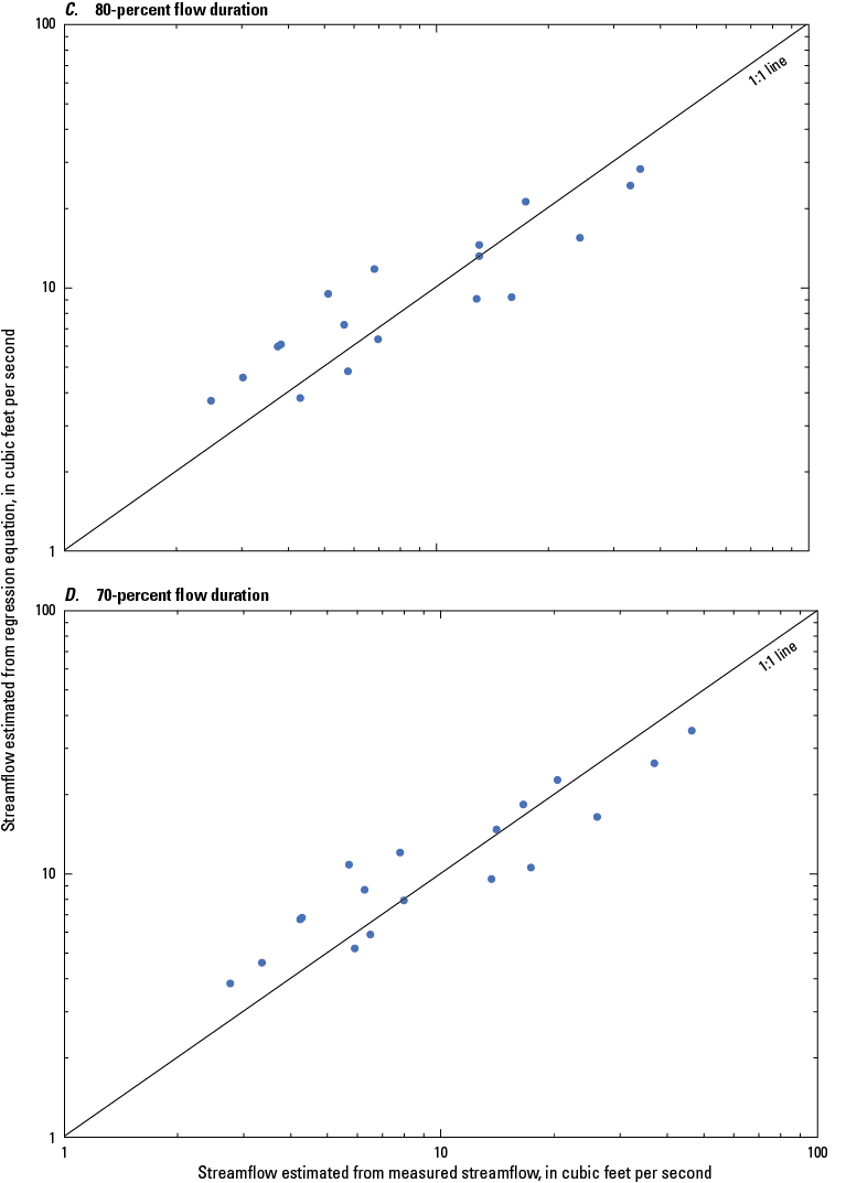
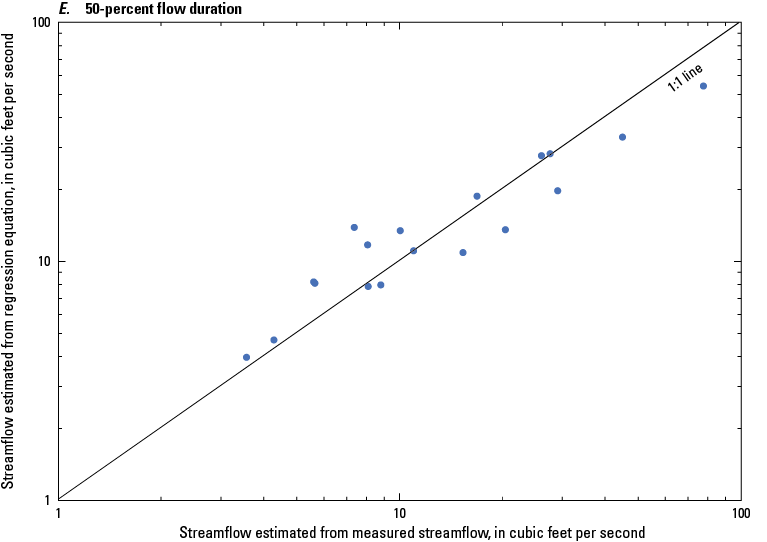
Graphs showing comparisons of the (A) 99-percent, (B) 90-percent, (C) 80-percent, (D) 70-percent, and (E) 50-percent flow durations estimated from measured streamflow and estimated from regression equations for 7 U.S. Geological Survey streamgages and 11 partial-record stations in the Plymouth-Carver-Kingston-Duxbury aquifer system area of southeastern Massachusetts and on Cape Cod.
The lower and upper 90-percent prediction intervals can be calculated by using equations 9–11, discussed in the previous section “Prediction Intervals.” The values of t(α/2, n−p) and U needed for equations 10 and 11 for the 10 southeastern regression equations are presented in table 13. The value of γ2 needed in equation 11 can be calculated by squaring the value of the MSE (base-10 logarithm) in table 13.
Table 13.
Information needed for calculation of the 90-percent prediction intervals for estimates of selected statistics calculated by the southeastern Massachusetts regional regression equations for streamflows in the Plymouth-Carver-Kingston-Duxbury aquifer system area of southeastern Massachusetts and on Cape Cod.[Flow duration is the percentage of time that streamflow was equaled or exceeded. no., number; p, number of parameters, equal to the number of explanatory variables plus 1; t, Student’s t distribution; WLS, weighted least-squares regression; MSE, mean square error; log, base-10 logarithm; RMSE, root mean square error; %, percent; U, covariance matrix for the regression coefficients; GWCAREA, groundwater contributing area in square miles; LC16STOR+0.1, percent area of storage (total wetlands + water bodies) plus the value of 0.1 to ensure there are no zero values (from the National Land Cover Database 2016; Multi-Resolution Land Characteristics Consortium, 2022)]
Limitations of Regression Equations
Use of both the mainland and southeastern regional regression equations is limited by the range of the basin-characteristic data (explanatory variables) used to develop the equations and by the accuracy of the estimates. Additionally, the mainland equations are applicable to all of Massachusetts, excluding the Plymouth-Carver-Kingston-Duxbury aquifer system of southeastern Massachusetts and Cape Cod, and the southeastern equations are only applicable to the Plymouth-Carver-Kingston-Duxbury aquifer system of southeastern Massachusetts and Cape Cod. These equations should not be used for the determination of low-flow statistics at ungaged sites for which the basin characteristics at the ungaged location are outside the range of those characteristics (explanatory variables) used to develop the regression equations. For example, the mainland regression equations would not be applicable for sites on the Merrimack or Connecticut Rivers because those drainage areas are well outside the maximum drainage area used in development of the mainland equations.
The ranges of the basin-characteristic data used as explanatory variables to develop the regression equations for estimating flow durations from the 99th to 50th percentiles, monthly flow durations, median of the monthly means, low-flow frequencies, and other statistics are listed in table 14, and the corresponding accuracies of the estimates calculated by these equations are in tables 8 and 12. The use of these regression equations requires that the basin characteristics be determined in a GIS based on the same datasets (tables 7 and 11; Bent and others, 2025; Sturtevant and others, 2025) that were used to develop the equations outlined in this report.
Table 14.
Range of basin characteristics used as explanatory variables in the regional regression equations for estimating selected streamflow statistics in the mainland area of Massachusetts and in southeastern Massachusetts (Plymouth-Carver-Kingston-Duxbury aquifer system area of southeastern Massachusetts and Cape Cod).[mi2, square mile; SSURGO, Soil Survey Geographic Database (Natural Resources Conservation Service, 2022); %, percent; °F, degree Fahrenheit; NLCD16, National Land Cover Database 2016 (Multi-Resolution Land Characteristics Consortium, 2022)]
The mainland and southeastern equations, which are based on data from streams with minimal to no regulation, give estimates of essentially natural flows for a selected site. They do not give estimates of altered flow for sites where the flow is affected by structures and artificial processes such as dams, surface-water withdrawals, groundwater withdrawals (pumping wells), diversions, or wastewater discharges. To apply the equations to streamflow data for such sites, the user should adjust the estimates for the alterations accordingly.
In southeastern Massachusetts and Cape Cod, groundwater contributing areas and surface-water drainage areas differ appreciably. The southeastern equations include groundwater contributing area, which helps address streamflow differences resulting from the surface-water drainage area and the groundwater contributing area not coinciding at a stream site. This is discussed in detail in this report’s section “Development of Low-Flow Statistics and Basin-Characteristic Datasets for Southeastern Massachusetts and Cape Cod.”
Additionally, the regional regression equations are not applicable to streams with losing stream reaches, which are defined as streams or stream reaches that lose water to the groundwater system (Winter and others, 1998, p. 9–10 and 16–17). Generally, a stream reach is losing where the groundwater table does not intersect the streambed in the channel (the water table is below the streambed) during low-flow periods. Losing stream reaches commonly begin where the stream flows from an area of the basin underlain by till or bedrock to an area underlain by stratified deposits (where hillsides meet river valleys). At such junctures, a stream can lose a substantial amount of water through its streambed.
The accuracies of the regression equations are functions of the quality of the data used to develop the equations. These data include the streamflow data used to estimate the statistics, information about possible unknown flow alterations to the stream upstream from a site, and the measured basin characteristics. Basin characteristics used in the development of the regression equations are limited by the accuracy of the digital data layers available and used at the time (2024) of this study. In the future, the following geospatial data layers of basin characteristics (tables 7 and 11) likely will be more detailed and accurate and at higher resolution:
-
• stream networks from the USGS 3D National Hydrography Program (https://www.usgs.gov/3d-hydrography-program);
-
• elevation from the USGS 3D Elevation Program (https://www.usgs.gov/3d-elevation-program);
-
• land cover and use from the NLCD (https://www.usgs.gov/centers/eros/science/national-land-cover-database);
-
• surficial geology from the Massachusetts Bureau of Geographic Information (MassGIS; https://www.mass.gov/orgs/massgis-bureau-of-geographic-information), Connecticut Department of Energy and Environmental Protection GIS (https://portal.ct.gov/DEEP/GIS-and-Maps/Geographic-Information-Systems), Rhode Island Geographic Information System (https://www.rigis.org/), New Hampshire Geological Survey (https://www.arcgis.com/home/item.html?id=69baea0aea7d4a8593a34f434a01a656), Vermont Center for Geographic Information (https://vcgi.vermont.gov/), and New York State Museum, Geology Geographic Information System (https://www.nysm.nysed.gov/research-collections/geology/gis);
-
• soils from the Natural Resources Conservation Service (https://www.nrcs.usda.gov/conservation-basics/natural-resource-concerns/soil/spatial-data-tools); and
-
• climate data from the PRISM Climate Group, Oregon State University (https://www.prism.oregonstate.edu/).
StreamStats Application and Considerations for Additional Studies
The USGS national StreamStats web-based application (at https://water.usgs.gov/osw/streamstats/; Ries, 2007; Turnipseed and Ries, 2007; Ries and others, 2017; Ries and others, 2024) includes a map-based interface that allows a user to click on the centerline for any stream site to calculate selected streamflow statistics and the prediction intervals from the equations for that ungaged site. The application also provides the user with the basin-characteristic values that were used to calculate the regression equations. The regression equations’ basin-characteristic values for a user-selected stream site are determined by the use of digital map data from ArcGIS (geographic information system software from Esri; https://www.esri.com/). The output includes a map of the drainage-basin boundary (which could be the groundwater contributing area as a substitute), the values of the GIS-measured basin characteristics, the estimated streamflow statistics, and prediction intervals for the estimates. The user can also click on a streamgage and partial-record station symbol and be provided selected streamflow statistics and basin characteristics from a database for that site.
As considerations for additional study, the selected regression equations for streamflow statistics (table 8 and 12), as well as the 90-percent prediction intervals, are expected to be incorporated into the USGS national StreamStats web-based application. The at-site estimates of the selected streamflow statistics at streamgages and partial-record stations could also be put into the StreamStats database for retrieval. Another consideration is that new or more detailed basin characteristics that were not available for this study (2024) may be available in the future and could be tested as potential explanatory variables. These digital data layers likely would improve the accuracy of the measured basin characteristics used as explanatory variables in either or both the mainland and southeastern regional regression equations to estimate selected low-flow statistics, but only after re-examination of the regression equations. Additional streamflow data in the Plymouth-Carver-Kingston-Duxbury aquifer system of southeastern Massachusetts and Cape Cod would likely improve the streamflow statistics estimated for streamgages and partial-record stations, thus improving the southeastern Massachusetts regional regression equations developed.
Summary and Conclusions
The U.S. Geological Survey, in cooperation with the Massachusetts Department of Conservation and Recreation, Office of Water Resources, developed regional regression equations for estimating selected natural to near natural—with minimal to no regulations—streamflows for specific low-flow statistics durations, low-flow frequencies, and monthly and annual statistics at ungaged stream sites for two areas of Massachusetts. Selected at-site streamflow statistics are also provided for 174 long-term streamgages in and near Massachusetts. The regional regression equations for estimating selected streamflow statistics and the at-site statistics estimated may be used by Federal, State, and local water managers in addressing water issues in and near Massachusetts.
Streamgages with minimal to no regulation were selected for the “mainland” regional regression analyses (excluding the Plymouth-Carver-Kingston-Duxbury aquifer system in southeastern Massachusetts and Cape Cod). Upstream water-use and wastewater discharge data and hydrologic disturbance index data were also evaluated in the selection process. Since a large number of streamgages in Massachusetts are regulated, streamgages within about 25 miles of the State border were also evaluated. Streamgages used in previous low-flow regression analyses studies generally were selected. This process resulted in 81 streamgages in and near Massachusetts being selected for the mainland regional regression analyses.
All 174 streamgages were evaluated for any possible significant trends in the annual 7-day low flows over the past 30-, 50-, 70-, and 90-year periods ending in climatic year 2019. No clear trends were found in the annual 7-day low flows during the four periods: 1990–2019, 1970–2019, 1950–2019, and 1930–2019. Several streamgages showed trends, but not always over all four periods and also not always in the same direction (increasing or decreasing). Only the Deerfield River at Charlemont, Massachusetts (01168500), streamgage had the same significant trend—increasing—over all four periods evaluated. Flows at this streamgage are affected by hydropower generation.
Basin characteristics (hydrography, elevation, physical, land-use, soil, surficial geology, and climate) were determined by using GIS data layers available for Massachusetts and the surrounding States for the 174 streamgages. Streamflow variability index (SVI), which is a general measure of groundwater contribution and surface-water storage, was determined by using flow durations at streamgages in southern New England and eastern New York. To improve the SVI map for the study, an equation was developed between the SVIs for flow durations from the 95th to 50th percentiles and the SVIs for flow durations from the 95th to 5th percentiles by using 248 streamgages with 8 or more water years of record. This equation was then used to estimate the SVIs for flow durations from the 95th to 5th percentiles at partial-record stations with published flow durations from the 95th to 50th percentiles. The SVI map for southern New England and eastern New York included data from 276 streamgages with 8 or more water years of record, 102 streamgages with less than 8 water years of record, and 286 partial-record stations. The SVI map was developing by using kriging a geostatistical technique. These basin characteristics, including SVI, were tested as potential explanatory variables for the mainland regional regression equations for the selected streamflow statistics.
The mainland regional regression equations were developed to estimate 27 streamflow statistics: 99-, 98-, 95-, 90-, 85-, 80-, 75-, 70-, 60-, and 50-percent flow durations; monthly June, July, August, and September 90- and 50-percent flow durations; February, June, and August median of the monthly means; harmonic mean; and medians of the following annual frequency statistics: 7-day; 7-day, 2-year; 7-day, 10-year; 30-day, 2-year; and 30-day, 10-year. A number of additional streamflow statistics, for which regression equations were not developed, also were estimated for the long-term streamgages in and near Massachusetts.
The mainland regression equations used to estimate the selected streamflow statistics were developed by relating the statistics to basin characteristics at the 81 streamgages in and near Massachusetts. The regression analyses were completed by using the weighted least-squares (non-frequency statistics—flow durations, medians, and means) or the generalized least-squares techniques (frequency statistics—30-day, 2-year and 30-day, 10-year) in the weighted-multiple-linear regression program for the 27 statistics. The equations for frequency statistics 7-day, 2-year and 7-day, 10-year required weighted left-censored regression analyses because one and five streamgages, respectively, had zero flow for those statistics. The regression analyses determined that four basin characteristics—drainage area, percent area of the combined hydrologic soil groups A and B, SVI, and annual mean temperature—were the only significant explanatory variables for the different regression equations. Drainage area was an explanatory variable in all equations, combined hydrologic soil groups A and B was generally a variable in the more moderate flow statistics, SVI was generally a variable in the lower flow statistics, and annual mean temperature was a variable in only one equation—the median of February monthly mean flows. The standard error of the estimate for the 27 regression equations ranged from about 17 to 131 percent. The lower flow statistic equations had the higher standard errors of the estimate, and the standard errors of the estimate decreased as the flows increased. The 90-percent prediction intervals for the 27 streamflow statistics were also calculated.
Regional regression equations were also developed for the Plymouth-Carver-Kingston-Duxbury aquifer system of southeastern Massachusetts and Cape Cod (“southeastern” equations) because this area of the State is hydrologically different in that surface-water drainage area and groundwater contributing areas do not always coincide. Streamflow statistics were computed at 4 streamgages with 14 or more water years of record and estimated at 3 streamgages with less than 4 water years of record and at 11 partial-record stations. Streamflow statistics estimated at the 3 streamgages and 11 partial-record stations were completed by using the Maintenance of Variance Extension, type 1, record-extension technique, which determines an equation relating streamflow data (daily mean discharge and measurements, respectively) at the 14 sites to concurrent daily mean discharge at nearby index streamgages. The low-flow statistics at the most representative index streamgage (highest correlation coefficient or most linear relation to each of the 11 sites) are then entered into the Maintenance of Variance Extension, type 1, equation to estimate the low-flow statistics at each of the 11 sites. Some of streamgages and partial-record stations used in this analysis have occasional minor regulations—mainly for cranberry bog maintenance, irrigation, and harvesting and some water-supply withdrawals.
To develop the southeastern regional regression equations to estimate low-flow statistics, the groundwater contributing area of each of the 18 sites was determined. The groundwater contributing areas were determined by using three previously published groundwater models and using water-particle-tracking simulations. Basin characteristics (aquifer, elevation, physical, land-use, soil, surficial geology, and climate) were then calculated by using the groundwater contributing areas. Additionally, aquifer characteristics such as the mean depth to the water table, water table slope, saturated thickness, horizontal hydraulic conductivity, and transmissivity were also calculated for groundwater contributing areas. These basin characteristics were tested as potential explanatory variables for the southeastern regional regression equations for the selected streamflow statistics.
The southeastern regional regression analyses were done by using weighted least-squares regression in the weighted-multiple-linear regression program for the 10 flow durations from the 99th to 50th percentiles. The regression analyses determined that groundwater contributing area and percent area of storage (water bodies and wetlands) were the only significant explanatory variables for the regression equations. The standard error of the estimate for the 10 regression equations ranged from about 33 to 62 percent. The lower flow statistics had the higher standard errors of the estimate, and the standard errors of the estimate decreased as flows increased.
The mainland regional regression equations developed for this study are based on data from streams with little to no regulation and provide an estimate of the natural flows for a selected ungaged site. They do not estimate flows for regulated sites with dams, surface-water withdrawals, groundwater withdrawals (pumping wells), diversions, and wastewater discharges. If the equations are used to estimate streamflow statistics for regulated sites, the user should adjust the flow estimates to account for the known regulations. The southeastern regional regression equations include some sites with occasional minor regulations but, overall, represent fairly natural streamflows. If the equations are used to estimate streamflow statistics for regulated sites, the user should adjust the flow estimates for the known regulations. Both the mainland and southeastern regional regression equations are expected to be incorporated into the U.S. Geological Survey StreamStats web-based application (https://streamstats.usgs.gov/ss/) to allow users to locate a stream site on a map and automatically compute the needed basin characteristics and compute the estimated low-flow statistics and associated prediction intervals.
References Cited
Ahearn, E.A., 2008, Flow durations, low-flow frequencies, and monthly median flows for selected streams in Connecticut through 2005: U.S. Geological Survey Scientific Investigations Report 2007–5270, 33 p., accessed March 3, 2023, at https://pubs.usgs.gov/sir/2007/5270/.
Ahearn, E.A., 2010, Regional regression equations to estimate flow-duration statistics at ungaged stream sites in Connecticut: U.S. Geological Survey Scientific Investigations Report 2010–5052, 45 p. [Also available at https://doi.org/10.3133/sir20105052.]
Ahearn, E.A., and Hodgkins, G.A., 2020, Estimating flood magnitude and frequency on streams and rivers in Connecticut, based on data through water year 2015: U.S. Geological Survey Scientific Investigations Report 2020–5054, 42 p., accessed October 6, 2023, at https://doi.org/10.3133/sir20205054.
Ahearn, E.A., Ries, K.G., III, and Steeves, P.A., 2006, Streamstats—U.S. Geological Survey web application for streamflow statistics for Connecticut: U.S. Geological Survey Fact Sheet 2006–3129, 4 p. [Also available at https://doi.org/10.3133/fs20063129.]
Archfield, S.A., Vogel, R.M., Steeves, P.A., Brandt, S.L., Weiskel, P.K., and Garabedian, S.P., 2010, The Massachusetts Sustainable-Yield Estimator—A decision support tool to assess water availability at ungaged stream locations in Massachusetts: U.S. Geological Survey Scientific Investigations Report 2009–5227, 41 p., plus CD–ROM. [Also available at https://doi.org/10.3133/sir20095227.]
Armstrong, D.S., Parker, G.W., and Richards, T.A., 2008, Characteristics and classification of least altered streamflows in Massachusetts: U.S. Geological Survey Scientific Investigations Report 2007–5291, 113 p., plus CD–ROM. [Also available at https://doi.org/10.3133/sir20075291.]
Barbaro, J.R., Masterson, J.P., and LeBlanc, D.R., 2014, Science for the stewardship of the groundwater resources of Cape Cod, Massachusetts: U.S. Geological Survey Fact Sheet 2014–3067, 6 p. [Also available at https://doi.org/10.3133/fs20143067.]
Barlow, P.M., McHugh, A.R., Kiang, J.E., Zhai, T., Hummel, P., Duda, P., and Hinz, S., 2022, U.S. Geological Survey Hydrologic Toolbox—A graphical and mapping interface for analysis of hydrologic data: U.S. Geological Survey Techniques and Methods, book 4, chap. D3, 23 p., accessed December 3, 2023, at https://doi.org/10.3133/tm4D3.
Bent, G.C., 1995, Streamflow, groundwater recharge and discharge, and characteristics of surficial deposits in Buzzards Bay Basin, southeastern Massachusetts: U.S. Geological Survey Water-Resources Investigations Report 95–4234, 56 p. [Also available at https://doi.org/10.3133/wri954234.]
Bent, G.C., 1999, Streamflow, base flow, and ground-water recharge in the Housatonic River Basin, western Massachusetts and parts of eastern New York and northwestern Connecticut: U.S. Geological Survey Water-Resources Investigations Report 98–4232, 68 p. [Also available at https://doi.org/10.3133/wri984232.]
Bent, G.C., Ahearn, E.A., Fair, J.H., Mazo, C.F., and Harrington, L.E., 2025, Low-flow statistic equations and supplementary data for Massachusetts: U.S. Geological Survey data release, https://doi.org/10.5066/P13AI5EP.
Bent, G.C., and Archfield, S.A., 2002, A logistic regression equation for estimating the probability of a stream flowing perennially in Massachusetts: U.S. Geological Survey Water-Resources Investigations Report 02–4043, 45 p. [Also available at https://doi.org/10.3133/wri024043.]
Bent, G.C., and Steeves, P.A., 2006, A revised logistic regression equation and an automated procedure for mapping the probability of a stream flowing perennially in Massachusetts: U.S. Geological Survey Scientific Investigations Report 2006–5031, 107 p. [Also available at https://doi.org/10.3133/sir20065031.]
Bent, G.C., and Waite, A.M., 2013, Equations for estimating bankfull channel geometry and discharge for streams in Massachusetts: U.S. Geological Survey Scientific Investigations Report 2013–5155, 62 p. [Also available at https://doi.org/10.3133/sir20135155.]
Bent, G.C., Steeves, P.A., and Waite, A.M., 2014, Equations for estimating selected streamflow statistics in Rhode Island: U.S. Geological Survey Scientific Investigations Report 2014–5010, 65 p. [Also available at https://doi.org/10.3133/sir20145010.]
Bisese, J.A., 1995, Methods for estimating the magnitude and frequency of peak discharges of rural, unregulated streams in Virginia: U.S. Geological Survey Water-Resources Investigations Report 94–4148, 70 p., 1 pl., scale 1:500,000. [Also available at https://doi.org/10.3133/wri944148.]
Carlson, C.S., 2025, MODPATH6 datasets using MODFLOW and SEAWAT input for development of groundwater contributing areas for estimating low-flow statistics for the Plymouth-Carver aquifer area and Cape Cod, Massachusetts: U.S. Geological Survey data release, https://doi.org/10.5066/P142FWRJ.
Carlson, C.S., Masterson, J.P., Walter, D.A., and Barbaro, J.R., 2017, Simulated groundwater-contributing areas to selected streams, ponds, coastal water bodies, and production wells, Plymouth-Carver region and Cape Cod, Massachusetts: U.S. Geological Survey data release, accessed January 23, 2024, at https://doi.org/10.5066/F7V69H2Z.
Cervione, M.A., Jr., Richardson, A.R., and Weiss, L.A., 1993, Low-flow characteristics of selected streams in Rhode Island: U.S. Geological Survey Water-Resources Investigations Report 93–4046, 16 p. [Also available at https://doi.org/10.3133/wri934046.]
Choquette, A.F., 1988, Regionalization of peak discharges for streams in Kentucky: U.S. Geological Survey Water Resources Investigations Report 87–4209, 105 p., 1 pl., scale 1:500,000. [Also available at https://doi.org/10.3133/wri874209.]
Cohn, T.A., 1988, Adjusted maximum likelihood estimation of the moments of lognormal populations from type I censored data: U.S. Geological Survey Open-File Report 88–350, 34 p. [Also available at https://doi.org/10.3133/ofr88350.]
Cohn, T.A., and Lins, H.F., 2005, Nature’s style—Naturally trendy: Geophysical Research Letters, v. 32, no. 23, 5 p., accessed August 30, 2017, at https://doi.org/10.1029/2005GL024476.
Connecticut Department of Energy and Environmental Protection, 2022, Surficial materials set: Connecticut Department of Energy and Environmental Protection Geographic Information Systems Open Data website data layer, accessed May 23, 2022, at https://deepmaps.ct.gov/maps/608054746f2d4577a5683c8f9d190d8f/about.
DelSanto, A., Bhuiyan, M.A.E., Andreadis, K.M., and Palmer, R.N., 2023, Low-flow (7-day, 10-year) classical statistical and improved machine learning estimation methodologies: Water, v. 15, no. 15, article 2813, 31 p., accessed May 23, 2024, at https://www.mdpi.com/2073-4441/15/15/2813.
Denny, C.S., 1982, Geomorphology of New England: U.S. Geological Survey Professional Paper 1208, 18 p., 1 pl. [Also available at https://doi.org/10.3133/pp1208.]
Dudley, R.W., Hirsch, R.M., Archfield, S.A., Blum, A.G., and Renard, B., 2020, Journal of Hydrology: v. 580, article 124254, 13 p., accessed June 8, 2023, at https://doi.org/10.1016/j.jhydrol.2019.124254.
Eash, D.A., and Barnes, K.K., 2012, Methods for estimating low-flow frequency statistics and harmonic mean flows for streams in Iowa (ver. 1.1, November 2017): U.S. Geological Survey Scientific Investigations Report 2012–5171, 99 p., accessed May 21, 2023, at https://pubs.usgs.gov/sir/2012/5171/.
Eng, K., Chen, Y.-Y., and Kiang, J.E., 2009, User’s guide to the weighted-multiple-linear regression program (WREG version 1.0): U.S. Geological Survey Techniques and Methods, book 4, chap. A8, 21 p. [Also available at https://doi.org/10.3133/tm4A8.]
Esri, 2022, USA SSURGO—Soil hydrologic group: Esri ArcGIS Hub web page, accessed July 28, 2022, at https://hub.arcgis.com/maps/uneplive:usa-ssurgo-soil-hydrologic-group/about.
Esri, 2023a, How kriging works: Esri web page, accessed March 31, 2023, at https://pro.arcgis.com/en/pro-app/latest/tool-reference/spatial-analyst/how-kriging-works.htm.
Esri, 2023b, Kriging (3D analyst): Esri web page, accessed March 31, 2023, at https://pro.arcgis.com/en/pro-app/latest/tool-reference/3d-analyst/kriging.htm.
Esri, 2023c, Understanding interpolation analysis: Esri web page accessed March 31, 2023, at https://pro.arcgis.com/en/pro-app/latest/tool-reference/3d-analyst/understanding-interpolation-analysis.htm.
Falcone, J., 2011, GAGES–II, geospatial attributes of gages for evaluating streamflow: U.S. Geological Survey data release, accessed July 21, 2021, at https://www.sciencebase.gov/catalog/item/521e4686e4b051c878dc35d0.
Farmer, W.H., 2023, WREG—Weighted least squares regression for streamflow frequency statistics: U.S. Geological Survey software release, accessed March 3, 2023, at https://doi.org/10.5066/P9ZCGLI1.
Farmer, W.H., Kiang, J.E., Feaster, T.D., and Eng, K., 2019, Regionalization of surface-water statistics using multiple linear regression: U.S. Geological Survey Techniques and Methods, book 4, chap. A12, 40 p. [Also available at https://doi.org/10.3133/tm4A12.]
Feaster, T.D., Kolb, K.R., Painter, J.A., and Clark, J.M., 2020, Methods for estimating selected low-flow frequency statistics and mean annual flow for ungaged locations on streams in Alabama (ver. 1.2, November 20, 2020): U.S. Geological Survey Scientific Investigations Report 2020–5099, 21 p. [Also available at https://doi.org/10.3133/sir20205099.]
Fennessey, N., and Vogel, R.M., 1990, Regional flow-duration curves for ungauged sites in Massachusetts: Journal of Water Resources Planning and Management, v. 116, no. 4, p. 530–549. [Also available at https://doi.org/10.1061/(ASCE)0733-9496(1990)116:4(530).]
Flynn, R.H., 2003a, A stream-gaging network analysis for the 7-day, 10-year annual low flow in New Hampshire Streams: U.S. Geological Survey Water-Resources Investigations Report 03–4023, 31 p., accessed August 18, 2025, at https://pubs.usgs.gov/wri/wrir03-4023/.
Flynn, R.H., 2003b, Development of regression equations to estimate flow durations and low-frequency statistics in New Hampshire streams: U.S. Geological Survey Water Resources Investigations Report 02–4298, 66 p., accessed August 18, 2025, at https://pubs.usgs.gov/wri/wri02-4298/.
Friel, E.A., Embree, W.N., Jack, A.R., and Atkins, J.T., Jr., 1989, Low-flow characteristics of streams in West Virginia: U.S. Geological Survey Water-Resources Investigations Report 88–4072, 34 p. [Also available at https://doi.org/10.3133/wri884072.]
Gotvald, A.J., 2017, Methods for estimating selected low-flow frequency statistics and mean annual flow for ungaged locations on streams in North Georgia: U.S. Geological Survey Scientific Investigations Report 2017–5001, 25 p. [Also available at https://doi.org/10.3133/sir20175001.]
Granato, G.E., 2009, Computer programs for obtaining and analyzing daily mean streamflow data from the U.S. Geological Survey National Water Information System Web Site: U.S. Geological Survey Open-File Report 2008–1362, 123 p., on CD–ROM. [Also available at https://doi.org/10.3133/ofr20081362].
Hamed, K.H., 2008, Trend detection in hydrologic data—The Mann-Kendall trend test under the scaling hypothesis: Journal of Hydrology, v. 349, nos. 3–4, p. 350–363. [Also available at https://doi.org/10.1016/j.jhydrol.2007.11.009.]
Hamed, K.H., and Ramachandra Rao, A., 1998, A modified Mann-Kendall trend test for autocorrelated data: Journal of Hydrology, v. 204, nos. 1–4, p. 182–196. [Also available at https://doi.org/10.1016/S0022-1694(97)00125-X.]
Hansen, B.P., and Lapham, W.W., 1992, Geohydrology and simulated ground-water flow, Plymouth-Carver Aquifer, southeastern Massachusetts: U.S. Geological Survey Water-Resources Investigations Report 90–4204, 69 p. [Also available at https://pubs.usgs.gov/wri/wri904204/.]
Harvard Forest, 2020, Land sector report—A technical report of the Massachusetts 2050 decarbonization roadmap study, December 2020: Commonwealth of Massachusetts, prepared by Harvard Forest, 62 p., accessed January 25, 2024, at https://www.mass.gov/doc/land-sector-technical-report/download.
Helsel, D.R., and Hirsch, R.M., 2002, Statistical methods in water resources: U.S. Geological Survey Techniques of Water Resources Investigations, book 4, chap. A3, 522 p. [Also available at https://doi.org/10.3133/tm4A3.]
Hirsch, R.M., 1982, A comparison of four streamflow record extension techniques: Water Resources Research, v. 18, no. 4, p. 1081–1088. [Also available at https://doi.org/10.1029/WR018i004p01081.]
Hodgkins, G.A., and Dudley, R.W., 2011, Historical summer base flow and stormflow trends for New England rivers: Water Resources Research, v. 47, no. 7, article W07528, 16 p. [Also available at https://doi.org/10.1029/2010WR009109.]
Hodgkins, G.A., Whitfield, P.H., Burn, D.H., Hannaford, J., Renard, B., Stahl, K., Fleig, A.K., Madsen, H., Mediero, L., Korhonen, J., Murphy, C., and Wilson, D., 2017, Climate-driven variability in the occurrence of major floods across North America and Europe: Journal of Hydrology, v. 552, p. 704–717. [Also available at https://doi.org/10.1016/j.jhydrol.2017.07.027.]
Khaliq, M.N., Ouarda, T.B.M.J., and Gachon, P., 2009, Identification of temporal trends in annual and seasonal low flows occurring in Canadian rivers—The effect of short- and long-term persistence: Journal of Hydrology, v. 369, nos. 1–2, p. 183–197. [Also available at https://doi.org/10.1016/j.jhydrol.2009.02.045.]
Kliever, J.D., 1996, Low-flow characteristics of selected streams in northern Rhode Island: U.S. Geological Survey Water-Resources Investigations Report 95–4299, 11 p. [Also available at https://doi.org/10.3133/wri954299.]
Koltun, G.F., and Kula, S.P., 2013, Methods for estimating selected low-flow statistics and development of annual flow-duration statistics for Ohio: U.S. Geological Survey Scientific Investigations Report 2012–5138, 195 p. [Also available at https://doi.org/10.3133/sir20125138.]
Koltun, G.F., and Roberts, J.W., 1990, Techniques for estimating flood-peak discharges of rural, unregulated stream in Ohio: U.S. Geological Survey Water-Resources Investigations Report 89–4126, 68 p., 1 pl. [Also available at https://doi.org/10.3133/wri894126.]
Koltun, G.F., and Schwartz, R.R., 1987, Multiple-regression equations for estimating low flows at ungaged stream sites in Ohio: U.S. Geological Survey Water-Resources Investigations Report 86–4354, 39 p., 6 pls. [Also available at https://doi.org/10.3133/wri864354.]
Koltun, G.F., and Whitehead, M.T., 2002, Techniques for estimating selected streamflow characteristics of rural unregulated streams in Ohio: U.S. Geological Survey Water Resources Investigations Report 02–4068, 50 p. [Also available at https://doi.org/10.3133/wri024068.]
Koutsoyiannis, D., and Montanari, A., 2007, Statistical analysis of hydroclimatic time series—Uncertainty and insights: Water Resources Research, v. 43, no. 5. [Also available at https://doi.org/10.1029/2006WR005592.]
Kroll, C.N., and Stedinger, J.R., 1999, Development of regional regression relationships with censored data: Water Resources Research, v. 35, no. 3, p. 775–784. [Also available at https://doi.org/10.1029/98WR02743.]
Kumar, S., Merwade, V., Kam, J., and Thurner, K., 2009, Streamflow trends in Indiana—Effects of long term persistence, precipitation and subsurface drains: Journal of Hydrology, v. 374, nos. 1–2, p. 171–183. [Also available at https://doi.org/10.1016/j.jhydrol.2009.06.012.]
LeBlanc, D.R., McCobb, T.D., and Barbaro, J.R., 2019, Simulated water-table and pond-level responses to proposed public water-supply withdrawals in the Hyannis Ponds Wildlife Management Area, Barnstable, Massachusetts: U.S. Geological Survey Scientific Investigations Report 2019–5121, 32 p., accessed December 18, 2023, at https://doi.org/10.3133/sir20195121.
Levin, S.B., and Granato, G.E., 2018, Methods used to estimate daily streamflow and water availability in the Massachusetts Sustainable-Yield Estimator version 2.0: U.S. Geological Survey Scientific Investigations Report 2018–5146, 16 p., accessed December 13, 2022, at https://doi.org/10.3133/sir20185146.
Lins, H.F., and Slack, J.R., 2005, Seasonal and regional characteristics of U.S. streamflow trends in the United States from 1940 to 1999: Physical Geography, v. 26, no. 6, p. 489–501. [Also available at https://doi.org/10.2747/0272-3646.26.6.489.]
Lorenz, D.L., 2015, censReg—Censored data regression in USGS-R/smwrQW: U.S. Geological Survey documentation, accessed June 30, 2024, at https://rdrr.io/github/USGS-R/smwrQW/man/censReg.html.
Ludwig, A.H., and Tasker, G.D., 1993, Regionalization of low-flow characteristics of Arkansas streams: U.S. Geological Survey Water-Resources Investigations Report 93–4013, 32 p. [Also available at https://doi.org/10.3133/wri934013.]
Lumia, R., 1991, Regionalization of flood discharges for rural, unregulated streams in New York, excluding Long Island: U.S. Geological Survey Water-Resources Investigations Report 90–4197, 119 p., 2 pls., scale 1:500,000. [Also available at https://doi.org/10.3133/wri904197.]
Martin, G.R., and Arihood, L.D., 2010, Methods for estimating selected low-flow frequency statistics for unregulated streams in Kentucky: U.S. Geological Survey Scientific Investigations Report 2010–5217, 83 p., accessed February 24, 2023, at https://pubs.usgs.gov/sir/2010/5217/.
Martin, G.R., and Ruhl, K.J., 1993, Regionalization of harmonic-mean streamflows in Kentucky: U.S. Geological Survey Water-Resources Investigations Report 92–4173, 47 p., 1 pl., scale 1:500,000. [Also available at https://doi.org/10.3133/wri924173.]
Massachusetts Bureau of Geographic Information, 2022, USGS 1:24,000 surficial geology: Massachusetts Bureau of Geographic Information database, accessed May 23, 2022, at https://www.mass.gov/info-details/massgis-data-usgs-124000-surficial-geology.
Massachusetts Department of Conservation and Recreation, Office of Water Resources, 2008, 2008 index streamflows for Massachusetts: Massachusetts Water Resources Commission, [variously paged; 386 p.], accessed January 8, 2023, at https://www.mass.gov/doc/2008-index-streamflows-in-massachusetts/download.
Massachusetts Department of Environmental Protection, 2023, Water management act program: Commonwealth of Massachusetts web page, accessed December 3, 2023, at https://www.mass.gov/water-management-act-program.
Massachusetts Department of Environmental Protection, 2024a, 310 code of Massachusetts regulations 10.00—Wetlands protection act regulations: Commonwealth of Massachusetts web page, accessed June 30, 2024, at https://www.mass.gov/regulations/310-CMR-1000-wetlands-protection-act-regulations.
Massachusetts Department of Environmental Protection, 2024b, Water management act permits issued since 2015: Commonwealth of Massachusetts web page, accessed May 23, 2024, at https://www.mass.gov/guides/water-management-act-permits-and-decisions.
Massachusetts Executive Office of Energy and Environmental Affairs and Massachusetts Emergency Management Agency, 2023, Massachusetts drought management plan—Preparedness and response: Massachusetts Executive Office of Energy and Environmental Affairs, 115 p., accessed February 24, 2024, at https://www.mass.gov/info-details/drought-management-plan.
Massachusetts Water Resources Commission, 2023, Results of a stressed basin report in Massachusetts: Commonwealth of Massachusetts web page, accessed January 8, 2023, at https://www.mass.gov/service-details/results-of-the-stressed-basins-in-massachusetts-report.
Massachusetts Water Resources Commission, 2024, Drought status—Drought Management Task Force: Commonwealth of Massachusetts web page, accessed February 24, 2024, at https://www.mass.gov/info-details/drought-status.
Masterson, J.P., 2004, Simulated interaction between freshwater and saltwater and effects of ground-water pumping and sea-level change, Lower Cape Cod aquifer system, Massachusetts: U.S. Geological Survey Scientific Investigations Report 2004–5014, 78 p. [Also available at https://doi.org/10.3133/sir20045014.]
Masterson, J.P., Carlson, C.S., and Walter, D.A., 2009, Hydrogeology and simulation of groundwater flow in the Plymouth-Carver-Kingston-Duxbury aquifer system, southeastern Massachusetts: U.S. Geological Survey Scientific Investigations Report 2009–5063, 110 p. [Also available at https://doi.org/10.3133/sir20095063.]
Masterson, J.P., and Walter, D.A., 2009, Hydrogeology and groundwater resources of the coastal aquifers of southeastern Massachusetts: U.S. Geological Survey Circular 1338, 16 p. [Also available at https://doi.org/10.3133/cir1338.]
McCabe, G.J., and Wolock, D.M., 2002, A step increase in streamflow in the conterminous United States: Geophysical Research Letters, v. 29, no. 24, p. 2185–2189. [Also available at https://doi.org/10.1029/2002GL015999.]
Milly, P.C.D., Betancourt, J., Falkenmark, M., Hirsch, R.M., Kundzewicz, Z.W., Lettenmaier, D.P., and Stouffer, R.J., 2008, Stationarity is dead—Whither water management?: Science, v. 319, no. 5863, p. 573–574. [Also available at https://doi.org/10.1126/science.1151915.]
Multi-Resolution Land Characteristics Consortium, 2022, National land cover database (NLCD) 2016 land cover (CONUS): Multi-Resolution Land Characteristics Consortium website, accessed April 2, 2022, at https://www.mrlc.gov/data.
Natural Resources Conservation Service, 2022, Soil survey geographic database: Natural Resources Conservation Service database, accessed June 8, 2022, at https://www.nrcs.usda.gov/resources/data-and-reports/soil-survey-geographic-database-ssurgo.
New Hampshire Geological Survey, 2022, New Hampshire Geological Survey interactive publication viewer website, accessed May 23, 2022, at https://www.arcgis.com/home/item.html?id=69baea0aea7d4a8593a34f434a01a656.
New York State Museum, 2022, Geology—Geographic information system (GIS): New York State Museum web page accessed May 23, 2022, at https://nysm.nysed.gov/research-collections/geology/gis.
Pollock, D.W., 2012, User guide for MODPATH version 6—A particle-tracking model for MODFLOW: U.S. Geological Survey Techniques and Methods, book 6, chap. A41, 58 p., accessed February 24, 2024, at https://pubs.usgs.gov/publication/tm6A41.
PRISM Climate Group, 2021, Parameter-elevation regressions on independent slopes model climate mapping system: PRISM Climate Group dataset, accessed June 8, 2021, at https://www.prism.oregonstate.edu/.
Randall, A.D., and Freehafer, D.A., 2017, Estimation of low-flow statistics at ungaged sites on streams in the Lower Hudson River Basin, New York, from data in geographic information systems: U.S. Geological Survey Scientific Investigations Report 2017–5019, 42 p., accessed June 30, 2022, at https://doi.org/10.3133/sir20175019.
Rhode Island Geographic Information System, 2022, Glacial deposits: Rhode Island Geographic Information System dataset accessed May 23, 2022, at https://www.rigis.org/datasets/f0c82668092240e0abc0128a89b07137_0/explore?location=41.577216%2C-71.498024%2C9.93.
Ries, K.G., III, 1990, Estimating surface-water runoff to Narragansett Bay, Rhode Island and Massachusetts: U.S. Geological Survey Water-Resources Investigations Report 89–4164, 44 p., 1 pl., scale 1:125,000. [Also available at https://doi.org/10.3133/wri894164.]
Ries, K.G., III, 1994a, Development and application of generalized least-squares regression models to estimate low-flow duration discharges in Massachusetts: U.S. Geological Survey Water-Resources Investigations Report 94–4155, 33 p. [Also available at https://doi.org/10.3133/wri944155.]
Ries, K.G., III, 1994b, Estimation of low-flow duration discharges in Massachusetts: U.S. Geological Survey Water-Supply Paper 2418, 50 p. [Also available at https://doi.org/10.3133/wsp2418.]
Ries, K.G., III, 1997, August median streamflows in Massachusetts: U.S. Geological Survey Water-Resources Investigations Report 97–4190, 27 p. [Also available at https://doi.org/10.3133/wri974190.]
Ries, K.G., III, 1999, Streamflow measurements, basin characteristics, and streamflow statistics for low-flow partial-record stations operated in Massachusetts from 1989 through 1996: U.S. Geological Survey Water-Resources Investigations Report 99–4006, 162 p. [Also available at https://doi.org/10.3133/wri994006.]
Ries, K.G., III, 2007, The national streamflow statistics program—A computer program for estimating streamflow statistics for ungaged sites: U.S. Geological Survey Techniques and Methods, book 4, chap. A6, 37 p. [Also available at https://doi.org/10.3133/tm4A6.]
Ries, K.G., III, and Friesz, P.J., 2000, Methods for estimating low-flow statistics for Massachusetts streams: U.S. Geological Water-Resources Investigations 00–4135, 81 p. [Also available at https://doi.org/10.3133/wri004135.]
Ries, K.G., III, Newson J.K., Smith, M.J., Guthrie, J.D., Steeves, P.A., Haluska, T.L., Kolb, K.R., Thompson, R.F., Santoro, R.D., and Vraga, H.W., 2017, StreamStats, version 4: U.S. Geological Survey Fact Sheet 2017–3046, 4 p. [Also available at https://doi.org/10.3133/fs20173046.]
Ries, K.J., III, and Steeves, P.A., Freeman, A., and Singh, R., 2000, Obtaining streamflow statistics for Massachusetts streams on the World Wide Web: U.S. Geological Survey Fact Sheet FS–104–00, 4 p. [Also available at https://doi.org/10.3133/fs10400.]
Ries, K.G., III, Steeves, P.A., and McCarthy, P., 2024, StreamStats—A quarter century of delivering web-based geospatial and hydrologic information to the public, and lessons learned: U.S. Geological Survey Circular 1514, 40 p. [Also available at https://doi.org/10.3133/cir1514.]
Riggs, H.C., 1972, Low-flow investigations: U.S. Geological Survey Techniques of Water-Resources Investigations, book 4, chap. B1, 18 p. [Also available at https://doi.org/10.3133/twri04B1.]
Risley, J.C., 1994, Estimating the magnitude and frequency of low flows of streams in Massachusetts: U.S. Geological Survey Water-Resources Investigations Report 94–4100, 29 p. [Also available at https://doi.org/10.3133/wri944100.]
Rossman, L.A., 1990, DFLOW user’s manual: Cincinnati, Ohio, U.S. Environmental Protection Agency, Risk Reduction Engineering Laboratory, 26 p., accessed May 28, 2023, at https://nepis.epa.gov/Exe/ZyPURL.cgi?Dockey=30001JEH.TXT.
Salas, J.D., Obeysekera, J., and Vogel, R.M., 2018, Techniques for assessing water infrastructure for nonstationary extreme events—A review: Hydrological Sciences Journal, v. 63, no. 3, p. 325–352. [Also available at https://doi.org/10.1080/02626667.2018.1426858.]
Searcy, J.K., 1959, Flow-duration curves, in Manual of hydrology—Part 2. Low-flow techniques: U.S. Geological Survey Water-Supply Paper 1542–A, 33 p. [Also available at https://doi.org/10.3133/wsp1542A.]
Small, D., Islam, S., and Vogel, R.M., 2006, Trends in precipitation and streamflow in the eastern U.S.—Paradox or perception?: Geophysical Research Letters, v. 33, no. 3, article L03403, 4 p. [Also available at https://agupubs.onlinelibrary.wiley.com/doi/full/10.1029/2005GL024995.]
Southard, R.E., 2013, Computed statistics at streamgages, and methods for estimating low-flow frequency statistics and development of regional regression equations for estimating low-flow frequency statistics at ungaged location in Missouri: U.S. Geological Survey Scientific Investigations Report 2013–5090, 28 p. [Also available at https://doi.org/10.3133/sir20135090.]
Stone, J.R., Stone, B.D., DiGiacomo-Cohen, M.L., and Mabee, S.B., comps., 2018, Surficial materials of Massachusetts—A 1:24,000-scale geologic map database: U.S. Geological Survey Scientific Investigations Map 3402, 189 sheets, scale 1:24,000; index map, scale 1:250,000; 58-p. pamphlet; and geodatabase files, accessed June 30, 2022, at https://doi.org/10.3133/sim3402.
Sturtevant, L.P., Labrie, K.M., and Bent, G.C., 2025, Low-flow statistic equations and supplemental data for the Plymouth-Carver Kingston-Duxbury aquifer area in southeastern Massachusetts and Cape Cod: U.S. Geological Survey data release, https://doi.org/10.5066/P14K6CFV.
Stuckey, M.H., 2006, Low-flow, base-flow, and mean-flow regression equations for Pennsylvania streams: U.S. Geological Survey Scientific Investigations Report 2006–5130, 84 p., accessed July 28, 2023, at https://pubs.usgs.gov/sir/2006/5130/.
Tasker, G.D., 1972, Estimating low-flow characteristics of streams in southeastern Massachusetts from maps of ground-water availability, in U.S. Geological Survey, Geological Survey research 1972: U.S. Geological Survey Professional Paper 800–D, p. D217–D220. [Also available at https://doi.org/10.3133/pp800D.]
Turnipseed, D.P., and Ries, K.G., III, 2007, The national streamflow statistics program—Estimating high and low streamflow statistics for ungaged sites: U.S. Geological Survey Fact Sheet 2007–3010, 4 p. [Also available at https://doi.org/10.3133/fs20073010.]
U.S. Environmental Protection Agency, 1986, Technical guidance manual for performing wasteload allocations, Book VI, Design conditions—Chapter 1, Stream design flow for steady-state modeling: U.S. Environmental Protection Agency, EPA 440/4/86–014, 62 p., accessed August 12, 2022, at https://nepis.epa.gov/Exe/ZyPDF.cgi/P100BK6P.PDF?Dockey=P100BK6P.PDF.
U.S. Environmental Protection Agency, 2022a, Enforcement and Compliance History Online (ECHO), data downloads: U.S. Environmental Protection Agency website, accessed December 5, 2022, at https://echo.epa.gov/tools/data-downloads#downloads.
U.S. Environmental Protection Agency, 2022b, Level III and IV ecoregions of the continental United States: U.S. Environmental Protection Agency web page, accessed December 12, 2022, at https://www.epa.gov/eco-research/level-iii-and-iv-ecoregions-continental-united-states.
U.S. Fish and Wildlife Service, 1981, Interim regional policy for New England streamflow recommendations: Newton Corner, Mass., U.S. Fish and Wildlife Service, 3 p., accessed March 3, 2012, at https://www.fws.gov/newengland/pdfs/Flowpolicy.pdf.
U.S. Geological Survey, 2023a, National Elevation Dataset: U.S. Geological Survey website, accessed June 8, 2023, at https://www.usgs.gov/3d-elevation-program/.
U.S. Geological Survey, 2023b, National Hydrography Dataset: U.S. Geological Survey website, accessed February 28, 2023, at https://nhd.usgs.gov/index.html.
U.S. Geological Survey, 2023c, StreamStats: U.S. Geological Survey website, accessed March 3, 2023, at https://www.usgs.gov/streamstats.
U.S. Geological Survey, 2024a, USGS publications on water resources of Cape Cod and southeastern Massachusetts: U.S. Geological Survey web page, accessed February 24, 2024, at https://www.usgs.gov/centers/new-england-water-science-center/science/usgs-publications-water-resources-cape-cod-and.
U.S. Geological Survey, 2024b, USGS-R / DVstats: U.S. Geological Survey R software package, accessed February 24, 2024, at https://github.com/USGS-R/DVstats.
U.S. Geological Survey, 2024c, USGS water data for the Nation: U.S. Geological Survey National Water Information System database, accessed March 3, 2024, at https://waterdata.usgs.gov/nwis.
U.S. Geological Survey, 2024d, Water-year summary for site USGS 01105880: U.S. Geological Survey web page, accessed June 30, 2024, at https://waterdata.usgs.gov/nwis/wys_rpt/?site_no=01105880&agency_cd=USGS.
U.S. Geological Survey, 2024e, Water-year summary for site USGS 011058837: U.S. Geological Survey web page, accessed June 30, 2024, at https://waterdata.usgs.gov/nwis/wys_rpt/?site_no=011058837&agency_cd=USGS.
Vermont Center for Geographic Information, 2022, Vermont Open Geodata Portal: State of Vermont website, accessed May 23, 2022, at https://geodata.vermont.gov/search?tags=isothemegeologic.
Vogel, R.M., and Kroll, C.N., 1990, Generalized low-flow frequency relationships for ungaged sites in Massachusetts: Water Resources Bulletin, v. 26, no. 2, p. 241–253. [Also available at https://doi.org/10.1111/j.1752-1688.1990.tb01367.x.]
VonIns, B.L., and Koltun, G.F., 2024, Low-flow statistics computed for streamflow gages and methods for estimating selected low-flow statistics for ungaged stream locations in Ohio, water years 1975–2020 (ver. 1.1, October 2024): U.S. Geological Survey Scientific Investigations Report 2024–5075, 37 p., accessed December 3, 2024, at https://doi.org/10.3133/sir20245075.
Walker, P.N., and Lautzenheiser, R., 1991, Massachusetts floods and droughts, in National Water Summary 1988–89—Hydrologic events and floods and droughts: U.S. Geological Survey Water-Supply Paper 2375, p. 327–334, accessed March 3, 2024, at https://pubs.usgs.gov/publication/wsp2375.
Walter, D.A., McCobb, T.D., Masterson, J.P., and Fienen, M.N., 2016, Potential effects of sea-level rise on the depth to saturated sediments of the Sagamore and Monomoy flow lenses on Cape Cod, Massachusetts (ver. 1.1, October 12, 2016): U.S. Geological Survey Scientific Investigations Report 2016–5058, 55 p., accessed November 5, 2023, at https://pubs.usgs.gov/publication/sir20165058.
Walter, D.A., and Whealan, A.T., 2005, Simulated water sources and effects of pumping on surface and ground water, Sagamore and Monomoy flow lenses, Cape Cod, Massachusetts: U.S. Geological Survey Scientific Investigations Report 2004–5181, 85 p. [Also available at https://doi.org/10.3133/sir20045181.]
Wandle, S.W., Jr., 1983, Low-flow frequency and flow-duration analysis of natural-flow streams in Massachusetts: Boston Society of Civil Engineers Section, American Society of Civil Engineers Journal, v. 69, no. 1, p. 87–110, accessed January 31, 2022, at https://www.bscesjournal.org/wp-content/uploads/vol-69-No-1-05.pdf.
Wandle, S.W., Jr., 1987, Estimating low-flow frequencies of ungaged streams in New England [abs.], in Engineering Hydrology, Proceedings of the Symposium, held jointly with the American Society of Civil Engineers National Conference, Williamsburg, Va., August 3–7, 1987: New York, American Society of Civil Engineers, p. 538, accessed January 31, 2022, at https://pubs.usgs.gov/publication/70014684.
Wandle, S.W., Jr., and Morgan, M.A., 1984, Gazetteer of hydrologic characteristics of streams in Massachusetts—Coastal river basins of the South Shore and Buzzards Bay: U.S. Geological Survey Water-Resources Investigations Report 84–4288, 30 p., accessed July 28, 2023, at https://doi.org/10.3133/wri844288.
Wandle, S.W., Jr., and Randall, A.D., 1994, Effects of surficial geology, lakes and swamps, and annual water availability on low flows of streams in central New England, and their use in low-flow estimation: U.S. Geological Survey Water-Resources Investigations Report 93–4092, 57 p. [Also available at https://doi.org/10.3133/wri934092.]
Watson, K.M., and McHugh, A.R., 2014, Regional regression equations for the estimation of selected monthly low-flow duration and frequency statistics at ungaged sites on streams in New Jersey: U.S. Geological Survey Scientific Investigations Report 2014–5004, 59 p., accessed March 3, 2024, at https://doi.org/10.3133/sir20145004.
Whitehead, M.T., 2002, Grid of streamflow variability index for Ohio: U.S. Geological Survey data release, accessed December 21, 2023, at https://doi.org/10.5066/P9OEYYUN.
Williams, J.R., and Tasker, G.D., 1974a, Water resources of the coastal drainage basins of southeastern Massachusetts, Plymouth to Weweantic River, Wareham: U.S. Geological Survey Hydrologic Atlas 507, 2 pls. [Also available at https://doi.org/10.3133/ha507.]
Williams, J.R., and Tasker, G.D., 1974b, Water resources of the coastal drainage basins of southeastern Massachusetts, Weir River, Hingham to Jones River, Kingston: U.S. Geological Survey Hydrologic Atlas 504, 2 pls. [Also available at https://doi.org/10.3133/ha504.]
Williams, J.R., Tasker, G.D., and Willey, R.E., 1977, Hydrologic data of the coastal drainage basins of southeastern Massachusetts, Plymouth to Weweantic River, Wareham: U.S. Geological Survey Open-File Report 77–186, Massachusetts Hydrologic Data Report No. 18, 32 p. [Also available at https://doi.org/10.3133/ofr77186.]
Williams, J.R., Willey, R.E., and Tasker, G.D., 1975, Hydrologic data of the coastal drainage basins of southeastern Massachusetts, Weir River, Hingham to Jones River, Kingston: U.S. Geological Survey Massachusetts Hydrologic Data Report 16, 63 p, 1 pl. [Also available at https://doi.org/10.3133/70139636.]
Winter, T.C., Harvey, J.W., Franke, O.L., and Alley, W.M., 1998, Ground water and surface water—A single resource: U.S. Geological Survey Circular 1139, 79 p. [Also available at https://doi.org/10.3133/cir1139.]
Ziegeweid, J.R., Lorenz, D.L., Sanocki, C.A., and Czuba, C.R., 2015, Methods for estimating flow-duration curve and low-flow frequency statistics for ungaged locations on small streams in Minnesota: U.S. Geological Survey Scientific Investigations Report 2015–5170, 23 p. [Also available at https://doi.org/10.3133/sir20155170.]
Conversion Factors
U.S. customary units to International System of Units
Temperature in degrees Celsius (°C) may be converted to degrees Fahrenheit (°F) as follows:
°F = (1.8 × °C) + 32.
Temperature in degrees Fahrenheit (°F) may be converted to degrees Celsius (°C) as follows:
°C = (°F – 32) / 1.8.
Datum
Vertical coordinate information is referenced to the North American Vertical Datum of 1988 (NAVD 88) except in figure 8, where it is referenced to the National Geodetic Vertical Datum of 1929.
Horizontal coordinate information is referenced to the North American Datum of 1983 (NAD 83).
Elevation, as used in this report, refers to distance above the vertical datum.
Abbreviations
Basin Characteristics
DRNAREA
drainage area, in square miles
GWCAREA
groundwater contributing area, in square miles
LC16STOR
storage determined from the National Land Cover Database (NLCD) 2016, in areal percentage
NLCD
National Land Cover Database
SVI
streamflow variability index, unitless
SOILAB
Combined SSURGO hydrologic soils type A and B from the Natural Resources Conservation Service, in areal percentage
TEMP
mean annual temperature from PRISM for 1981–2010, in degrees Fahrenheit
Miscellaneous
7Q2
7-day, 2-year low-flow frequency
7Q10
7-day, 10-year low-flow frequency
30Q2
30-day, 2-year low-flow frequency
30Q10
30-day, 10-year low-flow frequency
BCF
bias correction factor
GIS
geographic information system
GLS
generalized least-squares regression
LTP
long-term persistence
MOVE.1
Maintenance of Variance Extension, type 1
MSE
mean square error
NPDES
National Pollutant Discharge Elimination System
OLS
ordinary least-squares regression
PRISM
Parameter-Elevation Regressions on Independent Slopes Model [Climate Group, Oregon State University]
r
Pearson’s correlation coefficient
R2
coefficient of determination
RMSE
root mean square error
SSURGO
Soil Survey Geographic Database [Natural Resources Conservation Service]
STP
short-term persistence
WLS
weighted least-squares regression
WREG
weighted-multiple-linear regression program
For more information about this report, contact:
Director, New England Water Science Center
U.S. Geological Survey
10 Bearfoot Road
Northborough, MA 01532
dc_nweng@usgs.gov
or visit our website at
Disclaimers
Any use of trade, firm, or product names is for descriptive purposes only and does not imply endorsement by the U.S. Government.
Although this information product, for the most part, is in the public domain, it also may contain copyrighted materials as noted in the text. Permission to reproduce copyrighted items must be secured from the copyright owner.
Suggested Citation
Bent, G.C., Ahearn, E.A., and Fair, J.H., 2025, Methods for estimating selected low-flow statistics at gaged and ungaged stream sites in Massachusetts: U.S. Geological Survey Scientific Investigations Report 2025–5082, 76 p., https://doi.org/10.3133/sir20255082.
ISSN: 2328-0328 (online)
Study Area
| Publication type | Report |
|---|---|
| Publication Subtype | USGS Numbered Series |
| Title | Methods for estimating selected low-flow statistics at gaged and ungaged stream sites in Massachusetts |
| Series title | Scientific Investigations Report |
| Series number | 2025-5082 |
| DOI | 10.3133/sir20255082 |
| Publication Date | September 19, 2025 |
| Year Published | 2025 |
| Language | English |
| Publisher | U.S. Geological Survey |
| Publisher location | Reston, VA |
| Contributing office(s) | New England Water Science Center |
| Description | Report: ix, 76 p.; 3 Data Releases |
| Country | United States |
| State | Massachusetts |
| Online Only (Y/N) | Y |
| Additional Online Files (Y/N) | N |