


Continuous and High-Resolution Longitudinal Profiles of the Water Surface and Riverbed Elevation for 282 Miles of the Colorado River From Lees Ferry To Pearce Ferry, Arizona, 2021
Links
- Document: Report (6.81 MB pdf) , HTML , XML
- Data Release: USGS data release - Continuous and high-resolution profiles of the water surface and riverbed elevation for 282 miles of the Colorado River from Lees Ferry to Pearce Ferry, AZ, 2021—Data
- NGMDB Index Page: National Geologic Map Database Index Page (html)
- Download citation as: RIS | Dublin Core
Acknowledgments
We thank all who contributed to this project on the river, on the rim, and in the office: Tom Gushue, Erica Byerley, Laura Durning, Tom Porter, Nick Voichick, Mike Robinson, and Ann-Marie Bringhurst (U.S. Geological Survey); Ryan Lima, Karen Koestner, Bryan Cooperrider, and John O’Brien (Northern Arizona University); Sinjin Eberle (American Rivers); and Maggie Ryan, Jeremy Swindlehurst, Bryan Smith, and Chris Louderback (Ceiba Adventures). This study was supported by the Glen Canyon Dam Adaptive Management Program administered by the U.S. Department of the Interior, Bureau of Reclamation.
Abstract
Longitudinal profiles of water surface and riverbed elevations capture key geomorphic characteristics that can be affected by water infrastructure and natural processes. Continuous water surface profiles of the Colorado River in Grand Canyon, a river influenced by two of the largest dams in the United States, have been measured infrequently. The water surface profile was first measured in 1923, 13 years before the completion of Hoover Dam, which impounded water into western Grand Canyon, and 40 years before the completion of Glen Canyon Dam, which affected streamflow and sediment supply for all of Grand Canyon. The water surface profile was next measured in 2000, 37 years after the completion of Glen Canyon Dam, although this profile did not include the segment affected by Hoover Dam. A continuous profile of riverbed elevations has never been published. Here, we present the first complete, coupled water surface and riverbed elevation profiles, collected in 2021 during a period of steady releases from Glen Canyon Dam. The profiles were constructed from positions and elevations measured by boat-based global navigation satellite systems and from bathymetry collected by multibeam sonar. Data collected by boat were supplemented by data from a photogrammetry-derived digital surface model that was created from concurrently collected aerial images. Independent measurements made by conventional total stations referenced to a common geodetic control network were used to evaluate accuracy of all measurements. The final water surface and riverbed elevation profiles improved the accuracy and precision reported for previous profiles. In this study, the mean absolute vertical accuracy of water surface elevations was 0.07 meter for 85 percent of river miles and 0.19 meter for 11 percent of river miles. For the remaining 4 percent of river miles, water surface elevations were interpolated between measured values. The profiles reported herein can be used for current assessment of Colorado River geomorphic conditions, quantification of changes in the river over time, and predictive modeling of river resources for potential future management scenarios.
Plain Language Summary
We measured the elevation of 282 miles of the water surface and riverbed of the Colorado River in Grand Canyon, from Lees Ferry, Arizona, to Pearce Ferry, Ariz. We collected water surface and riverbed elevations during a period of steady releases from Glen Canyon Dam in 2021. We used multiple, concurrent methods to measure the elevation of the water surface and assessed error for each measurement method to use the most accurate data possible in the final elevation profile. The final water surface profile is measured to the centimeter every river hundredth mile, with vertical uncertainty less than or equal to 0.07 meter for 85 percent of the river and less than or equal to 0.19 meter for the remainder of the river. We collected bathymetry of the river centerline everywhere possible, which did not include rapids and shallow areas. This study is the third measurement of a complete water surface profile; the first was collected in 1923, 40 years before Glen Canyon Dam was completed, and the second was collected in 2000, 37 years after Glen Canyon Dam was completed. A continuous riverbed profile had not been collected previously.
Introduction
The Colorado River in Grand Canyon is a bedrock-confined canyon river with abundant debris fans and pool-rapid morphology (Leopold, 1969; Howard and Dolan, 1981). Schmidt and Rubin (1995) termed this repeating morphologic unit the “fan-eddy complex” because the constrictions create downstream zones of recirculating flow, or eddies, which contain alluvial sand deposits. The reach-scale geomorphology of the Colorado River in Grand Canyon is determined by the interaction of bedrock exposed at river level, debris fans, mainstem floods, and mainstem sediment loads (Leopold, 1969; Howard and Dolan, 1981; Webb and others, 1997; Hanks and Webb, 2006).
Longitudinal profiles of the riverbed and water surface capture key elements of this complex geomorphology, such as height of the head of rapids, total rapid drop, and pool depth (Leopold, 1969). In Grand Canyon, the water surface profile is controlled primarily by the abundant debris fans located at tributary junctions, which constrict the channel to create short, steep rapids. Rapids create local hydraulic controls on the upstream pool, which usually extend to the next upstream debris fan. The shape and composition of debris fans are controlled by tributary debris flows, which aggrade the fans and increase local water surface elevation, and by mainstem floods, which break down the material in the fans and transport material downstream, decreasing local water surface elevation (Kieffer, 1985; Webb and others, 1997; Hanks and Webb, 2006). The riverbed profile is determined by similar geomorphic processes. At the debris fan constrictions, the riverbed is composed of coarse debris. In the pools between the debris fans, the riverbed is covered by cobbles and patches of finer sediment, which are predominantly made up of sand. Thus, changes in the supply of sand and the downstream transport of sand affect the riverbed profile in the low-gradient pools (Graf, 1980; Howard and Dolan, 1981; Grams and others, 2019).
Building a robust water surface and riverbed profile can help further characterize the Colorado River in Grand Canyon because the processes that control both the water surface and riverbed profiles of this reach have been altered by Glen Canyon Dam, a large water storage and hydroelectric facility 16 miles upstream from Grand Canyon National Park (fig. 1). Completed in 1963, Glen Canyon Dam disrupts natural flow and sediment regimes, eliminating annual snowmelt floods and cutting off all upstream sediment supply to the Colorado River (Laursen and others, 1975; Schmidt and Rubin, 1995). Glen Canyon Dam operations also result in elevated base flow and hourly fluctuations in response to electricity demand. In the postdam flow regime, the frequency and magnitude of large floods that can alter pool-rapid morphology by moving boulders are reduced (Graf, 1980; Hanks and Webb, 2006). Additionally, the water surface and riverbed in western Grand Canyon have been affected by downstream Hoover Dam, which was completed in 1936 and inundated the westernmost 41 miles of Grand Canyon National Park by 1941 (Bureau of Reclamation, 2026).
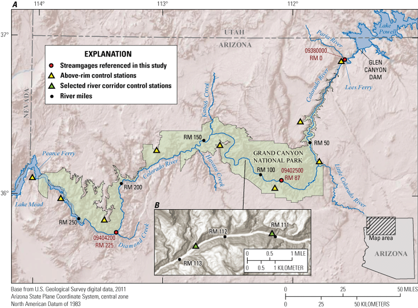
Map of (A) the study reach, the Colorado River in Grand Canyon from Lees Ferry, Arizona, to Pearce Ferry, Ariz., and (B) inset of the river corridor from river miles (RMs) 111 to 113. Streamgages are labeled by RM location, which is distance in miles downstream from Lees Ferry (U.S. Geological Survey, 2025). RM 0 is the Colorado River at Lees Ferry, Ariz. (U.S. Geological Survey station 09380000). RM 87 is the Colorado River near Grand Canyon, Ariz. (U.S. Geological Survey station 09402500). RM 225 is the Colorado River above Diamond Creek near Peach Springs, Ariz. (U.S. Geological Survey station 09404200). Yellow triangles represent the global navigation satellite system (GNSS) base stations in the Grand Canyon Spatial Reference Network (GCSRN) located on the canyon rim that were used for single-base postprocessing (Hazel and others, 2022). Green triangles in the inset map show a subset of river corridor control stations in the GCSRN used for total station surveys. Black dots show selected river miles along the river centerline (Gushue, 2019).
Collecting complete water surface and riverbed profiles can be difficult in Grand Canyon, where the remoteness, extreme topography, and flow regulation complicate surveying efforts. Hydropeaking flows from Glen Canyon Dam result in a fluctuating water surface, steep canyon walls interfere with river-level use of global navigation satellite system (GNSS) receivers, and large rapids and remote terrain make the collection of continuous measurements challenging.
Efforts have been made to measure the profile of the Colorado River for more than 100 years. Complete water surface profiles were collected in 1923 by Birdseye (1928), 40 years prior to closure of Glen Canyon Dam in 1963, and in 2000 by Magirl and others (2005), 37 years after closure of Glen Canyon Dam. Leopold (1969) and Howard and Dolan (1981) measured water depths in many locations between rapids to describe the character of the riverbed, but those measurements were not spatially referenced to a geodetic datum and did not have vertical control and are, therefore, unrepeatable. Although measurements of the riverbed have been taken in segments (Kaplinski and others, 2009, 2017), a complete riverbed profile has not been collected and published.
In 2021, Glen Canyon Dam releases were held nearly constant at a targeted release of 8,000 cubic feet per second (ft3/s) for 7 days during an overflight mission to collect aerial imagery and create a digital surface model (DSM) of the river corridor of the Colorado River in Grand Canyon and its major tributaries (Sankey and others, 2024). During this period, we collected river-based positions using GNSS receivers and total stations and collected bathymetry using multibeam sonar. Using river-based data supplemented with data collected from the overflight, we created the first complete, coupled high-resolution profiles of the water surface and riverbed of the Colorado River from Lees Ferry, Arizona, to Pearce Ferry, Ariz. (fig. 1).
The water surface and riverbed profiles in this report can be used in future studies of channel change, including potential changes in rapids caused by coarse sediment accumulation at debris fans and potential changes in fine sediment storage related to dam operations. The profiles can also be used as inputs for improved models for streamflow and sediment transport that can be used to predict resource responses to future changes in streamflow and dam operations. Such models can improve predictions of changes in sediment resources associated with potential changes in runoff caused by climate change or by revised policies for dam and reservoir management. The results from this study and related studies provide information to stakeholders interested in management of Colorado River water and the natural resources of Grand Canyon National Park, including Federal and State water and resource managers, water and hydroelectric power user groups, recreational and environmental interests, and Native American Tribes.
Study Area, Units, and Datum
The area of study is the corridor of the Colorado River in Grand Canyon National Park from Lees Ferry to Pearce Ferry Rapid (fig. 1). Lees Ferry is 16 miles downstream from Glen Canyon Dam. Pearce Ferry is 298 miles downstream from Glen Canyon Dam and 63 miles downstream from the highest elevation inundated by the Lake Mead reservoir. However, because of low reservoir levels in Lake Mead in the 21st century, Pearce Ferry was about 10 meters (m) above the elevation of Lake Mead reservoir during the study period. Locations along the river corridor are referenced by the convention of river mile (RM), from RM 0.00 at Lees Ferry to RM 281.91 below Pearce Ferry Rapid, with distances increasing downstream (Gushue, 2019).
Horizontal and vertical positions are projected to the Arizona central zone of the State Plane Coordinate System of 1983 in meters (Stem, 1989) and constrained to the 2011 national adjustment of the North American Datum of 1983 (NAD 83 [2011]). Heights and elevations in this report refer to distances in meters above the Geodetic Reference System 1980 ellipsoid defined by NAD 83 (2011). For determining water surface slope, orthometric heights were computed in the North American Vertical Datum of 1988 (NAVD 88) via Geoid18 (Federal Geodetic Control Subcommittee, 1993). Units of streamflow are reported in cubic feet per second.
Discharge During the Study Period
We collected ground- and boat-based data on a river survey mission from May 29 through June 5, 2021, during the period of the overflight imagery and topography mission. During the study period, the hydropeaking flow pattern from Glen Canyon Dam was paused, and dam releases were nearly steady (U.S. Geological Survey, 2025). Discharge at RM 0 (Colorado River at Lees Ferry, Ariz., U.S. Geological Survey station 09380000) was 8,400 ±400 ft3/s (fig. 2A). Discharge increased with distance downstream because of inputs from tributaries. During the steady flow period, flows were 8,800 ±400 ft3/s at RM 87 (Colorado River near Grand Canyon, Ariz., U.S. Geological Survey station 09402500), and 9,100 ±300 ft3/s at RM 225 (Colorado River above Diamond Creek near Peach Springs, Ariz., U.S. Geological Survey station 09404200). At both RM 0 and RM 225, the streamgages where stage was measured during the study period, the range in stage during the steady flow period was less than 0.1 meter (fig. 2B). The tributary with the greatest discharge in the study reach is the spring-fed Little Colorado River, which enters the Colorado River at RM 61. During the study period, the discharge of the Little Colorado River was nearly constant at 218 ±10 ft3/s (Little Colorado River above mouth near Desert View, Ariz., U.S. Geological Survey station 09402300).
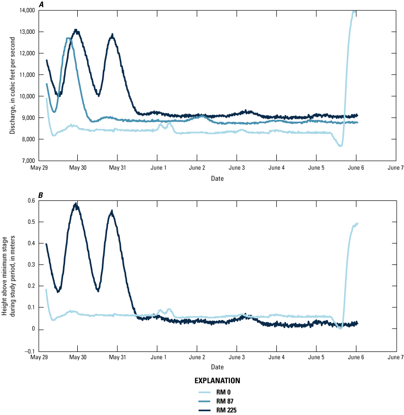
Instantaneous (15-minute) discharge and stage of the Colorado River in Grand Canyon during the study period in 2021 at three streamgages: U.S. Geological Survey stations 09380000 (river mile [RM] 0), 09402500 (RM 87), and 09404200 (RM 225; U.S. Geological Survey, 2025). A, Hydrographs of streamgages at RM 0, 87, and 225 show the transition from hydropeaking to steady flow, beginning at RM 0 on May 29th, 2021, and propagating downstream. Discharge increased in the downstream direction owing to tributary inputs. B, Stage measured at RM 0 and RM 225 is shown as height above the minimum stage during the study period and had a range of less than 0.1 meter during the steady flow period.
Data Collection
This section describes the collection of data used to construct the water surface and riverbed profiles, via boat, aircraft, and shore occupations during the study period (fig. 3). All measurements were referenced to a geodetic control network. Continuous measurements were collected via a moving boat or aircraft using GNSS. Conventional total stations were used to collect standalone water surface height measurements, without relying on GNSS.
Geodetic Control Network
All data were spatially referenced to the National Spatial Reference System (NSRS) through a network of geodetic control points, referred to as the Grand Canyon Spatial Reference Network (GCSRN), which consists of permanent benchmarks established along the canyon rim and the river corridor (Doyle, 1996; Hazel and others, 2022; fig. 1).
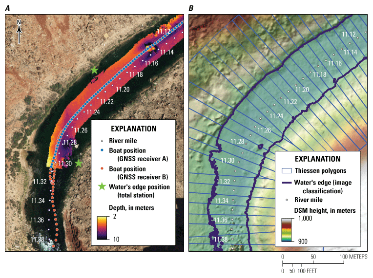
Aerial view of data collected on a section of the Colorado River in Grand Canyon, the river corridor upstream from Soap Creek Rapid (river mile 11.38), showing data collected by river-based survey (A) and aircraft (B). River hundredth miles shown as white dots with every other node labeled. A, Data collected during river survey include boat position and height from two global navigation satellite system (GNSS) receivers [A and B], bathymetry collected by multibeam sonar, and water surface elevations at individual locations collected by using electronic total stations (Sartain and others, 2026). Whereas GNSS receiver A positions and bathymetry were collected only in pools, GNSS receiver B positions were collected in pools and through rapids. The background image is the image collected by the aerial overflight (Sankey and others, 2024). B, Data collected by aircraft include digital images, which were used to classify the water’s edge location (Bransky and others, 2025) and create a digital surface model (DSM) with a 0.20-meter resolution (Sankey and others, 2025), shown here. Thiessen polygons are shown for each river hundredth mile.
Static position data were collected at above-rim geodetic control stations to postprocess river-based data. Static observations from Continuously Operating Reference Stations (CORS) operated by the National Geodetic Survey (NGS) were available from stations in northern Arizona, southern Utah, and southern Nevada (Doyle, 1996). We also deployed eight base stations on above-rim control stations in the GCSRN with positions realized within the NSRS, which were located closer to the edge of the canyon rim than the CORS (Doyle, 1996). Locations of the deployed stations were observed prior to the study by following the procedures described by Zilkoski and others (1997) and were published by following NGS protocols (Doyle, 1996). The average horizontal and vertical accuracies of the eight above-rim control stations referenced in this study are 0.004 m and 0.007 m, respectively (National Oceanic and Atmospheric Administration, 2025a).
Standalone water’s edge locations were measured by using total stations deployed on GCSRN control stations along the river corridor (figs. 1B, 3A). These measurements were used to assess the accuracy of both the continuous GNSS data collected along the river and the overflight imagery (Sankey and others, 2024). Positions of GCSRN control stations along the river corridor and absolute and relative accuracies were acquired prior to the study via a combination of postprocessed GNSS vectors and repetition measurements collected by using total stations through the process of least squares. These control stations have served as primary GNSS constraints for all modern survey-grade data acquisition in this reach (Hazel and others, 2022). The vertical accuracy of the 123 GCSRN stations along the river corridor used in this study averages 0.02 m, and 95 percent of these river stations have a vertical accuracy that does not exceed 0.052 m at 95-percent confidence.
Continuous Measurements of the Water Surface and Riverbed
The primary system used to collect water surface heights and bathymetry was the Norbit iWBMSh multibeam echosounder system. This system consisted of a high-resolution multibeam echosounder (MBES) and an integrated Applanix POS MV OceanMaster inertial navigation system (INS), which included a GNSS receiver with two antennae (collectively referred to as GNSS receiver A hereinafter).
The MBES was mounted on the Research Vessel Frank Protiva, a 5-m inflatable pontoon raft with data collection system electronics housed in a waterproof aluminum box (fig. 4). It was powered by a 50-horsepower 4-stroke outboard motor and able to navigate the rapids of the Colorado River in Grand Canyon. The MBES emits a frequency modulated pulse at 400 kilohertz along a 165-degree swath using 512 0.9- x 1.9-degree beams (NORBIT, 2022). The width of the swath on the riverbed is typically about four times the water depth. A sound velocity probe is attached to the sonar probe to continuously measure the speed of sound near the water surface. Horizontal and vertical position data were acquired by using GNSS receiver A, made up of two 540AP GNSS antennas mounted 1.882 m apart on the canopy at the bow of the vessel. This system also measured vessel heading, roll, pitch, and heave at 50 hertz and logged raw GNSS and inertial observations for use in postprocessing. We used Qinsy version 9.6.2 data collection software (Quality Positioning Services, 2024) on a boat-mounted computer to coordinate, time-tag, and store all the data streams from the MBES system.
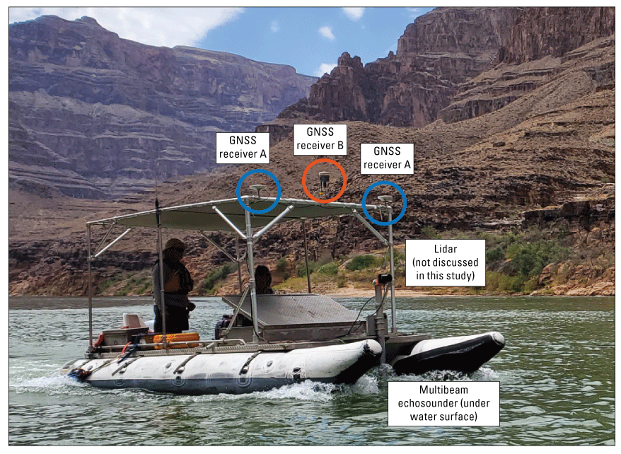
Photograph of the Research Vessel Frank Protiva during the study. Global navigation satellite system (GNSS) antennae for two systems were mounted to a rigid aluminum frame, which also supported a shade canopy. The multibeam echosounder was fixed to the boat with a custom mount, which allowed it to be secured above the water in rapids and deployed in pools, as shown in the photograph. lidar, light detection and ranging. Photograph by Katherine Chapman, U.S. Geological Survey.
Quality assurance procedures were performed immediately prior to data collection to ensure GNSS, MBES, and INS systems were properly calibrated and time-synchronized. Distances between all components’ reference points were measured to the nearest millimeter by using a light detection and ranging (lidar) scanner and total station and verified with careful tape measurements. Patch tests verified system alignments and determined the angular offsets between the sonar head and INS. All offsets were entered into the data collection software. A performance test, also known as a cross-line check, was done to ensure proper system calibration and assess the uncertainty of the bathymetric system, by comparing a “check line” dataset with a “reference surface” dataset constructed from narrowly spaced multibeam data (U.S. Army Corps of Engineers, 2013). Buscombe and others (2014) demonstrated that the water column on the Colorado River is very well mixed, varying only by about 0.2 meter per second from the sound velocity measured at the surface. Therefore, soundings were processed only by using the sound velocity measured at the sonar head.
For data collection, the vessel was driven downstream along the center of current at 5 to 9 knots (9 to 17 kilometers per hour). In most locations, the center of current is near the center of the river channel and is also at or near the river thalweg (deepest part of the channel). Using the real-time display of swath depth below the vessel, we navigated along the deepest path as much as possible. To avoid damaging the sonar head, we only deployed the MBES in deep (greater than 1 m) flatwater and secured it above the water in rapids and through sections of shallow water. The system was turned off before retracting the sonar head, which stopped the collection of positions by GNSS receiver A. Therefore, we employed a secondary system, a single Trimble R10 GNSS receiver (hereinafter referred to as GNSS receiver B), which was also mounted on the canopy at the bow of the vessel (fig. 4). GNSS receiver B collected 1-second kinematic observables throughout the survey, including through rapids and shallow water.
Measurements for Accuracy Assessment
In addition to measuring vessel position with GNSS, we also surveyed the water surface at discrete locations along the water’s edge using conventional total stations (fig. 3A). Because total station measurements have consistent vertical accuracies of 0.02 m or less and were not vulnerable to GNSS outages, they were used to assess the vertical accuracy of all water surface measurements collected in this study.
We measured 578 standalone water’s edge positions from 123 GCSRN river corridor control stations. Each water surface point measured by total station was assigned to the closest river hundredth mile. While some points were singular measurements of water surface height, others were part of water’s edge surveys for accuracy assessments of the aerial imagery and were spaced 1–2 m apart on a line. From RM 0 to RM 226, we measured, on average, one water surface height every approximately 0.4 river mile, though many measurements were clustered along a line. From RM 226 to RM 282, where GCSRN river corridor control stations were sparser, we measured water surface heights at only six locations.
Photogrammetry-Derived Digital Surface Model
For locations where GNSS measurements were of poor quality or not collected, we extracted heights from the water’s edge from the DSM, which was generated via photogrammetry of concurrent aerial images (Sankey and others, 2024, 2025). The DSM is a single-band, continuous raster of 1-m spatial resolution, in which each pixel value represents the elevation of the surface as NAD 83 (2011) ellipsoid height. The DSM represents elevation of open ground (for example, bare soil, rocks, and water) and aboveground features including buildings, trees, and vegetation. As reported by Sankey and others (2025), the vertical difference in meters between GCSRN river corridor control points in the canyon-wide survey control network and associated DSM pixel heights had a root mean square error (RMSE) of 0.70 m (n=926). Vertical accuracy of the DSM at 95-percent confidence was 1.38 m, following the Federal Geographic Data Committee geospatial positioning accuracy standard (Federal Geographic Data Committee, 1998).
Data Processing and Accuracy Analysis
Following data collection, we constructed complete elevation profiles of the water surface and riverbed. This section details the processing steps taken to assess the accuracy of all data and assemble the final water surface profile and bathymetry rasters and profile from the most accurate data available.
Water Surface Profile
Our goal was to construct a continuous profile with vertical accuracy equal to or better than that of previously collected profiles. The first water surface profile collected in this reach was measured in 1923 by stadia rod and level on one continuous river expedition (Birdseye, 1928). The vertical uncertainty of the 1923 profile was 1.4 m, based on calculated closure error at the end of the survey from Lees Ferry (RM 0) to Last Chance Rapid (RM 252; Birdseye, 1928; Magirl and others, 2005). The discharge during the study period varied between 15,000 and 30,000 ft3/s; however, Birdseye (1928) adjusted the elevations measured in 1923 to represent discharge at approximately 10,000 ft3/s, using newly developed stage-discharge ratings.
The next complete water surface profile was constructed by Magirl and others (2005) using water surface measurements made by airborne lidar collected in March 2000. During this study, flows were steady; discharge was approximately 8,200 ft3/s at RM 0 (U.S. Geological Survey, 2025). The absolute vertical accuracy of data used to construct this water surface profile was estimated to be within 0.5 m of true values (Magirl and others, 2005).
In addition to improving upon the vertical accuracy from previous profiles, we also aimed for the uncertainty of our water surface profile to be equal to or better than that of associated discharge measurements. The published uncertainty for “excellent” discharge records published by the U.S. Geological Survey is ±5 percent (Rantz, 1982). In this study, discharge during the steady release period was coincidentally within a range of approximately 5 percent: 8,400 ft3/s (±400 ft3/s; fig. 2A). This amount of variation in discharge resulted in variations in stage of less than 0.1 m where measured during the steady discharge period (fig. 2B). Additionally, based on stage-discharge records for 47 monitoring sites between RM 0 and RM 226, we would expect to see an average change in water surface elevation of ±0.07 m, with a maximum change of ±0.10 m, for changes in discharge of this magnitude (Hazel and others, 2022). Thus, we set ±0.10 m as the target for vertical uncertainty in this study. Comparison to previously collected profiles would need to consider differences in stage as well as vertical error across surveys.
Water Surface Measurements
GNSS observations were processed by using the postprocessed kinematic (PPK) survey method (Rydlund and Densmore, 2012). The PPK method applies differential corrections from simultaneous 1-second observations from above-rim control stations and the vessel’s GNSS rover positions. In this study, static GNSS observations from the nearest canyon rim control station(s) were used to correct the raw observations collected by the GNSS systems on the vessel.
Raw GNSS and INS observations from GNSS receiver A were processed in PosPAC MMS version 8.6 (Trimble, Inc., 2024). Observations were processed by using a single-base method with the nearest above-rim control station. The PPK solution is contained in a smoothed best estimate of vessel trajectory (SBET) file that includes corrected position and motion data and an estimate of uncertainty for each position solution. The SBET was used to update the position and attitude used to locate the raw bathymetric data prior to processing. Following generation of the SBET, we exported positions and precision estimates at 2-second frequency using the bathymetric processing software Qimera version 2.6.2 (Quality Positioning Services, 2023).
Raw GNSS observations from GNSS receiver B were processed in Qinertia version 3.2 (SBG Support Center, 2022). Each file included observations for an average distance of approximately 9 river miles. For each file, the software determined whether a single base station or a virtual base station (VBS) processing method was advantageous; the determination was based on the available base station data relative to the location and trajectory of the vessel during the time window. Where the VBS processing method was used, a VBS was generated from a combination of at least three base stations with static observations made during the time of data collection. This combination included base stations from the 8 above-rim stations we deployed during the study and (or) 11 surrounding CORS. We exported positions and precision estimates at 2-second frequency from the PPK solution.
To generate the water surface profile at the river hundredth-mile resolution, we assigned RM locations at hundredth-mile intervals to the positions of the postprocessed data from the GNSS receivers in Trimble Business Center version 5.4 (Trimble, Inc., 2020) using the published Colorado River centerline (Gushue, 2019). Then, we averaged all positions and precision estimates for each receiver at each river hundredth mile. Per river hundredth mile, there was a median of two 2-second measurements for each receiver. Subsequent discussions of GNSS positions, heights, and precision refer to one averaged value at the river hundredth-mile resolution.
We used two estimates of vertical uncertainty of the GNSS heights to determine which data would be included in the final profile. The first is the quality of the vertical element of the GNSS PPK solution as reported by the respective postprocessing software, which we refer to as the vertical precision (fig. 5). Vertical precision values are positive; low values indicate high precision. The vertical precision values showed that the PPK GNSS solution was reliable for most of the river corridor. Vertical precision values were less than 0.10 m for 91 percent of river miles where measurements were collected by GNSS receiver A and 80 percent of river miles where measurements were collected by GNSS receiver B. Vertical precision was poor (high values) in segments where satellite visibility was limited by canyon orientation and steep canyon walls. The geomorphic reach with the poorest vertical precision was the Muav Gorge (Schmidt and Graf, 1990), in which signals from GNSS satellites to the vessel were obstructed, owing to the dominant east-west orientation and narrow width of the canyon at river level. The average vertical precision in the Muav Gorge reach was 1.2 m for GNSS receiver A and 0.8 m for GNSS receiver B.
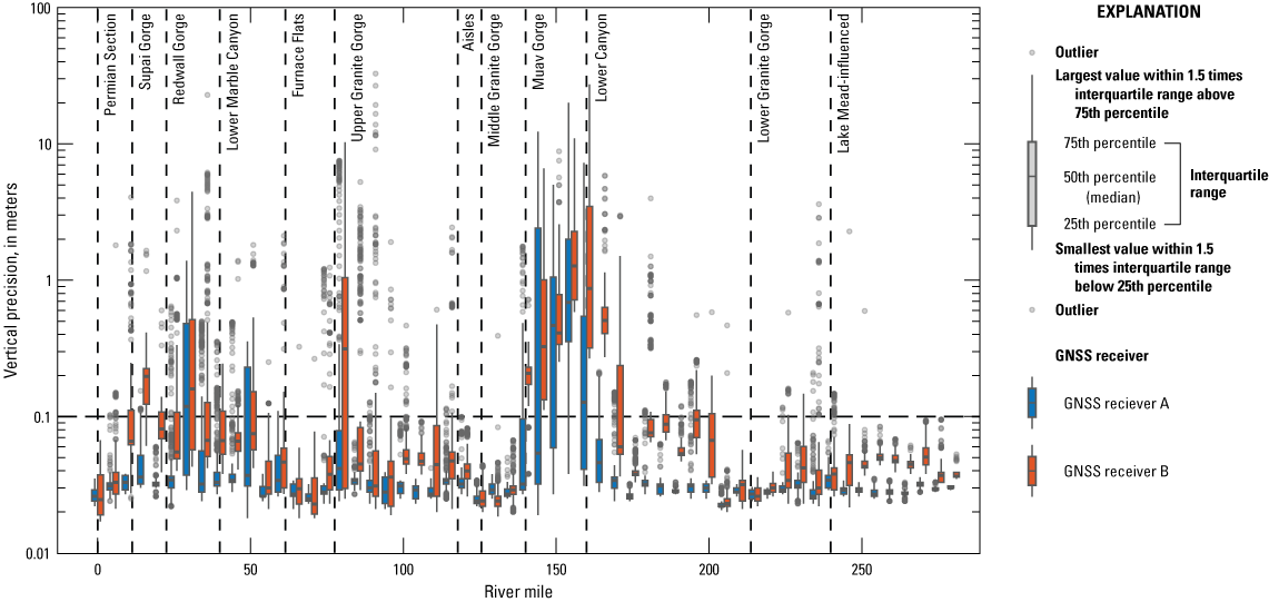
Vertical precision of measurements of the water surface of the Colorado River in Grand Canyon by two global navigation satellite system (GNSS) receivers in 5-mile segments, from Lees Ferry to Pearce Ferry, Arizona (Sartain and others, 2026). Greater values indicate less precise measurements. Vertical dashed lines mark the boundaries of geomorphic reaches, modified from Schmidt and Graf (1990).
The second estimate of vertical uncertainty was the agreement between the heights measured with GNSS and the heights measured independently by total station at the same river hundredth mile, which we refer to as the vertical accuracy (fig. 6). In the cases where we used a total station to measure the water’s edge along a line with points spaced 1–2 m apart, we averaged all heights for each river hundredth mile. This resulted in heights measured by total station at 315 unique river hundredth miles, spaced approximately 0.7 river mile apart on average from RM 0 to RM 225. For each river hundredth mile where we collected both GNSS and total station water surface heights, we calculated the vertical accuracy by subtracting the water surface height measured with total station from the water surface height measured with GNSS:
whereVA
is the vertical accuracy,
HGNSS
is the water surface height measured by GNSS, and
HTS
is the water surface height measured by total station.
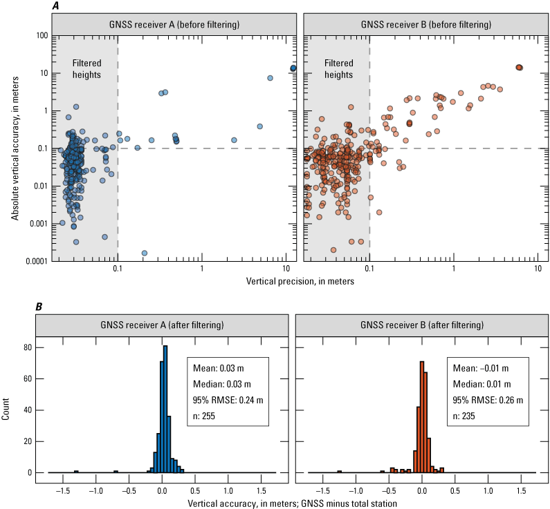
Scatterplots showing absolute vertical accuracy as a function of vertical precision and histograms of vertical accuracy of measurements of the water surface of the Colorado River in Grand Canyon, from Lees Ferry to Pearce Ferry, Arizona, taken by two global navigation satellite system (GNSS) receivers (Sartain and others, 2026). A, GNSS absolute vertical accuracy as a function of vertical precision. Absolute vertical accuracy is the absolute value of the difference between the water surface height surveyed by GNSS and water surface height measured by total station referenced to a geodetic control network at the same river hundredth mile. Greater magnitude values indicate less accurate and less precise measurements. The gray box indicates GNSS heights with an absolute vertical accuracy less than or equal to the threshold of 0.1 meter (m), which are retained after filtering. B, Histogram of vertical accuracies of filtered GNSS heights (only the values from the gray box in panel A). Bins are 0.05 m wide and histogram x-axes are fixed from −1.7 m to 1.7 m. RMSE, root mean square error.
When we evaluated the vertical accuracy of all PPK GNSS solution heights, we found they were mostly accurate; median vertical accuracy was below 0.04 m for both receivers. For several outlier heights, however, the absolute vertical accuracy exceeded 0.1 m and, in a few cases, 10 m. For most of these outliers, poor vertical accuracy was linked to poor vertical precision (fig. 6A). To identify and remove the inaccurate values, we used the associated vertical precision to filter the datasets. For GNSS receiver A measurements with vertical precision less than or equal to 0.10 m, 100 percent were within 0.30 m of the total station measurements and 87 percent were within 0.10 m of the total station measurements. Similarly, for GNSS receiver B system measurements with vertical precision less than or equal to 0.10 m, 99 percent were within 0.30 m of the total station measurements and 93 percent were within 0.10 m.
We used the association between vertical precision and absolute vertical accuracy to filter GNSS measurements, keeping only those with vertical precision values less than or equal to 0.10 m (hereafter referred to as filtered heights; fig. 6B). Vertical accuracies of filtered heights from the two GNSS receivers show agreement with total station heights, with mean absolute vertical accuracies of 0.07 m and 0.07 m and 95-percent RMSE values of 0.24 m and 0.26 m, respectively (table 1). Filtered GNSS receiver heights were available for 246.48 river miles, leaving multiple short segments of the river, totaling 35.55 miles, without heights from either source (fig. 7).
Table 1.
Vertical accuracy statistics relative to total station measurements of three continuous height sources (two global navigation satellite system receivers and a digital surface model) used to create the water surface profile of the Colorado River in Grand Canyon from Lees Ferry to Pearce Ferry, Arizona.[Values calculated from data available in Sartain and others (2026). RMSE, root mean square error; DSM, digital surface model]
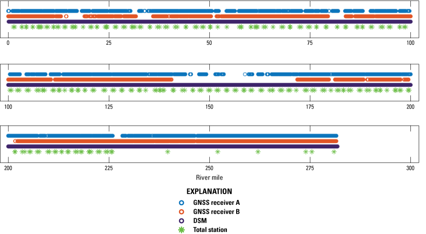
Availability of height measurements of the water surface of the Colorado River in Grand Canyon in 2021, by river mile, used to create a water surface profile, from Lees Ferry to Pearce Ferry, Arizona. Water surface height was measured by two global navigation satellite system (GNSS) receivers, extracted from a concurrent digital surface model (DSM), and measured intermittently by total stations referenced to a geodetic control network (Sartain and others, 2026). The GNSS receiver heights shown here were filtered by their vertical precision value. DSM heights shown here were filtered and smoothed by using total station measurements and a previous water surface profile (Magirl and others, 2005) as a reference.
Photogrammetry-Derived Digital Surface Model
To fill gaps in the water surface profile where heights from the river-based GNSS systems were not collected or had poor accuracy, we created a water surface profile from the DSM derived from concurrently collected aerial images (Sankey and others, 2025; fig. 3B). Although the DSM was calibrated by using GCSRN river corridor control stations from the geodetic control network (Sankey and others, 2025), the calibration was for the height of land topography, not the water. The DSM was not hydro-flattened, and large artifacts were present over the water surface, with some water pixel values exceeding total station measurements by tens of meters. Therefore, rather than use the height of water pixels, we estimated water surface height from the DSM using height values of the land surface along the water’s edge.
We extracted heights from the DSM along the water’s edge using a map of surface water that was classified by Bransky and others (2025) from the aerial imagery collected during the study period (Sankey and others, 2024). Bransky and others (2025) evaluated the accuracy of the water’s edge line by comparing its horizontal position to the 385 positions that were measured by total station along a water’s edge line at 24 sandbars during this study. The average horizontal distance between the classified water’s edge and surveyed water’s edge was 0.27 m, and 95 percent of the distances were less than 0.83 m.
We assigned heights to the water’s edge boundary, derived from the DSM, at 1-m intervals (the pixel size). We then assigned a river hundredth mile to each 1-m location along the water’s edge. To do so, we created Thiessen polygons from the river centerline (Gushue, 2019) so that each polygon captured all locations closer to the corresponding hundredth-mile node than any other node and was wide enough to include the left and right riverbanks (fig. 3B). A mean of 77 water’s edge pixels at 1-m resolution were sampled within each river hundredth-mile polygon, though this number varied greatly. Some river hundredth-mile polygons contained more than 800 water’s edge pixels because of complex shorelines, islands, or many rocks partially submerged by water, all of which increased shoreline length.
For river hundredth miles where water surface height was measured by total station, we calculated the vertical accuracy of the corresponding sampled DSM water’s edge heights (fig. 8). Many DSM water’s edge heights were positively biased relative to true heights (fig. 8A), such as in places with sheer cliffs at river level.
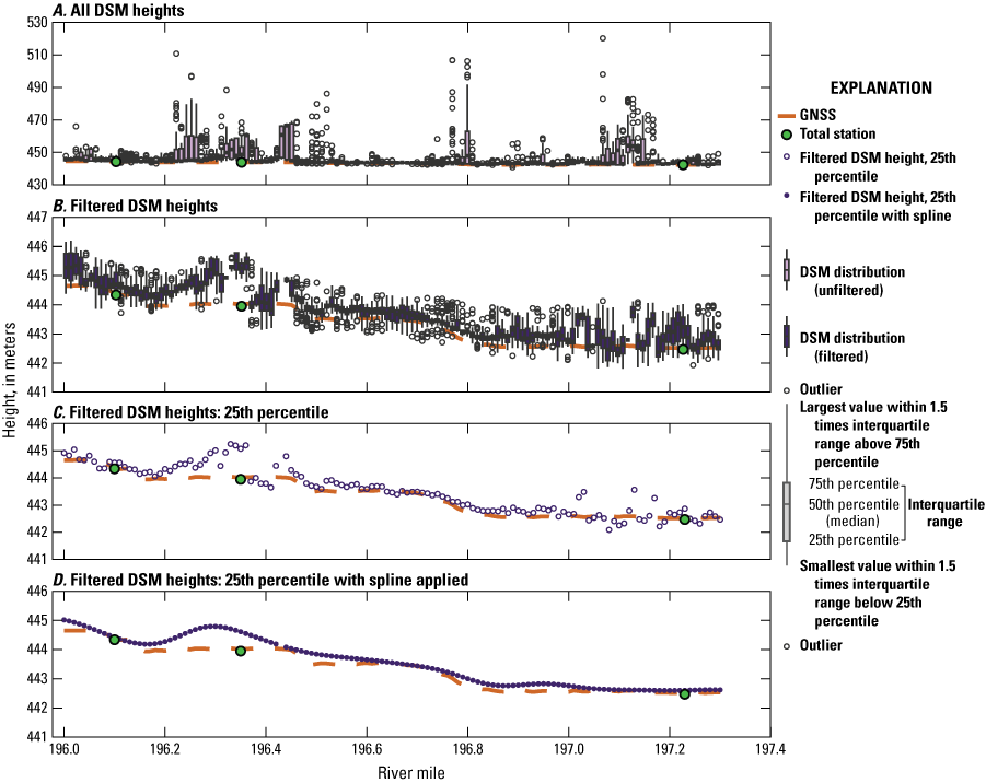
Process for generating a water surface profile for the Colorado River through Grand Canyon, from Lees Ferry to Pearce Ferry, Arizona, from a digital surface model (DSM) collected via overflight photogrammetry in 2021 during the study period (Sankey and others, 2025; Sartain and others, 2026). The DSM-generated profile, a section of which is shown here, was used to fill in water surface heights where global navigation satellite system (GNSS) survey data were not available. A, All DSM heights, collected every 1 meter along a delineated water’s edge line (Bransky and others, 2025), by river hundredth mile for a section of the study area, river miles 196.00 to 197.30. B, DSM heights remaining after removing heights that differed from the 2000 water surface profile (Magirl and others, 2005) by more than 2 meters and applying a moving window filter. C, 25th percentile of the distribution of filtered water’s edge heights at each river hundredth mile. D, The final DSM-derived water surface profile after applying a spline with 3,000 knots to the 25th percentile of filtered data (panel C).
To better estimate water surface heights from the DSM at the hundredth-mile resolution, we took multiple steps to remove outliers. First, we used the profile collected most recently in 2000 by Magirl and others (2005) to estimate expected deviations in water surface height. We converted water surface elevations measured in 2000 relative to the National Geodetic Vertical Datum of 1929 to ellipsoid heights relative to NAD 83 (2011), using the National Geodetic Survey Coordinate Conversion and Transformation Tool (National Oceanic and Atmospheric Administration, 2025b). Because the 2000 water surface profile was reported only at inflection points, we used linear interpolation to generate a water surface height value for every river hundredth mile.
We found that 99 percent of filtered GNSS heights measured in this study were within 1.21 m of the 2000 profile at the same river mile. In addition, a debris flow occurred in August of 2016 at Granite Springs (RM 220.6), which enlarged the debris fan. Preliminary, unpublished data, collected by the U.S. Geological Survey in 2016, show an increase in water surface height by about 1.5 m. We did not expect to see changes in water surface height greater than 1.5 m, especially those exceeding 2 m, in the reaches where the DSM water surface profile would be used, such as the Muav Gorge. Therefore, we removed DSM heights with a difference of 2 m or more from the 2000 profile. We used a 2-m threshold to ensure that we were removing outliers caused by DSM artifacts rather than real changes in the longitudinal profile in the intervening period. Because the 2000 profile was only reported from RMs 0 to 230.13, we could not remove outlier DSM heights from RMs 230.14 to 281.91 at this step. However, downstream from RM 230.13, filtered GNSS heights were available for 97 percent of the river, so the DSM profile was used for only 3 percent of this reach. Filtering by the 2000 profile removed 13.4 percent of all 1-m sampled DSM water’s edge heights.
Following the removal of outlier DSM heights using the 2000 profile for the segments of river specified above, additional outliers remained. We next applied a moving window filter to the remaining DSM heights. For each river hundredth-mile node, we calculated the mean and standard deviation of all remaining 1-m samples collected from the surrounding 0.2 river mile and removed height values more than two standard deviations greater or less than the mean. This removed an additional 3.1 percent of sampled DSM water’s edge heights. Because of the moving window filter, no DSM water’s edge remained for RMs 0 to 0.09 and 281.82 to 281.91. After the removal of outliers using the 2000 water surface profile and the moving window filter, an average of sixty-four 1-m-height samples remained per river hundredth mile; hereafter, these samples are referred to as filtered DSM heights (fig. 8B). At 141 river hundredth-mile nodes (1.41 total river miles), the filtering process removed all DSM heights (for example, at RM 196.43 in fig. 8).
To assign a single height to each river hundredth mile, we compared multiple summary statistics of the distribution of filtered DSM heights (for example, minimum, 10th and 25th percentile, and median) to use in calculating the vertical accuracy. The minimum and 10th percentile of the filtered DSM heights each underestimated total station heights by more than 0.15 m on average, and the median overestimated by more than 0.25 m on average. The 25th percentile of the filtered DSM heights best represented the total station heights, with a median vertical accuracy of −0.02 m (fig. 8C).
Finally, to reduce noise present in the 25th percentile of filtered heights without smoothing over the pool-rapid morphology, we applied a spline with 3,000 knots (Chambers and Hastie, 1992) to the 25th percentile of the filtered DSM heights (fig. 8D). The final DSM heights, after filtering and applying a spline, had a median vertical accuracy of 0.02 m, mean absolute vertical accuracy of 0.19 m, and 95-percent RMSE of 0.52 m (fig. 9; table 1).
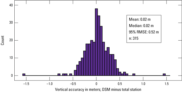
Histogram of vertical accuracy of water surface heights of the Colorado River in Grand Canyon, from Lees Ferry to Pearce Ferry, Arizona, collected from the digital surface model (DSM), filtered, and smoothed (Sartain and others, 2026). Vertical accuracy is the difference between the DSM-derived water surface height and water surface height measured by total station at the same river hundredth mile; greater magnitude values indicate lower accuracy. Bins are 0.05 meter (m) wide and histogram x-axis is fixed from −1.6 m to 1.6 m. RMSE, root mean square error.
Assembling the Final Water Surface Profile
Following filtering of each data source, in many cases multiple height sources per river hundredth mile were available to create the water surface profile (figs. 7, 10A; table 1). To assemble the profile with one value per river hundredth mile, we used a tiered system. First, we assigned filtered GNSS receiver A heights to all river miles where available because of the integration of the GNSS receiver with the MBES system (201.57 total river miles). Then, where filtered GNSS receiver A heights were not available, we used filtered GNSS receiver B heights (44.89 total river miles). Where heights were not available from either GNSS receiver, we used the filtered, smoothed DSM-derived water’s edge heights with the spline applied (35.36 total river miles). We refer to this profile, created from the combination of filtered GNSS receiver and DSM heights, as the measured profile (fig. 10B).
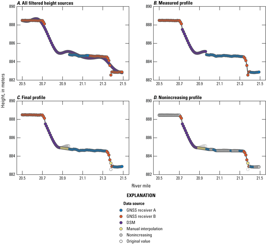
Process for creating the final and nonincreasing water surface profiles of the Colorado River in Grand Canyon, from Lees Ferry to Pearce Ferry, Arizona, using water surface height from multiple sources (Sartain and others, 2026). A, All filtered heights for river miles 20.5 to 21.5, collected by two global navigation satellite system (GNSS) receivers and a concurrent digital surface model (DSM). B, Measured profile created by selecting one height source per river hundredth mile, with priority for GNSS receiver A, then GNSS receiver B, then the DSM. C, Final profile following manual interpolation to smooth the transition between data sources and vessel pitch (drops and rebounds in rapids). Where adjusted, original data are shown as empty gray circles. D, Nonincreasing profile created for resource modeling, where elevation does not increase with distance downstream. Adjustments are shown as gray points.
The filtering steps described above removed nearly all potentially inaccurate heights from the water surface profile. However, some heights were within the level of error for the given source but were visibly incorrect at the point of transition to a height source of greater accuracy (for example, at RM 20.95 in fig. 10B). Other incorrect heights were evident at locations where the research vessel dropped and rebounded in a rapid (for example, at RM 21.39 in fig. 10B). Where such inaccuracies could be confidently identified, especially in cases where the drop below a rapid was well below the elevation of the downstream pool, we deleted individual heights or short segments and replaced those values using linear interpolation between the nearest remaining heights (fig. 10C). This manual interpolation was performed for 11.29 individual river hundredth mile nodes (11.29 river miles total, 4 percent of the profile). The average length of the interpolated segments was 0.06 river mile, and the mean absolute change of the heights of the interpolated nodes was 0.19 m. Following the final step of manual interpolation, we report this as the final water surface profile (fig. 10C).
Creating a Nonincreasing Water Surface Profile
In places where we could not visually identify standalone, inaccurate heights, some instances of water surface height increasing downstream remained. Examples include subtle fluctuations in flat pools on the order of decimeters or less (for example, at RMs 21.0 to 21.3 in fig. 10B) or some places where heights from the DSM were used (for example, at RM 196.3 in fig. 8D). Because the water surface profile is intended to be used for modeling of river resources, we aimed to create a version in which height did not increase with distance downstream; this can cause problems in hydraulic models (fig. 10D). We created the nonincreasing water surface profile from the final water surface profile. If water surface heights increased downstream, they were held constant until the next decreasing value. This resulted in constant heights for a total of 136.88 river miles, just under half of the profile. Almost all of these adjustments were in flat pools. The average adjustment to heights in the nonincreasing profile was 0.04 m (all changes resulted in lower heights), with a standard deviation of 0.05 m.
Riverbed Profile
Bathymetric data were processed and edited by using Qimera version 2.6.2 (Quality Positioning Services, 2023). First, we verified that all system offsets were properly applied. These offsets include horizontal and vertical distances between system components and angular offsets measured through the patch test. Next, we assigned vertical and horizonal positions to the soundings from the PPK Applanix SBET file.
The results of the performance test, conducted prior to data collection using real-time kinematic GNSS positioning, showed that the system was well calibrated. The difference between the check line and reference surface datasets across all beamwidths (−70 to 70 degrees) had a mean of 0.04 m and a 95-percent RMSE of 0.11 m. The result of the performance test served as an indicator of vertical uncertainty for the bathymetric surfaces.
MBES data collected in shallow, fast-moving rivers are inherently noisy because of a combination of steep slopes, topographic complexity, side-lobe effects, multipath effects, water-column targets (for example, air bubbles and suspended particles), and ambient high-frequency noise (Kaplinski and others, 2009). Based on the authors’ experience, automated filters can be unreliable in this environment. Visually inspecting and manually editing MBES data collected on the Colorado River in Grand Canyon is considered more reliable (Kaplinski and others, 2009; 2017, p. 201; 2022; Wright and others, 2024). Editing MBES soundings manually involved visually inspecting the soundings at intervals of approximately 5 m and rejecting soundings that did not represent the riverbed. After this process was completed, we generated a 1-m-resolution digital elevation model (DEM).
Following editing, the resulting DEM contained multiple instances of visible, abrupt horizontal and vertical displacement of riverbed bathymetry, in the isolated sections with the least accurate PPK solutions for GNSS receiver A. Visual inspection of the riverbed elevation profile showed that bathymetry in some areas, mainly those within narrow geomorphic reaches where GNSS receiver A observations on the vessel were sparse, remained unacceptable because of abrupt horizontal offsets or inaccurate heading. In these places, where soundings were obviously in the wrong place, such as appearing to be within the canyon walls or abruptly scattered, we removed all soundings from the final surface.
Where horizontal positioning and heading were correct, accurate vertical positioning remained difficult to achieve in some reaches, usually those with poor PPK solutions as reported by the vertical uncertainty estimate (figs. 5, 6). Rather than use GNSS receiver A data alone to position the bathymetric soundings, we took a novel approach and generated a tide file from the final water surface profile constructed from the two GNSS receivers and DSM with minimal manual interpolation (fig. 10C). Tide files, representing the tide levels of a body of water over time, can be used for vertical positioning of multibeam sonar surveys, though typically in ocean or estuary settings. We created a file with the final water surface heights at a 2-second resolution, linking a final water surface height to each timestamp of the full-resolution data from the two GNSS receivers via the river hundredth mile. We then used the tide file to recalculate the height of the riverbed from the depth measured by the echosounder, accounting for differences in water surface and the acoustic center of the sonar head, or “draft.” We did not substitute horizontal positions. Of the more than 230 river miles where bathymetry was measured (in other words, not in rapids), approximately 89 percent of water surface heights used in the final water surface profile were from GNSS receiver A and therefore largely unchanged, approximately 7 percent were changed to photogrammetry-derived DSM heights, less than 1 percent were changed to GNSS receiver B heights, and 4 percent were changed to interpolated heights.
We also created a raster of riverbed depths by removing the vertical elevation source and adjusting the soundings by the draft. This raster was unaffected by the tide file substitution. Both versions of the final riverbed elevation profiles (elevation and depths) were processed by using Qimera version 2.6.2 and exported as floating point GeoTIFF raster files with 1-m resolution.
Values for riverbed height and depth were assigned to each river hundredth mile by extracting statistics from the bathymetric rasters. For each river hundredth-mile Thiessen polygon (fig. 3B), we identified the deepest location by extracting the 99th percentile of measured depths; correspondingly, for the elevation raster, we extracted the 1st percentile of measured heights. We used the 99th and 1st percentiles rather than the maximum and minimum, respectively, to exclude outliers. Because the vessel was at or near the deepest part of the channel and because the MBES measured depths in a swath, these minimum riverbed elevations represent the thalweg—not necessarily the centerline depth.
The sum of the riverbed heights and depths, reported by river hundredth mile, nearly equaled but was not identical to the final water surface profile (95-percent RMSE = 0.04 m, mean absolute error = 0.01 m). The difference between these two values was greater in places with fewer bathymetric pixels per hundredth mile and at the start and end of bathymetric survey segments. At the beginning and end of survey segments, this difference was primarily due to discrepancies resulting from a slight difference in how river miles were assigned to the GNSS (vector) data versus the bathymetric (raster) data, which were then expressed in the tide file. The final water surface profile is reported in hundredth mile increments and, to create the tide file, was scaled up to 2-second-resolution data by using the corresponding river mile. Because of the slight misalignment of river miles, in some cases in the tide file, a bathymetric segment was positioned entirely with GNSS receiver A heights, and a different data source was used for only the very start and (or) end. To account for this, we did not include thalweg depth or elevation in the final profile from the first or last 0.02 river mile of each bathymetric segment (2.4 percent of river miles with bathymetric data). We also did not include thalweg depth or elevation in the final profile for river miles with fewer than 100 1-m pixels (1.1 percent of river miles with bathymetric data). Despite these discrepancies, which resulted in errors on the order of centimeters, the use of the tide file greatly improved the heights of nearly 20 river miles of bathymetric data that were previously positioned with less accurate GNSS receiver A solutions; improvements were by tens of meters in some cases. Following removal of these thalweg values from the final profile, the 95-percent RMSE between the bathymetric depth plus the bathymetric height relative to the water surface height was 0.03 m (mean absolute error = 0.01 m). This is well within the 0.10 m target vertical error of the overall survey.
Analysis by Geomorphic Reach
We summarized water surface and riverbed elevation characteristics by geomorphic reach (table 2). The reaches defined by Schmidt and Graf (1990) end at Diamond Creek (RM 225); however, data in this study were collected to downstream from Pearce Ferry and end at RM 281.81. We modified the Schmidt and Graf (1990) reaches to include the section of river from Diamond Creek to Pearce Ferry. We extended the Lower Granite Gorge geomorphic reach downstream to Separation Canyon (RM 239.79). We added a “Lake Mead-influenced” reach that extends from Separation Canyon (RM 239.80) to downstream from Pearce Ferry Rapid (RM 281.81). Although the level of Lake Mead during the time of the study was downstream from the surveyed reach, Lake Mead reservoir can extend upstream to RM 235.3 at full pool. However, reservoir levels have been below the elevation at Separation Canyon more than 80 percent of the time since 1935 and have not been above that location since 2001. Downstream from Separation Canyon are Colorado River sediment deposits in the former reservoir delta from the more than 90 years of Lake Mead, including sediments from the nearly 40 years during the period before Glen Canyon Dam cut off upstream sediment supply. This reservoir sediment has buried the predam riverbed, in some places by tens of meters, as well as the debris fans that constrict the channel.
Table 2.
Characteristics by geomorphic reach of the Colorado River in Grand Canyon from Lees Ferry to Pearce Ferry, Arizona.Reaches modified from Schmidt and Graf (1990).
River miles were updated from Schmidt and Graf (1990) to reflect the most recently published Colorado River centerline (Gushue, 2019).
Slope was calculated by using the elevation of the final water surface profile in the North American Vertical Datum of 1988.
Thalweg depth was calculated for each river hundredth mile as the 99th percentile of bathymetric depth. Maximum thalweg depth was the greatest thalweg depth in each geomorphic reach.
Channel width was calculated by dividing the area of water polygon from Bransky and others (2025) by geomorphic reach length in meters.
To calculate the slope of the water surface for each geomorphic reach, we converted water surface ellipsoid heights in NAD 83 (2011) to elevations relative to NAVD 88. NAVD 88 elevations are referenced to the geoid, which accounts for spatial variability in Earth’s gravity, and are therefore more appropriate for calculating slope of the water surface than are ellipsoid heights. We calculated slope for each geomorphic reach using the length of the reach along the centerline vector, in meters.
We also calculated riverbed statistics for each geomorphic reach. For each reach, we calculated the maximum thalweg depth (in other words, the deepest pool) and the mean thalweg depth of the places where bathymetry was collected, in pools. Lastly, we used the water’s edge polygon (Bransky and others, 2025) to measure channel width for each geomorphic reach by dividing the water boundary polygon area, in square meters, by reach length, in meters.
Results
The final continuous water surface profile with a height every hundredth mile (16.1 m) was based primarily on postprocessed heights from GNSS receiver A but includes heights from all three measurement systems and some interpolation (fig. 10C; Sartain and others, 2026). Heights were derived from GNSS receiver A for 73 percent (206.59 river miles) of the 282-mile profile, with mean absolute vertical accuracy of 0.07 m (95-percent RMSE = 0.24 m). Heights were derived from GNSS receiver B for 12 percent (34.05 river miles) of the profile, also with mean absolute vertical accuracy of 0.07 m (95-percent RMSE = 0.26 m). Heights were from the DSM for 11 percent (29.65 river miles) of the profile for which river-based GNSS observations were unreliable. DSM heights had a mean absolute vertical accuracy of 0.19 m (95-percent RMSE = 0.52 m). For the remaining 4 percent (11.53 river miles) of the profile, heights were interpolated between measured water surface heights, either because they were selected (11.29 river miles) or because no data were available (0.24 river mile). A nonincreasing water surface profile was also constructed to be used for modeling of river resources (fig. 10D).
The bathymetric data were used to create a raster for riverbed heights along the vessel track that is in the same datum as the water surface heights. A second raster, representing depth below the water surface, was also produced. A thalweg profile was created by computing the minimum riverbed height (99th percentile depth) at each river hundredth mile. Water surface height, channel thalweg height, and channel thalweg depth are all tabulated by river hundredth mile according to Thiessen polygons generated along the centerline vector of Gushue (2019).
The final water surface and riverbed profiles show the drop for each individual rapid and the large variations in depth that occur between the shallow sections near each rapid and the deep pools (fig. 11, app. 1). The Lake Mead-influenced reach had the lowest gradient, shallowest maximum and mean thalweg depths, and greatest width, because of the accumulation of Lake Mead reservoir sediments that have buried the predam channel (table 2, app. 1). Excluding the Lake Mead-influenced reach, average slope ranged from 0.00092 (4.9 feet per mile) in the Permian Section to 0.00208 (11.0 feet per mile) in the Upper Granite Gorge (table 2). Maximum pool depth excluding the Lake Mead-influenced reach ranged from 18.64 m in the Muav Gorge to the deepest location of 28.43 m in the Middle Granite Gorge (table 2; fig. 11).
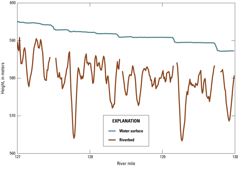
Profile of surveyed water surface and riverbed elevations for river miles 127 to 130 of the Colorado River in Grand Canyon (Sartain and others, 2026). Riverbed elevation approximates the thalweg depth. Gaps in the riverbed profile often correspond to rapids (drops in the water surface profile), where riverbed elevations were not measured. This section shows the deepest pool on the Colorado River in Grand Canyon National Park, which is at river mile 127.78 and is 28.43 meters deep. Profiles for the entire study reach are included as appendix 1.
Conclusions
Following a unique opportunity of concurrent collection of airborne imagery, global navigation satellite system (GNSS) observations of water surface height, and measurements of river channel bathymetry during a steady flow in 2021, we constructed the first complete and coupled continuous profiles of water surface and riverbed heights along the approximate centerline of the Colorado River in Grand Canyon.
Although many modern studies of landforms and river systems rely exclusively on GNSS observations, in remote environments with obstructed views of the sky, this reliance can result in large errors and gaps in data. In this study, rather than rely entirely on river-based GNSS observations, we incorporated a concurrently collected digital surface model and independent terrestrial ground-truth observations tied to a common geodetic control network. Using the terrestrial ground-truth observations as a reference, we removed GNSS heights that did not meet precision criteria and substituted in digital surface model heights that were filtered and smoothed.
Combining multiple height sources using a tiered system based on vertical accuracy allowed us to create a continuous water surface profile with height to within 0.07-meter mean absolute vertical accuracy for 85 percent of the river corridor, where height was measured by GNSS. For 11 percent of the river corridor, we substituted the vessel-based measurements with data from the digital surface model, which were constrained to ground-truth measurements, resulting in 0.19-meter mean absolute vertical accuracy. We interpolated between measured heights for the remaining 4 percent of the river corridor.
The only previously collected water surface profile that included this entire reach was collected in 1923, 40 years prior to the completion of Glen Canyon Dam. A profile collected in 2000 included only the reach from Lees Ferry to Diamond Creek. Both earlier surveys had unconstrained uncertainty owing to collection methods, lack of independent data verification, and, in the case of the 1923 survey, unregulated discharge. Although some previous studies measured continuous profiles of the river depth, comparing those profiles to newly collected data may not be possible because they were not referenced to any vertical datum.
This study establishes an approach and workflow to create similar water surface and riverbed profiles during any potential future overflight operation in which Glen Canyon Dam releases are held constant. The water surface and riverbed profiles created here were used to summarize geomorphic characteristics by reach, providing updated conditions particularly for the reach impacted by Lake Mead. They can be compared to water surface profiles collected by Birdseye (1928) and Magirl and others (2005) and previous bed elevation measurements. This study’s profiles can inform ongoing studies of the effects of Glen Canyon Dam on the Colorado River in Grand Canyon by providing updates on geomorphic conditions, which are critical for resource modeling.
References Cited
Birdseye, C.H., 1928, Topographic instructions of the United States Geological Survey. Introduction: U.S. Geological Survey Bulletin 788, 432 p., accessed December 1, 2023, at https://doi.org/10.3133/b788.
Bransky, N.D., Sartain, S.L., and Sankey, J.B., 2025, Water classification of the Colorado River Corridor, Grand Canyon, Arizona, 2021—Data: U.S. Geological Survey data release, accessed April 16, 2025, at https://doi.org/10.5066/P13SRUPW.
Bureau of Reclamation, 2026, Lower Colorado River operations—Lake Mead at Hoover Dam, end of month elevation (feet): Bureau of Reclamation data, accessed April 27, 2026, at https://www.usbr.gov/lc/region/g4000/hourly/mead-elv.html.
Buscombe, D., Grams, P.E., and Kaplinski, M.A., 2014, Characterizing riverbed sediment using high-frequency acoustics—1. Spectral properties of scattering: Journal of Geophysical Research: Earth Surface, v. 119, no. 12, p. 2674–2691, accessed January 16, 2024, at https://doi.org/10.1002/2014JF003189.
Doyle, D.R., 1996, Development of the National Spatial Reference System: Silver Spring, Md., National Oceanic and Atmospheric Administration, accessed April 16, 2025, at https://www.ngs.noaa.gov/PUBS_LIB/develop_NSRS.html.
Federal Geodetic Control Subcommittee, 1993, Affirmation of vertical datum for surveying and mapping activities: Federal Register, v. 58, no. 120, accessed May 30, 2025, at https://www.ngs.noaa.gov/PUBS_LIB/FedRegister/FRdoc93-14922.pdf.
Federal Geographic Data Committee, 1998, Geospatial positioning accuracy standards, Part 3—National Standard for Spatial Data Accuracy: Federal Geographic Data Committee FGDC–STD–007.3–1998, 25 p., accessed May 30, 2025, at https://www.fgdc.gov/standards/projects/accuracy/part3/chapter3.
Graf, W.L., 1980, The effect of dam closure on downstream rapids: Water Resources Research, v. 16, no. 1, p. 129–136, accessed January 8, 2024, at https://doi.org/10.1029/WR016i001p00129.
Grams, P.E., Buscombe, D., Topping, D.J., Kaplinski, M., and Hazel, J.E., Jr., 2019, How many measurements are required to construct an accurate sand budget in a large river? Insights from analyses of signal and noise: Earth Surface Processes and Landforms, v. 44, no. 1, p. 160–178, accessed August 21, 2018, at https://doi.org/10.1002/esp.4489.
Gushue, T., 2019, Colorado River Mile System, Grand Canyon, Arizona: U.S. Geological Survey data release, accessed November 10, 2022, at https://doi.org/10.5066/P9IRL3GV.
Hanks, T.C., and Webb, R.H., 2006, Effects of tributary debris on the longitudinal profile of the Colorado River in Grand Canyon: Journal of Geophysical Research: Earth Surface, v. 111, no. F2, p. 1–13, accessed September 21, 2022, at https://doi.org/10.1029/2004JF000257.
Hazel, J.E., Jr., Kaplinski, M.A., Hamill, D., Buscombe, D., Mueller, E.R., Ross, R.P., Kohl, K., and Grams, P.E., 2022, Multi-decadal sandbar response to flow management downstream from a large dam—The Glen Canyon Dam on the Colorado River in Marble and Grand Canyons, Arizona: U.S. Geological Survey Professional Paper 1873, 104 p., accessed December 5, 2022, at https://doi.org/10.3133/pp1873.
Howard, A., and Dolan, R., 1981, Geomorphology of the Colorado River in the Grand Canyon: The Journal of Geology, v. 89, no. 3, p. 269–298, accessed December 5, 2022, at https://doi.org/10.1086/628592.
Kaplinski, M., Hazel, J.E., Jr., Grams, P.E., Gushue, T., Buscombe, D.D., and Kohl, K., 2022, Channel Mapping of the Colorado River from Glen Canyon Dam to Lees Ferry in Glen Canyon National Recreation Area, Arizona: U.S. Geological Survey Open-File Report 2022–1057, 20 p., accessed November 2, 2023, at https://doi.org/10.3133/ofr20221057.
Kaplinski, M., Hazel, J.E., Jr., Grams, P.E., Kohl, K., Buscombe, D.D., and Tusso, R.B., 2017, Channel mapping of the Colorado River in Grand Canyon National Park, Arizona—May 2009, river miles 29 to 62—Data: U.S. Geological Survey data release, accessed April 16, 2025, at https://doi.org/10.5066/F7930RCG.
Kaplinski, M., Hazel, J.E., Jr., Parnell, R., Breedlove, M., Kohl, K., and Gonzales, M., 2009, Monitoring fine-sediment volume in the Colorado River ecosystem, Arizona—Bathymetric survey techniques: U.S. Geological Survey Open-File Report 2009–1207, 33 p., accessed January 16, 2024, at https://doi.org/10.3133/ofr20091207.
Kieffer, S.W., 1985, The 1983 hydraulic jump in Crystal Rapid—Implications for river-running and geomorphic evolution in the Grand Canyon: The Journal of Geology, v. 93, no. 4, p. 385–406, accessed January 8, 2024, at https://doi.org/10.1086/628962.
Leopold, L.B., 1969, The rapids and the pools—Grand Canyon, chap. D of The Colorado River Region and John Wesley Powell: U.S. Geological Survey Professional Paper 669, 145 p., accessed October 3, 2022, at https://doi.org/10.3133/pp669D.
Magirl, C.S., Webb, R.H., and Griffiths, P.G., 2005, Changes in the water surface profile of the Colorado River in Grand Canyon, Arizona, between 1923 and 2000: Water Resources Research, v. 41, no. 5, p. 1–19, accessed October 3, 2022, at https://doi.org/10.1029/2003WR002519.
National Oceanic and Atmospheric Administration, 2025a, Finding survey marks and datasheets: National Geodetic Survey web page, accessed May 30, 2025, at https://geodesy.noaa.gov/datasheets/.
National Oceanic and Atmospheric Administration, 2025b, NGS Coordinate Conversion and Transformation Tool (NCAT): National Geodetic Survey web page, accessed June 27, 2025, at https://www.ngs.noaa.gov/NCAT/.
NORBIT, 2022, NORBIT—iWBMS multibeam sonar system: NORBIT datasheet -PS-120006-24, 2 p., accessed April 27, 2026, at https://norbit.com/api/file/PS-120006-24_iWBMS_A4.pdf.
Quality Positioning Services, 2023, Qimera 2.6.2 release [release notes]: Quality Positioning Services web page, accessed April 27, 2026, at https://qpssoftware.scrollhelp.site/qimera/qimera-2-6-2-release.
Quality Positioning Services, 2024, Qinsy 9.6.2 release [release notes]: Quality Positioning Services web page, accessed April 27, 2026, at https://qpssoftware.scrollhelp.site/qinsy/qinsy-9-6-2-release.
Rantz, S.E., 1982, Measurement and computation of streamflow—Volume 1. Measurement of stage and discharge: U.S. Geological Survey Water-Supply Paper 2175, p. 1–284, accessed May 12, 2025, at https://doi.org/10.3133/wsp2175.
Rydlund, P.H., Jr., and Densmore, B.K., 2012, Methods of practice and guidelines for using survey-grade global navigation satellite systems (GNSS) to establish vertical datum in the United States Geological Survey: U.S. Geological Survey Techniques and Methods, book 11, chap. D1, 102 p., accessed May 15, 2025, at https://doi.org/10.3133/tm11D1.
Sankey, J.B., Bransky, N.D., Kohl, K.A., Gushue, T.M., Bedford, A.F., and Durning, L.E., 2025, Digital elevation model (DEM) and digital surface model (DSM) data for the Colorado River corridor in Grand Canyon National Park and Glen Canyon National Recreation Area (2002, 2009, 2013 and 2021), including accuracy assessment data: U.S. Geological Survey data release, https://doi.org/10.5066/P93Y4FMJ.
Sankey, J.B., Bransky, N., Pigue, L., Kohl, K., and Gushue, T.M., 2024, Four band image mosaic of the Colorado River Corridor in Arizona—2021, including accuracy assessment data: U.S. Geological Survey data release, accessed January 27, 2025, at https://doi.org/10.5066/P9BBGN6G.
Sartain, S.L., Kaplinski, M.A., Kohl, K., Chapman, K.A., Bransky, N.D., Sankey, J.B., and Grams, P.E., 2026, Continuous and high-resolution profiles of the water surface and riverbed elevation for 282 miles of the Colorado River from Lees Ferry to Pearce Ferry, AZ, 2021—Data: U.S. Geological Survey data release, https://doi.org/10.5066/P135FNFM.
SBG Support Center, 2022, Qinertia 3.2.881-stable: SBG Support Center software release, accessed April 27, 2026, at https://support.sbg-systems.com/sc/qd/latest/download-release-notes/qinertia-3-2-881-stable.
Schmidt, J.C., and Graf, J.B., 1990, Aggradation and degradation of alluvial sand deposits, 1965 to 1986, Colorado River, Grand Canyon National Park, Arizona: U.S. Geological Survey Professional Paper 1493, 74 p., accessed February 25, 2025, at https://doi.org/10.3133/pp1493.
Schmidt, J.C., and Rubin, D.M., 1995, Regulated streamflow, fine-grained deposits, and effective discharge in canyons with abundant debris fans, in Costa, J.E., Miller, A.J., Potter, K.W., and Wilcock, P.R., eds., Natural and anthropogenic influences in fluvial geomorphology: American Geophysical Union Geophysical Monograph 89, p. 177–195, accessed May 19, 2024, at https://doi.org/10.1029/GM089p0177.
Stem, J.E., 1989, State Plane Coordinate System of 1983: National Oceanic and Atmospheric Administration Manual NOS NGS 5, 119 p., accessed April 16, 2025, at https://www.ngs.noaa.gov/library/pdfs/NOAA_Manual_NOS_NGS_0005.pdf.
Trimble, Inc., 2020, Trimble Business Center—Release notes version 5.40: Trimble, Inc., 19 p., accessed April 27, 2026, at https://community.trimble.com/HigherLogic/System/DownloadDocumentFile.ashx?DocumentFileKey=4a5d7c96-8376-e0b6-3157-259a21439f13&forceDialog=0.
Trimble, Inc., 2024, Applanix POSPac: Trimble, Inc., website, accessed April 27, 2026, at https://applanix.trimble.com/en/products/applanix-pospac.
U.S. Army Corps of Engineers, 2013, Hydrographic surveying: Washington, D.C., U.S. Army Corps of Engineers, Engineer Manual 1110–2–1003, [variously paged; 699 p.]. accessed May 29, 2025, at https://www.publications.usace.army.mil/Portals/76/Publications/EngineerManuals/EM_1110-2-1003.pdf.
U.S. Geological Survey, 2025, USGS water data for the Nation: U.S. Geological Survey National Water Information System [Water Data for the Nation] database, accessed May 20, 2025, at https://doi.org/10.5066/F7P55KJN.
Webb, R.H., Melis, T.S., Griffiths, P.G., and Elliott, J.G., 1997, Reworking of aggraded debris fans by the 1996 controlled flood on the Colorado River in Grand Canyon National Park, Arizona: U.S. Geological Survey Open-File Report 97–16, 36 p., accessed April 15, 2025, at https://doi.org/10.3133/ofr9716.
Wright, S.A., Kaplinski, M.A., and Grams, P.E., 2024, Hydrodynamic model of the Colorado River, Glen Canyon Dam to Lees Ferry in Glen Canyon National Recreation Area, Arizona: U.S. Geological Survey Data Report 1197, 9 p., accessed May 29, 2025, at https://doi.org/10.3133/dr1197.
Zilkoski, D.B., D’Onofrio, J.D., and Frakes, S.J., 1997, Guidelines for establishing GPS-derived ellipsoid heights (standards: 2 CM and 5 CM) (ver. 4.3, November 1997): National Oceanic and Atmospheric Administration Technical Memorandum NOS NGS–58, [variously paged; 28 p.], accessed April 16, 2025, at https://www.ngs.noaa.gov/PUBS_LIB/TMNOSNGS58.pdf.
Appendix 1. Profiles of Colorado River Water Surface and Thalweg Elevation, From Lees Ferry To Pearce Ferry, Arizona, 2021
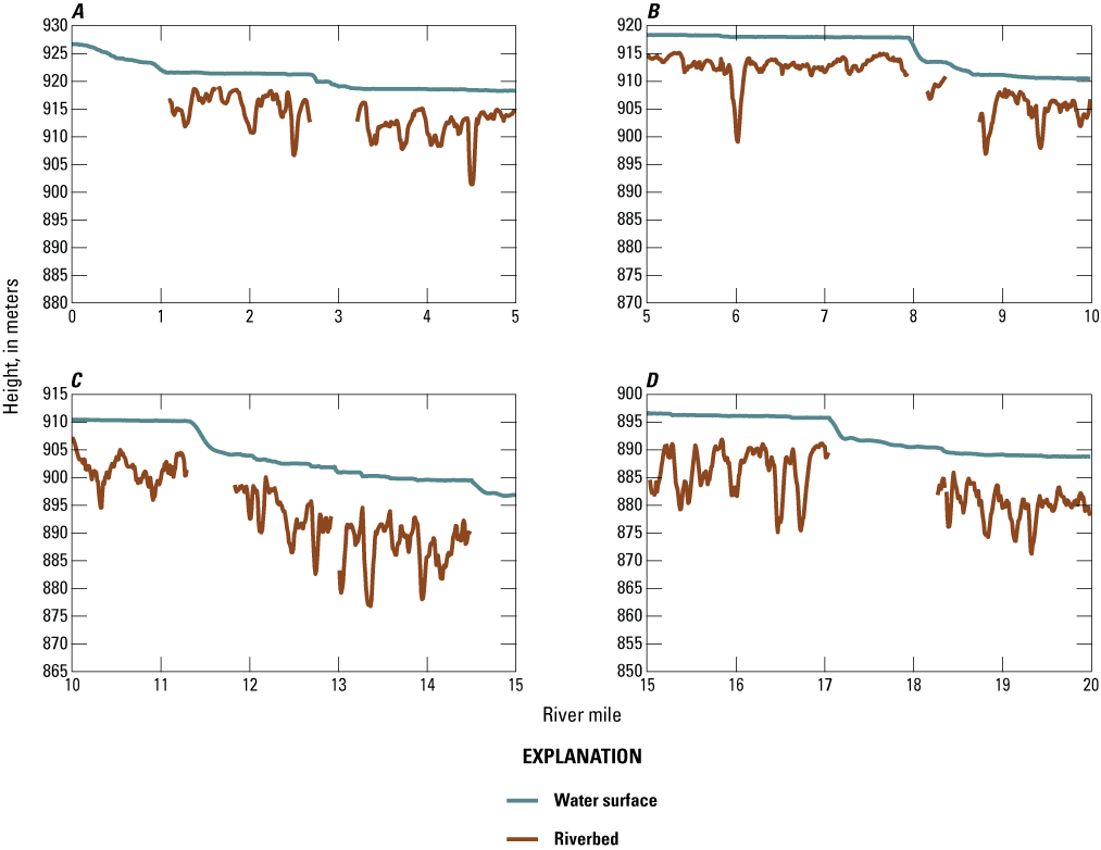
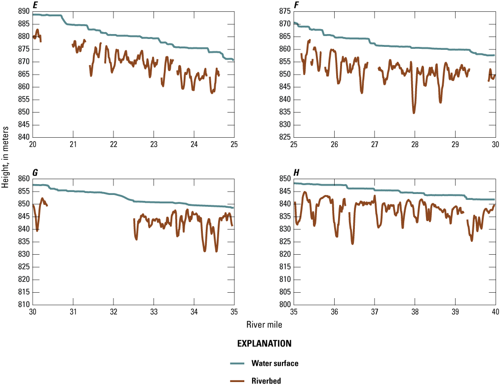
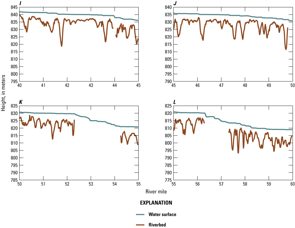
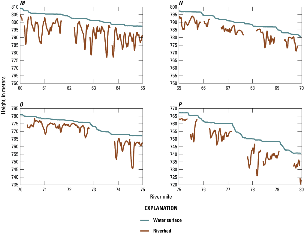
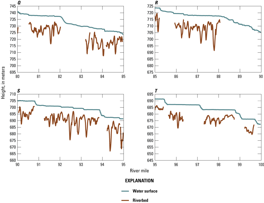
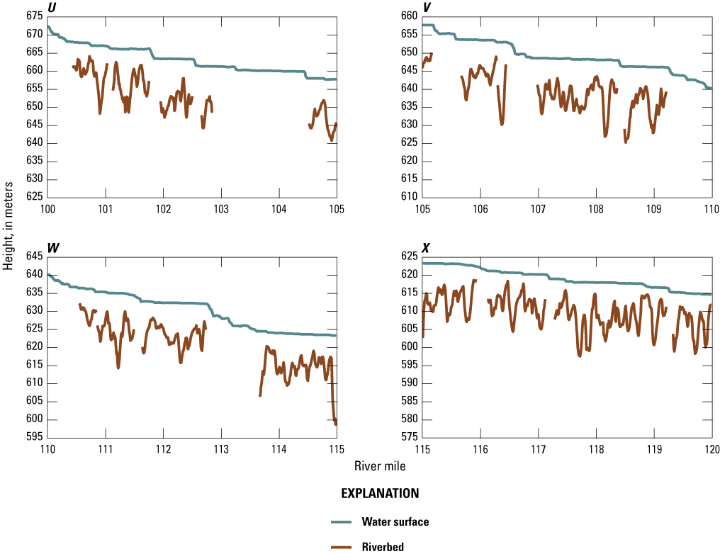
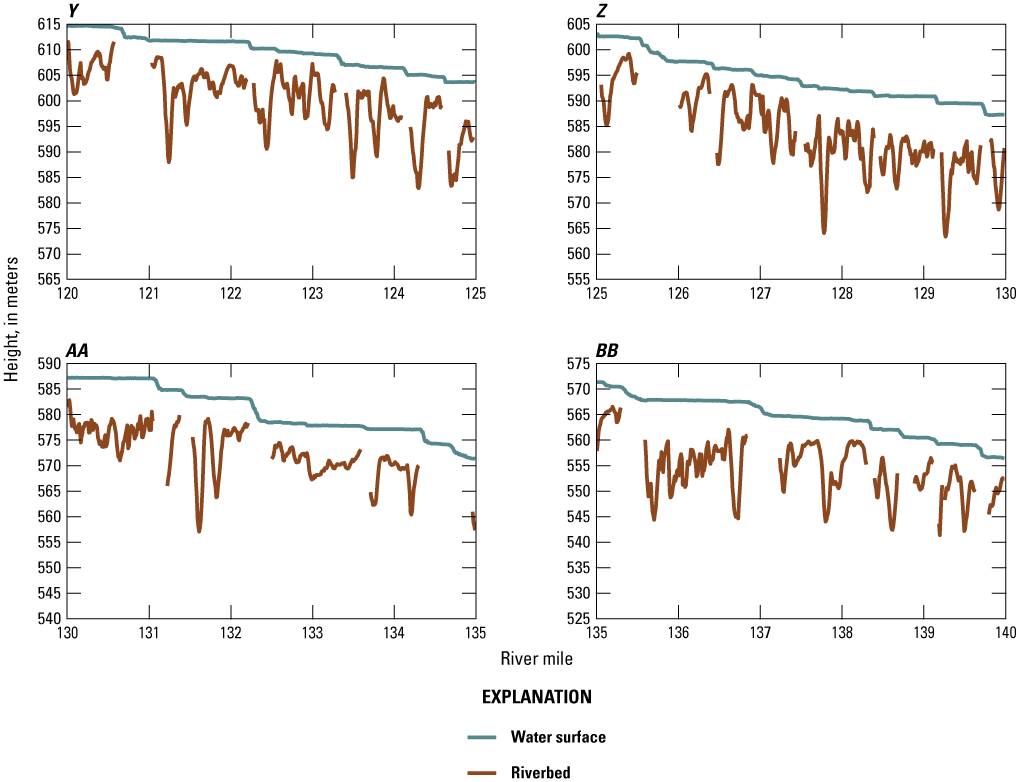
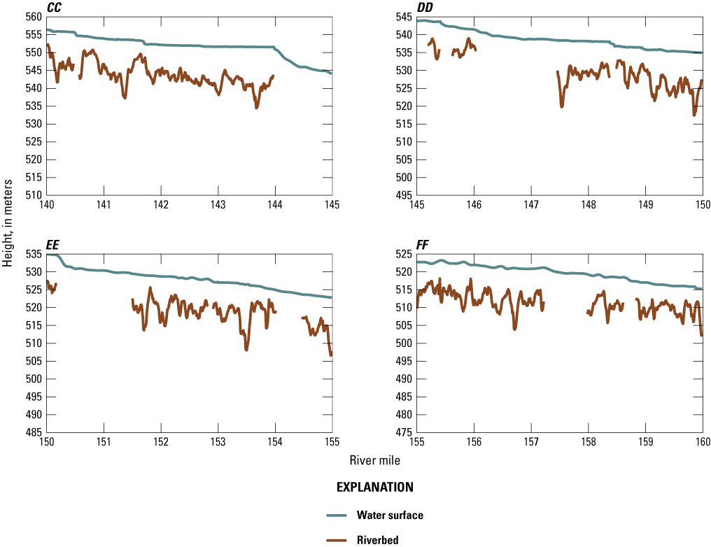
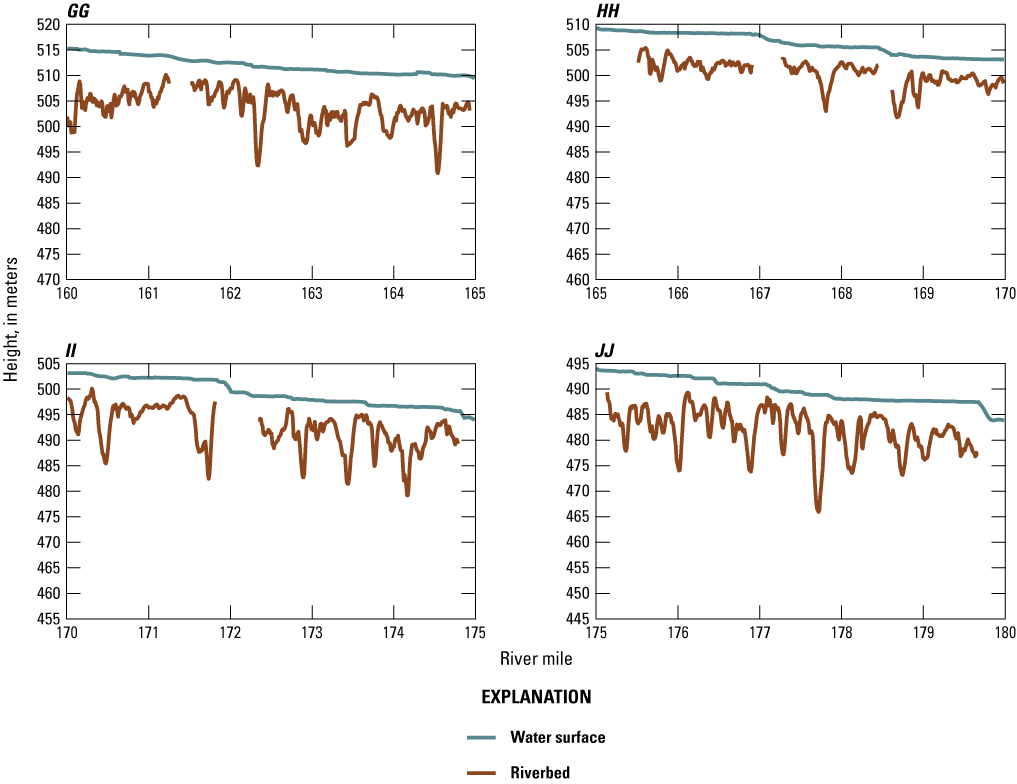
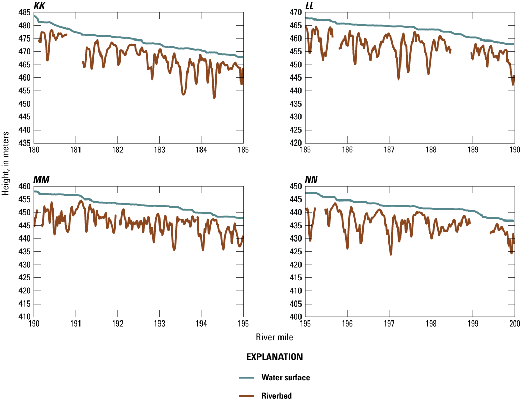
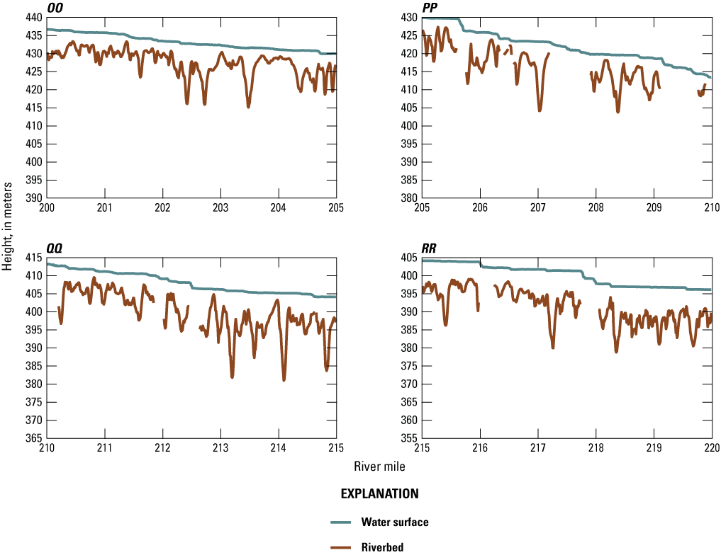
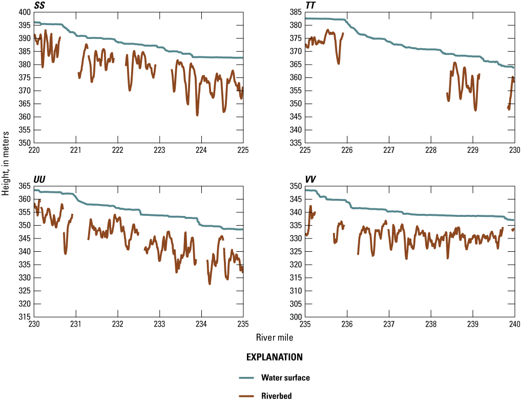
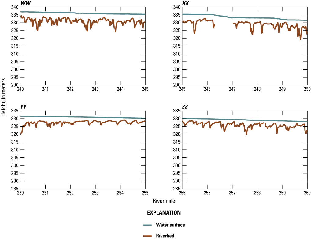
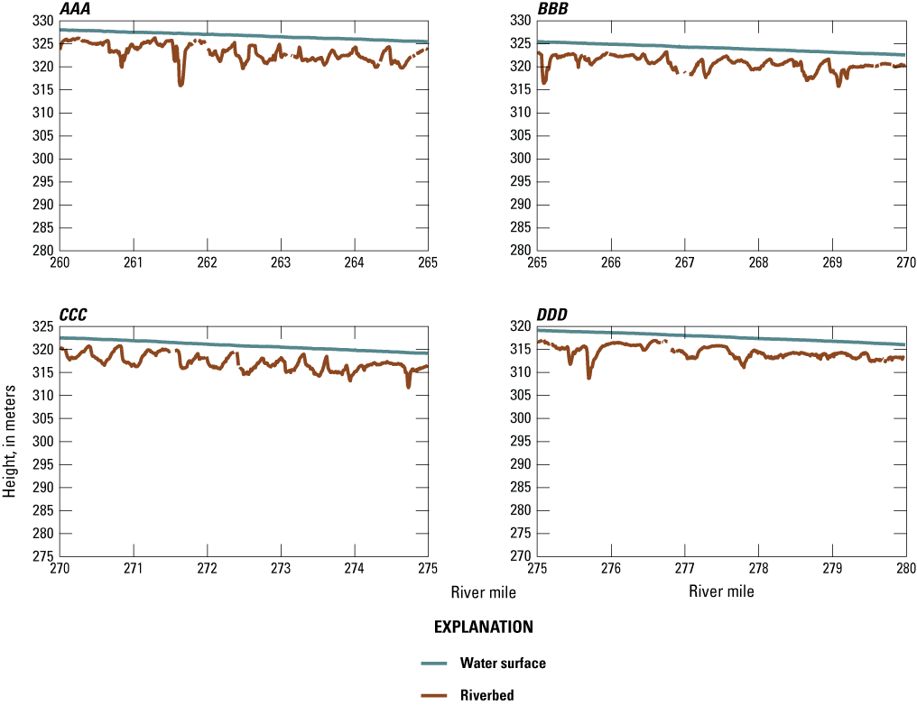
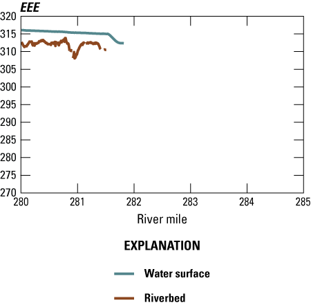
A–EEE, Fifty-seven profiles of water surface and riverbed height from river mile 0 to river mile 282, relative to the Geodetic Reference System 1980 ellipsoid defined by the 2011 adjustment of the North American Datum of 1983. In each profile, riverbed bathymetry represents the 1st percentile (approximately the minimum) of the elevation of each river hundredth mile. Gaps in the riverbed profile correspond to decreases in water surface elevation at rapids where riverbed elevations could not be measured.
Conversion Factors
Datums
Vertical coordinate information and height as used in this report is referenced to the Geodetic Reference System 1980 ellipsoid defined by the 2011 adjustment of the North American Datum of 1983 (NAD 83 [2011]). Where water surface elevation slope was calculated, orthometric heights were computed in the North American Vertical Datum of 1988 (NAVD 88) via Geoid18 (Federal Geodetic Control Subcommittee, 1993). Where historical water surface elevations were used, they were converted from the National Geodetic Vertical Datum of 1929 to ellipsoid heights relative to NAD 83 (2011).
Horizontal coordinate information is referenced to NAD 83 (2011) and projected to the State Plane Coordinate System of 1983, Arizona central zone, in meters.
Abbreviations
CORS
Continuously Operating Reference Stations
DEM
digital elevation model
DSM
digital surface model
GCSRN
Grand Canyon Spatial Reference Network
GNSS
global navigation satellite system
INS
inertial navigation system
lidar
light detection and ranging
MBES
multibeam echosounder
NGS
National Geodetic Survey
NSRS
National Spatial Reference System
PPK
postprocessed kinematic
RM
river mile
RMSE
root mean square error
SBET
smoothed best estimate of trajectory
VBS
virtual base station
For more information about this report, contact:
Director, Southwest Biological Science Center
U.S. Geological Survey
2255 N. Gemini Drive, Flagstaff, AZ 86001
https://www.usgs.gov/centers/southwest-biological-science-center
Publishing support provided by the USGS Science Publishing Network, Lafayette, Moffett Field, and Pembroke Publishing Service Centers
Disclaimers
Any use of trade, firm, or product names is for descriptive purposes only and does not imply endorsement by the U.S. Government.
Although this information product, for the most part, is in the public domain, it also may contain copyrighted materials as noted in the text. Permission to reproduce copyrighted items must be secured from the copyright owner.
Suggested Citation
Sartain, S.L., Kaplinski, M.A., Kohl, K., Chapman, K.A., Bransky, N.D., Sankey, J.B., and Grams, P.E., 2026, Continuous and high-resolution longitudinal profiles of the water surface and riverbed elevation for 282 miles of the Colorado River from Lees Ferry to Pearce Ferry, Arizona, 2021: U.S. Geological Survey Scientific Investigations Report 2026–5010, 40 p., https://doi.org/10.3133/sir20265010.
ISSN: 2328-0328 (online)
Study Area
| Publication type | Report |
|---|---|
| Publication Subtype | USGS Numbered Series |
| Title | Continuous and high-resolution longitudinal profiles of the water surface and riverbed elevation for 282 miles of the Colorado River from Lees Ferry to Pearce Ferry, Arizona, 2021 |
| Series title | Scientific Investigations Report |
| Series number | 2026-5010 |
| DOI | 10.3133/sir20265010 |
| Publication Date | May 26, 2026 |
| Year Published | 2026 |
| Language | English |
| Publisher | U.S. Geological Survey |
| Publisher location | Reston, VA |
| Contributing office(s) | Southwest Biological Science Center |
| Description | Report: vii, 40 p.; Data Release |
| Country | United States |
| State | Arizona |
| Other Geospatial | Colorado River |
| Online Only (Y/N) | Y |
| Additional Online Files (Y/N) | N |