Scientific Investigations Report 2006-5035
U.S. GEOLOGICAL SURVEY
Scientific Investigations Report 2006-5035
Because gaging stations cannot be located at all sites where streamflow information is needed, other methods are used to estimate streamflow statistics for these sites. The two most commonly used methods for estimating streamflow statistics at ungaged sites are the drainage-area ratio method and regression equations (Ries and Friesz, 2000). The drainage-area ratio method can be used when the ungaged site is located near a gaging station on the same stream. Regression equations can be used to estimate streamflow statistics at most ungaged sites.
A major assumption of the drainage-area ratio method is that the streamflow at the ungaged site is the same per unit area as the streamflow at a nearby gaging station located on the same stream (index site). The method involves determining the drainage areas for both the ungaged site and the index site. The streamflow statistics are computed for the index site and then are divided by the drainage area to determine the streamflow per unit area for each statistic. The values for streamflow per unit area are then multiplied by the drainage area for the ungaged site to estimate the statistics for that site. The accuracy of this method depends on the proximity of the two sites and the similarities in drainage area and other physical and climatic (basin) characteristics of their drainage basins. The equation that represents this method is as follows:
 , (1)
, (1)
where

|
is the streamflow statistic for the ungaged site, |

|
is the drainage area for the ungaged site, |

|
is the drainage area for the gaged site, and |

|
is the streamflow statistic for the gaged site. |
It is fairly common practice to use this method when the sites are located on the same stream and the ratio between the drainage areas of the index site and the ungaged site is between 0.5 and 1.5. On the basis of specific analyses in certain areas, some researchers have found that this range should be either reduced or expanded. Koltun and Schwartz (1986) recommended a range of 0.85 to 1.15 times the area of the index site for estimates of low-flow statistics in Ohio, and Ries and Friesz (2000) determined that a range of 0.3 to 1.5 was applicable for low-flow statistics in Massachusetts. Parrett and Johnson (2004) recommended the standard ratio of 0.5 to 1.5 for flood frequency analyses in Montana, as did Berenbrock (2002) and Kjelstrom (1998) for flood-frequency analyses in Idaho.
The regression analyses were completed for eight separate geographic regions of the State, as was done in the recent peak-flow and monthly exceedance studies (Hortness and Berenbrock, 2001 and 2003; Berenbrock, 2002). Basin and climatic variables (basin characteristics) for the gaging stations used in this study were obtained from previous studies or determined using GIS algorithms equivalent to those used in previous studies. Two types of regression analyses, logistic and multiple linear, were used. Logistic regression analysis was used for regions that included gaging stations at which any of the relevant N-day low flows equaled zero. Data from those stations were used to develop an equation for use in determining the probability of the annual minimum N-day flow being zero for an ungaged site. Multiple linear regression analyses were used in all regions to develop equations for estimating low-flow frequency statistics.
The regional boundaries used in this study are the same ones that were defined by Hortness and Berenbrock (2001): eight study regions and one undefined region that was not included in the analysis (fig. 1). The region boundaries were determined on the basis of the following: (1) grouping of gages with similar basin characteristics revealed during cluster analyses (statistical method for grouping data with similar characteristics), (2) location of geographic features, such as large mountain ranges or breaks between mountains and plains, and (3) use of hydrologic judgment based on general knowledge of the area. The undefined region is made up almost entirely of the area commonly referred to as the eastern Snake River Plain. This area includes several dams, major irrigation diversions, springs with extremely large discharges, and flat-land drainages and channel bottoms with very high infiltration rates. This area was not included in the analysis because flows influenced by these conditions cannot be characterized by a regional regression approach. More detailed information on how the regional boundaries were determined can be found in the previous report by Hortness and Berenbrock (2001).
More than 30 separate basin characteristics were obtained for each of the 234 gaging stations included in this study. The basin characteristics for gaging stations included in previous studies by Hortness and Berenbrock (2001; 2003) and Berenbrock (2002) were used in this study. For gaging stations not included in those studies, the basin characteristics were derived using current GIS techniques equivalent to those used in the previous studies. In general, all basin characteristics were obtained using either custom Arc Macro Language (AML) programs written for ArcGIS or current tools (ArcHydro Tools) available in ArcGIS version 9.0 (Environmental Systems Research Institute, Inc., 2005). The sources for the values of all basin characteristics are given in table 1 and a list of all basin characteristics considered during this study are presented in table 8 (at back of report).
Several basin characteristics were removed from consideration after a review of the correlation plots of the data. Generally, if two basin characteristics correlated well with each other, the one that was the least difficult to obtain was kept and the other was removed. Other characteristics were removed because of missing data or difficulty in obtaining the data. Descriptions of the basin characteristics used in the final equations and the methods of determination are provided in table 2, and basin-characteristic values for each gaging station are listed in table 9 (at back of report).
| Dataset | Source |
|---|---|
| National Elevation Dataset (NED) | Several basin characteristics were calculated using 30-meter-resolution digital-elevation data derived from the 1-arc-second National Elevation Dataset (NED) (URL: http://ned.usgs.gov/). |
| Elevation Derivatives for National Applications (EDNA) | Hydrologic derivatives of NED data were developed using procedures similar to those of EDNA Stage 1 processing, using a custom projection for Idaho (URL: http://edna.usgs.gov/Edna/methodology.asp). |
| National Land Cover Dataset (NLCD) | Vogelmann, J.E., Sohl, T.L., Campbell, P.V., and Shaw, D.M., 1998, Regional land-cover characterization using Landsat Thematic Mapper data and ancillary data sources: Environmental Monitoring and Assessment v. 51, p. 415-428 (URL: http://landcover.usgs.gov/natllandcover.asp). |
| Major lithology, Pacific Northwest | U.S. Geological Survey, 1995, Major lithology: Spokane, Washington, U.S. Geological Survey, polygon data converted to grid-cell resolution 200 meters (URL: http://www.icbemp.gov/spatial/min). |
| Mean annual precipitation, Idaho(used for areas within Idaho) | Molnau, M., 1995, Mean annual precipitation, 1961-1990, Idaho: Moscow, University of Idaho, Agricultural Engineering Department, State Climate Program, scale 1:1,000,000 (URL: http://snow.ag.uidaho.edu/Climate/reports.html). |
| Western United States average monthly or annual precipitation(PRISM; used for areas outside of Idaho) | Daly, C., and Taylor, G., 1998, Western United States average monthly or annual precipitation, 1961-90, Oregon: Portland, Water and Climate Center of the Natural Resources Conservation Service, grid-cell resolution 4 kilometers (URL: http://www.ocs.orst.edu/prism/prism_new.html). |
| Basin characteristic(identifier) | Description |
|---|---|
| Drainage area (A) | Drainage area of the basin that contributes surface runoff, in square miles; estimated using Arc/Info Grid with 30-meter-resolution digital-elevation models (DEMs). |
| Mean annual precipitation (P) | Mean annual precipitation over the entire drainage area, in inches; estimated using Arc/Info Grid with a combination of 500-meter resolution (within Idaho) and 4-kilometer resolution (outside of Idaho) precipitation grids covering the 1961-1990 period. |
| Developed land (DV) | Areas of residential, commercial, industrial, and transportation lands, in percentage of drainage area; estimated from the National Land Cover Dataset (NLCD) 1992 version. |
| Agricultural land (AG) | Areas of pasture, row crop, small grain, fallow, and urban/recreational grass lands, in percentage of drainage area; estimated from the National Land Cover Dataset (NLCD) 1992 version. |
| Basin slope (BS) | Average slope of the basin, in percent; estimated using the SLOPE function in Arc/Info Grid with 30-meter-resolution DEMs. |
| Water (W) | Areas of open water or perennial ice and snow, in percentage of drainage area; estimated from the National Land Cover Dataset (NLCD) 1992 version. |
| Basin relief (R) | Relief of the basin, in feet; estimated using Arc/Info Grid with 30-meter-resolution digital-elevation models (DEMs). |
| Surficial volcanic rocks (V) | Areas of surficial volcanic rocks, in percentage of drainage area; estimated from the Pacific Northwest Major Lithology data set. |
| Slopes greater than 50 percent (S50) | Area with slopes greater than 50 percent, in percentage of drainage area; estimated using the SLOPE function in Arc/Info Grid with 30-meter-resolution DEMs. |
Logistic regression analyses were used to develop equations that relate the probability of a specific N-day low flow equaling zero to basin characteristics. The use of logistic regressions for water-resources applications is discussed in more detail by Helsel and Hirsch (1992). Applications specific to low-flow analyses can be found in a paper by Tasker (1989) and a report by Ludwig and Tasker (1993). Hosmer and Lemeshow (2000) provide a complete discussion of logistic regression.
The output variable in a logistic regression equation is dichotomous (binary), meaning that there are two possible outcomes. In this study, the possible outcomes were flow or no flow. Logistic regression is conceptually similar to multiple linear regression because the relation between one dependent variable and several independent variables is evaluated. The differences are reflected in the form of the equation and in the assumptions. Four important concepts regarding logistic regression analyses are as follows: (1) the conditional mean of the regression equation must fall between zero and 1; (2) the distribution of the errors is binomial, not normal; (3) equation coefficients are estimated using the log likelihood function, not least squares as is done in linear regression; and (4) the general principles that guide the development of linear regression equations are also relevant for logistic regression (Hosmer and Lemeshow, 2000).
The final form of the logistic regression equation results in a probability of success of one of the two possible outcomes. For this study, it was the probability that the specific N-day low flow is equal to zero. The final form of the logistic regression equation can be written as follows:
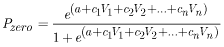 , (2)
, (2)
where

|
is the probability of the N-day low flow being equal to zero, |

|
is the regession model constant, |

|
is a mathematical constant, |

|
are the regression model coefficients, and |

|
are the required basin characteristics. |
Data from each of the gaging stations listed in table 6 were used in the logistic regression analyses. The Statit Custom QC (Statit Software, 2005) statistical software package was used to perform the logistic regression analyses. The data required to perform the analyses included the total number of years of record, total number of years that each of the specific N-day low flows equaled zero, and basin characteristics for each gaging station in the region being analyzed. In the analyses, the number of years that the specific N-day low-flow equaled zero was the dependent variable, the total number of years of record was the binomial trials variable (number of possible zero-flow years), and the basin characteristics were the independent variables. The total years of N-day zero flows and total years of record for each of the gaging stations are presented in table 10 (at back of report). Only region 2 had no gaging stations with at least 1 year where one of the N-day low flows equaled zero. Basin‑characteristic data for the gaging stations were presented previously in table 9.
Several statistical parameters were used to help with the selection of the final probability equations. The overall likelihood ratio tests whether the model coefficients are significantly different from zero. This ratio follows a chi‑squared distribution and computed p-values indicate whether model coefficients are significantly different from zero. A p-value threshold of 0.05 was used for this analysis. McFadden’s R2 is a transformation of the log-likelihood ratio intended to be similar to the unadjusted R2 in linear regression. However, McFadden’s R2 tends to be smaller than R2 in linear regression. The percentage of correct responses is calculated as the number of observed zero flows that were predicted by the model as zero flows, plus the number of non-zero flows predicted by the model as non-zero flows, divided by the total number of gaging stations used in the analysis. The odds ratio is a measure of the relative influence of an independent variable on the model.
The use of multiple linear regression equations is the most common method used for estimating streamflow statistics at ungaged sites. In multiple linear regression analyses, streamflow statistics from several long-term gaging stations are statistically related to various basin characteristics for each of the gaging stations. The resulting equation can then be used with the relevant basin characteristics to estimate streamflow statistics at ungaged sites where no streamflow data are available.
The typical form of equations generated from multiple linear regression analyses is
 , (3)
, (3)
where

|
is the estimate of the dependent variable for site |

|
are the |

|
are the |

|
is the residual error (difference between the observed and estimated values of the dependent variable) for site |
Four assumptions are associated with the regression analyses: (1) the mean of![]() is zero, (2) the variance of
is zero, (2) the variance of ![]() is constant and independent of the values of
is constant and independent of the values of![]() , (3) the values for
, (3) the values for![]() are normally distributed, and (4) the values for
are normally distributed, and (4) the values for![]() are independent of each other (Haan, 1977).
are independent of each other (Haan, 1977).
Streamflow statistics and basin characteristics generally are log-normally distributed. As a result, a log transformation of the variables is necessary to satisfy assumption 1 above. The use of log-transformed values results in an equation of the following linear form:
 . (4)
. (4)
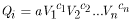
The coefficients for this equation are derived from the multiple linear regression analyses and then the equation is transformed back to original units. The retransformed equation takes on the following form:
 . (5)
. (5)
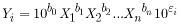
In hydrologic terms, assuming that![]() is zero as stated in the assumptions above, the equation can be written as:
is zero as stated in the assumptions above, the equation can be written as:
 , (6)
, (6)
where

|
is the low-flow statistic, |

|
is the model constant transformed back to original units, |

|
are the required basin characteristics, and |

|
are the regression model coefficients. |
Because streamflow data are essentially correlated spatially and in time, assumption 4 is not strictly satisfied when the most commonly used form of regression analysis, Ordinary Least Squares (OLS) is used. As a result, Generalized Least Squares (GLS) regression techniques were developed for use in regression analysis of peak- and low-flow frequency statistics. GLS techniques are the most appropriate for dealing with hydrologic regressions because the algorithms allow for the weighting of station data to compensate for spatial correlation and differences in record length (Tasker and Stedinger, 1989). For this study, OLS techniques were used to narrow down the list of possible explanatory variables (basin characteristics) and then GLS techniques were used to determine the final estimating equations. The Statit Custom QC (Statit Software, 2005) statistical software package was used to perform the initial regressions using OLS techniques and the USGS software package GLSNET (U.S. Geological Survey, 1998) was used to finalize the equations using GLS techniques.
Because the regression technique for low-flow statistics requires a log transformation, zero values cannot be used in the multiple linear regression analyses. All gaging stations listed in table 6 were used in the analyses except those with specific low-flow statistics equal to zero (see table 7). Depending on the values of the various low-flow statistics for a specific gaging station, it would be possible to include the gaging station in the analysis for one statistic but exclude it from the analysis for another. The basin characteristic values used in the analyses were presented previously in table 8. To ensure that zero values, which cannot be transformed, would not result for any gaging station, 1 percent was added to the values of the following basin characteristics prior to the log transformation: developed land (DV), agricultural land (AG), water (W), volcanic rock (V), and slopes greater than 50 percent (S50). In addition, basin relief (R) was divided by 1,000 prior to transformation to allow for more convenient coefficients in the final equations.
The final equations were chosen primarily, but not exclusively, on the basis of the following statistical parameters: (1) mean square error (MSE), the model error variance of the estimates for the stations included in the analysis; (2) R2adj, the percentage of the variation in the dependent variable explained by the independent variables, adjusted for the number of stations and the number of independent variables used in the regression analysis; and (3) the PRESS statistic, an estimate of the prediction error sum of squares. In the end, simpler equations were chosen over more complex equations if the statistical parameters were similar.
Logistic regression analyses were performed for each of the regions with at least one gaging station with N-day low‑flow data equal to zero (all the regions except region 2). The analyses in three of those regions—4, 6, and 7—resulted in equations that were statistically significant for estimating the annual probability of zero flows for 1-, 7-, and 30-day periods. Likely reasons why statistically significant equations could not be developed for regions 1, 3, 5, and 8 are that there were a relatively small number of gaging stations with N-day low-flow values equal to zero or there were a small number of zero values per gaging station.
The logistic regression equations developed for regions 4, 6, and 7 are presented in table 3 and should be used to determine the probability of the specific annual minimum N-day flows equaling zero for ungaged sites in those regions before low-flow frequency statistics are estimated. Values for some of the previously defined statistical parameters used to evaluate the quality of the equations are included in table 3. If the resulting probability is greater than the non-exceedance probability for the statistic of interest, then the expected value for that statistic would be zero and the low-flow frequency equations should not be used. If the resulting probability is less than the non-exceedance probability for the statistic of interest, then the low-flow frequency equations should be used to estimate the value of the statistic. For example, if the probability of a specific 7-day low flow equaling zero was 0.35 from the equation, the expected value for the 7Q10 statistic would be zero (0.35 > 0.10 or 1/10), and the expected value for the 7Q2 statistic would be greater than zero (0.35 < 0.50 or 1/2) and should be estimated using the low‑flow frequency equation.
[Locations of regions are shown in figure 1. Zero flow annual probability equation: Pn-day, annual probability of zero flow for n days; A, drainage area in square miles; P, mean annual precipitation, in inches; DV, developed land in percentage of drainage area; AG, agricultural land in percentage of drainage area; BS, basin slope in percent. OLR: Overall likelihood ratio. OLR-p: chi-square p-value for the overall likelihood ratio. Percentage correctly estimated: Based only on the sample data used to develop the equation]
| Zero flow annual probability equation | McFadden’s R 2 | OLR | OLR-p | Percentage correctly estimated | ||
|---|---|---|---|---|---|---|
| Region 4 | ||||||
| P1-day = | e(–47.5 – 0.0264A – 0.243P + 50.5(DV+1)) | 0.757 | 148.3 | <0.0001 | 90 | |
| 1 + e(–47.5 – 0.0264A – 0.243P + 50.5(DV+1)) | ||||||
| P7-day = | e(–50.3 – 0.0323A – 0.224P + 52.5(DV+1)) | .717 | 125.1 | <.0001 | 95 | (10-year) |
| 1 + e(-50.3 – 0.0323A – 0.224P + 52.5(DV+1)) | 100 | (2-year) | ||||
| P30-day = | e(–57.1 – 0.0369A – 0.246P + 59.5(DV+1)) | .772 | 127.4 | <.0001 | 100 | |
| 1 + e(–57.1 – 0.0369A – 0.246P + 59.5(DV+1)) | ||||||
| Region 6 | ||||||
| P1-day = | e(25.5 – 0.0160A – 1.29P + 0.908(AG+1)) | 0.847 | 353.2 | <0.0001 | 100 | |
| 1 + e (25.5 – 0.0160A – 1.29P + 0.908(AG+1)) | ||||||
| P7-day = | e(25.0 – 0.0156A – 1.27P + 0.899(AG+1)) | .828 | 338.8 | <.0001 | 96 | (10-year) |
| 1 + e(25.0 – 0.0156A – 1.27P + 0.899(AG+1)) | 92 | (2-year) | ||||
| P30-day = | e(26.8 – 0.0157A – 1.39P + 0.932(AG+1)) | .809 | 285.9 | <.0001 | 96 | |
| 1 + e(26.8 - 0.0157A – 1.39P + 0.932(AG+1)) | ||||||
| Region 7 | ||||||
| P1-day = | e(8.39 – 0.0136A – 0.442BS) | 0.537 | 217.1 | <0.0001 | 78 | |
| 1 + e(8.39 – 0.0136A – 0.442BS) | ||||||
| P7-day = | e(8.09 – 0.0121A – 0.454BS) | .547 | 200.3 | <.0001 | 74 | (10-year) |
| 1 + e(8.09 – 0.0121A – 0.454BS) | 96 | (2-year) | ||||
| P30-day = | e(8.92 – 0.0141A – 0.516BS) | .607 | 183.4 | <.0001 | 89 | |
| 1 + e(8.92 – 0.0141A – 0.516BS) | ||||||
[Locations of regions are shown in figure 1. Low-flow frequency equation:A, drainage area, in square miles; BS, basin slope, in percent; P, mean annual precipitation, in inches; R, basin relief, in feet; S50, slopes greater than 50 percent in percentage of drainage area; V, surficial volcanic rocks, in percentage of drainage area; W, water, in percentage of drainage area]
| Low-flow frequency equation | Standard error of model | Standard error of prediction | ||||
|---|---|---|---|---|---|---|
| log10 | Percent | log10 | Percent | |||
| Region 1 | ||||||
| 1Q10 = 0.794 A0.420 (W + 1)1.32 | 0.078 | +19.7 to –16.6 | 0.177 | +50.3 to –33.5 | ||
| 7Q10 = 0.804 A0.453 (W + 1)1.22 | .032 | +7.55 to –7.02 | .155 | +43.0 to –30.1 | ||
| 7Q2 = 0.731 A0.613 (W + 1)0.907 | .032 | +7.55 to –7.02 | .132 | +35.4 to –26.1 | ||
| 30Q5 = 0.911 A0.512 (W + 1)1.05 | .032 | +7.55 to –7.02 | .136 | +36.7 to –26.8 | ||
| Region 2 | ||||||
| 1Q10 = 0.0000497 A1.05P2.03 | 0.333 | +115 to–53.5 | 0.346 | +122 to –54.9 | ||
| 7Q10 = 0.0000728 A1.06P1.98 | .317 | +107 to –51.8 | .329 | +113 to –53.1 | ||
| 7Q2 = 0.000153 A1.04 P1.92 | .243 | +74.9 to –42.8 | .253 | +78.9 to –44.1 | ||
| 30Q5 = 0.000164 A1.04 P1.87 | .270 | +86.3 to –46.3 | .281 | +91.0 to –47.6 | ||
| Region 3 | ||||||
| 1Q10 = 0.00492 A–0.0990 (R/1,000)5.15 | 0.467 | +193 to –65.9 | 0.552 | +257 to –72.0 | ||
| 7Q10 = 0.00964 A–0.0923 (R/1,000)4.76 | .462 | +190 to –65.5 | .545 | +251 to –71.5 | ||
| 7Q2 = 0.00953 A0.392 (R/1,000)3.36 | .298 | +98.6 to –49.6 | .351 | +125 to –55.4 | ||
| 30Q5 = 0.0186 A0.109 (R/1,000)3.84 | .327 | +112 to –52.9 | .386 | +143 to –58.9 | ||
| Region 4 | ||||||
| 1Q10 = 0.00000187 A1.03 P2.90 | 0.452 | +183 to –64.7 | 0.471 | +195 to –66.2 | ||
| 7Q10 = 0.00000222 A1.05P2.88 | .432 | +170 to –63.0 | .449 | +181 to –64.4 | ||
| 7Q2 = 0.0000215 A1.04P2.41 | .328 | +113 to –53.0 | .341 | +119 to –54.4 | ||
| 30Q5 = 0.00000993 A1.04P2.58 | .360 | +129 to –56.4 | .375 | +137 to –57.8 | ||
| Region 5 | ||||||
| 1Q10 = 0.0000497 A0.968 (V+1)1.96 | 0.382 | +141 to –58.5 | 0.419 | +163 to –61.9 | ||
| 7Q10 = 0.0000654 A0.959 (V+1)1.96 | .341 | +120 to –54.4 | .378 | +139 to –58.1 | ||
| 7Q2 = 0.000453 A1.04 (V+1)1.51 | .042 | +10.3 to –9.31 | .103 | +26.9 to –21.2 | ||
| 30Q5 = 0.000190 A0.981 (V+1)1.74 | .222 | +66.6 to –40.0 | .255 | +80.0 to –44.5 | ||
| Region 6 | ||||||
| 1Q10 = 0.0000324 A1.06P2.38 | 0.287 | +93.8 to –48.4 | 0.309 | +104 to –50.9 | ||
| 7Q10 = 0.0000360 A1.06P2.38 | 0.286 | +98.3 to –43.3 | .307 | +103 to –50.7 | ||
| 7Q2 = 0.000133 A1.05P2.10 | 0.226 | +68.5 to –40.6 | .243 | +75.0 to –42.9 | ||
| 30Q5 = 0.000127 A1.04P2.10 | 0.264 | +83.5 to –45.5 | .283 | +91.9 to –47.9 | ||
| Region 7 | ||||||
| 1Q10 = 0.0149 A0.613 (S50 + 1)0.949 | 0.544 | +250 to –71.5 | 0.614 | +311 to –75.7 | ||
| 7Q10 = 0.0177 A0.627 (S50 + 1)0.924 | .503 | +219 to –68.6 | .570 | +271 to –73.1 | ||
| 7Q2 = 0.0329 A0.678 (S50 + 1)0.796 | .483 | +204 to –67.1 | .533 | +241 to –70.7 | ||
| 30Q5 = 0.0272 A0.648 (S50+1)0.851 | .485 | +206 to –67.3 | .541 | +248 to –71.2 | ||
| Region 8 | ||||||
| 1Q10 = 3.15 A0.866BS –0.640 | 0.201 | +59.0 to –37.1 | 0.226 | +68.3 to –40.6 | ||
| 7Q10 = 2.27 A0.903BS –0.545 | .124 | +33.0 to –24.8 | .157 | +43.6 to –30.4 | ||
| 7Q2 = 3.86 A0.930BS –0.648 | .136 | +36.9 to –27.0 | .157 | +43.4 to –30.3 | ||
| 30Q5 = 6.17 A0.940BS –0.844 | .119 | +31.6 to –24.0 | .144 | +39.2 to –28.1 | ||
Although equations were not able to be developed for regions 1, 3, 5, and 8, the data show that it is possible, though not very common, to have occurrences of zero flow at certain locations within these regions. Thus, low-flow estimates approaching zero for ungaged sites (determined from the regression equations) may need additional analyses to determine if zero flows also are likely. Analyses could include comparisons of basin characteristics to gaging stations with known zero-flow occurrences in the same region (table 10) or field observations during expected low-flow periods.
Multiple linear regression analyses resulted in the development of four equations to estimate the low‑flow frequency statistics 1Q10, 7Q2, 7Q10, and 30Q5 for unregulated streams in each of the eight regions in the State. The final equations are presented in table 4, along with the associated standard error of the model and the standard error of prediction for each equation. The standard error of the model measures how well the regression model fits the data used to develop it. The standard error of prediction includes the model error as well as an estimate of the sample error and is a better indicator of the model’s overall predictive ability (Pope and others, 2001). The values presented in log10 format represent the errors of the log-transformed equations. The percentage values represent the range of errors for the final untransformed equations. These values were determined using error transformation equations presented in Riggs (1968).
The percentage of correct values for the zero-flow probability equations ranged from 74 to 100 percent (table 3). The values for regions 4 and 6 were all 90 percent or higher. The values for region 7 ranged from 74 to 96 percent. These values provide an indication of the accuracy of the equations based only on the data used to develop the equations. It is assumed that the data used in each region provide a good representation of the zero-flow characteristics of streams in the region. However, any variability in the zero-flow characteristics within each region that was not represented in the development of the equations may have an effect on the final predictive accuracy of the equations.
The model and prediction standard errors for the final estimating equations range significantly across the eight regions (table 4). Equations for regions 1 and 8 had relatively low standard errors, whereas those for regions 3 and 7 were quite large. The large errors associated with the region 3 equations may be the result of the low number of gaging stations (eight) available for the analysis. The large errors associated with the region 7 equations likely indicate that the available basin characteristics do not adequately represent the factors that affect low flows in this area. The natural variability of streamflow may also be an important factor. Prediction of streamflow statistics that have a high degree of variability will always have more uncertainty than prediction of statistics that are more stable. Hortness and Berenbrock (2001) noted that the natural variability of streamflow in regions 6 and 7 is generally greater than the natural variability in the other regions. It is also important to note that even a large percentage error associated with low-flow values does not necessarily result in a large-magnitude error range around the value. For example, a low-flow value of 5.0 ft3/s with errors of +150 and -75 percent would have a resulting error range of 1.25 to 12.5 ft3/s.
The standard errors of prediction for the equations across the eight regions had a minimum range of +26.9 to -21.2 percent for the 7Q2 statistic in region 5 and a maximum range of +311 to -75.7 percent for the 1Q10 statistic in region 7. These error values represent the general predictive ability of the estimating equations; however, other factors could limit the applicability of the equations. It is important to note that because of the transformation from log to back to arithmetic units, the standard error values will always have larger positive values than negative values.
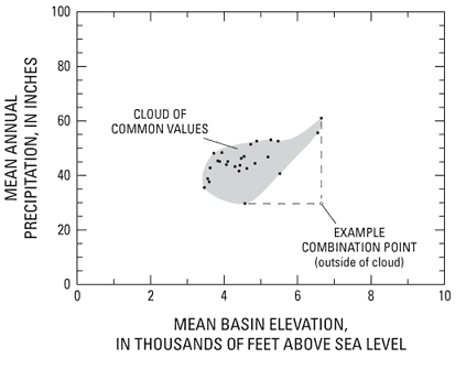
Because the zero-flow probability and low-flow estimating equations are based on regression analyses, the equations might not be reliable for sites where the basin‑characteristic values are outside of the range of values that were used to develop the equations (table 5). In addition, using basin characteristic values near their extremes (maximum or minimum, table 5) might result in unreliable estimates. Figure 2 shows a “cloud of common values” for two basin characteristics. In this example, if the minimum value for mean annual precipitation and the maximum value for mean basin elevation were used, the combination would plot outside of the “cloud of common values,” thus the corresponding equation might result in unreliable estimates. Generating basin-characteristic values by using datasets or processes other than those described in this study also will result in estimates of unknown reliability. The standard errors for each equation are only applicable if the datasets presented in table 1 are used to obtain the required basin characteristics.
The equations are not applicable for stream reaches affected by irrigation diversions and(or) returns, or dams that regulate streamflow. The Boise River downstream from Lucky Peak Lake, the Clearwater River downstream from Dworshak Reservoir, and the entire Snake River in Idaho are examples of stream reaches within the study area for which the estimating equations are not applicable. However, the equations could be used on regulated streams to provide an estimate of natural flow statistics for comparison with the regulated statistics, given that, as previously explained, all of the basin characteristics for the site fall within the ranges of those used to develop the equations.
[Location of regions are shown in figure 1. Equation variables:A, drainage area, in square miles; P, mean annual precipitation, in inches; DV, developed land, in percentage of drainage area; AG, agricultural land, in percentage of drainage area; BS, basin slope, in percent; W, water, in percentage of drainage area; R, basin relief, in feet; V, surficial volcanic rocks, in percentage of drainage area; S50, slopes greater than 50 percent, in percentage of drainage area]
| Equation variables | A | P | DV | AG | BS | W | R | V | S50 |
|---|---|---|---|---|---|---|---|---|---|
| Region 1 | |||||||||
| Maximum | 1,011.0 | 54.3 | 3.59 | 23.2 | 46.4 | 6.69 | 5,866.9 | 27.9 | 41.4 |
| Minimum | 12.5 | 25.1 | .000 | .005 | 12.2 | .004 | 2,230.6 | .000 | 1.04 |
| Region 2 | |||||||||
| Maximum | 2,442.5 | 69.4 | 1.83 | 4.43 | 66.8 | 3.98 | 7,789.6 | 99.9 | 67.4 |
| Minimum | 3.0 | 24.8 | .000 | .000 | 23.8 | .000 | 1,643.9 | .000 | 2.62 |
| Region 3 | |||||||||
| Maximum | 674.9 | 30.1 | 18.6 | 91.6 | 35.4 | 0.258 | 5,098.9 | 92.7 | 27.5 |
| Minimum | 17.6 | 19.3 | .031 | 7.46 | 10.0 | .006 | 1,442.8 | 14.5 | .018 |
| Region 4 | |||||||||
| Maximum | 5,507.9 | 65.6 | 0.126 | 18.4 | 57.2 | 1.04 | 8,364.5 | 100.0 | 63.1 |
| Minimum | 4.0 | 15.9 | .000 | .000 | 18.7 | .000 | 1,821.4 | 18.2 | 1.27 |
| Region 5 | |||||||||
| Maximum | 12,228.0 | 44.5 | 2.21 | 2.44 | 46.7 | 4.37 | 10,701.3 | 100.0 | 46.1 |
| Minimum | 19.3 | 22.4 | .000 | .000 | 20.2 | .002 | 2,743.5 | 27.1 | 3.47 |
| Region 6 | |||||||||
| Maximum | 6,236.7 | 42.3 | 0.385 | 9.27 | 66.2 | 1.19 | 9,419.7 | 93.0 | 77.2 |
| Minimum | 6.4 | 15.3 | .000 | .000 | 8.60 | .000 | 2,395.4 | .000 | 1.36 |
| Region 7 | |||||||||
| Maximum | 535.3 | 29.3 | 0.296 | 28.1 | 35.3 | 0.599 | 5,683.3 | 100.0 | 28.5 |
| Minimum | 7.4 | 12.3 | .000 | .000 | 10.1 | .000 | 1,681.7 | .000 | .189 |
| Region 8 | |||||||||
| Maximum | 874.8 | 56.0 | 0.176 | 70.7 | 53.2 | 3.83 | 6,232.1 | 90.1 | 60.5 |
| Minimum | 6.6 | 14.2 | .000 | .000 | 6.15 | .000 | 1,100.5 | .000 | .002 |
The estimating equations may not be applicable for streams that exhibit significant gains as a result of spring flow or significant losses as a result of channel seepage. The effects of headwater springs and other small springs that are representative of many or all streams in a particular region because of similar geologic conditions likely would be reflected in the equations for that region. The effects of larger springs which significantly affect streamflows likely would not be reflected in the equations. Similarly, the effects of small losses due to channel seepage which are representative of streams in a particular region likely would be reflected in the equations, while the effects of larger losses likely would not. In specific instances, user judgment may be required to decide if the particular ungaged site of interest is affected by factors similar to those that affected the gaging station data used to develop the relevant equations. For example, results for an ungaged site on the Lemhi River near Lemhi in region 6, which has fairly significant and highly variable streamflow gains and losses (Donato, 1998), may be suspect since no mainstem Lemhi River gaging stations were used to develop the equations. However, if a gaging station from the Lemhi River or another river with similar characteristics were included, the equations likely would produce satisfactory results.
Three examples are given for using the equations to estimate low-flow frequency statistics for unregulated streams in Idaho. Example 1 addresses the basic ungaged site with the entire upstream drainage area located within the same region and no zero-flow probabilities, example 2 addresses the situation where zero-flow probability equations are used to estimate the probability of zero flows at a site (regions 4, 6, and 7, only) and example 3 addresses the situation where the drainage area of a specific site encompasses parts of two separate regions.
An estimate of the 7Q2 low-flow statistic is required for a stream location in region 2. The following required basin characteristics were determined for region 2 equations: ![]() , 2180.5 mi2; and
, 2180.5 mi2; and ![]() , 30.2 in. Since region 2 has no zero flow annual probability equations, the user would go directly to the low-flow frequency regression equations. Based on the basin-characteristic values, the estimated 7Q2 statistic can be computed as follows:
, 30.2 in. Since region 2 has no zero flow annual probability equations, the user would go directly to the low-flow frequency regression equations. Based on the basin-characteristic values, the estimated 7Q2 statistic can be computed as follows:
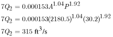
The predicted range of the actual values for this low-flow statistic, based on the range of the standard error of prediction given in table 4, is as follows:
 .
.
An estimate of the 7Q10 low-flow statistic is required for a stream location in region 6. The following required basin characteristics were determined for region 6 equations:![]() , 8.2 mi2; and
, 8.2 mi2; and![]() , 24.7 in.; and
, 24.7 in.; and![]() , 1.35 percent. Based on these values, the probability of the 7-day low-flow equaling zero at this site is computed as follows:
, 1.35 percent. Based on these values, the probability of the 7-day low-flow equaling zero at this site is computed as follows:
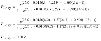 .
.
Because the probability is less than 0.10 (1/10 for 10 year recurrence), the equation estimates that the 7-day low flow for this site is greater than zero. The estimated 7Q10 statistic can then be computed as follows:
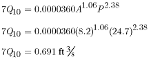 .
.
The predicted range of the actual values for this low-flow statistic, based on the range of the standard error of prediction given in table 4, is as follows:
 .
.
An estimate of the 30Q5 low-flow statistic is required for a site in region 5 on a stream with a drainage basin encompassing parts of regions 5 and 6. The recommended method for handling sites with portions of its drainage basin in two regions is as follows: (1) calculate values for the entire drainage basin by using equations from the first region, (2) calculate values for the entire drainage basin by using equations from the second region, and (3) average the two values on the basis of the proportion of drainage area in each region (Sando, 1998). The following required basin characteristics were determined for region 5 and 6 equations: ![]() , 5,153.0 mi2;
, 5,153.0 mi2; ![]() , 78.5 percent; and
, 78.5 percent; and ![]() , 39.4 in. The portion of the drainage area located in region 5 covers 1,622.0 mi2 and the portion in region 6 covers 3,531.0 mi2. The step to check for the probability of zero flow in region 6 was skipped because of the large portion of the drainage area in region 5. Because the region boundaries were almost exclusively drawn along hydrologic boundaries, the occurrence of zero flows at sites that have portions of the drainage area in two regions is highly unlikely, but should be verified.
, 39.4 in. The portion of the drainage area located in region 5 covers 1,622.0 mi2 and the portion in region 6 covers 3,531.0 mi2. The step to check for the probability of zero flow in region 6 was skipped because of the large portion of the drainage area in region 5. Because the region boundaries were almost exclusively drawn along hydrologic boundaries, the occurrence of zero flows at sites that have portions of the drainage area in two regions is highly unlikely, but should be verified.
Region 5 calculations:
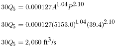 .
.
Region 6 calculations:
.
Area-weighted average:
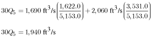 .
.
For more information about USGS activities in Idaho, visit the USGS Idaho Water Science Center home page .

![]() U.S. Department of the Interior |
U.S. Geological Survey
U.S. Department of the Interior |
U.S. Geological Survey
Persistent URL: https://pubs.water.usgs.gov/sir20065035
Page Contact Information: Publications Team
Page Last Modified: Thursday, 01-Dec-2016 18:55:02 EST
