Scientific Investigations Report 2011-5105
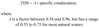
MethodsModel DescriptionThe Link–Keno model was constructed with CE-QUAL-W2 version 3.6 (Cole and Wells, 2008), a two-dimensional, laterally averaged hydrodynamic and water-quality model from the U.S. Army Corps of Engineers and Portland State University. CE-QUAL-W2 can simulate water level, flow, water velocity, water temperature, ice cover, and many water-quality constituents, including total dissolved solids, dissolved oxygen, pH, nutrients, particulate and dissolved organic matter, and algae. It has been applied successfully to hundreds of rivers, lakes, and reservoirs around the world. At a reach scale, a long, narrow, pooled river is typically a good candidate for a two-dimensional, laterally averaged model. Longitudinal and vertical variations are clearly exhibited in field data and indicate that simulation of longitudinal and vertical differences are useful. Although there are certain areas of the river that exhibit lateral (bank-to-bank) variability, these conditions are generally local in character (Vaughn and Deas, 2006; Sullivan and others, 2009). This does not preclude the importance of lateral variability, but on a reach scale (versus a local scale), the CE-QUAL-W2 model was deemed appropriate. The Link–Keno model was developed in several steps. First, a model grid was constructed to represent the course and morphology of the reach. Subsequently, necessary data were collected and formatted to provide meteorological, hydrological, and water temperature and water-quality boundary conditions. Prior to model calibration, representative values for many parameters (for example, rate constants, coefficients, stoichiometric ratios, and so forth) were defined through data derivations, results from experimental work, or from the literature. The water budget for the Link–Keno reach was calibrated by comparing measured and modeled water levels to estimate the gains or losses of water from ungaged inflows, outflows, and groundwater interactions. Water temperature and water-quality constituents were calibrated by comparing measured data at multiple locations throughout the reach to model predictions at the same date, time, and location. The model was initially calibrated for April through November 2007 and 2008, as those periods had the most extensive water-quality datasets available. Subsequently, the calibration period was extended to include calendar years 2006–09 to expand the range of hydrologic, water quality, and meteorological conditions that were modeled and to investigate the feasibility of modeling the reach with sparse datasets (2006 and 2009) as opposed to rich datasets (2007 and 2008). The CE-QUAL-W2 model uses a variable time step; for these models, the time step generally was between 50 and 800 seconds. The model was set up to run in Pacific Standard Time (PST). Field data in Pacific Daylight Time (PDT) were converted to PST for model input files; model output files in PST were converted to PDT when necessary for comparison with field calibration data. Model GridA CE-QUAL-W2 model grid is formed from model segments that connect together in the direction of flow. Each segment has layers of defined height that increase in width from the channel bottom to the top of the grid, thus resembling a cross-sectional shape with stacked rectangles. Segments are grouped together into “branches” that define specific river reaches, and branches can be grouped together as “waterbodies” that have similar meteorological conditions. Cross-sectional shapes were extracted from a recent bathymetric survey of this reach (Eilers and Gubala, 2003) to produce the model grid using geographic information system (GIS) software. Segment boundaries were specified to form 102 active segments in the main river reach from Link River to Keno Dam (branch 1, fig. 2) and three segments describing a channel around an island in the Klamath River just upstream of the inflow of the Lost River Diversion Channel (branch 2). Using GIS techniques, 10 equally spaced cross sections were subsampled within the designated segment boundary lines. The extracted cross-sectional shapes were averaged to determine a representative cross section for each model segment, recomputed to determine equivalent cell widths for a model grid with layer boundaries at specified elevations, and finally formatted as a CE-QUAL-W2 bathymetry input file. The model grid then was checked to ensure that layers at the river bottom were not advectively isolated (a minimum of two neighboring active cells are required in each layer to ensure that advective flow can occur) and that layer widths were greater than 5 m as recommended by the CE-QUAL-W2 development team (Cole and Wells, 2008). Adherence to these requirements is necessary to ensure that run times are reasonable and model instabilities are minimized. Segment lengths ranged between 477 and 1,170 ft (145.5 and 356.9 m) and averaged 1,009 ft (307.6 m); layer heights were all set to 2 ft (0.6096 m). A grid with a layer height of 1 ft (0.3048 m) also was tested, but results were not improved and run time was faster with 2-ft layers. The length of branch 1, from the end of Link River to Keno Dam, totaled 19.6 mi (31.5 km). Model DataMeteorologyThe CE-QUAL-W2 model requires several meteorological data types as model input, including air temperature, dewpoint temperature, wind speed, wind direction, cloud cover, solar radiation, precipitation, and the temperature of precipitation. In a preliminary analysis, meteorological datasets were obtained and compared from several local stations: KLMT (Klamath Falls Airport), KFLO (Klamath Falls Agrimet), KENO (Reclamation), and SSH (USGS South Shore of Upper Klamath Lake). Hourly data from KLMT were determined to be representative and used for most required meteorological inputs, except for solar radiation, which was obtained from KFLO. Cloud-cover data were obtained from the KLMT Automated Surface Observing System (ASOS) station and converted to model units. The ASOS laser beam ceilometer measured cloud cover up to 12,000 ft (National Oceanic and Atmospheric Administration, 1998). When the ASOS data reported clouds at multiple elevations, the elevation with the most cloud coverage was used for model input, similar to methods described by the U.S. Environmental Protection Agency (1997). None of the stations measured the temperature of precipitation directly; therefore, the precipitation temperature was assumed to be equal to air temperature when air temperature was above 0 °C. Precipitation temperature was set to 0 °C when air temperature was below 0 °C. Riparian vegetation along this reach was dominated by low growing herbaceous annuals (for example, Scirpus sp.), and woody riparian vegetation was largely absent. Given the width of the river throughout this reach, vegetative riparian shading was deemed negligible and set to zero in the model. Similarly, the Link–Keno reach traverses a nearly flat plain with few nearby hills or mountains to provide any substantive topographic shading; shading from topographic features also was set to zero in the model. HydrologyThe Klamath River begins at the downstream end of Link River, a short distance downstream of Upper Klamath Lake (fig. 1). The inflow from Link River forms the upstream boundary of the model. Streamflow in Link River upstream of the inflow from the Westside Power Canal was measured every 30 minutes by USGS gage 11507500 (fig. 1, table 2). When part of the flow was routed through the Westside Power Canal, those daily flow values, obtained from PacifiCorp, were added to the USGS gaged flows to provide the total Link River inflow to the Klamath River. Several important tributary inflows and withdrawals were included in the model. Tributaries with measured daily flow data included the Klamath Falls WWTP, South Suburban WWTP, and Columbia Forest Products (all three report discharge information to the Oregon Department of Environmental Quality [ODEQ], and the Klamath Straits Drain and Lost River Diversion Channel (measured by Reclamation). Gaged withdrawals from this reach of the Klamath River include the Ady and North Canals, both with daily flow data from Reclamation. Release rates through Keno Dam were derived from 30-minute flow data from USGS gage 11509500, about 1.5 mi downstream of the dam (fig. 1, table 2). Releases occur through three structures: spill gates, sluice conduit, and fish ladder. Accordingly, the model outflow was apportioned into these three outflows at Keno Dam. The sluice conduit and fish ladder flows were about 130 and 70 ft3/s, respectively, whereas the spill gates released additional water when flow was greater than 200 ft3/s (PacifiCorp, 2002). The highest mean flows were from 2006 and the lowest mean flows were from 2009 for the 2006–09 modeling period (table 1). Daily average water-surface elevations measured at Keno Dam were provided by PacifiCorp and were used in the water balance. Water Temperature and Water QualityWater-quality measurements within the reach were made using three methods: (1) continuous monitors that were deployed at a fixed depth (every 30–60 minutes), (2) vertical profile measurements at multiple depths through the water column (weekly), and (3) grab samples at specific locations and depths at regular intervals (weekly, monthly). Continuous Measurements and Vertical ProfilesReclamation staff deployed and maintained 11 water-quality monitors in the Link–Keno reach during 2006–09 (table 2). The monitors provided hourly measurements throughout the year of water temperature, pH, dissolved oxygen, specific conductance, and sensor depth. Monitors were exchanged weekly from April through October with freshly cleaned and calibrated instruments; from November through March, the monitors were exchanged every 2 weeks. Vertical profiles of these parameters and turbidity as well as Secchi depth measurements were collected during site visits. An overlap period was implemented in the spring of 2007, such that when the clean and freshly calibrated instrument was deployed, the original instrument was left in the river for an additional day. This overlap period was useful during processing of the data to assure data continuity during monitor exchange. Monitor data for calendar years 2006–09 were loaded into the USGS National Water Information System (NWIS) database and processed to correct for fouling and instrument drift using USGS protocols and methods (methods modified from Wagner and others, 2006). Water temperature also was measured every 30 minutes at two USGS sites, one in Link River and the other below Keno Dam (table 2). The continuous monitor dataset was extensive, although some minor gaps were present in the dataset as a result of site visits, probe malfunction, or biological interference (such as snails getting into the conductance probes). For the purpose of creating model boundary inputs, short gaps in the data on the order of a few hours were filled by linear interpolation using data before and after the gap. (The original corrected datasets in NWIS were not modified in this manner.) Longer data gaps, on the order of several days to a week, were filled by comparing (through plots and regressions) daily and seasonal patterns from existing datasets, then choosing an appropriate gap-filling method. For example, linear regression between measured values on each end of a gap could be used when little daily variation was noted for a constituent at a site or time period. However, summer water temperature and dissolved oxygen had strong daily cycles that required other gap-filling methods. Those gaps were filled either by using data directly from a nearby site when justified by close proximity (for example, water temperature gaps at site 11507501 were filled with hourly measurements from site 11507500, or by using modified data from a nearby site with similar cycles, shifted up or down if necessary to smoothly fill the gap. The continuous monitor at the Lost River Diversion Channel began operation in early April 2007; therefore, estimates for water temperature, dissolved oxygen, and specific conductance for this site are more uncertain for January 2006 through March 2007. For the model boundary condition inputs prior to April 2007, water temperature at Lost River Diversion Channel was estimated by using measured temperature from the Klamath Straits Drain for periods when water temperature was less than 10 °C, and from Link River for periods when water temperature was greater than 10 °C. Lost River Diversion Channel specific conductance was dependent on whether flow was to or from the Klamath River, so longer data gaps were filled by assigning a specific conductance of 123 µS/cm for periods when flow was from the Klamath River and a value of 362 µS/cm for periods when flow was to the Klamath River. Dissolved-oxygen concentrations in Lost River Diversion Channel were estimated using several point measurements from upstream in the Lost River at Wilson Reservoir, and then incorporating and shifting dissolved-oxygen data from other sites with a similar magnitude of daily concentration cycles. Grab SamplesExtensive monitoring of water quality with grab samples was conducted as part of the study from April through November of 2007 and 2008. Samples were collected weekly at five mainstem sites and from major tributaries. These intensive sites are designated as both USGS and Reclamation in table 3. Samples were analyzed for total nitrogen and phosphorus; particulate carbon and nitrogen; filtered orthophosphate, nitrite, nitrite plus nitrate, ammonia, and organic carbon; and the enumeration and species identification of phytoplankton and zooplankton. Methods and results for this data-collection effort were documented by Sullivan and others (2008, 2009). More limited pilot sampling also was conducted in late August to early September 2006. Water-quality data for the releases from the Klamath Falls and South Suburban WWTPs and from Columbia Forest Products were obtained from discharge monitoring reports (DMR) provided to ODEQ. Alkalinity was not measured at any of the point sources; it was estimated to be equal to the alkalinity in Link River. Other datasets were required to construct model boundary conditions and calibration datasets for time periods outside of the intensive sampling efforts in 2007 and 2008 (January 2006–March 2007, December 2007–March 2008, and December 2008–December 2009). Water-quality data from Reclamation, ODEQ, and PacifiCorp were obtained and compiled to fill these gaps (table 3). If multiple sources of data were available for a site, the results were plotted together and examined. If the data from one source had notably different concentrations or temporal patterns than data from other sources for the same time and location, this difference was investigated further. If a sampling problem was documented or if no quality-assurance or quality-control data were available, the data were not used for this study. Some of the grab sample data had been censored (presented as less than a reporting level), and special methods were used to address the issues associated with these data. Laboratories usually do not report raw results if the values are below a certain reporting level; instead, that result is simply reported to be less than the reporting level. Although such procedures are useful for avoiding certain types of errors, an uncensored value is required for model input. The raw (uncensored) laboratory data were obtained and used to create the model input file for periods with data from the USGS National Water Quality Laboratory (April–November 2007 and 2008), when data were censored at the reporting level. Values from other agencies reported as less than the reporting level were set to one-half of the reporting level. Acoustic Doppler Current Profiler DataMeasurements of water velocity (speed and direction) were made with acoustic Doppler current profilers (ADCPs) at multiple sites in the Link–Keno reach and as part of an intensive examination of circulation patterns in the Lake Ewauna reach of the Klamath River. An ADCP transmits a fixed frequency sound pulse and measures the frequency shift of acoustic echoes of suspended particles. A series of cross-sectional measurements at selected locations between Link River and Keno Dam were completed using an ADCP from a moving boat on May 30 and September 29, 2007. These measurements included data from most of the cross-sectional area, although a portion near the riverbanks was not measurable because of minimum depth requirements. Portions near the surface and bottom of the water column were not measurable due to the ADCP depth into the water column, blanking distance (a blind zone immediately beneath the ADCP), and interference near the river bottom. Methods and complete results for the cross-sectional work were documented by Sullivan and others (2008). ADCPs were fixed on the river bottom in 2008 and oriented vertically at three sites to measure water velocity profiles continuously from summer through fall. Similar to the cross-sectional work, a portion near the surface and bottom of the water column could not be measured due to signal interference near the water surface, blanking distance, and the height of the instrument mount above the river bottom. One ADCP was deployed on the river bottom at Keno from June 5 through December 7, 2008. That instrument (Argonaut-XR) used three acoustic beams equally spaced at 120°, with each beam 25° from the vertical instrument axis. Water velocity (speed and direction) through the water column was measured every 30 minutes from June 5 to September 23 and every 10 minutes from September 23 to December 7. Water speed and direction data were processed and lumped into four layers of the water column, each 1.4 ft (0.43 m) high. Two other ADCPs (EWA1, EWA2) were deployed in Lake Ewauna from June 4 through October 10, 2008. Those instruments (1,200 kHz Teledyne RD Workhorse) used four acoustic beams equally spaced at 90°, with each beam 20° from the vertical instrument axis. Velocity through the water column was measured every 30 minutes at both Lake Ewauna sites. The morphology of Lake Ewauna is variable, with a relatively deep channel to the west and a wide, shallow area to the east. Thus, the ADCP on the west (EWA1) measured velocity in a deeper water column, usually with 11 data “bins” with a height of 0.7 ft (0.2 m). The ADCP deployed to the east (EWA2) was in the shallow area, resulting typically in three data bins with a height of 0.7 ft. Measured directions for all velocity data were corrected for magnetic declination and are reported relative to true north. Model DevelopmentWater BalanceResults from initial model runs that included precipitation, evaporation, and measured inflows and outflows identified differences between modeled and measured water-surface elevations. This typically occurs due to one or more of several reasons, including the presence of ungaged surface-water inflows or outflows, groundwater sources or sinks, or error in the measurement of gaged inflows and outflows. The sum of these ungaged flows and gage errors must be quantified and accounted for to ensure that the model accurately simulates the stage, velocity, overall flow, and travel time through the model domain. The CE-QUAL-W2 model includes an option to apply a “distributed tributary” input that accounts for ungaged water inputs or withdrawals. The addition of a distributed tributary is a common means of completing the water balance (Cole and Wells, 2008). A distributed tributary specifies the total amount of water gained or lost along an entire model branch, instead of only at one location (as is the case with a normal tributary). Distributed tributary flows for these models were computed and applied at daily intervals and could be either positive (representing the need for additional inflows) or negative (representing the need for additional outflows) at different times of the year. The total flow associated with the distributed tributary was small relative to total inflows and outflows; it made up 3, 1, 5, and 2 percent of total inflows and 4, 4, 2, and 3 percent of total outflows in 2006, 2007, 2008, and 2009, respectively. The final modeled water-surface elevations, including the distributed tributary input, are shown with measured values in figure 3. Water Temperature Boundary ConditionsWater temperature was measured at most boundary and tributary locations on an hourly basis, and those data were used directly as model input. Water temperature showed a strong seasonal pattern for most inflows, with winter temperatures approaching 0 °C and maximum summer temperatures in July and August between 20 and 28 °C. The Klamath Falls WWTP effluent was warmer than the Klamath River in winter, with temperatures rarely dipping below 10 °C. Water temperature was not reported for the Columbia Forest Products outfall; its temperature was assumed to be similar to that of the South Suburban WWTP because both sources discharge from holding ponds. The distributed tributary probably represents surface water more than groundwater. Groundwater discharge to the Klamath River between Link River and Keno Dam has been estimated to be minor (Gannett and others, 2007). Furthermore, the measurement errors associated with flow data at Reclamation canal sites may be substantial, perhaps greater than 15 percent (Risley and others, 2006). Therefore, it is likely that the water accounted for by the model’s distributed tributary is mostly surface water; accordingly, the distributed tributary flows were estimated to be 90 percent surface water and 10 percent groundwater. Surface-water temperatures were estimated by using those measured in the Klamath Straits Drain. Groundwater temperature was estimated to be 14 °C, from a groundwater temperature contour map of the area (Sammel, 1980) as well as from nearby well water temperatures measured during 1995–2008 and stored in the ODEQ LASAR database (Oregon Department of Environmental Quality, 2009). Water Quality Boundary ConditionsFor many water-quality constituents, measured data were used directly as model input, including data for orthophosphate, ammonia, nitrate plus nitrite, and dissolved-oxygen concentrations. Because the various constituents were collected at different intervals (weekly, hourly), and needed to be at the same interval in the water quality input files, linear interpolation between some data points was used to produce model input files with a consistent time interval. Some data processing was required for other modeled constituents. Further details for these constituents are provided in the next section of this report. Total Dissolved SolidsTotal dissolved solids (TDS) are a measure of the sum of dissolved constituents in water. The CE-QUAL-W2 model uses TDS to calculate water density and ionic strength, so it is important in determining the vertical placement and subsequent mixing of tributary inflows. TDS is not routinely measured in the Klamath River, but it is closely related to specific conductance, which is a measure of the electrical conductance of water and a gross estimate of the amount of dissolved ions in solution. Hourly or daily measurements of specific conductance were available for most sites. Specific conductance and TDS at many sites can be described by the following equation from Hem (1985):
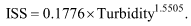
To derive an estimate of A, data from Klamath River samples collected in this reach and stored in the USGS NWIS database were examined for samples in which both TDS, from residue on evaporation at 180 °C, and specific conductance were measured. Most of the 18 samples collected in 1961–62 had calculated values of A from 0.61 to 1.11. No regular spatial or temporal patterns were evident in those data; therefore, the median value 0.69 was chosen as the value for A in equation 1 to derive TDS inputs from hourly or daily specific conductance. Data for 38 groundwater samples collected between 1995 and 2008 near the river (Oregon Department of Environmental Quality, 2009) for which both TDS and specific conductance were measured also resulted in a median value of 0.69 for A, with a range between 0.57 and 0.83. Equation 1 with A = 0.69 was used to generate TDS data from specific conductance measurements at Link River, the Lost River Diversion Channel, the Klamath Straits Drain, and the Klamath Falls WWTP. Only two measurements of specific conductance were available for the effluent of the South Suburban WWTP. Therefore, those measurements were averaged and converted to a constant TDS for that point source. Columbia Forest Products had no existing specific conductance or TDS data; an estimate of 500 mg/L was used in the model. Equation 1 was used in reverse to convert modeled TDS to specific conductance for comparison to measured data during the calibration process. Inorganic Suspended SedimentInorganic suspended sediment (ISS) consists of mineral particles, such as clays, suspended in the water column. This constituent influences water density and light penetration in the model. Direct analyses of ISS were infrequent, but could be correlated to more frequently measured turbidity measurements to estimate ISS concentrations for the model inputs (fig. 4). Turbidity data were collected in triplicate by the Reclamation field crew during trips to maintain the continuous water-quality monitors, resulting in approximately weekly measurements throughout the year. ISS is determined by measuring the difference in the mass on a filter before and after baking it in a muffle furnace to drive off organic matter. This is similar to subtracting measurements of volatile suspended solids (VSS) from measurements of total suspended solids (TSS). Turbidity is an optical property of water that measures scattering and absorption of light due to suspended and dissolved material, including ISS, algae, and particulate and dissolved organic matter (POM and DOM); but, use of the near-infrared wavelength by turbidity instruments, such as those used to collect this dataset, can help exclude the effect of DOM. Summer samples were excluded from the correlation because algae and POM concentrations are highest during this season; samples were included in the regression only when the qualitative visual algal observation was 0. The relation used to develop ISS inputs was:
The highest measured turbidity used to develop this correlation was <30 nephelometric turbidity units (NTU), as VSS and TSS data were not available for higher turbidities. Greater uncertainties are present when using this equation with turbidities higher than 30 NTU; high turbidities were observed in winter in some tributaries (up to several hundred NTU) but these occurrences were infrequent. Summer ISS concentrations for the Link River, Lost River Diversion Channel, and Klamath Straits Drain inflows were set at approximately 5.0 mg/L. Only TSS (not ISS) data existed for the NPDES-regulated point sources. With the assumption that most of those suspended materials would be of organic origin, the ISS for the NPDES point sources was estimated to be 0 mg/L. AlgaeThe CE-QUAL-W2 model allows the simulation of multiple algal groups, limited principally by the availability of supporting data. Data on the amount and species composition of algae in the Klamath River were available for April–November 2007 and 2008 (Sullivan and others, 2008, 2009). Examination of the spatial and temporal patterns in the algal species and biovolume data led to a logical and data-supported separation of the Klamath River algae community into three groups for this model:
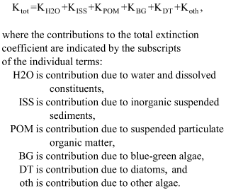
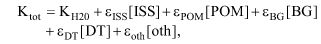
The blue-green algae, also known as cyanobacteria, dominate the assemblage in summer and consist largely of AFA with less frequent occurrence of Anabaena flos aquae. Diatoms are common in the Klamath River upstream of Keno Dam during spring, with species such as Fragilaria capucina var. mesolepta, Stephanodiscus astraea var. minutula, Asterionella formosa, and Melosira granulata. The “other” algae group from the Klamath River data includes species such as Chlamydomonas sp. and Cryptomonas erosa. The algae species data for the Klamath River are reported as cell density (number per milliliter of sample) or biovolume (cubic microns per milliliter) estimates, but the model requires input in units of dry weight concentration (gram per cubic meter or milligrams per liter). Algal carbon was calculated from biovolume by using an equation from Rocha and Duncan (1985). This equation was developed by compiling results from 47 studies of various freshwater algal species that reported both cell volumes and cell carbon concentrations. Once the algal carbon concentration was obtained, the algal carbon to organic matter ratio was applied, of which the derivation is described below. Some required model inputs, including algal and particulate organic matter concentrations, were not directly quantified at inflow sites in winter and during 2006 and 2009. These input concentrations were estimated by using qualitative observations, seasonal concentration patterns from other years, or analysis of trends in data at nearby sites. For example, blue-green algae concentrations were important to include in the models because they are critical to the water quality in the Link–Keno reach. Qualitative algal density observations from Reclamation were used to develop quantitative estimates to fill data gaps. The Reclamation field crew visually inspected the water for the presence of algae during each field site visit, and recorded the visual observation as a number from 0 to 5, ranging from “not visible” (0) to “dense” (5). These observations were made approximately weekly during site visits for grab sampling, sonde deployment, and sonde retrieval. These visual observations would note the presence of large algae such as AFA, but are not generally indicative of less visible algae such as diatoms. Comparisons to measured algal biovolume and species data were made for dates and sites where data were available (fig. 5). Directly measured blue-green algal biovolume and species data were used first for model input; estimates from field observed algal density were then used to fill out input datasets for periods with no other algal data. These estimates were used for 2006 for Link River and Klamath Straits Drain; 2009 for Link River, Lost River Diversion Channel, and Klamath Straits Drain; 2007 for Klamath Straits Drain and Lost River Diversion Channel, and part of 2008 for Lost River Diversion Channel. As a secondary source of algal information when direct sample data did not exist, the seasonal patterns in the algae input datasets were compared to chlorophyll a data measured by the Klamath Tribes at the Pelican Marina site in Upper Klamath Lake in the vicinity of Link Dam (fig. 1). Minor modifications to the seasonal patterns in the estimated Link River datasets for 2006 and 2009 were made after this comparison from the added knowledge about temporal patterns in algae population dynamics for short periods without direct algal data. Organic MatterOrganic matter in CE-QUAL-W2 is separated into four compartments based on relative rates of decay (fast [labile] or slow [refractory]) and its physical status (particulate or dissolved). Dissolved and particulate organic matter (DOM and POM, respectively) are designated as labile (L prefix) or refractory (R prefix). Labile dissolved organic matter, for example, is designated as LDOM. The process of converting laboratory measurements into concentrations of LDOM, RDOM, LPOM, and RPOM for model input required several assumptions and insights based on data and experiments. To determine the concentration of DOM, measured dissolved organic carbon concentrations were converted using the organic carbon to organic matter ratio (derivation described below). In summer, Link River and Lost River Diversion Channel DOM were partitioned into 8 percent LDOM and 92 percent RDOM; Klamath Straits Drain was partitioned into 5 percent LDOM, and 95 percent RDOM. The LDOM for these three inputs was lowered to 1 percent in winter. These partitionings were based on general knowledge that DOM tends to be refractory and specific knowledge from biochemical oxygen demand (BOD) experiments showing DOM to be refractory in the Upper Klamath River (Sullivan and others, 2010). The data also showed a seasonal component for decay rates for this mostly refractory material, with higher lability in summer. Klamath Falls and South Suburban WWTP inflows to the Klamath River were set at 10 and 15 percent LDOM, respectively, throughout the year. The Columbia outfall DOM was partitioned to 95 percent LDOM to approximate the measured BOD values. These point sources were not assigned a seasonal component because the source material was assumed to stay fairly constant through the year. To determine the concentration of POM for Link River, Lost River Diversion Channel, and Klamath Straits Drain, the concentration of live algae was subtracted from the total particulate organic matter concentration, which was derived from measured particulate carbon and the organic carbon to organic matter ratio. In summer, Link River and Lost River Diversion Channel POM was partitioned into 80 percent LPOM and 20 percent RPOM, and Klamath Straits Drain POM was partitioned into 50 percent LPOM and 50 percent RPOM. In winter, the fraction of LPOM for all three of these inputs was lowered to 1 percent. These partitionings are based on BOD experiments that showed summer algal-derived particulate matter in the Link–Keno reach decomposed quickly (Sullivan and others, 2010). Whereas algae, in general, are a source of labile organic matter, blue-green algae are an especially labile form of algae, perhaps because they lack a cellulose wall (Boers and others, 1991). The BOD experiments showed less lability in Klamath Straits Drain, probably due to a larger variety of algal species and organic matter from a different source than Upper Klamath Lake. Fewer data were available to characterize the concentration and lability of organic matter in winter. Because the large algal blooms do not occur in winter, it was assumed that winter particulate organic matter was sourced more from terrestrial plant detritus or decaying macrophytes, older material which is rich in cellulose and lignin and much less labile than blue-green algae. Klamath Falls WWTP and South Suburban WWTP inflows were set at 65 percent LPOM throughout the year; measured BOD was used to estimate the labile-refractory organic matter split for those inflows. The Columbia outfall POM was partitioned to 95 percent LPOM to approximate the measured BOD values. Abundance data for bacteria and zooplankton in this reach of the Klamath River provide useful insights and checks on the ranges of the estimated algal and POM data. Although bacteria and zooplankton are not explicitly represented in this model (they are part of the particulate organic matter fraction), the bacteria and zooplankton measurements were converted to carbon concentration to compare to particulate organic carbon and algal carbon. Bacteria biovolumes were converted to bacterial carbon using a conversion factor from Nagata (1986). Zooplankton densities were converted to zooplankton carbon using equations from the U.S. Environmental Protection Agency (2003) and ratios of body length to dry body weight (Allan Vogel, ZP’s Taxonomic Services, written commun., November 2009); the dry body weights were converted to carbon using a dry weight:wet weight conversion factor and an estimate of zooplankton carbon per unit biovolume (Latja and Salonen, 1978). These calculations show that in summer, depending on the date, either algal biovolume or nonliving POM (dead algae, detritus) made up most of the carbon biomass in the water column at the Link River site, followed by zooplankton and bacteria. The predominance of algae as a proportion of total particulate organic matter biomass in this predominantly eutrophic system is similar to the biomass partitioning observed by Auer and others (2004) in a study of 55 shallow mesotrophic to eutrophic lakes; with increasing eutrophication, phytoplankton, especially blue-green algae, made up a greater proportion of water column particulate biomass compared to bacteria and zooplankton. Distributed Tributary Water QualityFor water temperature, the distributed tributary was estimated to be a mixture of 90 percent surface water and 10 percent groundwater. Groundwater nitrogen, phosphorus, carbon, and oxygen were estimated by examining groundwater data collected by ODEQ from 1995 to 2008 at nonlandfill wells near the upper Klamath River (Oregon Department of Environmental Quality, 2009). Algae and ISS were set to 0 for the groundwater part of the distributed tributary inflow. The surface-water part of the distributed tributary was assumed to have a TDS equal to that from the Klamath Straits Drain. Groundwater TDS concentrations were estimated as a constant 300 mg/L by examining the groundwater specific conductance contour map of the area by Sammel (1980) and from measured TDS values from 1995 to 2008 (or specific conductance converted to TDS) in nearby wells (Oregon Department of Environmental Quality, 2009). Water-Quality ParametersCE-QUAL-W2 requires a large number of model parameters (tables 4and5) that are used in the numerical representation of water-quality processes. These include rate constants, element ratios (stoichiometry), and a wide range of coefficients, half-saturation constants, and other parameters that specify the implementation details of the model algorithms. To construct an accurate and predictive model, parameters should be based on measurements or literature values, if available. The derivation of certain model parameters from data or the literature for the Link–Keno reach of the Klamath River is described in the following sections. Parameters for which there were limited information, or which may vary over a defined range, were adjusted during model calibration. The response of the model to selected parameters, especially those not based on data or literature values, was examined in sensitivity tests to determine their relative importance. Algal and Organic Matter StoichiometryThe model relies on a set of stoichiometric parameters that define the dry mass ratios of carbon, nitrogen, and phosphorus to total organic matter in algae and organic matter. Default model values for AC, AN, AP (the algal ratios for carbon, nitrogen, and phosphorus) and ORGC, ORGN, and ORGP (the organic matter ratios for carbon, nitrogen, and phosphorus) are 0.45, 0.08, and 0.005, respectively, such that the algal ratios are identical to the organic matter ratios. The parameter values used in this model (tables 4 and 5) were based on values from data, which were then adjusted during model calibration. Two datasets were used: (1) particulate organic carbon, particulate organic nitrogen, and particulate organic phosphorus collected at six samplings between mid-July and late September 2008 at Link River and Railroad Bridge by Watercourse Engineering, Inc. (Deas and Vaughn, 2011); and (2) particulate carbon and nitrogen samples collected weekly at a number of sites between April and November of 2007 and 2008 by Reclamation and analyzed by the USGS (Sullivan and others, 2008, 2009). These particulate data were derived from measurements of the composition of material captured from a water sample on a glass fiber filter (0.7 µm pore size), which would include contributions from algae, zooplankton, and particulate organic matter. The latter dataset showed that there was seasonality to the particulate C:N ratio in the Klamath River, with lower values in summer. This seasonality could have resulted from the presence of nitrogen-fixing blue-green algae in summer, which allows atmospheric nitrogen to be an additional source of nitrogen to that algal group. However, the model does not allow seasonal variation for these stoichiometric ratios. These ratios were adjusted during calibration and final values of AC, AN, AP (and ORGC, ORGN, and ORGP) were 0.46, 0.059, and 0.004, respectively. On a molar basis, this provides a 33:1 N:P stoichiometry, which is within the range of values measured by Deas and Vaughn (2011). In addition to the ratios of C, N, and P to organic matter, the CE-QUAL-W2 model requires a value for the mass ratio between algal biomass and chlorophyll a. This ratio is used to convert model output into chlorophyll a concentrations for comparison to measured data. Although constant in the model, this ratio has been reported to be extremely variable, tied to light conditions and nutrient supply (Reynolds, 2006). Ratios of algal biomass to chlorophyll a were calculated using measured chlorophyll a data and algal biomass estimates from the Klamath River at Railroad Bridge, Miller Island, KRS12a, and Keno. Bearing in mind the inherent variability, a median calculated value of 0.031 mg algae per µg chlorophyll a was used in the model. Algal Rates and CoefficientsThe CE-QUAL-W2 model simulates algal growth, respiration, excretion, mortality, and settling, and requires rates and coefficients, as well as half-saturation values for phosphorus- and nitrogen-limited growth and light saturation at the maximum photosynthetic rate. Each of the modeled algal groups requires values for these rates and coefficients as well as some parameters that define the temperature dependence of these processes (table 5). The rates used in the model are guided by values reported in the literature for similar types of algae, though rates can vary depending on a variety of factors; for example, growth rates are dependent on light, nutrient conditions, and water temperature at the time of measurement (Reynolds, 2006). The rate of algal growth in the model is a maximum gross value not adjusted for losses such as respiration, mortality, excretion, or sinking. Algal growth rates in the model are temperature dependent. Temperature parameters were adjusted to define the blue-green and other algae as warm-water algae, and the diatoms as cool-water algae (see parameters AT1–AT4 in table 5). The mortality rate for algae is meant to simulate several processes that are not explicitly included, such as physiological mortality, grazing by zooplankton and other organisms, and death due to pathogens and parasites. This rate is difficult to estimate, especially with scarce data on phytoplankton pathogens and parasites, and is a parameter that is best left for final adjustment during model calibration. Settling of algal cells is included in the CE-QUAL-W2 model and can be positive (sinking) or negative (buoyant) to account for the ability of some algae to control their buoyancy. Settling velocities for algal particles are summarized from the literature in the CE-QUAL-W2 user manual and range from 0.0 to 30.2 m/d (Cole and Wells, 2008). Blue-green algae are unique in that many species, including AFA, are able to regulate their buoyancy with gas vacuoles and by producing and using carbohydrates and other ballast material, resulting in net settling rates that can be positive or negative during specific periods. The model algorithms in CE-QUAL-W2 do not allow the settling rates to vary over time. Algal settling rates for these Klamath River models were largely set through the calibration process. Nutrient-limited algal growth due to lack of nitrogen or phosphorus is simulated in CE-QUAL-W2 according to a Michaelis-Menten model of half saturation. The model half-saturation coefficient for nitrogen-limited algal growth, AHSN, is defined as the inorganic nitrogen concentration (ammonium plus nitrite plus nitrate) at which the light-saturated growth rate is half of its maximum. Because certain blue-green algae, including AFA, can fix nitrogen from dissolved N2 gas (from the atmosphere), their half-saturation coefficient for nitrogen-limited growth was set to 0, indicating that no nitrogen limitation was imposed. Nitrogen isotope δ15N values for AFA collected at Link Dam in July 2008 were near 0 (Deas and others, 2009), which is an indication of N2-fixation from the atmosphere (Vuorio and others, 2006). Calibrated values for diatoms and other algae were within the range of values cited by Cole and Wells (2008) and Padisak (2004). The model half-saturation coefficient for phosphorus-limited algal growth, AHSP, is defined as the phosphorus concentration at which the light-saturated growth rate is half of its maximum. Calibrated values for blue-green algae, diatoms, and other algae were within the range of values presented by Padisak (2004) and Cole and Wells (2008). In addition to limitations on the algal growth rate caused by a lack of nutrients (nitrogen and phosphorus), the amount of available light is a critical factor affecting the algal growth rate. The model requires the user to set light saturation intensity at the maximum photosynthetic rate for each algal group. AFA is a “shade” species that grows well in lower light conditions due to its broader absorption spectrum. For example, AFA has been documented to grow faster than Anabaena under low light conditions (De Nobel and others, 1998). Light Extinction CoefficientsLight extinction coefficients are used by the model to attenuate light through the water column, thus distributing heat vertically in the waterbody and adjusting the light intensity available for photosynthesis with depth. An accurate representation of light extinction is important for modeling both water temperature and algal growth. Light extinction by water and its dissolved constituents, by inorganic suspended solids, by organic suspended solids, and by each group of algae all contribute to the total light extinction coefficient, Ktot:
The model requires separate light extinction coefficients for each contributing factor, thus computing the total light extinction coefficient as a function of the amount of each substance present:
where ε is the extinction coefficient for the component and the value in square brackets [ ] refers to the concentration of the component. To derive the component light extinction coefficients (ε) for model input, the total light extinction coefficient Ktot was first determined for the existing data during April–November of 2007 and 2008 at the Railroad Bridge, Miller Island, KRS12a, and Keno sites. Ktot can be determined from light intensity measurements collected as a function of depth and an application of the Beer–Lambert law of light absorption. Alternatively, Secchi depth measurements, made by lowering a Secchi disk into the water and recording the maximum depth at which its pattern is still visible from the surface, can be used to estimate the total light extinction coefficient using equations such as those by Poole and Atkins (1929), Idso and Gilbert, (1974) or by Williams and others (1980). The light meter and Secchi disk methods were compared for the Link–Keno reach using a dataset from Deas and Vaughn (2006). The resulting light extinction coefficients calculated from light meter data were similar to light extinction coefficients derived from Secchi disk data and a modified Poole and Atkins equation (fig. 6). Secchi disk data collected by the Reclamation field crew during each water-sample collection trip were used with the Poole and Atkins equation to estimate total light extinction coefficients at Klamath River nonboundary sites. After computing the total light extinction coefficient values, the results were correlated with the component concentrations (ISS, POM, and algae measured or estimated as described in the previous discussion) using multiple linear-regression methods to derive estimates of the component light extinction coefficients (ε) and KH2O, the baseline light extinction due to water and dissolved substances (the regression intercept). The multiple linear-regression analysis was performed using the R statistical software (http://www.r-project.org/) to extract the extinction coefficients for each component (tables 4 and 5, values for EXH2O, EXSS, EXOM, and EXA). The derived extinction coefficient for water was 1.217/m, a relatively large value that is indicative of, and consistent with, a substantial concentration of dissolved organic matter that imparts a color to the upper Klamath River. The value of BETA, which describes how much solar radiation is absorbed at the water surface, was set to the default value of 0.45. Organic Matter Decay and Settling RatesDecay and settling rates for particulate organic matter are required model inputs for CE-QUAL-W2 that are critically important for the Link–Keno reach of the Klamath River. Organic matter decay rates were estimated from the results of BOD experiments (Sullivan and others, 2010) that included both unfiltered and coarse-filtered samples. The Klamath River BOD samples had both labile and refractory components that were closely related to the concentrations of particulate and dissolved organic matter in those samples. Model values for several organic matter decay rates in the model (LDOMDK, LPOMDK in table 4) were derived from these experiments, with refinement during model calibration. Experiments indicated that refractory decay was slow; the values used in the model also were adjusted during calibration. Studies were conducted in the Klamath River in 2008 to provide reach-specific settling rate data for the model (Deas and Vaughn, 2011). A Laser In-Situ Scattering and Transmissometry with Settling Tube (LISST-ST) instrument (Sequoia) was deployed in the Link–Keno reach at the Railroad Bridge sampling site. In-situ settling rates were assessed from three 1-week experiments that were performed during August and September 2008. Depending on the sampling date and particle size, settling rates ranged from less than 0.2 to greater than 100 m/d for particle sizes ranging from less than 5 to greater than 350 μm. These settling rates represented all particulate matter in the water column, including dead organic matter, living algae, and zooplankton. Larger particles (>350 μm) formed a large fraction of the particulate matter entering the Klamath River from Link River. These particles tended to have high settling rates, ranging from less than a meter per day to tens of meters per day or higher. An examination of the data from all experiments identified a median settling rate of 2.5 m/d. Smaller size fractions were examined (<62 μm, where 62 μm is the breakpoint between silt and sand) (American Society of Civil Engineers, 2000), to provide further insights into estimating settling rates for consideration in the model. The median measured settling rate was 0.44 m/d for particle sizes less than 62 μm. Additional information gleaned during LISST-ST deployment and from more recent, detailed modeling focusing on the Lake Ewauna part of the Link–Keno reach indicates that other factors important to settling rate estimation may be occurring near or at the Railroad Bridge site. First, Link River introduces a disproportionate fraction of large particulate matter (> 350 μm), which is consistent with field data (Sullivan and others, 2008 and 2009). Second, the Lake Ewauna reach has complex hydrodynamics, including the formation of gyres, potentially influencing particle size distribution and settling rates. Finally, higher river flows affect turbulence, can resuspend some particulate matter, and thereby affect measured settling rates of particles. Reclamation conducted a surface-water spill study from July 28 through October 3, 2008, to examine methods to reduce entrainment of certain fish species (Marine and Lappe, 2009). Sub-daily flow ranges during this period ranged from less than 500 to about 3,000 ft3/s, but typically ranged from 500 to 1,500 or 2,000 ft3/s. Aside from the spill study, flows generally were stable throughout the day. This proximity of the Railroad Bridge site to Link River can result in larger particles being present at this location than in downstream reaches of the river. This condition can be exacerbated by local hydrodynamics of Lake Ewauna proper. Furthermore, the dynamic, high-flow conditions imposed by Reclamation during the 2008 flow experiment could have reduced travel time through Lake Ewauna and re-entrained settled material from the bed. Because CE-QUAL-W2 does not accommodate variable settling rates (temporally or spatially), an average or representative settling rate was considered for the entire Link–Keno reach. The ultimate settling rate for particulate organic matter applied at the reach scale was 0.25 m/d, although actual settling rates may be higher in the upstream part of the system. Phosphorus and NitrogenThe CE-QUAL-W2 model includes several algorithms to mimic denitrification and the oxic or anoxic releases of nutrients in an attempt to simulate nutrient fluxes at the sediment–water interface. In one such process, the release of phosphorus from sediments under anoxic conditions (PO4R, table 4) is specified as a fraction of the model’s zero-order SOD rate. Conversely, nutrients can be released to the water column under oxic conditions by the decay of organic matter in the sediments compartment, which creates the model’s first-order SOD. Loss of nitrate and inorganic nitrogen through denitrification can occur where oxygen conditions are depleted and specialized bacteria use nitrate (rather than oxygen) as a terminal electron acceptor. The model also can approximate denitrification through an optional mechanism that allows nitrate to diffuse into the sediments where it is converted or utilized. The release rate of ammonia from sediments under anoxic conditions (NH4R, table 4) is specified in the model as a fraction of the zero-order SOD rate. The oxidation rate of ammonia (nitrification) also is a specified model parameter. Sediment Oxygen DemandRates of consumption of dissolved oxygen at the sediment–water interface (SOD) have been measured in the Link–Keno reach of the Klamath River by several groups of researchers. In-situ SOD studies were conducted in this reach in early June 2003, prior to the influx of the blue-green algae from Upper Klamath Lake (Doyle and Lynch, 2005); the median measured SOD rate was 1.8 (g O2/m2)/d at 20°C. Laboratory-based SOD studies (Raymond and Eilers, 2004; Eilers and Raymond, 2005) using sediment cores gave similar values. The CE-QUAL-W2 model has two mechanisms to simulate SOD: zero-order and first-order. The zero-order process allows the sediment to exert a relatively constant oxygen demand, with the rate modified only by water temperature. First-order SOD, however, keeps track of all organic matter and algae that settle to the sediment. More organic matter in the sediment compartment means more oxygen demand, which is important for simulating the response of a large flux of settling algae in the Klamath River in midsummer. The CE-QUAL-W2 model calculates a decay rate for the first-order sediment compartment based on the individual decay rates of algae, LPOM, and RPOM, and weighted by the amount of each that has settled to the river bottom. Both SOD mechanisms, but especially the first-order demand, were used in these models to produce a dynamic representation of the seasonal variation in SOD. The SOD temperature factors also were adjusted during model calibration. ReaerationThe model user must select one of many possible equations in CE-QUAL-W2 to represent the reaeration of oxygen across the air–water interface. Rivers are usually assigned reaeration equations based on river depth and water velocity. Lakes are usually assigned reaeration equations based on depth and wind speed. A number of reaeration equation options were tested; the lake equation 14 was used in the final model, due to the low velocities and strong effect of wind in this reach:
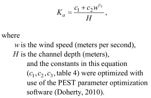
|
First posted July 14, 2011 For additional information contact: Part or all of this report is presented in Portable Document Format (PDF); the latest version of Adobe Reader or similar software is required to view it. Download the latest version of Adobe Reader, free of charge. |

![]() U.S. Department of the Interior |
U.S. Geological Survey
U.S. Department of the Interior |
U.S. Geological Survey
URL: http://pubsdata.usgs.gov/pubs/sir/2011/5105/section3.html
Page Contact Information: GS Pubs Web Contact
Page Last Modified: Thursday, 10-Jan-2013 20:07:22 EST

 (1)
(1)
 (2)
(2)
 (3)
(3)
 (4)
(4)
 (5)
(5)