Four-Band Image Mosaic of the Colorado River Corridor Downstream of Glen Canyon Dam in Arizona, Derived from the May 2013 Airborne Image Acquisition

Image Processing

The data delivered by Fugro Earthdata Inc. were checked for smear, shadow extent, and water clarity, as described for previous image acquisitions by Davis (2012). We then produced a corridor-wide mosaic, using the best possible tiles with the least amount of smear, the smallest shadow extent, and the clearest, most glint-free water possible. During the mosaicking, some adjacent tiles needed to be spectrally adjusted to account for differences in date, time, Sun angle, weather, and environment. We used the same method as that of Davis (2012) for the spectral adjustment, and we kept adjustments within 10 percent of the original data values to maintain integrity as closely as possible. Adjustments were applied to all bands of any single tile equally. During the mosaicking, we determined that the individual Leica ADS80/82 sensors on the two different aircraft did not have perfect intersensor calibration in the red band. To adjust for the miscalibration, all values in the red bands from the objectionable sensor were multiplied by 1.1133. In contrast to previous data acquisitions (Davis, 2012), severe monsoonal rainstorms were not an issue in 2013, and so the data-acquisition period was relatively short and the variation in river sediment (water color and clarity) relatively low.

To address the issue of spectral comparison between collection years, we needed to determine that the spectra from the 2009 image dataset and the 2013 images were analogous. First, we needed to identify the correct stable ratio for the spectral bands. For this purpose, we identified perfectly registered pixels in areas of surface materials that were least likely to change during the 4-year intercollection period between 2009 (Davis, 2012) and 2013. For these select pixels, we determined the following band ratios for the 2009 and 2013 data, separately: green/red and red/NIR. We assumed that the spectral ratios calculated with the 2009 pixels were correct and then applied calculations to adjust the 2013 pixel ratios to match those calculated for 2009. We worked first with the red band because of concern that making all the spectral adjustments in the NIR would potentially saturate this band. We then determined a mean adjustment factor for application to the 2013 red band that made the 2013 green/red ratio equal to that for the 2009 data. The adjustment factor that we applied to the 2013 red band is given by:

where R_i is the initial state of the red value as delivered by Fugro Earthdata Inc. and R_f is the final value postadjustment. We next determined an adjustment factor to apply to the 2013 NIR band that made the 2013 red/NIR ratio equal to that for the 2009 data. The adjustment factor that we applied to the 2013 NIR band is given by:

where NIR_i is the initial state of the NIR value as delivered by Fugro Earthdata Inc. and NIR_f is the final value postadjustment.

The final adjusted mosaic was then subset to the GCMRC quarter-quarter-quadrangle (QQQ) system (fig. 3), with 10 to 15 m of overlap between images. The QQQs were then registered to the 2009 four-band imagery because a primary reason for acquiring the data was to detect change relative to previously acquired image datasets.

To demonstrate the corridor-wide digital-number (DN) variation in the final mosaic of images, we calculated the 1st and 99th percentile of derived 12-bit digital numbers for each wavelength-band image in all the image tiles (fig. 4). The 1st percentile is relatively stable between images (that is, throughout the river corridor; fig. 4); minor fluctuations were attributed to daily variations in atmospheric water-vapor content from changing weather and to the amount of topographic shadowing within each image tile, in which reflectance is dominated by atmospheric scattering. The 99th percentile varies much more widely, owing to similar but accentuated factors governing the 1st percentile, with the additional effect of average scene geology, sand content, and vegetation.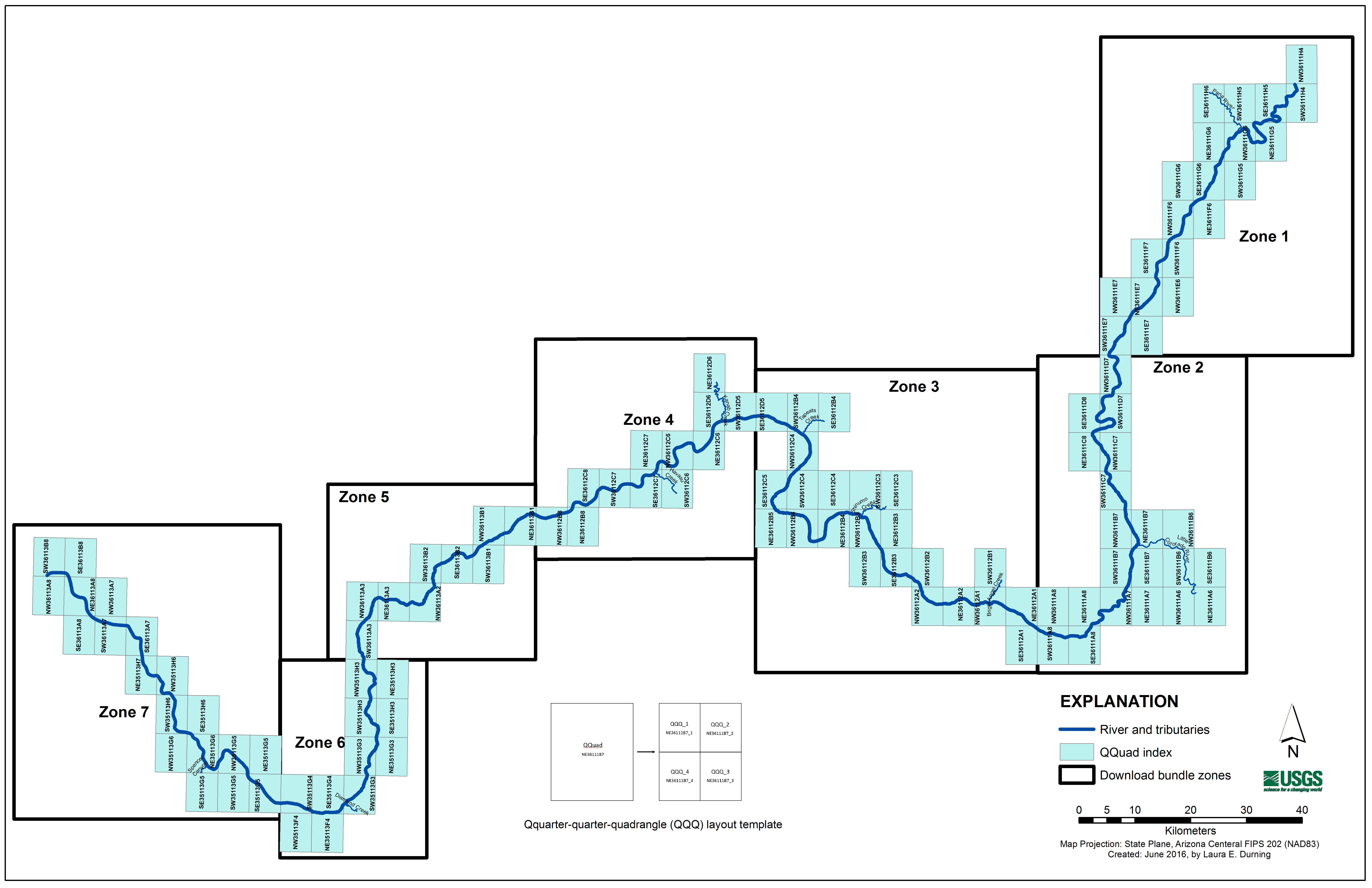

Figure 3. U.S. Geological Survey (USGS) Grand Canyon Monitoring and Research Center index map showing USGS quarter-quadrangles (QQ). Many image files adhere to quarter-quarter-quadrangle (QQQ) system, so please refer to the layout template. Each of seven zones shown here can be accessed as a compressed zip file.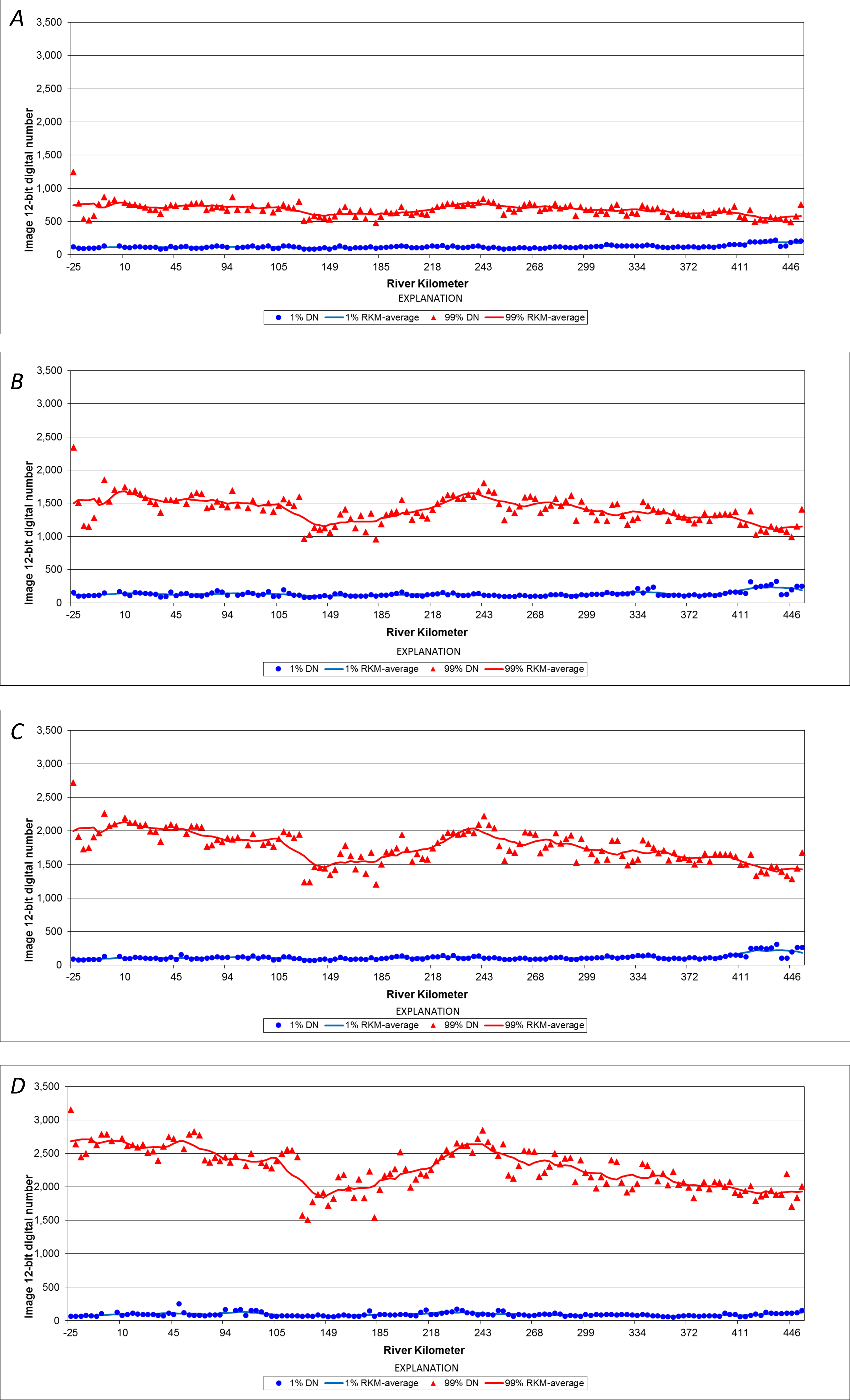

Figure 4. Graphs showing 99th percentile (red triangles) and 1st percentile (blue circles) digital numbers (DN) relative to river kilometer in each of the four spectral bands: A, Blue band (0.430–0.490 µm); B, Green band (0.535–0.585 µm); C, Red band (0.610–0.660 µm), and D, Near infrared (0.835–0.885 µm). Moving averages (lines) were determined from the neighboring four-image scenes centered on river-kilometer increments.