U.S. Geological Survey Data Series 671
Side scan sonar is used to detect seabed features, material, and textures from acoustic backscatter response intensity. In this application the instrument (towfish) is towed by a cable aft of the vessel. Once activated, a fan-shaped acoustic pulse is repeatedly emitted downward to the seafloor, perpendicular to a vessel's navigation track, collecting a series of swaths stitched together to create a sonogram, or seafloor image. The towfish can be operated with a range of frequencies; lower frequencies are recorded at a lower resolution but increasing swath range, and higher frequencies are recorded with high resolution at the cost of swath range. High-intensity returns are indications of hard or dense surface material, such as rock or hard-packed sand, whereas low-intensity returns may infer silt or organic material. Intensity images are used in conjunction with physical "grab" samples or cores for the purpose of ground truthing the side scan mosaic.
Side Scan Sonar Acquisition System Components
The side scan sonar components used during Cruise 10CCT03 are as follows:
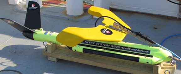
Figure 6. Photograph of the Klein 3900 side scan sonar system used for data collection. |
During the 10CCT03 cruise a Klein 3900 dual-frequency side scan sonar system (fig. 6) was towed on the starboard side of the vessel to collect information about surface sediment material. SSS was acquired and recorded using SonarPro software in an Extended Triton Format (XTF). Differential GPS position was obtained from two NGS CORS beacons (Mobile and English Turn), recorded by the Trimble DSM 212 system and output in the World Geodetic System of 1984 (WGS84). The towfish altitude varied considerably during the cruise due to the nature of shallow-water surveying operations. Ideally, SSS is flown at a relatively considerable distance from the vessel and other instruments to avoid acoustical interference. Typical sources of acoustical interference are vessel vibrations and other acoustical instruments that utilize similar frequency ranges. However, in shallow-water surveying the optimal distance is difficult to achieve due to the negative buoyancy of the towfish and the effect of unanticipated isolated shoals.
Side Scan Sonar Processing
Data files collected in XTF format were converted into CARIS data format structure called Sonar Information Processing System (SIPS) for the purpose of editing and side scan mosaic creation. All horizontal positions were offset relative to the position of the Applanix POS MV antenna.
The first step in SSS data processing was to correct the altitude, or first return. This was achieved by a combination of auto-prediction parameters and manual boundary digitization of the water column and seafloor.
The second step was application of the beam pattern correction, which was accomplished by sampling a series of beams over homogeneous surface content. The purpose of beam pattern correction is to identify and offset the inherent instrument intensity variance as the across-track range increases. Near nadir the acoustic return is significantly more intense and decreases as across-track range increases. These phenomena result in a false high-intensity value strip along the center line of the SSS swath.
Several other SSS editing tools were applied, including angle-varying gain (AVG) and time-varying gain (TVG) corrections, which were used to further smooth the resulting intensity range artifacts, offering a more consistent along- and across-track image. The despeckle editing tool was also employed to identify and mute isolated pixels having extreme high- or low-intensity values relative to adjacent pixels.
After all the individual side scan line files were examined and edited, Geo-referenced Backscatter Rasters (GeoBars) were created. For this dataset, a resolution of 1 m was chosen. From the series of GeoBars, a side scan mosaic image was generated as a composite of the GeoBars, which also provides for a continuous image of a single intensity value range for geographic comparison.
In shallow-water surveying (depth 15 m or less for this cruise), a variety of technical phenomena such as multipathing and ping ghosting proved problematic for processing SSS data. Multipathing is the bouncing of the signal off the ocean surface and seabed before return. This phenomenon is amplified by wave chop, rough weather, and shallow depths. Ghosting is another acoustic anomaly produced by a ping rate which is not slow enough for the transducers to decipher one ping from another. This echoing effect is especially the case in very shallow depths (Hayes and Barclay, 2003).
The overall side scan mosaic (fig. 12) can be viewed on the Images page. Figures 13 and 14 are close up side scan mosaic views of the east and west sections respectively. Also, the GeoTIFF image can be found in the Data Products folder. Please reference the read-me file for file names and details.
A multibeam system emits a sound pulse from a single transducer head. Multiple sensors within the transducer head are set at different angles to listen for the sound pulse return, ultimately resulting in an array of depth measurements. The directional orientation of the transmit beams is parallel to the trackline, and the directional orientation of the receive beams is perpendicular to the trackline (fig. 7). A multibeam system detects the seafloor by measuring the peak amplitude of the incoming echo return. The peak amplitude method uses the travel time of the beam to calculate the slant range of the beam, producing a depth value where that beam interacted with the seafloor or other object (for example seawall, pier). This depth measurement is then further corrected for boat motion (heave, roll, and pitch), differential GPS positioning, and sound velocity (SEA Ltd., 2005, HYPACK Inc., 2009).
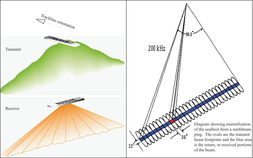
Figure 7. Diagram showing the transmit and receive orientation of a multibeam system's beams and the ensonification of the seafloor from one cycle, also known as a ping. Diagram modified from HYPACK (2009). |
Multibeam System Acquisition Components
The mulitbeam system components used during Cruise 10CCT03 are as follows:
The multibeam bathymetry was collected using the RESON SeaBat 8125 System. This system uses a frequency of 455 kHz with a maximum swath angle of 120 degrees (fig. 8 and fig. 9). The Applanix POS MV provided boat motion from the Internal Motion Unit (IMU), and heading from two Novatel 531 Choke Ring antennas. GPS for navigation was acquired using the Trimble DSM 212 antenna with a beacon receiver. The Trimble antenna (fig. 10) received the broadcasted correction from the NGS CORS reference beacons (Mobile and English Turn), which provided the differential navigation at 1 pps for multibeam operations.
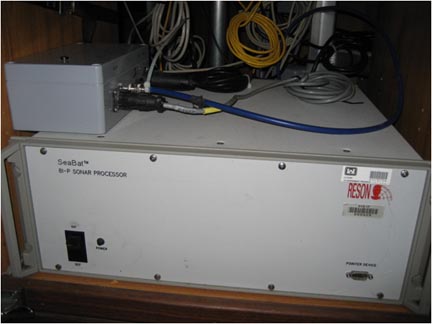
Figure 8. Photograph of the RESON SeaBat 8I-P sonar processor with the sounding head velocity probe box mounted on the top left. |
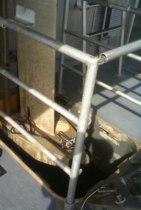
Figure 9. Photograph of the RESON SeaBat 8125 mounted on a retractable strut-arm that is lowered between the catamaran hulls of the the SV Irvington. The sound velocity probe is positioned aft of the strut arm. |
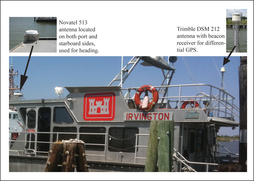
Figure 10. Photograph of the SV Irvington showing location of the Novatel 513 antennas used with the Applanix POS MV and the location of the Trimble DSM 212 antenna and beacon used for differential navigation. |
Multibeam System Field Calibration and Acquisition
HYPACK, Inc., HYSWEEP version 10 was used for the multibeam data acquisition, system calibration, and data post-processing. A patch test was performed at the beginning of the survey to calibrate the SEABAT 8125 and included latency, roll, pitch, and yaw. This involved collecting multibeam data along lines over a sloping surface for the latency, pitch, and yaw tests and over a flat surface for the roll test. All multibeam lines were collected in HYSWEEP raw data format (HSX). The HSX lines were imported into the patch test module of HYSWEEP's Mulitbeam Max editor (MBMAX) and converted into HYSWEEP edited binary file formats (HS2). The resulting offsets from the patch test were applied to the hardware configuration file prior to survey data acquisition. The Applanix POS MV is not a gyro but uses inertial GPS technology and therefore did not need calibration.
During data acquisition, the differentially corrected positions supplied through the Trimble DSM 212 interface were recorded in the WGS84 datum. Ship heading and motion (roll, pitch, heave) were measured by the Applanix POS MV motion unit. Sound velocity was recorded at the multibeam sonar head. Additional sound velocity casts were conducted at the start and finish of each survey day and as needed throughout the survey. All respective data strings were captured and streamed in real time via HYSWEEP onto a Dell Precision 690 shipboard computer.
Multibeam Bathymetry Processing
Multibeam data post-processing was completed at the USACE in Mobile, Ala., using HYPACK Inc., HYSWEEP version 10. The raw HSX data files were imported into MBMAX editor for post processing. Data for tide correction was obtained from automated tide gages maintained by the USACE and applied at this point within MBMAX. The sound velocity cast data were also applied in MBMAX at this point. The processed x,y,z data files were exported in ASCII format and referenced to WGS84 for the horizontal datum and MLLW for the vertical datum. The x,y,z grid point data for 8 survey days had spacing that ranged from 3 m to 6 m and resulted in 749,867 points ranging from -15.45 m to -2.42 m in depth. This dataset was then transferred to the St. Petersburg Science Center for gridding and incorporation into a larger bathymetric dataset for the GUIS.
The x,y,z ASCII files were imported into ESRI’s ArcMap version 9.3.1, merged together, and gridded using the Geostatistical Analyst tool radial basis function. This tool allowed adjustment to the interpolation parameters with regard to real-data spatial resolution and orientation. The interpolation parameters once set are then used by the tool for predicting values. This method provided a more accurate and less biased representation of the dataset as a whole. A cross-validation report can be generated when using the radial basis function. This helps the user understand how well the model will predict data values at unknown locations. In general the cross validation takes one point and predicts that point's position using the surrounding data values. The result is a predicted value. This predicted value is compared against the actual value of that data point and general statistics computed. Table 1 lists the initial cross validation results of depth values from the multibeam bathymetry for Cruise 10CCT03.
| 10CCT03 Overview | Measured |
Predicted |
Error |
|---|---|---|---|
Points |
749,865 |
749,865 |
749,865 |
Minimum |
-15.45 |
-15.41 |
-5.52 |
Maximum |
-2.42 |
-2.23 |
+4.88 |
Mean |
-9.45 |
-9.45 |
0.00 |
Standard Deviation |
+2.23 |
+2.23 |
+0.119 |
Table 1. ESRI's cross-validation report of depth values from the multibeam bathymetry 50-meter grid for Cruise 10CCT03. |
The trackline layout and broad survey coverage area of Cruise 10CCT03 did not allow for gridding the data in one block. This is reflected in the 9-m error range (maximum +4.88 m to minimum -5.52 m) of the cross- validation report (table 1). The trackline gap that spans the Petit Bois Pass was wider than 7 km, making it difficult to accurately infer bathymetry (fig. 11). To accommodate this, the dataset was split into an eastern and a western section. This improved the gridding results for the eastern section; however, there were still visible problems in the grid of the western section. The problem area was located south of the bend in Horn Island, where the trackline configuration changes from uniform shore-parallel lines to small condensed non-uniform lines. To resolve this, the western section was divided at this location into West Section 1 and West Section 2 (fig. 11).
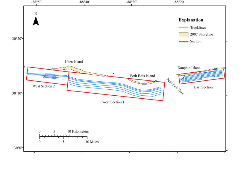
Figure 11. Ship trackline navigation map indicating the three divisions (East Section, West Section 1, and West Section 2) created to enhance the creation of the 50-meter bathymetry grids. |
The division improved the resultant grids; however high error values (+/- 0.60 m) were still reported in the cross-validation report statistics. These high error values were selected and evaluated based upon their location to the surrounding data, and the possible influence on the resultant grid. These data points were either kept or removed. In most cases, the higher error values were associated with the outer edges of the tracklines or along one individual trackline suggesting an isolated problem. Having an isolated problem on one trackline or having problem data at the outer edges of multibeam tracklines is not uncommon. In these cases (for instance) the values were deleted. The radial basis gridding method and review of the cross-validation report was repeated. This iterative method was successful at decreasing the range of error to below +/- 0.50 m for all three sections as identified by the minimum and maximum values in the error columns for each section. Figure 15 is the 50-m multibeam bathymetry grid overview image. The following tables and figures list the final cross-validation results for the East Section (table 2, fig. 16), West Section 1 (table 3, fig. 17), and the West Section 2 (table 4, fig. 18). Once all the grids were completed individually they were merged into one 50-m resolution multibeam bathymetry grid for the survey region.
East Section |
Measured |
Predicted |
Error |
|---|---|---|---|
Points |
333,284 |
333,284 |
333,284 |
Minimum |
-11.18 |
-11.14 |
-0.27 |
Maximum |
-2.42 |
-2.43 |
+0.27 |
Mean |
-8.26 |
-8.27 |
0.00 |
Standard Deviation |
+1.78 |
+1.78 |
+0.03 |
Table 2. Final cross-validation results of depth values from the multibeam bathymetry 50-meter grid for the East Section. |
West Section 1 |
Measured |
Predicted |
Error |
|---|---|---|---|
Points |
255,565 |
255,565 |
255,565 |
Minimum |
-15.45 |
-15.41 |
-0.46 |
Maximum |
-3.44 |
-3.50 |
+0.38 |
Mean |
-11.62 |
-11.62 |
0.00 |
Standard Deviation |
+1.27 |
+1.27 |
+0.05 |
Table 3. Final cross-validation results of depth values from the multibeam bathymetry 50-meter grid for West Section 1. |
West Section 2 |
Measured |
Predicted |
Error |
|---|---|---|---|
Points |
155,370 |
155,370
|
155,370
|
Minimum |
-10.35 |
-10.35 |
-0.38 |
Maximum |
-3.09 |
-3.13 |
+0.38 |
Mean |
-8.37 |
-8.37 |
0.00 |
Standard Deviation |
+1.59 |
+1.59 |
+0.02 |
Table 4. Final cross-validation results of depth values from the multibeam bathymetry 50-meter grid for West Section 2. |
Also, the files can be found in the Data Products folder. Please reference the read-me file for file names and details.

![]() U.S. Department of the Interior |
U.S. Geological Survey
U.S. Department of the Interior |
U.S. Geological Survey
URL: http://pubsdata.usgs.gov/pubs/ds/671/html/equipment_processing.html
Page Contact Information: GS Pubs Web Contact
Page Last Modified: Monday, 28-Nov-2016 18:39:20 EST