Holocene Evolution, OFR 01-076
Home | Intro | Geology | Methods | Animation | Data | GIS | Acknowledgements | References | Appendix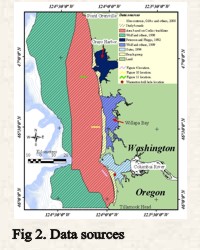 Seismic surveys conducted in 1997 and 1998 by
the USGS (Cross and others, 1998; 1999) covered a large portion of the inner and
middle continental shelf of the CRLC (Fig.
2). To better understand the framework of the CRLC, additional data from the outer shelf,
new data from the barriers, as well as a more complete data from the estuaries (Grays Harbor, Willapa Bay
and Columbia River) needs to be incorporated. Essentially, the methods described in this
section can be broken down into 3 areas: 1) interpretation and
validation of the USGS data, 2) integration of other data sets to form one
uniform data set, and 3) using these results to analyze and visualize the Holocene
evolution of the study area.
Seismic surveys conducted in 1997 and 1998 by
the USGS (Cross and others, 1998; 1999) covered a large portion of the inner and
middle continental shelf of the CRLC (Fig.
2). To better understand the framework of the CRLC, additional data from the outer shelf,
new data from the barriers, as well as a more complete data from the estuaries (Grays Harbor, Willapa Bay
and Columbia River) needs to be incorporated. Essentially, the methods described in this
section can be broken down into 3 areas: 1) interpretation and
validation of the USGS data, 2) integration of other data sets to form one
uniform data set, and 3) using these results to analyze and visualize the Holocene
evolution of the study area.
Cross and others (1998; 1999) give overviews of the data collection techniques during the 1997 and 1998 field seasons. For coherency, a brief description follows. In 1997, seismic-reflection data acquisition used a boomer sound source with a Benthos (URL: http://www.benthos.com) or an ITI hydrophone array. These data were digitally logged to an EPC(URL: http://www.epclabs.com)Labs ADS-640 logging system in EPC 8-bit format. These data were then converted to a standard 16-bit unsigned integer SEG-Y format using a conversion tool supplied by EPC Labs. In 1998, a sparker system was used as the sound source with a Benthos hydrophone array. These data were recorded digitally to a Triton-Elics Delph (URL: http://www.tritonelics.com) acquisition system in a compressed Elics format. Using a Triton-Elics Delph conversion tool, these data were converted to a standard 16-bit signed integer SEG-Y format.
Both data sets underwent minor filtering and enhancement in Landmark Graphics Corporation´s ProMAX (URL: http://www.lgc.com) software prior to being loaded into Landmark Graphics Corporation´s Seisworks (URL: http://www.lgc.com ) seismic interpretation software. For display purposes, these data were converted to an 8-bit signed format for loading into Seisworks. The normalization value used for each line was decided upon by visual inspection combined with histogram information of data values.
The 1997 data set had several additional processing steps that were needed. Depending on water depth and the fact that ¼ second of data were recorded, it was sometimes necessary to put a time delay into the recording. Unfortunately, this delay was not written into the SEG-Y header of the data file. In order to alleviate this problem, the bathymetry data collected concurrently on the cruise were used to shift the seismic profiles in Seisworks. This bathymetry data underwent tide corrections and smoothing post-cruise. This corrected bathymetry was then used as the baseline to shift the seismic reflection profiles by matching the digitized seafloor from these profiles to the corrected bathymetry.
The 1998 seismic data were resampled during the conversion to 8-bit data so that the 1997 and 1998 data sets would have the same sample interval within Seisworks. This resampling simplified data comparison and display in Seisworks without compromising the data itself. Once in Seisworks, the 1998 seismic-reflection profiles were shifted to accommodate tide corrections and bathymetry smoothing in the same manner as the 1997 data.
Loading the data into Seisworks was valuable for several reasons. A variety of enhancements can be temporarily applied to the seismic data greatly aiding the interpretation process. Most significantly, once the interpretation is completed, each horizon can be exported into an X,Y,Z ascii file which is appropriate for importing into other software packages. For this particular data set, the horizons were all exported into a single ascii file of X, Y, Z1, Z2, Z3 with X and Y being the position in meters, UTM zone 10, NAD83. Z1 is depth of the seafloor in milliseconds (ms); Z2 is the depth of the ravinement surface in milliseconds. Z3 is the depth of the lowstand surface in milliseconds. Exporting the horizons to a single file in two-way travel times simplifies future adjustments for the speed of sound corrections. For this study, the speed of sound used in water was 1,500 m/s while the speed of sound used in the sediment was chosen to be 1,600 m/s for the reasons described in the Geologic Discussion section of the paper.
 The digitized interpretation needed to be
gridded to generate maps and make volume calculations possible. However,
gridding was complicated by the uneven data distribution. The survey line
spacing was ~5 km with a very high density of data points along the tracklines
(1/2 second fire rate generates a shot point every ~1.75 m). The gridding of
these unevenly distributed data points was completed with the Dynamic Graphics,
Inc. EarthVision (URL: http://www.dgi.com) software. To capture the detail in the along track direction a small
grid size was warranted while a large cell size would be appropriate for the
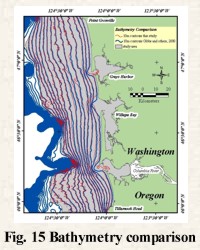
across-track direction. In order to derive the optimum cell size given the
density of data points, the present day sea floor gridded from the seismic data
was compared to the gridding of the more closely spaced NOS bathymetry points by
Gibbs and others (2000) (Fig. 15). The close
agreement of these two data sets indicates the use of a 200 m cell size was justified and therefore the same gridding
parameters were applied to the lowstand and ravinement surfaces.
The digitized interpretation needed to be
gridded to generate maps and make volume calculations possible. However,
gridding was complicated by the uneven data distribution. The survey line
spacing was ~5 km with a very high density of data points along the tracklines
(1/2 second fire rate generates a shot point every ~1.75 m). The gridding of
these unevenly distributed data points was completed with the Dynamic Graphics,
Inc. EarthVision (URL: http://www.dgi.com) software. To capture the detail in the along track direction a small
grid size was warranted while a large cell size would be appropriate for the
across-track direction. In order to derive the optimum cell size given the
density of data points, the present day sea floor gridded from the seismic data
was compared to the gridding of the more closely spaced NOS bathymetry points by
Gibbs and others (2000) (Fig. 15). The close
agreement of these two data sets indicates the use of a 200 m cell size was justified and therefore the same gridding
parameters were applied to the lowstand and ravinement surfaces.
After the above steps, the more difficult task of incorporating data from other sources could begin (Fig. 2). For the modern day surface, this meant incorporating NOS bathymetry points on the outer shelf as well as in the bays and estuaries (NOAA-NGDC, 1998). For the on land portions of the study area, a modified version of the DEM (Digital Elevation Model) as compiled by the Washington Department of Ecology was used (R. Daniels, personal communication). One concern in combining the DEM with the seafloor bathymetry data was the issue of vertical datum. The seafloor bathymetry points are in reference to MLLW (mean lower low water) while the DEM used the vertical datum NAVD88. Fortunately, in the study area, the two vertical datums are offset at most by approximately 0.5 m. Since this offset falls within the resolution of the seismic systems used, and within the accuracy of the fathometer data, no vertical datum adjustment was needed.
An even bigger challenge than the modern day surface was the incorporation of previously published seismic interpretations with the lowstand and ravinement surfaces. The problem was two-fold: 1) How to best merge these data with our data?, and 2) How to make any necessary speed of sound adjustments? In the estuaries (Grays Harbor, Willapa Bay and Columbia River) the ravinement surface is absent, but is equivalent to the flooding surface. The flooding surface in these estuaries is the present day seafloor. The source for these data were primarily NOS bathymetry points as acquired form Michael Hamer (personal communication) as well as a few seismic lines run during the 1997 and 1998 surveys. Offshore, outside the 1997 and 1998 survey area, interpretations by Wolf and others (1997) needed to be incorporated. Initially, the only source of data was the Open-File Report 97-677 paper maps, but communication with Michael Hamer resulted in the acquisition of the Arc/Info (URL: http://www.esri.com) digital files of the interpretations. This saved the time consuming process of digitizing and registering the paper maps. The late Quaternary isopach map from the report by Wolf and others (1997) was compared with our Holocene thickness maps. Where the two data sets overlapped the interpretations were in agreement. A simple way to combine the data from Wolf and others (1997) with our data would have been to use the isopach map added to the already generated seafloor surface. However, the density of the isolines was not sufficient for a satisfactory representation of the ravinement surface. For this reason, it was necessary to combine the structural map of Wolf and others (1997) with our data. Using Arc/Info, each contour line of Wolf´s and others´ (1997) erosional surface was densified to generate a vertex every 100 m. The X,Y, and Z value of each point (Z value referenced to the contour value) was extracted using the Arc Macro Language (AML) script found on the ESRI website (URL: http://www.esri.com) "a2z.aml". These scattered data points were combined with the scattered data points from the inner and middle shelf and regridded in EarthVision. To test the validity of this data incorporation, the ravinement to seafloor isopach map was regenerated and compared the offshore portion of this map to the isopach map of the same area in Wolf and others (1997) ). At this point several problems were encountered. The most obvious problem was the presence of 5-10 m of sediment north of Grays Harbor where no such sediment cover exists on the Wolf´s and others´ (1997) map. In addition, estimated sediment volumes calculated using the polygon areas of Wolf and others´ isopach map didn´t agree with the volumes calculated for the same area using the newly created isopach values. In order to match volume estimates from their interpretation, the area of each polygon of the isopach map was computed within Arc/Info. This information was then placed into a Microsoft (URL: http://www.microsoft.com) Excel spreadsheet and volumes were calculated using the minimum, mean, and maximum values possible for each isopach polygon. Using the mean value of the range of values, 33 km3 of sediment is attributed to the offshore data. This falls well short of the ~ 60 km3 from the same area calculated in EarthVision after the data merge.
 In order to get the sediment distribution and
thickness values of the merged data to honor the isopach map of Wolf and others
(1997), 7 m needed to be added to the negative depth values of their erosional
surface map effectively raising the surface. This adjustment enabled the merged
data set to honor Wolf´s and others´ (1997) interpreted isopach values and the
approximate sediment accumulation in the offshore area. In fact, this adjustment
had the sediment contribution offshore from their interpretation to be 38 km3
which is much closer to the values extracted directly from their interpretation. Once
the data integration was accomplished, it was fairly simple to
further modify these data points from a speed of sound of 1,640 m/s to the
1,600 m/s used in this study. Wolf´s and others´ (1997) data points were used
to extract the corresponding seafloor depths from the modern surface grid using
the Arc/Info AML "gridspot70.aml". An awk script was used to take the difference between
these seafloor depths and structure depths and recalculate a new ravinement
structure depth using 1,600 m/s for the speed of sound in sediment. These new
point values were then combined with the near- and on-shore data to generate the
ravinement surface. This technique for incorporating the outer shelf data worked
very well north of the Columbia River. Unfortunately, south of the mouth of the
Columbia River was much more complicated. In this area, Twichell used
ArcView (URL: http://www.esri.com) to select points and assign depths to the ravinement surface values
based on Wolf´s and others (1997) isopach interpretation. Although more user intensive, this
technique honored the interpretation of Wolf and others (1997) while at the same
time avoiding problems in the bathymetrically more complex portion of the study
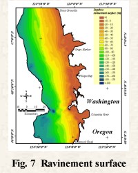
area. As with the northern part of the study area, adjustments were made to use
1,600 m/s as the speed of sound in sediment. The completed ravinement surface
is shown in Figure 7.
In order to get the sediment distribution and
thickness values of the merged data to honor the isopach map of Wolf and others
(1997), 7 m needed to be added to the negative depth values of their erosional
surface map effectively raising the surface. This adjustment enabled the merged
data set to honor Wolf´s and others´ (1997) interpreted isopach values and the
approximate sediment accumulation in the offshore area. In fact, this adjustment
had the sediment contribution offshore from their interpretation to be 38 km3
which is much closer to the values extracted directly from their interpretation. Once
the data integration was accomplished, it was fairly simple to
further modify these data points from a speed of sound of 1,640 m/s to the
1,600 m/s used in this study. Wolf´s and others´ (1997) data points were used
to extract the corresponding seafloor depths from the modern surface grid using
the Arc/Info AML "gridspot70.aml". An awk script was used to take the difference between
these seafloor depths and structure depths and recalculate a new ravinement
structure depth using 1,600 m/s for the speed of sound in sediment. These new
point values were then combined with the near- and on-shore data to generate the
ravinement surface. This technique for incorporating the outer shelf data worked
very well north of the Columbia River. Unfortunately, south of the mouth of the
Columbia River was much more complicated. In this area, Twichell used
ArcView (URL: http://www.esri.com) to select points and assign depths to the ravinement surface values
based on Wolf´s and others (1997) isopach interpretation. Although more user intensive, this
technique honored the interpretation of Wolf and others (1997) while at the same
time avoiding problems in the bathymetrically more complex portion of the study
area. As with the northern part of the study area, adjustments were made to use
1,600 m/s as the speed of sound in sediment. The completed ravinement surface
is shown in Figure 7.
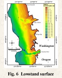 The generation of this surface also incorporated
a wide variety of data sets. In Grays Harbor and Willapa Bay existing
interpretations from Peterson and Phipps
(1992), and Wolf and others (1998)
respectively were digitized. In a manner similar to the ravinement surface
offshore data, these structure contours were densified to get a point every 100
m. In Grays Harbor, Peterson and Phipps (1992) used
a value of 1600 m/s for speed of sound. Because the water is so shallow in this area, no attempt was made to
adjust for the difference between the water column portion of the depth
measurement and the depth to the structure surface. In Willapa Bay, 1,500 m/s
was the value for the speed of sound. As with other data derived from contour maps,
the arcs were densified and a vertex every 100 m was extracted. The same "gridspot"
technique described for the ravinement surface was used to make the speed of
sound adjustment. The offshore area used Wolf´s
and others´ (1997) data
describing the ravinement surface to represent the lowstand surface as well. The
corrections to these values had already been applied during the ravinement
surface generation. The lowstand surface is shown in Figure
6.
The generation of this surface also incorporated
a wide variety of data sets. In Grays Harbor and Willapa Bay existing
interpretations from Peterson and Phipps
(1992), and Wolf and others (1998)
respectively were digitized. In a manner similar to the ravinement surface
offshore data, these structure contours were densified to get a point every 100
m. In Grays Harbor, Peterson and Phipps (1992) used
a value of 1600 m/s for speed of sound. Because the water is so shallow in this area, no attempt was made to
adjust for the difference between the water column portion of the depth
measurement and the depth to the structure surface. In Willapa Bay, 1,500 m/s
was the value for the speed of sound. As with other data derived from contour maps,
the arcs were densified and a vertex every 100 m was extracted. The same "gridspot"
technique described for the ravinement surface was used to make the speed of
sound adjustment. The offshore area used Wolf´s
and others´ (1997) data
describing the ravinement surface to represent the lowstand surface as well. The
corrections to these values had already been applied during the ravinement
surface generation. The lowstand surface is shown in Figure
6.
Because EarthVision uses a spline gridding technique, any areas with dramatic changes in elevation can be troublesome. A spline fit to data points where there are sharp changes in elevation tend to cause overshoots of the data. This might translate to be a deep trough next to a sea cliff if there were no data points available at the base of the cliff. The gridding software had trouble on all three surfaces along the Columbia River. In each case, additional points were manually added to aid the gridding software in areas of sparse data. For the Columbia River, points were added (particularly to the lowstand surface), such that the river maintained a down slope gradient. In other words, each surface was checked manually for geologic validity, and correction values applied as necessary. In this manner, the 200-m grid cell size was maintained while at the same time honoring geologic principles.
Once satisfied with the three surfaces, each grid was run through one pass of EarthVision´s low-pass filter to smooth local variations in the grid. After this filtering process was complete, one more correction was applied to the ravinement and lowstand surfaces. The gridding of the individual surfaces did not incorporate upper and lower boundary constraints, therefore it became possible for a lower surface to exceed or "stick above" an overlying surface. Due to the nature of the surfaces defined in this area, the lower surface should be below or equal to its overlying surface. In order to enforce this principle, simple grid math was done on the surfaces in EarthVision. For the ravinement surface, if the grid values were less than or equal to the present day surface (because values were negative) the ravinement grid values were used. If the ravinement grid values were greater than present day cell values at the same location, then the ravinement values were set equal to the present day values. This same correction was then applied to the lowstand surface with respect to the ravinement surface.
The collaborators on the Southwest Washington Coastal Erosion Study chose ESRI´s ArcView/ArcInfo (http://www.esri.com) as the common format with which to share GIS files, hence the need to convert the EarthVision grids to an ESRI compatible format. The Spatial Analyst and 3D Analyst extensions of ArcView are required and/or a Grid license for Arc/Info because the analyses of these data will utilize grids and tins,. The first step in the grid conversion process was to export each EarthVision grid as an ascii grid. The second step was to effectively "flip" the grid. EarthVision places the grid origin as the lower left corner of the grid while ArcView uses the upper left corner as the grid origin. Running the EarthVision ascii grid through an awk script changed the order of the rows while leaving the column values in the same order. This "flipped" ascii file was then run through another awk script which reformatted the file and added the appropriate header to comply with ESRI´s ascii grid format. This new ascii grid could then be imported into ArcView or Arc/Info without any difficulties.
EarthVision´s gridding extrapolates data values outside the study area, yet these data values needed to be converted to null values. This required that the grid be clipped to the study area polygon. This clipping process could actually occur at any point during analysis, but was our initial processing step in ArcView to avoid confusion with the grids and what values were accepted as realistic.
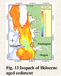
The first calculated grids, namely the isopach maps, were the easiest to derive. These isopach maps were created by subtracting the lowstand surface (Fig. 6) from the ravinement surface (Fig. 7) to generate the isopach map shown in Figure 12. Subtracting the ravinement surface (Fig. 7) from the present day surface (Fig. 8) resulted in the ispoach map shown in Figure 13. Values derived from the calculations are given in the Geologic Discussion section. Significantly more complex were the calculations necessary to derive isochron surfaces at 1,000-year intervals.

One goal of this study was to see how the coast evolved during the Holocene. In order to accomplish this goal, the task of generating surfaces every 1,000 years was undertaken. Several assumptions were necessary to simplify this process. 1) sedimentation in the bays and on the shelf did not start before 14,000 yr BP, 2) sedimentation on the shelf occurs at a constant rate since the last lowstand of sea level, 3) sediment filling of the bays keeps pace with sea level rise, and 4) intersection of the sea level curve with the ravinement surface marks the landward edge of shelf sediment deposition. Although the maximum lowstand was 15,000 yr BP in the study area, the isochron surfaces were initiated 11,000 yr BP. A greater degree of confidence is attributed to the age dates and sea levels starting at 11,000 yr BP.
The technique to calculate the surfaces can be broken into two distinct time frames. From 11,000 yr BP to 5,000 yr BP the coastline simply retreated across the shelf as sea level rose. During this time interval, the only preserved deposits were from the shelf and bays which simplified the surface calculations. Based on age information from the barriers (Herb, 2000; Woxell, 1998), beaches started prograding in the study area starting about 5,000 yr BP, although sea level continued to rise. This step required the last 5,000 years to have slightly different calculations, as well as adding beach deposits to the framework of volumes to be calculated.
In order to derive volume calculations of the various depositional environments through time, these 1,000-year surfaces are needed. However, by providing the digital data with this report, modifications and improvements to the technique are possible and encouraged. Perhaps the easiest way to describe the calculation techniques used in this study is to use examples from pre- and post- beach progradation times.
Here the 10,000 yr BP time interval will be used as the example of
pre-progradation surface development. At 10,000 yr BP, sea level was 47 m below
present day sea level (Fig. 3). The first step is to find the 47 m contour on
the ravinement surface (Fig. 7), which is a simple procedure within ArcView. The
resulting contour was simplified so that it represented a single line, which
when merged with the study area bounding polygon, generated 2 polygons (Fig.
16). 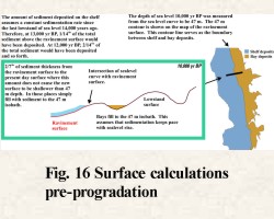 The seaward polygon delineates the area of shelf deposits, while the landward
polygon delineates the bay deposits. The calculations of the seaward polygon are
performed on the ravinement surface. Essentially, the ravinement grid is clipped
to the seaward part of the polygon. The amount of sediment deposited on the
shelf assumes a constant sedimentation rate since sediment accumulation started
14,000 years ago in the study area. Therefore, at 13,000 yr BP, 1/14th
of the total sediment above the ravinement surface would have been deposited. At
12,000 yr BP, 2/14th of the total sediment would have been deposited
and so forth. In this example, 2/7th (or 4/14ths) of the sediment
thickness from the ravinment to the present day surface is deposited. The
limitation on this approach is that deposition cannot cause the new surface to be
shallower than the 47 m isobath. In those areas where adding the total sediment
thickness would violate this limitation, the shelf is simply filled to the 47 m
isobath (see cross-section shown in Fig. 16). In the landward polygon, the calculations are performed on the lowstand
surface rather than the ravinement surface. Here, the landward polygon is used
as the clipping bounds on the lowstand grid, with subsequent calculations
performed on this clipped grid. Honoring the assumption that sediment
accumulation in the bays keeps pace with sea level rise, any values on the
lowstand surface less than 47 m are filled to 47 m (Fig. 16).
The seaward polygon delineates the area of shelf deposits, while the landward
polygon delineates the bay deposits. The calculations of the seaward polygon are
performed on the ravinement surface. Essentially, the ravinement grid is clipped
to the seaward part of the polygon. The amount of sediment deposited on the
shelf assumes a constant sedimentation rate since sediment accumulation started
14,000 years ago in the study area. Therefore, at 13,000 yr BP, 1/14th
of the total sediment above the ravinement surface would have been deposited. At
12,000 yr BP, 2/14th of the total sediment would have been deposited
and so forth. In this example, 2/7th (or 4/14ths) of the sediment
thickness from the ravinment to the present day surface is deposited. The
limitation on this approach is that deposition cannot cause the new surface to be
shallower than the 47 m isobath. In those areas where adding the total sediment
thickness would violate this limitation, the shelf is simply filled to the 47 m
isobath (see cross-section shown in Fig. 16). In the landward polygon, the calculations are performed on the lowstand
surface rather than the ravinement surface. Here, the landward polygon is used
as the clipping bounds on the lowstand grid, with subsequent calculations
performed on this clipped grid. Honoring the assumption that sediment
accumulation in the bays keeps pace with sea level rise, any values on the
lowstand surface less than 47 m are filled to 47 m (Fig. 16).
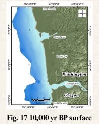 The final step in generating the 10,000 yr BP
surface is to merge these 2 grids into a single grid. To eliminate any possible
null values at the polygon boundaries, a low-pass filter was performed on the
combined grid. Because this low-pass filter also extrapolates a bit beyond the
study area boundaries, these grids are then re-clipped to the bounding polygon.
In order to have a more realistic looking surface for the time frame, this
surface is then shifted by a value equal to the depth to the sea level curve at
that time. In this example, a value of 47 was added to each grid cell value. This
shift has two benefits: 1) the zero value now represents the shoreline at that
time, and 2) the same legend can be used with all the grid surfaces. In addition
to this shift, the modern day DEM was shifted by the same amount and combined
with the 10,000 yr BP surface. One final aesthetic step was applied, and that
was to use the modern day bathymetric values of the Columbia River outside the
study area to maintain the presence of the river (Fig. 17). This technique,
using the different sea level values, is repeated for every surface prior to
beach progradation. Each 1,000-year surface derived it values based on the
original ravinement and lowstand surfaces rather than building on the previous
1,000-year surface. The reason to do this was to avoid a "stair-step"
pattern on the shelf deposits resulting from the flat deposit area immediately
adjacent to the shelf/bay boundary (Fig. 16).
The final step in generating the 10,000 yr BP
surface is to merge these 2 grids into a single grid. To eliminate any possible
null values at the polygon boundaries, a low-pass filter was performed on the
combined grid. Because this low-pass filter also extrapolates a bit beyond the
study area boundaries, these grids are then re-clipped to the bounding polygon.
In order to have a more realistic looking surface for the time frame, this
surface is then shifted by a value equal to the depth to the sea level curve at
that time. In this example, a value of 47 was added to each grid cell value. This
shift has two benefits: 1) the zero value now represents the shoreline at that
time, and 2) the same legend can be used with all the grid surfaces. In addition
to this shift, the modern day DEM was shifted by the same amount and combined
with the 10,000 yr BP surface. One final aesthetic step was applied, and that
was to use the modern day bathymetric values of the Columbia River outside the
study area to maintain the presence of the river (Fig. 17). This technique,
using the different sea level values, is repeated for every surface prior to
beach progradation. Each 1,000-year surface derived it values based on the
original ravinement and lowstand surfaces rather than building on the previous
1,000-year surface. The reason to do this was to avoid a "stair-step"
pattern on the shelf deposits resulting from the flat deposit area immediately
adjacent to the shelf/bay boundary (Fig. 16).
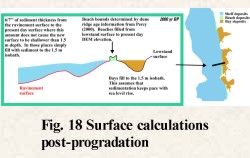 Dune
ridge ages (Woxell, 1998; Peterson and others,
1999; Herb, 2000; Reckendorf and others, 2001)
indicate that beach progradation began at least 5,000 yr BP. This information had to be incorporated
into the surface generation. For this reason, the boundary between shelf and bay
deposits can no longer be derived simply by the intersection of the sea level
curve with the ravinement surface. This isobath is used in part, but we incorporated the dune ridge information as well as interpreting
shelf/bay boundaries at the mouths of estuaries. The onset of beach progradation
now means there are three depositional environments: shelf, bay and beach (Fig.
18). For illustration purposes, the 2,000 yr BP surface is used. The shelf and bay calculations are done the same as prior to beach
progradation.
Dune
ridge ages (Woxell, 1998; Peterson and others,
1999; Herb, 2000; Reckendorf and others, 2001)
indicate that beach progradation began at least 5,000 yr BP. This information had to be incorporated
into the surface generation. For this reason, the boundary between shelf and bay
deposits can no longer be derived simply by the intersection of the sea level
curve with the ravinement surface. This isobath is used in part, but we incorporated the dune ridge information as well as interpreting
shelf/bay boundaries at the mouths of estuaries. The onset of beach progradation
now means there are three depositional environments: shelf, bay and beach (Fig.
18). For illustration purposes, the 2,000 yr BP surface is used. The shelf and bay calculations are done the same as prior to beach
progradation.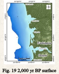 But it is more than likely that there are multiple bay polygons. Since
the boundary delineating the bay deposits is no longer based on a contour value,
the additional caveat was added that the value of the bay portion of the surface
must be less than or equal to the present day surface. The reason for this change is because
the bathymetry shows channels in each of the bays with floors deeper than the
sea level depth. Although this restriction wasn´t placed on the bay deposits
until the 5,000 yr BP surface, it could have been applied to all the 1,000-year
surfaces. For the beach deposits, the beach polygons are used to clip the
ravinement surface. Since there is no information pertaining to historic beach
elevations, these beach polygons are filled to the present day DEM (Fig.
18). In reality, this step of using the beach polygons as a clipping boundary is
unnecessary. The appropriate grid merge sequence could be used to incorporate
the present day surface with the bay and shelf polygons. As described in the
Pre-Progradation section, once the individual depositional environments
are calculated, these grids are then merged together to form the surface from
that time frame and have a low-pass filter applied to remove any possible null values at the polygon boundaries. Likewise, these filtered surfaces are clipped
with the study area polygon. They are then shifted based on the sea level curve, and
merged with the shifted present day DEM and the present day Columbia River
bathymetric values (Fig. 19).
But it is more than likely that there are multiple bay polygons. Since
the boundary delineating the bay deposits is no longer based on a contour value,
the additional caveat was added that the value of the bay portion of the surface
must be less than or equal to the present day surface. The reason for this change is because
the bathymetry shows channels in each of the bays with floors deeper than the
sea level depth. Although this restriction wasn´t placed on the bay deposits
until the 5,000 yr BP surface, it could have been applied to all the 1,000-year
surfaces. For the beach deposits, the beach polygons are used to clip the
ravinement surface. Since there is no information pertaining to historic beach
elevations, these beach polygons are filled to the present day DEM (Fig.
18). In reality, this step of using the beach polygons as a clipping boundary is
unnecessary. The appropriate grid merge sequence could be used to incorporate
the present day surface with the bay and shelf polygons. As described in the
Pre-Progradation section, once the individual depositional environments
are calculated, these grids are then merged together to form the surface from
that time frame and have a low-pass filter applied to remove any possible null values at the polygon boundaries. Likewise, these filtered surfaces are clipped
with the study area polygon. They are then shifted based on the sea level curve, and
merged with the shifted present day DEM and the present day Columbia River
bathymetric values (Fig. 19).
Once all the surfaces and isopachs are generated, volume calculations become a simple task. Within ArcView, volume calculation requires that a grid first be converted to a tin. A vertical tolerance is defined by the user during this conversion. For this study, a tolerance of 0.5 m was used. This corresponds well with our perceived vertical resolution and accuracy of the data. Once the tin of interest is created, it needs to be edited to add the bounding polygon features as a clipping feature. The newly resulting tin is then evaluated for volume. To determine the amount of sediment from each depositional environment, the 1,000-year surfaces were used. For example, the first step to calculate the amount of shelf, bay and beach sediment deposited from 3,000 yr BP to 2,000 yr BP is to subtract the 3,000 yr BP surface from the 2,000 yr BP surface. This isopach grid is then converted to a tin using the 0.5m vertical tolerance value. The resulting tin is then edited to add the polygon features used to generate the 2,000-year surface. By selecting the shelf polygon(s), only those selected features are used to clip the tin. This new tin is saved as a separate file. By selecting only the bay polygon(s) and adding those features to the original isopach tin, the tin is then clipped to the bay areas. This procedure was then be repeated for the beach polygon(s). The result is three separate tins clipped based on depositional environments. Volumes of each tin are then calculated quickly and easily with ArcView. The volumes presented in this report are calculated above a base height of zero (Fig. 14). This is based on the assumption that an earlier surface should not exceed a later surface in elevation. In areas where these restrictions were not built into the surface calculations, this method of calculating volume addresses this issue. For instance, prior to the 5,000 yr BP surface, the bay elevations were not forced to be less than or equal to the present day surface. Also, applying a low-pass filter to the surfaces after the merging of the individual grids could potentially introduce the same type of error.